
E&CE 327: Digital Systems Engineering Lab Manual Mark Aagaard 2014t2 (Spring)
E&CE 327: Digital Systems Engineering
Lab Manual
Mark Aagaard
2014t2 (Spring)
University of Waterloo
Dept of Electrical and Computer Engineering
Table of Contents
Handout 1: Environment Configuration
1
Connecting to an ECE-Linux Computer . . . . . . .
1.1
Connection from MS-Windows: MobaXterm
1.2
Connection from Linux . . . . . . . . . . . .
1.3
Connection from Mac OS . . . . . . . . . .
2
Editors and Shells . . . . . . . . . . . . . . . . . . .
3
ECE-Linux Configuration . . . . . . . . . . . . . . .
4
ECE-Linux Manual Configuration . . . . . . . . . .
4.1
Finding Your Shell . . . . . . . . . . . . . .
4.2
Bash Shell Configuration . . . . . . . . . . .
4.3
Csh and Tcsh Shell Configuration . . . . . .
5
Nexus Configuration . . . . . . . . . . . . . . . . .
.
.
.
.
.
.
.
.
.
.
.
2
2
2
2
2
3
3
3
3
4
4
5
Handout 2: Local Scripts and Project Files
1
Scripts . . . . . . . . . . . . . . . . . . . . . . . . . . . . . . . . . . . . . . . . . . . . . .
2
UW Project Files . . . . . . . . . . . . . . . . . . . . . . . . . . . . . . . . . . . . . . . .
3
Locally Added Simulation Commands . . . . . . . . . . . . . . . . . . . . . . . . . . . . .
6
6
7
9
Handout 3: Timing Simulation
1
Zero-Delay Circuit Simulation . . . . . .
2
Where Timing Simulation Comes In . . .
3
What Timing Simulation Does . . . . . .
4
Performing a Timing Simulation . . . . .
5
Debugging in Chip and Timing Simulation
5.1
Bugs in Chip Simulation . . . . .
5.2
Bugs in Timing Simulation . . . .
.
.
.
.
.
.
.
.
.
.
.
.
.
.
.
.
.
.
.
.
.
.
.
.
.
.
.
.
.
.
.
.
.
.
.
.
.
.
.
.
.
.
.
.
.
.
.
.
.
.
.
.
.
.
.
.
.
.
.
.
.
.
.
.
.
.
.
.
.
.
.
.
.
.
.
.
.
.
.
.
.
.
.
.
.
.
.
.
.
.
.
.
.
.
.
.
.
.
.
.
.
.
.
.
.
.
.
.
.
.
.
.
.
.
.
.
.
.
.
.
.
.
.
.
.
.
.
.
.
.
.
.
.
.
.
.
.
.
.
.
.
.
.
.
.
.
.
.
.
.
.
.
.
.
.
.
.
.
.
.
.
.
.
.
.
.
.
.
.
.
.
.
.
.
.
.
.
.
.
.
.
.
.
.
.
.
.
.
.
.
.
.
.
.
.
.
.
.
.
.
.
.
.
.
.
.
.
.
.
.
.
.
.
.
.
.
.
.
.
.
.
.
.
.
.
.
.
.
.
.
.
.
.
.
.
.
.
.
.
.
.
.
.
.
.
.
.
.
.
.
.
.
.
.
.
.
.
.
.
.
.
.
.
.
.
.
.
.
.
.
.
.
.
.
.
.
.
.
.
.
.
.
.
.
.
.
.
.
.
.
.
.
.
.
.
.
.
.
.
.
.
.
.
.
.
.
.
.
.
.
.
.
.
.
.
.
.
.
.
.
.
.
.
.
.
.
.
.
.
.
.
.
.
.
.
.
.
.
.
.
.
.
.
.
.
.
.
.
.
.
.
.
.
.
.
.
.
.
.
.
.
.
.
.
.
.
.
.
.
.
.
.
.
.
.
.
.
.
.
.
.
.
.
.
.
.
.
.
.
.
.
.
.
.
.
.
.
.
.
.
.
.
.
.
.
.
.
.
.
10
10
10
10
11
11
11
12
Handout 5: Warning and Error Messages
13
1
Warning Messages from PrecisionRTL (uw-synth) . . . . . . . . . . . . . . . . . . . . . . . 13
2
Error Message . . . . . . . . . . . . . . . . . . . . . . . . . . . . . . . . . . . . . . . . . . 14
Handout 4: Debugging Latches and Combinational Loops
15
1
Finding Latches . . . . . . . . . . . . . . . . . . . . . . . . . . . . . . . . . . . . . . . . . 15
2
Finding Combinational Loops . . . . . . . . . . . . . . . . . . . . . . . . . . . . . . . . . 15
Lab 1: Adders and Flip-Flops
17
1
Overview . . . . . . . . . . . . . . . . . . . . . . . . . . . . . . . . . . . . . . . . . . . . 17
2
Lab Setup . . . . . . . . . . . . . . . . . . . . . . . . . . . . . . . . . . . . . . . . . . . . 17
1
ECE-327: 2014t2 (Spring)
3
4
5
Lab 2:
1
2
3
4
5
Adders . . . . . . . . . . . . . . . . . . .
3.1
Sum . . . . . . . . . . . . . . . .
3.2
Carry . . . . . . . . . . . . . . .
3.3
One-bit Full Addder . . . . . . .
3.4
Two-bit Addder . . . . . . . . . .
Flip Flops . . . . . . . . . . . . . . . . .
4.1
Flip-flop with Synchronous Reset
4.2
Flip-flop with Chip Enable . . . .
4.3
Flip-flop with Mux on Input . . .
4.4
Flip-flop with Feedback . . . . .
Lab Submission . . . . . . . . . . . . . .
TABLE OF CONTENTS
.
.
.
.
.
.
.
.
.
.
.
.
.
.
.
.
.
.
.
.
.
.
.
.
.
.
.
.
.
.
.
.
.
.
.
.
.
.
.
.
.
.
.
.
.
.
.
.
.
.
.
.
.
.
.
.
.
.
.
.
.
.
.
.
.
.
.
.
.
.
.
.
.
.
.
.
.
.
.
.
.
.
.
.
.
.
.
.
.
.
.
.
.
.
.
.
.
.
.
Statemachines and Datapaths
Overview . . . . . . . . . . . . . . . . . . . . . . . . . .
Lab Setup . . . . . . . . . . . . . . . . . . . . . . . . . .
Heating System . . . . . . . . . . . . . . . . . . . . . . .
3.1
Heating System Implementation . . . . . . . . . .
3.2
Heating System Testbench . . . . . . . . . . . . .
Low-Pass Filter . . . . . . . . . . . . . . . . . . . . . . .
4.1
Basic Mathematics . . . . . . . . . . . . . . . . .
4.2
System Architecture . . . . . . . . . . . . . . . .
4.3
Basic Connectivity Test for Audio . . . . . . . . .
4.4
Thin-Line Implementation . . . . . . . . . . . . .
4.5
Audacity Software for Waveform Analysis . . . .
4.6
Testbench . . . . . . . . . . . . . . . . . . . . . .
4.7
Synthesis . . . . . . . . . . . . . . . . . . . . . .
4.8
Averaging Filter with Selectable Source and Output
4.9
Low-Pass Filter . . . . . . . . . . . . . . . . . . .
Lab Submission . . . . . . . . . . . . . . . . . . . . . . .
Lab3: Preview of the Project
1
Overview . . . . . . . . . . . . . . . . . . . . . . . .
2
Algorithm . . . . . . . . . . . . . . . . . . . . . . . .
3
System Architecture and Provided Code . . . . . . . .
4
Lab Setup . . . . . . . . . . . . . . . . . . . . . . . .
5
System Requirements . . . . . . . . . . . . . . . . . .
5.1
Coding Requirements . . . . . . . . . . . . .
5.2
System Initialization . . . . . . . . . . . . . .
5.3
Reset . . . . . . . . . . . . . . . . . . . . . .
5.4
Behaviour . . . . . . . . . . . . . . . . . . . .
5.5
Data and Clock Synchronization . . . . . . . .
5.6
Memory . . . . . . . . . . . . . . . . . . . . .
6
Procedure and Deliverables . . . . . . . . . . . . . . .
6.1
Design Hints . . . . . . . . . . . . . . . . . .
7
Design Procedure . . . . . . . . . . . . . . . . . . . .
7.1
Functional Simulation . . . . . . . . . . . . .
7.2
Download to FPGA and Running on the FPGA
8
Lab Submission . . . . . . . . . . . . . . . . . . . . .
.
.
.
.
.
.
.
.
.
.
.
.
.
.
.
.
.
.
.
.
.
.
.
.
.
.
.
.
.
.
.
.
.
.
.
.
.
.
.
.
.
.
.
.
.
.
.
.
.
.
.
.
.
.
.
.
.
.
.
.
.
.
.
.
.
.
.
.
.
.
.
.
.
.
.
.
.
.
.
.
.
.
.
.
.
.
.
.
.
.
.
.
.
.
.
.
.
.
.
.
.
.
.
.
.
.
.
.
.
.
.
.
.
.
.
.
.
.
.
.
.
.
.
.
.
.
.
.
.
.
.
.
.
.
.
.
.
.
.
.
.
.
.
.
.
.
.
.
.
.
.
.
.
.
.
.
.
.
.
.
.
.
.
.
.
.
.
.
.
.
.
.
.
.
.
.
.
.
.
.
.
.
.
.
.
.
.
.
.
.
.
.
.
.
.
.
.
.
.
.
.
.
.
.
.
.
.
.
.
.
.
.
.
.
.
.
.
.
.
.
.
.
.
.
.
.
.
.
.
.
.
.
17
17
18
18
19
20
20
21
21
22
22
.
.
.
.
.
.
.
.
.
.
.
.
.
.
.
.
.
.
.
.
.
.
.
.
.
.
.
.
.
.
.
.
.
.
.
.
.
.
.
.
.
.
.
.
.
.
.
.
.
.
.
.
.
.
.
.
.
.
.
.
.
.
.
.
.
.
.
.
.
.
.
.
.
.
.
.
.
.
.
.
.
.
.
.
.
.
.
.
.
.
.
.
.
.
.
.
.
.
.
.
.
.
.
.
.
.
.
.
.
.
.
.
.
.
.
.
.
.
.
.
.
.
.
.
.
.
.
.
.
.
.
.
.
.
.
.
.
.
.
.
.
.
.
.
.
.
.
.
.
.
.
.
.
.
.
.
.
.
.
.
.
.
.
.
.
.
.
.
.
.
.
.
.
.
.
.
.
.
.
.
.
.
.
.
.
.
.
.
.
.
.
.
.
.
.
.
.
.
.
.
.
.
.
.
.
.
.
.
.
.
.
.
.
.
.
.
.
.
.
.
.
.
.
.
.
.
.
.
.
.
.
.
.
.
.
.
.
.
.
.
.
.
.
.
.
.
.
.
.
.
.
.
.
.
.
.
.
.
.
.
.
.
.
.
.
.
.
.
.
.
.
.
.
.
.
.
.
.
.
.
.
.
.
.
.
.
.
.
23
23
23
23
23
24
25
25
25
26
27
28
28
29
29
30
31
.
.
.
.
.
.
.
.
.
.
.
.
.
.
.
.
.
.
.
.
.
.
.
.
.
.
.
.
.
.
.
.
.
.
.
.
.
.
.
.
.
.
.
.
.
.
.
.
.
.
.
.
.
.
.
.
.
.
.
.
.
.
.
.
.
.
.
.
.
.
.
.
.
.
.
.
.
.
.
.
.
.
.
.
.
.
.
.
.
.
.
.
.
.
.
.
.
.
.
.
.
.
.
.
.
.
.
.
.
.
.
.
.
.
.
.
.
.
.
.
.
.
.
.
.
.
.
.
.
.
.
.
.
.
.
.
.
.
.
.
.
.
.
.
.
.
.
.
.
.
.
.
.
.
.
.
.
.
.
.
.
.
.
.
.
.
.
.
.
.
.
.
.
.
.
.
.
.
.
.
.
.
.
.
.
.
.
.
.
.
.
.
.
.
.
.
.
.
.
.
.
.
.
.
.
.
.
.
.
.
.
.
.
.
.
.
.
.
.
.
.
.
.
.
.
.
.
.
.
.
.
.
.
.
.
.
.
.
.
.
.
.
.
.
.
.
.
.
.
.
.
.
.
.
.
.
.
.
.
.
.
.
.
.
.
.
.
.
.
.
.
.
.
.
.
.
.
.
.
.
.
.
.
.
.
.
.
.
.
.
.
.
.
.
.
.
.
.
.
.
.
.
.
.
.
.
32
32
32
33
36
36
36
37
37
37
38
38
38
38
39
42
42
43
2
ECE-327: 2014t2 (Spring)
Project: Kirsch Edge Detecter
1
Overview . . . . . . . . . . . . . . . . . . . . .
1.1
Edge Detection . . . . . . . . . . . . . .
1.2
System Implementation . . . . . . . . .
1.3
Running the Edge Detector . . . . . . . .
1.4
Provided Code . . . . . . . . . . . . . .
2
Requirements . . . . . . . . . . . . . . . . . . .
2.1
System Modes . . . . . . . . . . . . . .
2.2
System Initialization . . . . . . . . . . .
2.3
Input/Output Protocol . . . . . . . . . .
2.4
Row Count of Incoming Pixels . . . . . .
2.5
Memory . . . . . . . . . . . . . . . . . .
3
Design and Optimization Procedure . . . . . . .
3.1
Reference Model Specification . . . . . .
3.2
Equations and Pseudocode . . . . . . . .
3.3
Dataflow Diagram . . . . . . . . . . . .
3.4
Implementation . . . . . . . . . . . . . .
3.5
Functional Simulation . . . . . . . . . .
3.6
High-level Optimizations . . . . . . . . .
3.7
Timing Simulation . . . . . . . . . . . .
3.8
Peephole Optimizations . . . . . . . . .
3.9
Implement on FPGA . . . . . . . . . . .
4
Deliverables . . . . . . . . . . . . . . . . . . . .
4.1
Group Registration . . . . . . . . . . . .
4.2
Dataflow Diagram . . . . . . . . . . . .
4.3
Project . . . . . . . . . . . . . . . . . .
4.4
Design Report . . . . . . . . . . . . . .
4.5
Demo . . . . . . . . . . . . . . . . . . .
5
Marking . . . . . . . . . . . . . . . . . . . . . .
5.1
Functional Testing . . . . . . . . . . . .
5.2
Optimality Testing . . . . . . . . . . . .
5.3
Performance and Optimality Calculation .
5.4
Marking Scheme . . . . . . . . . . . . .
5.5
Late Penalties . . . . . . . . . . . . . . .
A
Statistics for Optimality Measurements . . . . . .
3
TABLE OF CONTENTS
.
.
.
.
.
.
.
.
.
.
.
.
.
.
.
.
.
.
.
.
.
.
.
.
.
.
.
.
.
.
.
.
.
.
.
.
.
.
.
.
.
.
.
.
.
.
.
.
.
.
.
.
.
.
.
.
.
.
.
.
.
.
.
.
.
.
.
.
.
.
.
.
.
.
.
.
.
.
.
.
.
.
.
.
.
.
.
.
.
.
.
.
.
.
.
.
.
.
.
.
.
.
.
.
.
.
.
.
.
.
.
.
.
.
.
.
.
.
.
.
.
.
.
.
.
.
.
.
.
.
.
.
.
.
.
.
.
.
.
.
.
.
.
.
.
.
.
.
.
.
.
.
.
.
.
.
.
.
.
.
.
.
.
.
.
.
.
.
.
.
.
.
.
.
.
.
.
.
.
.
.
.
.
.
.
.
.
.
.
.
.
.
.
.
.
.
.
.
.
.
.
.
.
.
.
.
.
.
.
.
.
.
.
.
.
.
.
.
.
.
.
.
.
.
.
.
.
.
.
.
.
.
.
.
.
.
.
.
.
.
.
.
.
.
.
.
.
.
.
.
.
.
.
.
.
.
.
.
.
.
.
.
.
.
.
.
.
.
.
.
.
.
.
.
.
.
.
.
.
.
.
.
.
.
.
.
.
.
.
.
.
.
.
.
.
.
.
.
.
.
.
.
.
.
.
.
.
.
.
.
.
.
.
.
.
.
.
.
.
.
.
.
.
.
.
.
.
.
.
.
.
.
.
.
.
.
.
.
.
.
.
.
.
.
.
.
.
.
.
.
.
.
.
.
.
.
.
.
.
.
.
.
.
.
.
.
.
.
.
.
.
.
.
.
.
.
.
.
.
.
.
.
.
.
.
.
.
.
.
.
.
.
.
.
.
.
.
.
.
.
.
.
.
.
.
.
.
.
.
.
.
.
.
.
.
.
.
.
.
.
.
.
.
.
.
.
.
.
.
.
.
.
.
.
.
.
.
.
.
.
.
.
.
.
.
.
.
.
.
.
.
.
.
.
.
.
.
.
.
.
.
.
.
.
.
.
.
.
.
.
.
.
.
.
.
.
.
.
.
.
.
.
.
.
.
.
.
.
.
.
.
.
.
.
.
.
.
.
.
.
.
.
.
.
.
.
.
.
.
.
.
.
.
.
.
.
.
.
.
.
.
.
.
.
.
.
.
.
.
.
.
.
.
.
.
.
.
.
.
.
.
.
.
.
.
.
.
.
.
.
.
.
.
.
.
.
.
.
.
.
.
.
.
.
.
.
.
.
.
.
.
.
.
.
.
.
.
.
.
.
.
.
.
.
.
.
.
.
.
.
.
.
.
.
.
.
.
.
.
.
.
.
.
.
.
.
.
.
.
.
.
.
.
.
.
.
.
.
.
.
.
.
.
.
.
.
.
.
.
.
.
.
.
.
.
.
.
.
.
.
.
.
.
.
.
.
.
.
.
.
.
.
.
.
.
.
.
.
.
.
.
.
.
.
.
.
.
.
.
.
.
.
.
.
.
.
.
.
.
.
.
.
.
.
.
.
.
.
.
.
.
.
.
.
.
.
.
.
.
.
.
.
.
.
.
.
.
.
.
.
.
.
.
.
.
.
.
.
.
.
.
.
.
.
.
.
.
.
.
.
.
.
.
.
.
.
.
.
.
.
.
.
.
.
.
.
.
.
.
.
.
.
.
.
.
.
.
.
.
.
.
.
.
.
.
.
.
.
.
.
.
.
.
.
.
.
.
.
.
.
.
.
44
44
45
48
48
51
51
51
52
52
53
53
54
55
55
55
57
57
58
59
59
59
60
60
60
61
61
62
62
62
63
63
64
64
65
ECE-327
Digital Systems Engineering
2014t2 (Spring)
Handout 1: Environment Configuration
The CAD tools for ece327 can be run on either the ECE Linux computers or the ECE Nexus computers.
Section 3 describes how to setup your Linux account to run the tools. Section ?? is for Nexus.
The CAD tools for ece327 run on the ECE-Linux computers.
1
Connecting to an ECE-Linux Computer
To access the ECE-Linux computers, we need to login from another computer and create an X-windows
connection. You may login from any computer (ECE Nexus, other Nexus, home, etc). We describe three
options:
Section 1.1
Section 1.2
Section 1.3
MobaXterm From Nexus
From Linux off campus
From Mac OS
The options are:
MobaXterm
ssh
Windows
Linux, Mac
simple to install and use, potentially slow
simple, potentially slow
For Mac OS X, the Linux off-campus instructions are a good starting point. If you are on an on-campus
computer with X-windows, then just ssh -X to ecelinux.
1.1
Connection from MS-Windows: MobaXterm
On Nexus, MobaXterm is at: Q:\eng\ece\util\mobaxterm.exe.
On your personal computer, you can install it from: http://mobaxterm.mobatek.net
To connext to an X-windows server, just:
1. run mobaxterm.exe
2. ssh -X ecelinux.uwaterloo.ca
1.2
Connection from Linux
For text-based interaction, you can just ssh into an ecelinux computer. For a graphical connection, use ssh
-X.
1.3
Connection from Mac OS
Mac OS (Mountain Lion (and future ones?) require ”XQuartz” in order to run X11 applications. Once
XQuarts is installed, you can just ”ssh -X ecelinux.uwaterloo.ca”.
4
ECE-327: 2014t2 (Spring)
2
Handout 1
Editors and Shells
There are several editors available on either Linux or Nexus:
Linux
Nexus
• nedit (a very simple editor)
• emacs
• pico
• gvim
• emacs
• notepad++
• vi, vim, gvim
• notepad2
• xedit
Emacs, vim, and gvim are the most powerful, and most complicated. Both emacs and vim/gvim have
VHDL modes with syntax highlighting. For the lazy, emacs even has autocompletion for VHDL. On Nexus,
notepad++ has a nice VHDL mode.
On Linux, if you are unfamiliar with emacs and vim, try starting with nedit for a simple, intuitive editor.
3
ECE-Linux Configuration
The simplest method to configure your ECE-Linux account is to run the ece327 beginning-of-term script:
/home/ece327/bin/ece327-bot
This will save a copy of your startup file (.profile for Bash and .cshrc for csh/tcsh), then create a
one-line startup file that sources the ece327 setup script.
To reverse the effects of the beginning-of-term script, run: /home/ece327/bin/ece327-bot-undo
1. You must now logout and then login again for the changes to take effect.
2. If you are happy with the results of running the beginning-of-term script, then
you may proceed directly to Lab 1 and skip the rest of this handout.
3. The remainder of this handout describes the optional manual configuration
process,
4
4.1
ECE-Linux Manual Configuration
Finding Your Shell
After you have logged into an ECE-Linux computer, and before you can configure your environment, you
need to find out which shell you are using. As your shell, you will be using csh, tcsh, or bash. To find out
which shell you are using, type:
% echo $SHELL
If the output of the above command ends in bash, then follow the instructions in Section 4.2. Otherwise,
the output should end in csh or tcsh and you should follow the instructions in Section 4.3.
If you wish to change your shell, go to:
https://eceweb.uwaterloo.ca/password
5
ECE-327: 2014t2 (Spring)
4.2
Handout 1
Bash Shell Configuration
1. If the following line is not already in your .profile file, then add the line to the end of the file:
source /home/ece327/setup-ece327.sh
2. Leave your existing session connected, and start a new connection to ECE-Linux. You need to start a
new connection to see the changes that you have made to your configuration.
3. Test the configuration:
% which precision
/opt/Precision_Synthesis_2008a.47/Mgc_home/bin/precision
% which quartus sh
/opt/altera9.0/quartus/bin/quartus sh
% which uw-clean
/home/ece327/bin/uw-clean
4. If the above commands do not work, try putting source /home/ece327/setup-ece327.sh
as the first line in your .profile file.
5. If you are unable to get your environment working correctly, then make a backup copy of your
.profile and .bashrc files and install fresh ones as shown below:
%
%
%
%
mv
cp
mv
ln
.bashrc bashrc.orig
/home/ece327/setup/bashrc .bashrc
.profile profile.orig
-s .bashrc .profile
The above commands make a copy of .bashrc and then a symbolic link from .bashrc to .profile.
If the fresh versions of these files work, then gradually add the code from your profile.orig and
bashrc.orig files back into .profile
4.3
Csh and Tcsh Shell Configuration
1. If the following line is not already in your .cshrc file, then add the line to the end of the file:
source /home/ece327/setup-ece327.csh
2. Leave your existing session connected, and start a new connection to ECE-Linux. You need to start a
new connection to see the changes that you have made to your configuration.
3. Test the configuration:
% which precision
/opt/Precision_Synthesis_2008a.47/Mgc_home/bin/precision
% which quartus sh
/opt/altera9.0/quartus/bin/quartus sh
% which uw-clean
/home/ece327/bin/uw-clean
4. If the above commands do not work, try putting source /home/ece327/setup-ece327.csh
as the first line in your .cshrc file.
6
ECE-327: 2014t2 (Spring)
Handout 1
5. If you are unable to get your environment working correctly, then make a backup copy of your
.cshrc and .login files and install fresh ones as shown below:
%
%
%
%
mv
cp
mv
cp
.login login.orig
/home/ece327/setup/login .login
.cshrc cshrc.orig
/home/ece327/setup/cshrc .cshrc
If the fresh versions of these files work, then gradually add the code from your login.orig and
cshrc.orig files back into the fresh version.
5
Nexus Configuration
Follow these steps if you wish to run the ECE-327 tools directly on a Nexus computer.
1. Login to your Nexus account
2. Map the network location \\eceserv\your userid to P:. This will allow you to switch easily
between Nexus and Linux, because the P: volume on Nexus will be the same as your home directory
on the ECE-Linux computers.
3. Choose your favourite editor
Some of the available editors are:
• emacs
• gvim
• notepad++
• notepad2
Emacs and gvim are the most powerful, and most complicated. Both emacs and gvim have VHDL
modes with syntax highlighting. For the lazy, emacs even has autocompletion for VHDL. If you are
unfamiliar with emacs and vim, notepad++ has a nice VHDL mode.
4. Environment Setup
In each DOS window in which you will run the ece327 CAD tools, you need to run 327setup:
Q:\eng\ece\util\327setup
The full name of the 327setup script is: Q:\eng\ece\util\327setup.bat.
7
ECE-327
Digital Systems Engineering
2014t2 (Spring)
Handout 2: Local Scripts and Project Files
1
Scripts
To simplify the use of the tools used in the course, a variety of scripts have been written. All of the scripts
are installed in /home/ece327/bin on ECE Linux and Y:\bin on Nexus . If you have completed the
configuration steps described in Handout 1, you should be able to run the scripts.
To run a script on
ECE Linux just type the name of the script: uw-script args
Nexus python Y:\bin\uw-script args
The scripts are:
uw-clean
uw-com
uw-sim
uw-synth
uw-dnld
uw-report
uw-add-pwr
uw-loop
Deletes all intermediate files and directories generated by the tools.
Performs syntax and type checking.
Simulation
Synthesis
Download a .sof file to the FPGA board
Print out summary of area, speed, and power
Add vcd log commands to a simulation script
Execute synthesis; timing simulation; power analysis
The main argument to uw-com, uw-sim, and uw-synth is the name of the file to compile, simulate, or
synthesize. The file may be either a VHDL file or a UW Project file, which has a .uwp extension.
The scripts create several directoris for temporary files:
LOG Log files
RPT
Area, timing, and power report files
uw tmp
work-*
Scripts and some generated temporary files
Intermediate compiled or object versions of files
Synthesis flows:
FPGA synthesis Logic synthesis is done with Mentor Graphics PrecisionRTL. Physical synthesis (place
and route) is done with Altera Quartus. PrecisionRTL writes a file uw tmp/name.edf that contains
the post-logic-synthesis design and a file uw tmp/name.tcl with TCL commands for Quartus.
ASIC synthesis Logic synthesis is done with Synopsys Design Compiler. Physical synthesis is done with
Synopsys IC Compiler.
Each simulation or synthesis script generate a Python and a TCL file in the uw tmp directory that contains
the actual commands that are run.
8
ECE-327: 2014t2 (Spring)
Handout 2
For simulation and synthesis, there are a variety of options that can be included.
Option
-h
--gui
--nogui
--i
--generics= var=value,var=value,...
or -G var=value,var=value,...
-p or --prog
-g or --gates
-l or --logic
-c or --chip
-t or --timing
-o
--sim script=SIM SCRIPT
2
Sim
√
√
√
√
Synth
√
√
√
√
√
√
√
√
√
√
√
√
√
√
Description
show a help message
start the GUI
do not start the GUI
Interactive: at end of running the script,
enable interactive execution of commands
(not available for FPGA synthesis)
assign a value to a generic parameter
simulate the VHDL program
synthesize to generic gates
logic synthesis to FPGA gates for the
Cyclone-II chip on the DE2 board, which
will be used for functional simulation and
demos.
logic+physical synthesis (place and route)
to FPGA gates for the Cyclone-II chip chip
on the DE2 board, which will be used for
timing simulation and demos.
simulate chip without timing info
simulate chip without timing info
simulate chip with timing info
synthesize for optimality measurement
simulation script (overrides SIM SCRIPT
in project file)
UW Project Files
A UW project file must end with a .uwp extension.
Entire lines may be commented out with #. Partially commented-out lines are not supported.
Each line of the file is of the form:
variable = value or variable = value1 value2 ...
All of the values for a variable must appear on a single line.
The tags for source files are named ∗ VHDL, but they accept both VHDL and Verilog files.
The variables are:
9
ECE-327: 2014t2 (Spring)
LIB VHDL
DESIGN ENTITY
DESIGN ARCH
DESIGN VHDL
TB ENTITY
TB ARCH
TB VHDL
BOARD
SIM SCRIPT
PIN FILE
Handout 2
Files that are needed for both synthesis and simulation.
Name of the top-level design entity
Archicture of the top-level design entity
Space-delimited list of VHDL files containing the design.
Name of the testbench entity
Archicture of the testbench
Space-delimited list of VHDL files containing the testbench.
FPGA board for implementation. Currently supported values are DE2 (default) and EXCAL (Altera Excalibur board).
Simulation script to run
File containing mapping of top-level design entity signals to pins on the
FPGA chip.
10
ECE-327: 2014t2 (Spring)
Handout 2
Example UWP file:
TB ENTITY
TB ARCH
TB VHDL
SIM SCRIPT
=
=
=
=
kirsch_tb
main
kirsch synth pkg.vhd string pkg.vhd kirsch unsynth pkg.vhd kirsch tb.vhd
kirsch tb.sim
DESIGN ENTITY
DESIGN ARCH
DESIGN VHDL
= kirsch
= main
= kirsch synth_pkg.vhd my units.vhd kirsch.vhd
BOARD
= DE2
# comment out old: BOARD = EXCAL
Many intermediate files are generated during the synthesis process.
∗gate∗
∗logic∗
∗chip∗
∗.sdf
∗.vcd
3
Locally Added Simulation Commands
rerun
reload
rr
11
generated from logic synthesis to generic gates
generated from logic synthesis to FPGA or ASIC cells
generated from physical (chip) synthesis
Back-annotated delay information
Value-change-dump file for power analysis
rerun the current simulation
reload (recompile) the source files
reload the source files and rerun the simulation
ECE-327
Digital Systems Engineering
2014t2 (Spring)
Handout 3: Timing Simulation
1
Zero-Delay Circuit Simulation
The simulations you have been doing up until now are zero-delay in the sense that signals moving from one
hardware component to another always arrived at their destinations at the same time. This simplification
allows the computer to simulate your design quickly.
In zero-delay simulation, all signal paths are exactly the same length. You can imagine that signals are able
to travel as fast or slow as necessary to reach their intended destinations at the exact same time. Regardless of
how you interpret it, your design is implementation independent. While it can be simulated, the simulation
does not take into account any of the particular characteristics of either the target implementation technology
or your design in terms of placement and routing. However, this kind of simulation is what you should use
for testing the logical correctness of your design. After all, there is no point in worrying about whether your
design can be synthesized, if it does not work correctly in the first place. However, while you are working on
achieving functional correctness, one should still observe proper VHDL coding practices to avoid constructs
that cannot be synthesized into FPGA-centric hardware.
2
Where Timing Simulation Comes In
Once the point has been reached that your design is functionally correct, the next step in simulation fidelity is
to accurately model the actual timing characteristics of the implementation technology you intend to use. For
the purposes of this course, the technology will be an FPGA, but it need not be when you work in a specific
industry. FPGA implementations of your design will have a very different layout and logical architecture
than, say, custom VLSI, and will therefore have different timing characteristics as well. This will imply
different performance limits because of the timing constraints that each implementation will allow, as well
as the intelligence of the routing tools that place and route the signals and/or design elements. Its up to you
as a good designer to make the judgement calls that balance cost and performance. Timing analysis is part
of what this is all about.
3
What Timing Simulation Does
Timing simulation uses the layout and routing delay information (from a placed and routed design) to give
a more accurate assessment of the behaviour of the circuit under worst-case conditions. The design which
is loaded into the simulator for timing simulation contains worst-case routing delays based on the actual
placed and routed design. For this reason, timing simulation is performed after the design has been placed
and routed. Timing simulation is more time consuming than the idealized ones, especially for currentgeneration microprocessors consisting of millions of transistors. For example, 1 microsecond of real-time
operation, can take as much as 15 minutes of simulation time! But this is what it takes to ensure that no
glitches occur in the design and that all signals reach their destination on time.
12
ECE-327: 2014t2 (Spring)
4
Handout 3
Performing a Timing Simulation
In ECE-327, there are two steps to running a timing simulation: creating the files containing the timing
information and execution of the simulation.
Use uw-synth --chip to synthesize your design all the way through place-and-route and timing analysis.
Use uw-sim --timing to do timing simulation.
5
Debugging in Chip and Timing Simulation
If your design works in zero-delay simulation and you have followed the ece327 coding guidelines, then
your design should work in timing simulation.
Debugging in chip and timing simulation is difficult, because the synthesis tools will have mapped all of your
combinational logic signals to gates and will use automatically generated names for the resulting signals.
Your registered signals will still be there with (almost) their original name, but arrays will be broken down
into individual bits.
First, identify whether your design works for each the following:
• uw-sim –prog
• uw-sim –chip
• uw-sim –timing
• on the FPGA board
Identify the first of the above situations where your design does not work correctly (e.g. works in uw-sim
–chip but fails with –timing).
If your design works with uw-sim –prog but fails uw-sim –chip
1. check for warnings in log file
2. ensure that your code follows the coding guidelines
5.1
Bugs in Chip Simulation
Chip simulation is zero-delay simulation of the synthesized design. It uses the chip.vho file for the
design.
There are two common failure modes in uw-sim –chip:
• Xs on signals: common causes are:
• latches
• multiple drivers of a signal
• combinational loops
• forgot to reset an important flop
• no Xs, but different behaviour than in uw-sim –prog. common causes are:
– incorrect interface to outside world (e.g. reading inputs in the wrong clock cycle, assuming that input
values are stable for multiple clock cycles, modified testbench from original version.)
– Beware of boolean conditions: the expression a = ’0’ evaluates to false if a is X. Thus, a value of X can
be silently converted into a normal value of 0 or 1.
13
ECE-327: 2014t2 (Spring)
5.2
Handout 3
Bugs in Timing Simulation
If your design works with uw-sim –chip but fails uw-sim –time, the problem is probably that the clock is
too fast (i.e. circuit is too slow). Try increasing the clock period in the test bench.
To debug with uw-sim –chip or uw-sim –time when Xs appear:
1. Pick a flop that should be reset and eventually gets Xs. Simulate and confirm that the flop is reset
correctly (maybe testbench is not setting reset).
2. Trace backwards through the fanin of the flop to find the flop/input that causes X
To debug with –chip or –time when there aren’t Xs, but you have different behaviour with –prog than with
–chip or –time:
1. Trace flops in the buggy simulation compare with flops in uw-sim –prog.
2. Identify first clock cycle with different behaviours in the two simulations.
3. If you need to look at comb signals in –chip or –time, there’s a difficulty because comb signals
disappeared during synth. A solution is to add debug signals to the entity for the design under test.
Example:
• In the entity:
dbg a, dbg b, dbg c : std logic;
dbg vec w, dbg vec x, dbg vec y : std logic vector(7 downto 0);
• In the architecture
dbg a <= comb signal that you want to probe
dbg b <= ...
• When the design works, comment out the debug signals in the entity and architecture
14
ECE-327
Digital Systems Engineering
2014t2 (Spring)
Handout 5: Warning and Error Messages
1
Warning Messages from PrecisionRTL (uw-synth)
• Warning, signal is not always assigned.
Storage may be needed.
This is bad: signal will be turned into a latch. Check to make sure that you are covering all possible
cases in your assignmemts, and use a fall-through “others” or “else”.
• Warning, signal should be declared on the sensitivity list of the process
If this is in a combinational process, then this is bad, because you will get a latch rather than combinational circuitry. If this is in a clocked process, then it is safe to ignore the warning.
• Warning, Multiple drivers on signal; also line line
This is bad. The probable cause is that more than one process is writing to signal.
Here’s a sample situation with multiple drivers, and an explanation of how to fix the problem:
do_red:
process (state) begin
if ( state = RED ) then
next_state <= ....
end if;
end process;
do_green:
process (state) begin
if ( state = GREEN ) then
next_state <= ....
end if;
end process;
The goal here was to organize the design so that each process handles one situation, analogous to
procedures in software. However, both do red and do green assign values to next state. For
hardware, decompose your design into processes based upon the signals that are assigned to, not based
on different situations.
For example, with a traffic light system, have one process for the north-south light and one for the
east-west light, rather than having one process for when north-south is green and another process for
when east-west is green.
The correct way to think about the organization of your code is for each process to be responsible for
a signal, or a set of closely related signals. This would then give:
15
ECE-327: 2014t2 (Spring)
Handout 5
process (state) begin
if ( state = GREEN ) then
next_state <= ...
elseif ( state = GREEN ) then
next_state <= ...
else ... [ other cases ] ...
end if;
end process;
2
Error Message
• Component comp has no visible entity binding.
In your VHDL file, you have a component named comp, but you have not compiled an entity to put in
for the component.
16
ECE-327
Digital Systems Engineering
2014t2 (Spring)
Handout 4: Debugging Latches and Combinational Loops
When doing synthesis, if you get the error message: “Design contains one or more combinational loops or
latches.”, first, look for any latches (Section 1). If you do not find any latches in your design, then look for
combinational loops (Section 2).
1
Finding Latches
1. Run uw-synth with the GUI and synthesize for generic gates (not an FPGA): uw-synth --gui
filename.
2. Open up the RTL schematic
3. On the left-side of the RTL schematic, expand Instances and look for any latches (the name will
probably begin with “lat ” or you will see “LAT” after the name).
4. Click on any latch instances and the schematic window will zoom in on the latch.
5. The output signal from the latch will probably be an automatically generated name, so you will have
to navigate around to figure out which signal in your VHDL corresponds to the latch output.
2
Finding Combinational Loops
A combinational loop can span multiple processes, and the combinational dependencies include conditionals, not just the signals on the right-hand-side of an assignment. For example, the following is a combinational loop through a and d:
process (a,b,c) begin
if a = ’0’ then
d <= b;
else
d <= c;
end if;
end process;
process (d) begin
a <= d;
end process;
There are several ways to find a combinational loop:
1. Turn combinational assignments into registed assignments until you find an assignment that, when
combinational, results in a combinational loop and, when registered, removes the combinational loop.
17
ECE-327: 2014t2 (Spring)
Handout 4
2. Use a divide-and-conquer approach by deleting large chunks of code and trying to find a minimal
subset of your program that contains the combinational loop.
3. Use the schematic browser in PrecisionRTL to visually hunt for the combinational loop. To do this,
bring up the RTL schematic and:
(a)
(b)
(c)
(d)
Right click on the signal you want to include in the trace.
Select add to trace.
On the left-side of the screen, choose Schematics → View RTL Trace.
In the RTL Trace window, right click on a signal that you are interested in and choose Trace
Backward for the number of levels you are interested in. One level at a time is usually best,
because it prevents crowding your screen with irrelevant signals and gates.
18
ECE-327
Digital Systems Engineering
2014t2 (Spring)
Lab 1: Adders and Flip-Flops
1
Overview
This lab is divided into two main problems. In Section 3 you will construct several circuits to a simple adder.
In Section 4 you will construct a variety of flip-flops.
Req 1.1:
2
Students shall work alone or in groups of two.
Lab Setup
Action:
Read Handout-1: Environment Configuration (page 2)
Action:
Read Handout-2: Local Scripts (page 6)
Action:
Copy the provided files to your local account. The commands below show how this can be
done on an ECE-Linux computer if the desired target directory is
/home/your userid/ece327/lab1. In the commands, the symbol “%” means the
Linux prompt.
% cd ˜/ece327
% cp -r /home/ece327/lab/lab1 lab1
Action:
Check that you have all of the files listed below:
add2 tb.sim
add2 tb.vhd
add2.uwp
Code 1:
3
add2.vhd
carry.vhd
fulladder.uwp
fulladder.vhd
myflipflop.vhd
sum tb.sim
sum tb.vhd
sum.uwp
sum.vhd
Register your group on Coursebook.
Adders
3.1
Sum
Code 2:
Complete the VHDL code in sum.vhd to implement the behaviour of the following Boolean
expression: sum = a xor b xor cin.
Action:
Use the command below at the operating system command prompt to check for syntax and
typechecking errors. Fix any errors in the source code until the code synthesizes.
% uw-com sum.vhd
Action:
Use the command below to synthesize to generic gates and bring up the graphical interface for
PrecisionRTL so that you can see the schematic:
% uw-synth -g --gui sum.vhd
19
ECE-327: 2014t2 (Spring)
Lab 1
Q1:
Look at the schematic and describe the hardware that was synthesized (pins, gates, etc). Embed
your answer as a comment after “-- question 1” in sum.vhd.
Action:
Use the testbench in sum tb.vhd to simulate your sum circuit. Run the simulation (i.e.,
generate the output waveforms) by using the following command at the command prompt:
% uw-sim sum.vhd
Note:
When given a VHDL file name.vhd, uw-sim automatically looks for a testbench file
name tb.vhd and an optional simulation script name tb.sim.
Q2:
Describe the input and output waveforms using 1s and 0s and insert your answer as comments
after “-- question 2” in sum tb.vhd. An example answer is shown below, where the
simulation was run for 30ns.
signal | waveform description
a
0 1 0
b
0 0 0
cin
0 0 1
sum
1 U 1
Q3:
3.2
What happens when you run the simulation for 100 ns? Look at the testbench code in
sum tb.vhd. From the code, it is easy to see what values the signals a, b, and cin will
have for the first 30ns. How do the VHDL semantics define what values these signals have
after the first 30ns have passed? Embed your answer as a comment after “-- question 3”
in sum tb.vhd.
Carry
Code 3:
Complete the VHDL code in carry.vhd to implement the behaviour of the following
Boolean expression: cout = (x and y) or (x and cin) or (y and cin)
Req 3.1:
The entity shall be named carry. The architecture shall be named main.
Req 3.2:
The circuit shall have three input ports and one output port. The ports shall be named to
correspond with the signals in the equation for cout given above and shall be named to
follow the convention where input ports begin with i and output ports begin with o .
Action:
Use uw-com to ensure your code is legal VHDL.
3.3
One-bit Full Addder
Code 4:
Using your sum and carry circuits, complete the code in fulladder.vhd to build a 1-bit
full adder.
Req 3.3:
The implementation shall use VHDL-93 style component instantiations of the sum and carry
circuits.
Action:
Use the command below to ensure that your code is legal VHDL.
% uw-com fulladder.uwp
Note:
The command above uses the uwp project file, not the VHDL file. This is because we need to
compile multiple files (fulladder.vhd, add.vhd, and sum.vhd). The project file lists
the files to be compiled in the DESIGN VHDL line.
In this particular case, you might be able to compile fulladder.vhd directly, because previously compiled versions of the sum and carry circuits are stored in the uw tmp directory.
20
ECE-327: 2014t2 (Spring)
Lab 1
However, if you run uw-clean, which removes uw tmp and other temporary files and directories, then you will need to use the project file and not be able to compile fulladder.vhd
by itself.
a
b
carry
sum
cout
sum
cin
Figure 1: One-bit full adder
3.4
Two-bit Addder
Code 5:
Using your fulladder circuit, complete the VHDL code in add2.vhd to build a 2-bit full
adder as shown in Figure 2.
Req 3.4:
The entity shall be named add2 and the architecture shall be named main.
Req 3.5:
The implementation shall use VHDL-93 style component instantiations of the fulladder
circuit.
Action:
Use uw-synth to ensure your code is legal and synthesizable VHDL.
b(1)
cout
a(1)
fa1
sum(1)
b(0)
fa0_cout
a(0)
fa0
cin
sum(0)
Figure 2: Two-bit adder
Code 6:
Complete the VHDL code in add2 tb.vhd to implement a testbench that can be used to
simulate your 2-bit full adder.
Req 3.6:
The testbench shall use a VHDL-93 style component instantiation of the unit under test
(add2).
Req 3.7:
The testbench shall assign the input sequence below to the unit under test:
• Each columns shall represent 10 ns of time
• a and b shall be 2-bit vectors.
21
ECE-327: 2014t2 (Spring)
Lab 1
signal | waveform description
a(0)
0 1 1 0
b(0)
0 0 1 0
a(1)
0 1 0 1
b(1)
0 0 0 1
cin
0 0 1 1
Action:
Simulate your testbench using the following command at the command prompt:
% uw-sim add2.uwp
Q4:
4
Describe the output waveforms using 1s and 0s in the same format as the input waveforms
above. Insert your waveforms as comments after “-- question 4” in add2 tb.vhd.
Flip Flops
In this section, you will explore the basic flip-flop and the four variations shown in Figure 3.
d
D
reset
d
q
Q
clk
D
Q
q_a
d
ce
clk
clk
Basic flip-flop
a) Flip-flop with
synchronous reset
sel
d
d2
D
Q
q_b
CE
b) Flip-flop with
chip enable
sel
D
Q
q_c
clk
d
D
Q
q_d
clk
c) Flip-flop with
mux on input
d) Flip-flop with
feedback
Figure 3: Flip flops
4.1
Flip-flop with Synchronous Reset
Code 7:
Write the VHDL code to create a flip-flop with a synchronous reset pin as shown in Figure 3(a).
The circuit may shown up as drawn, or it may show up as a flip-flop named “DFFRSE”. For
this flip-flop, the reset pin is synchronous.
Req 4.1:
If the value on the reset pin is ’1’ on the rising edge of the clock, the output of the flip-flop
shall be a ’0’. Otherwise, the output of the flip-flop output shall match that of the basic
flip-flop.
Req 4.2:
The code shall be added to the process labelled proc a in myflipflop.vhd.
22
ECE-327: 2014t2 (Spring)
Lab 1
Req 4.3:
Use the following signals:
clk
clock
id
data input
reset reset
oqa
data output
Action:
Use uw-synth to synthesize the circuit and confirm that the schematic is functionally equivalent to the Figure 3(a).
4.2
Flip-flop with Chip Enable
Code 8:
Write the VHDL code to create a flip-flop with a chip-enable pin as shown in Figure 3(b).
Req 4.4:
If the value on the chip-enable pin is ’0’ on the rising edge of the clock, the data output shall
remain unchanged. Otherwise, the data output shall match that of the basic flip-flop.
Req 4.5:
The code shall be added to the process labelled proc b in myflipflop.vhd.
Req 4.6:
Use the following signals:
clk
clock
ce
chip-enable
id
data input
o q b data output
Action:
Use uw-synth to synthesize the circuit and confirm that the schematic is functionally equivalent to Figure 3(b). (The schematic might not be structurally identical to the figure.)
4.3
Flip-flop with Mux on Input
Code 9:
Write the VHDL code to create a flip-flop with a mux on the input of the flip-flop as shown in
Figure 3(c).
Req 4.7:
If sel = 0, the mux shall select d. Otherwise, the mux selects d2.
Req 4.8:
The output of the mux shall be connected to the input of the flip-flop.
Req 4.9:
The code shall be added to the process labelled proc c in myflipflop.vhd.
Req 4.10: The code shall use the following signals:
clk
clock
id
data input
i d2
alternative data input
i sel multiplexer select
o q c data output
Action:
23
Use uw-synth to synthesize the circuit and confirm that the schematic is functionally equivalent to Figure 3(c).
ECE-327: 2014t2 (Spring)
4.4
Lab 1
Flip-flop with Feedback
Code 10: Write the VHDL code to create a flip-flop with feedback through an inverter (with a mux on
the input to flip-flop) as shown in Figure 3(d).
Req 4.11: If sel = 0, the mux shall select d. Otherwise, the mux shall select the output of the
inverter.
Req 4.12: The output of the mux shall be connected to the input of the flip-flop.
Req 4.13: The code shall be added to the process labelled proc d in myflipflop.vhd.
Req 4.14: The code shall use the following signals
clk
clock
id
data input
i sel multiplexer select
o q d data output
5
Note:
You may also need to introduce an intermediate signal if you cannot read directly from the
o q d signal.
Action:
Use uw-synth to synthesize the circuit and confirm that the schematic is functionally equivalent to Figure 3(d).
Lab Submission
Action:
To submit the lab run the following command at the command prompt from the directory where
your lab files are located:
% ece327-submit-lab1
Req 5.1:
Submit the lab by the due date listed on the schedule web page for the course. The penalty
for late submissions is 50% of the lab mark. Labs submitted more than three days past the due
date will receive a mark of zero.
24
ECE-327
Digital Systems Engineering
2014t2 (Spring)
Lab 2: Statemachines and Datapaths
1
Overview
This lab is divided into two main tasks: the design and analysis of a heating system and the design and
analysis of a low-pass audio filter.
Req 1.1:
2
Students shall work alone or in groups of two.
Lab Setup
Action:
Read Handout 3: Timing Simulation (page 10)
Action:
Copy the provided files to your local account. The commands below show how this can be
done on an ECE-Linux computer if the desired target directory is
/home/your userid/ece327/lab2. In the commands, the symbol “%” means the
Linux prompt.
% cd ˜/ece327
% cp -r /home/ece327/lab/lab2 lab2
Action:
Check that you have all of the files listed below:
fir
fir
fir
fir
Action:
3
lib.vhd
synth pkg.vhd
top.uwp
top.vhd
fir.vhd
fir.uwp
heatingsys.uwp
heatingsys.vhd
heatingsys tb.vhd
Register your group on Coursebook.
Heating System
3.1
Heating System Implementation
Code 1:
Create a state-machine-based system to control a furnace, using the state diagram in Figure 1
and the VHDL code provided in heatingsys.vhd.
Req 3.1:
The system shall switch between the three states based on the transition equations in the diagram.
Req 3.2:
You shall add your design to the existing VHDL code in heatingsys.vhd.
Req 3.3:
All state transitions shall occur on a rising edge of the clock.
Req 3.4:
The system shall have a synchronous reset. That is, if reset has the value of ’1’ on a rising
edge of the clock, the system shall return to the “off” heating mode.
25
ECE-327: 2014t2 (Spring)
Lab 2
Note:
You may include more than one process in your design.
Note:
If you are building the state machine using case statements, add a case for others at the
end to handle the exceptional cases.
Action:
Synthesize your system using uw-synth -g --gui, then open up the RTL schematic to
examine the hardware synthesized from your VHDL code.
Note:
Be sure to look at all of the pages in the schematic.
Note:
The number of flip-flops should be consistent with the number of states in the state-machine
diagram.
Q1:
How many of each of following gates are present in your design? 1-bit flip-flops, 1-bit latches,
AND s, OR s, XOR s, NOTs, adders, subtracters, comparators, multiplexers. Embed your answer
as a comment in heatingsys.vhd.
Note:
Depending upon your VHDL code, the synthesis tool might synthesize your arithmetic operations to arithmetic units (e.g., “c <= a - b;” would be synthesized into a subtractor)
or the synthesis tool might decompose the operation into Boolean equations and synthesize
the operation down to random-logic of ANDs, ORs, etc. You do not need to reverse-engineer
the primitive gates to figure out what arithmetic operation they implement. Simply give you
answer in terms of the gates that you see in the schematic. For combinational gates, you do
not need to report their width (number of inputs).
Note:
For flip-flops, you must check how wide they are and report the number of equivalent 1-bit
flops. For example, one 2-bit flop would be reported as two 1-bit flops.
5 =< (des_tmp - cur_tmp)
3 =< (des_tmp - cur_tmp) < 5
OFF
7 =< (des_tmp - cur_tmp)
LOW
2 < (cur_tmp - des_tmp)
HIGH
3 < (cur_tmp - des_tmp)
Figure 1: Heating-system state-transition diagram
3.2
Heating System Testbench
Code 2:
Create a testbench to stimulate your implementation.
Req 3.5:
The testbench shall test each state transistion and the “reset” functionality.
Req 3.6:
The testbench entity shall be named heatingsys tb and the architecture shall be named
main.
Req 3.7:
The testbench code shall be in a file named heatingsys tb.vhd.
Action:
Use uw-sim to simulate and debug your testbench and system.
Note:
You might want to create a file named heatingsys tb.sim that contains the simulation
commands (see the .sim files from previous simulations for sample commands). Alternatively, you may use the GUI to select signals and enter commands.
26
ECE-327: 2014t2 (Spring)
4
Lab 2
Low-Pass Filter
In this section, you will build a low-pass finit-impulse-response (FIR) audio filter. A low-pass filter reduces
the amplitude (volume) of high frequencies and leaves low frequencies undisturbed. The effect is similar
to decreasing the treble on a stereo. To explore the effect of the filter, you will be able to listen to the
effect of the filter using earphones connected to the DE2 board and see the effect of the filter by connecting
the DE2 board audio-out port to a PC and analyzing the audio signal using the Audicity oscilloscope and
spectrum-analyzer software.
The good news is that, despite the complexity of the behaviour of the FIR filter, the actual hardware structure
is reasonably simple.
4.1
Basic Mathematics
This section describes how the the mathematical operations for the filter are implemented. This information
does not affect your work in implementing the filter and you do not need to understand this section. The
information is provided just for those who are interested.
The building blocks of the filter are an adder and a multiplier. Data values are sixteen-bit two’s-complement
fixed point numbers with four integer bits and twelve fractional bits (e.g., r.sss, where r is a 4-bit integer
represented as one hexadecimal digit and sss is a 12-bit fractional number represented as three hexadecimal
digits). The maximum number that can be represented is 011. . .1, which is x7.FFF. The minimum number
that can be represented is 100. . .0, which is -x8.000.
Multipliying two n-bit numbers produces a 2n-bit result. To produce an n-bit result, we must select a slice
of the 2n-bit result. Given two sixteeen-bit inputs of the form r.sss, the full thirty-two bit output will be of
the form rr.ssssss. To produce an output with the decimal point in the correct position, we take the digits
that are underlined in rr.ssssss.
Some decimal numbers and their representations:
2.00 x2000
1.00 x1000
0.50 x0800
0.25 x0400
One of the filters that you will use is an averaging filter. Given four consecutive samples of the input signal
(v1 , v2 , v3 , and v4 ), the filter computes 0.25v1 + 0.25v2 + 0.25v3 + 0.25v4 . Figure 5 shows the structure of
this filter. The four coeficients (e.g., coef1) have the value x0400 to represent 0.25.
4.2
System Architecture
Figure 2 shows the architecture of the finite-impulse-response system. All of the components except the
filter (fir) are provided to you.
There are two possible input sources for the filter: a variable-frequency sine wave generator and a whitenoise generator. On the DE2 board, switch seventeen selects between the two sources. The up position
(switch value is ’1’) selects the white noise and the down position (switch value is ’0’) selectes the sine
wave. When the sine wave is selected, the frequency is displayed on hex digits four through seven. When
the white noise is selected, the hex digits display “OISE”. The frequency of the sine wave is selected by
switches zero to six using a binary encoding. The greater the value, the higher the frequency. Switch sixteen
selects the audio output to be either either the input to the filter (switch value is ’0’) or the output of the filter
(switch value is ’1’).
27
ECE-327: 2014t2 (Spring)
Lab 2
fir_top
white_noise
FPGA Board
1
fir
1
audio_dac
0
sine_wave
earphone
jack
0
i2c_config
ssdc
sw6..0 hex7..4
frequency
sine wave
white noise
ssdc
fir
i2c config
audio dac
sw17
input select
sw16
output select
Sine-wave generator
White-noise generator
Seven-segment display controller. Converts an unsigned signal to hexadecimal digits
to be displayed on the seven-segment display.
Finite-impulse-response filter. This is the core of the system and is the part that you
will implement. The rest of the system, excluding the input and output multiplexers,
is provided to you.
I2 C bus configuration for audio connection.
Control digital-to-analog conversion chip for audio.
Figure 2: FIR filter system architecture
fir synth pkg.vhd
fir.uwp
fir.vhd
Core Files
Types and constants for use in the fir filter.
Project file for the core of the system.
Template for your design.
fir top.uwp
fir top.vhd
fir lib.vhd
Wrapper Files
Top-level project file, for use when running on the FPGA board.
Top-level code.
Library including ssdc, sine wave, white noise, i2c config, and audio dac.
Table 1: Provided files
4.3
Basic Connectivity Test for Audio
The DE2 boards have been configured to generate a sine wave on the audio-output (earphone jack) when
they are first powered up.
By default, the lab’s audio cable should be connected from the FPGA board’s audio-output jack to the line-in
input (blue audio jack) on the back of the PC. When you are done, please connect the cable this way.
• Always leave one end of the lab’s audio cable attached to the line-in input on the back of the PC.
28
ECE-327: 2014t2 (Spring)
Lab 2
• Do not connect the FPGA board to any other audio input port on the PC. The FPGA board’s output is on
the order of several hundred millivolts and will overload the other audio input ports on the PC.
Perform the following steps to configure the PC’s audio:
Action: Confirm sine-wave output from FPGA board
1. Unplug the lab’s audio cable from the FPGA (leave it connected to the PC).
2. Plug your earphones into the FPGA board.
3. Turn off the power for the FPGA board, then turn the power back on.
4. Toggle switches 1 through 5 until the hex-display has value between 0x02 and 0x20.
5. Confirm that you hear a tone in your earphones and that the tone changes as you toggle
switches 1 through 5.
Action:
Confirm audio connection from FPGA board to PC.
1. Unplug your earphones from the FPGA board and plug them into the audio-out (green)
jack on the front of the PC.
2. Plug the lab’s audio cable into the audio-output of the FPGA board.
3. Right click on the speaker icon in the systray in the lower right part of the screen.
4. Select Recording Devices and double click on Line In.
• If you do not see Line In:
(a) Right-click in the white area in the middle of the window and select Show disabled devices
(b) Select Line in
(c) Select Enable this device
5.
4.4
• If audio is coming in on the Line In jack then the green bars on the audio indicator to
the right part of the Line In setting will indicate that sound is present even if it’s not
coming out to your earphones or going to the recording devices.
Select the Listen tab and then check the Listen to this device item. Click Apply and
Exit.
Thin-Line Implementation
The first step is to construct a thin-line version of the system that simply connects an input source on the
FPGA board to the output (earphone jack). In embedded systems, it is often the case that the interfacing
your system to the environment is the most complicated and troublesome aspect of the development. For this
reason, it is usually wise to begin by constructing a thin-line, or absolutely minimal, implementation of your
core system so that you can debug the interfaces to your environment before introducing the complexity of
your own code.
The initial version of fir top.vhd connects the sine wave generator directly to the audio output.
Action: Unplug the lab’s audio cable from the FPGA (leave it connected to the PC) and plug your
earphones into the FPGA board.
Action:
Confirm that the initial version of the files works correctly by performing the commands below
in a DOS-window a Nexus PC:
% uw-synth --chip fir top.uwp
confirm that the file fir top.sof has been created
% uw-dnld fir top.uwp
Action:
29
Use switches zero to six to select different frequencies for the sine wave and confirm that both
the output sound and displayed frequency change appropriately.
ECE-327: 2014t2 (Spring)
4.5
Lab 2
Audacity Software for Waveform Analysis
To analyze the behaviour of the filter, you will connect the audio output of the FPGA board to a PC and use
the Audacity software program to analyze the frequency response (spectrum) of the output signal.
Action:
Unplug your earphones from the FPGA board and reconnect the lab’s audio cable to the FPGA
board.
Action:
Start the Audacity software on the PC
Action:
Use the red record button on the Audacity menu bar to record at least one second of the signal
generated by the FPGA board.
Action:
Click-and-drag the mouse to select a region of approximately one-second of the signal.
Action:
On the Audacity menu, select Analyze → Plot Spectrum to see the spectrum of the signal.
Confirm that the signal has a peak at approximately the frequency shown on the hex display
and the overall shape is similar to that shown in Figures 3 or 4, where the location of the main
peak and the heights of the harmonics are dependent upon the frequency of the sine wave.
10db
0db
-10db
-20db
-30db
-40db
-50db
-60db
-70db
-80db
86Hz
10db
0db
-10db
-20db
-30db
-40db
-50db
-60db
-70db
-80db
2kHz
5kHz
7kHz
9kHz 11kHz 14kHz 16kHz 18kHz 20kHz 22kHz
86Hz
Figure 3: Spectrum of approx 3kHz sine-wave
4.6
Harmonics
2kHz
5kHz
7kHz
9kHz 11kHz 14kHz 16kHz 18kHz 20kHz 22kHz
Figure 4: Spectrum of approx 1kHz sine-wave
Testbench
The initial version of fir.vhd contains an architecture named avg that is a simple averaging filter, which
is an example of a finite-impulse-response filter. Figure 5 shows the structure of the averaging filter. All
finite-impulse-response filters are characterized by a delay line (series of registers) with taps, where each
tap is multiplied by a constant coefficient and the products are summed. The behaviour of a finite-impuseresponse filter is determined by the length of the filter (number of registers on the delay line) and the
coefficients on the multipliers.
tap0
tap1
tap2
tap3
tap4
input
coef1
coef2
prod1
coef3
prod2
sum2
coef4
prod3
sum3
prod4
sum4
output
Figure 5: Four tap FIR filter
Code 3:
Implement a testbench for a finite-impulse response filter.
30
ECE-327: 2014t2 (Spring)
Lab 2
Req 4.1:
The behaviour of the input data to the filter shall be a unit-pulse signal:
• The signal has a value of 0 for the number of clock cycles corresponding to the length of
the filter. This is used to clear out any initial bogus data in the filter.
• The signal has a value of 1 for one clock cycle, which is represented as x1000.
• The signal has a value of 0 for the rest of the simulation.
Note:
The advantage of a unit-pulse input is that the output signal has the values of the coefficients.
This makes it easy to confirm that the filter is working correctly.
Code 4:
Edit fir.vhd to make the coefficient values x0200, x0300, x0400, and x0500.
Action:
Simulate the filter with the testbench and confirm that the values on the output signal match
the coefficient values.
Code 5:
Edit fir.vhd to return the coefficients to their original values of x0400.
An optional exercise, if you wish to further explore the behaviour of the averaging filter, is to construct a
square wave input in your testbench with alternating values of x1000 and x0000, then confirm that the
steady state output is x0800, which represents 0.5.
4.7
Synthesis
In this step, you will analyze the area (number of LUTs) required for a multiplier and an adder.
Action:
Synthesize and edit fir.vhd, to answer the following questions. Make your changes such
that you can easily return fir.vhd to its original version.
Q2:
How many LUTs are required for one of the adders used in the filter? If you cannot answer
precisely, then give your best estimate and briefly explain how you arrived at your estimate.
Embed your answer as a comment in fir.vhd.
Q3:
How many LUTs are required for one of the multipliers used in the filter? If you cannot answer
precisely, then give your best estimate and briefly explain how you arrived at your estimate.
Action:
Return fir.vhd to its original version.
4.8
Averaging Filter with Selectable Source and Output
In this step, you will add the input and output multiplexers and insert a simple averaging filter. All of the
code changes are to be made to fir top.vhd.
Note:
After each coding step below, it is advisable to synthesize and download your design to the
FPGA board to confirm that the new code is working correctly. If you make multiple changes
without testing the code, and one of the changes causes the system to stop working, it can be
difficult to identify the cause of the problem.
Code 6:
Edit fir top.vhd to add an input multiplexer controlled by sw(17) that selects between
the sine-wave generator (sw(17)=’0’) and the white-noise generator (sw(17)=’1’).
Action:
Synthesize and test the system on the FPGA board. Use Audacity to confirm that the behaviour
of the system with the white-noise input is similar to that in Figure 6.
Code 7:
Add a multiplexer controlled by sw(17) that sets the hex display to show either the frequency
(current behaviour) or “x015E” (“noise”) when the white-noise generator is selected.
31
ECE-327: 2014t2 (Spring)
Lab 2
Code 8:
Add a component instantiation for the simple averaging fir filter, whose architecture is named
“avg”.
Code 9:
Add an output multiplexer controlled by sw(16) that selects between the filter (sw(16)=’1’)
and the source signal (sw(16)=’0’).
Action:
Synthesize and test the system on the FPGA board. Use Audacity to confirm that the behaviour
of the system with the white-noise input going through the filter is similar to that in Figure 7.
0db
-10db
-20db
-30db
-40db
-50db
-60db
-70db
-80db
86Hz
0db
-10db
-20db
-30db
-40db
-50db
-60db
-70db
-80db
2kHz
5kHz
7kHz
9kHz 11kHz 14kHz 16kHz 18kHz 20kHz 22kHz
Figure 6: Spectrum of white noise
4.9
86Hz
2kHz
5kHz
7kHz
9kHz 11kHz 14kHz 16kHz 18kHz 20kHz 22kHz
Figure 7: White-noise with averaging filter
Low-Pass Filter
0db
-10db
-20db
-30db
-40db
-50db
-60db
-70db
-80db
86Hz
2kHz
5kHz
7kHz
9kHz 11kHz 14kHz 16kHz 18kHz 20kHz 22kHz
Figure 8: White noise with low-pass filter
Code 10: Implement a finite-impulse-response low-pass filter using the coefficients in the lpcoef
array defined in fir synth pkg.vhd.
Req 4.2:
The low-pass filter shall use the same entity as the averaging filter. The architecture shall be
named lowpass.
Req 4.3:
The implementation shall use for-generate statements to avoid cut-and-paste coding of
the seventeen stages of the filter.
Note:
Do not use a for-loop inside a process to create the stages of the filter. VHDL has an
obscure “feature” related to the notion of the “longest static prefix” of a name that can cause a
for-loop to have surprising behaviour.
A for-loop should not be used to build an array of connected registers, because it is quite
likely that the outputs of the registers will remain uninitialized. The cause of this surprising
behaviour is the VHDL concept of the “longest static prefix” of a name. In our situation, the
effect is that either only one process writes to an array signal, or the elements of the array that
are written to by different processes must be determined statically.
A for-generate loop is evaluated statically (i.e., during elaboration). A for-loop is
evaluated dynamically (i.e., during simulation).
The examples below illustrate this phenomenon. The signals b, c, and d are never assigned a
value, and remain at ’U’ forever.
32
ECE-327: 2014t2 (Spring)
b(0) <= i_data;
process (clk)
begin
if rising_edge(clk) then
for i in 1 to 2 loop
b(i) <= b(i-1);
end loop;
end if;
end process;
Lab 2
c(0) <= i_data;
d(0) <= i_data;
process (clk)
process
begin
begin
for i in 1 to 2 loop
wait until rising_edge(clk);
if rising_edge(clk) then
for i in 1 to 2 loop
c(i) <= c(i-1);
d(i) <= d(i-1);
end if;
end loop;
end loop;
end process;
end process;
Note:
The lowpass architecture contains signal declarations for tap, prod, and sum. You will
need to change the type of these signals to match you needs, and the different signals might
need different types. The architecture also contains an attribute line that is used to tell
the PrecisionRTL synthesis tool that we want to implement these signals as registers, not as
memory arrays.
Action:
Simulate your low-pass filter with the fir tb.vhd testbench and confirm that it behaves
correctly.
Note:
You might need to change the name of the architecture used for the unit under test and the
timing of the unit-pulse signal in the testbench.
Code 11: Incorporate the low-pass filter into fir top.vhd in place of the averaging filter.
Action:
5
Synthesize and test the system on the FPGA board. Use Audacity to confirm that the behaviour
of the system with the white-noise input going through the filter is similar to that in Figure 8.
Lab Submission
Action:
Run the following command at the prompt from the directory where your lab files are located:
% ece327-submit-lab2
Req 5.1:
33
Submit the lab by the due date listed on the schedule web page for the course. The penalty
for late submissions is 50% of the lab mark. Labs submitted more than three days past the due
date will receive a mark of zero.
ECE-327
Digital Systems Engineering
2014t2 (Spring)
Lab3: Preview of the Project
1
Overview
Lab 3 is a simplified version of the ece327 course project. In the project, you will design a Kirsch Edge
Detector for image processing. For the project, the image will be sent your system byte-by-byte from a PC
and your system will send the output image back to the PC. For lab3, a two-dimensional matrix of data will
be sent byte-by-byte from a PC to your system, your system will run some calculations on the data, and the
result will be output to a hexadecimal display on the FPGA board.
Req 1.1:
Students shall work alone or in groups of two.
Note:
This lab is much more challenging than Labs 1 and 2, so start early and be prepared to spend
more time than on the earlier labs.
Note:
You will be marked only functionality and good coding practices. You do not need to optimize
your code for area or clock speed.
Note:
If you do a good job in this lab, you will probably be able to re-use most of your code in the
project.
2
Algorithm
The purpose of this lab is to iterate over the rows and columns of a 16 by 16 matrix (A) and calculate
the number of times that A[y-2,x] - A[y-1,x] + A[y,x] is non-negative. Figure 1 illustrates a
16×16 byte matrix with random data, and pseudo code to implement the algorithm in software.
0
1
2
3
4
5
6
7
8
9
10
11
12
13
14
15
0
0
3
1
4
3
6
0
4
2
8
2
0
4
0
2
4
1
8
4
5
6
3
3
9
6
6
2
6
6
8
0
6
6
2
7
5
0
3
4
2
0
3
4
6
4
3
6
0
4
3
3
1
1
9
2
6
6
9
2
6
4
0
2
2
6
3
2
4
2
4
0
6
4
3
0
6
3
6
0
5
6
3
3
6
5
5
8
8
3
4
3
0
3
9
3
9
0
3
3
3
3
6
0
2
7
3
0
0
9
3
9
6
0
2
6
0
3
3
7
9
6
1
4
9
9
0
2
0
3
6
6
4
6
8
2
8
0
4
2
8
0
3
9
3
0
2
4
4
0
3
6
3
9
8
6
5
2
0
4
0
4
8
2
1
8
9
3
3
4
10
7
3
0
6
6
8
0
8
7
6
4
9
3
2
3
8
11
1
2
0
4
3
6
0
2
3
3
8
0
4
3
2
2
12
2
6
8
7
2
6
6
6
3
3
8
0
8
4
6
6
13
5
3
7
3
6
2
4
4
0
8
7
7
7
2
3
4
14
0
3
1
3
8
6
7
7
3
7
2
2
3
8
9
7
15
0
2
7
3
0
0
9
3
9
6
0
2
6
0
3
3
count = 0;
for y = 0 to 15 {
for x = 0 to 15 {
M[y,x] = a[];
p
= M[y-2,x] - M[y-1,x] + M[y,x];
if p >= 0 and y >= 2 then {
count = count + 1;
}
z[] = count;
}
}
Figure 1: Example matrix and pseudo-code for algorithm
34
ECE-327: 2014t2 (Spring)
Lab3
The data comes in, byte by byte, in the following order:
A0,0 , A0,1 , A0,2 ...A0,13 , A0,14 , A0,15 , A1,0 , A1,1 ..., A15,13 , A15,14 , A15,15
As an example using the above matrix, the data comes in the following sequence:
0, 8, 7, 1, 2, 5, 0, 9, 0, 0, 8, 7, 1, 2, 5, 0, 0, 3, 4, 5, 1, 4, 8, 2, . . .
We can begin calculating the output P as soon as row 2 column 0 is ready. Starting from this point, we can
calculate P for each new incoming byte, and increment the counter if the result is greater than or equal to
zero.
As soon as we begin processing row 3, we no longer need the data from row 0. This allows us to use just a
memory array with just 3 rows, rather than a full set of 16 rows.
The processing of data proceeds as follows:
1. Write new data into the appropriate location in a 3×16 byte memory as shown below. The first byte
of input data (after reset) is written into row 0 column 0. The next input data is written into row 0
column 1, and so on. Proceed to the first column of the next row when the present row of memory is
full.
16 columns
–
–
–
–
–
–
–
–
–
–
–
–
–
–
–
–
–
–
–
–
–
–
–
–
–
–
–
–
–
–
–
–
3 rows
–
–
–
–
–
–
–
–
–
–
–
–
–
–
–
–
row index
Virtual
2. The following shows a snapshot of the memory when row 2 column 0 is ready.
0 a0
1 b0
2 c0
a1
b1
–
a2
b2
–
a3
b3
–
a4
b4
–
a5
b5
–
a6
b6
–
a7
b7
–
a8
b8
–
a9
b9
–
a10 a11 a12 a13 a14 a15
b10 b11 b12 b13 b14 b15
–
–
–
–
–
–
3. Starting from this point, perform the operation P = ai − bi + ci , (where i = 0) for column 0 as shown
above. If P ≥ 0 then, increment the counter.
row index
Virtual
4. When row 2 is full, the next available data is written into row 0 column 0. Although physically this is
row 0 column 0, virtually you can imagine that it is row 3 column 0. The operation P = ai – bi + ci
can be performed based on the virtual row index:
3 c0
1 a0
2 b0
–
a1
b1
–
a2
b2
–
a3
b3
–
a4
b4
–
a5
b5
–
a6
b6
–
a7
b7
–
a8
b8
–
a9
b9
–
–
–
–
–
–
a10 a11 a12 a13 a14 a15
b10 b11 b12 b13 b14 b15
5. The same concepts apply to the rest of incoming bytes. At the end, o output has the value of the
counter (the total number of “P ≥ 0”).
3
System Architecture and Provided Code
Figure 2 shows the architecture of the system and describes the primary hardware and software modules.
You will implement the core of the system, which is named “lab3”. The other modules are provided for you
(Table 2).
35
ECE-327: 2014t2 (Spring)
Lab3
PC
FPGA Board
top_lab3
lab3.exe
(software)
lab3.exe
top lab3
uw uart
lab3
ssdc
uw_uart
lab3
ssdc
hexadecimal
seven-segment
display
Software program to send data from PC to the FPGA board.
Top-level entity, which instantiates the other entities as components.
Universal asynchronous receiver/transmitter (UART) to receive data from the PC.
The core of the system. This is the part of the system that you will implement. The
rest of the system is provided to you.
Seven-segment display controller. Converts an eight-bit unsigned value to hexadecimal
digits to be displayed on the seven-segment display.
Figure 2: Lab3 system architecture
lab3.vhd
lab3 tb.vhd
lab3 unsynth pkg.vhd
mem.vhd
lab3 tb.sim
lab3.uwp
top lab3.vhd
lib lab3.vhd
top lab3.uwp
tests/test*.txt
tests/test*.bin
tests/lab3.exe
Core Files
Template for your design
Testbench
Type definitions and functions used by testbench (unsynthesizable)
VHDL code for the memory array
Simulation parameters setup file
Project file for simulation and synthesis of your part of the design
(the core)
Wrapper Files
Top level code for final synthesis
Library including uw uart and ssdc
Project file for the synthesis and simulation of the complete design with uart and seven-segment display
Test Files
Text-format test files for simulation
Binary-format test files for running on the FPGA
MS-Windows executable to transmit binary test data to FPGA
Table 2: Provided files
36
ECE-327: 2014t2 (Spring)
Note:
Lab3
Each signal in top lab3.vhd is mapped to a pin on the FPGA chip. The mappings will be
performed automatically by uw-synth.
Table 3 shows the input and output signals in the lab3 entity, which is the core of the design. The signals are
categorized as either functional or debugging. The debugging signals are connected to buttons, switches,
LEDs, and hexadecimal display on the FPGA board. Use of the debugging signals is optional. You may
connect the debugging signals to signals in your system to either control the behaviour of the system or to
display the values on internal signals.
i data
i valid
o data
debug switch
debug key
debug led red
debug led grn
debug hex 0
debug hex 1
debug hex 2
debug hex 3
debug hex 4
debug hex 5
Functional Inputs
unsigned(7 downto 0)
std logic
Indicates whether the input data is ready.
Functional Outputs
unsigned(7 downto 0)
Output data.
The final value of the counter is available on this output port at
the end of processing.
Debugging Inputs
std logic vector( 17 downto 0)
Toggle switches on FPGA board
std logic vector( 3 downto 1)
Push button keys on FPGA board
Debugging Outputs
std logic vector( 17 downto 0)
Red LEDs on FPGA board. On = ’1’.
std logic vector( 8 downto 1)
Green LEDs on FPGA board. On = ’1’.
std logic vector(7 downto 0)
Hexadecimal display digit 0
std logic vector(7 downto 0)
Hexadecimal display digit 1
std logic vector(7 downto 0)
Hexadecimal display digit 2
std logic vector(7 downto 0)
Hexadecimal display digit 3
std logic vector(7 downto 0)
Hexadecimal display digit 4
std logic vector(7 downto 0)
Hexadecimal display digit 5
Table 3: Interface signals for core of system
37
Input data.
Input valid.
ECE-327: 2014t2 (Spring)
Lab3
G8
H7 H6
H5 H4
H3 H2 H1 H0
R17 R16 R15 R14 R13 R12 R11 R10 R9 R8 R7 R6 R5 R4 R3 R2 R1 R0
S17 S16 S15 S14 S13 S12 S11 S10 S9 S8 S7 S6 S5 S4 S3 S2 S1 S0
H
R
S
G
K
Hexadecimal / seven-segment display
Red LED
Toggle switch
Green LED
Push-button key
7..6
17..0
17..0
8..1
3..1
G7 G6 G5 G4 G3 G2 G1 G0
K3
Output P
Debugging
Debugging
Debugging
Debugging
K2
K1
5..0
0
0
K0
Debugging
Reset
Reset
Figure 3: DE2 board with hex-display, LEDs, toggle switches, and push-button keys
4
Lab Setup
Action:
Copy the provided files to your local account. The commands below shows how this can be
done if the desired target directory is /home/your userid/ece327/lab3.
The commands below show how this can be done on an ECE-Linux computer if the desired
target directory is /home/your userid/ece327/lab3. In the commands, the symbol
“%” means the Linux prompt.
% cd ˜/ece327
% cp -r /home/ece327/lab/lab3 lab3
Action:
Check that you have all of the files listed below:
mem.vhd
lab3.uwp
lab3.vhd
lab3 tb.sim
Action:
5
lab3 tb.vhd
lab3 unsynth pkg.vhd
lib lab3.vhd
tests (directory)
top lab3.uwp
top lab3.vhd
Register your group on Coursebook.
System Requirements
5.1
Coding Requirements
Req 5.1:
The files lib lab3.vhd, top lab3.vhd, and mem.vhd shall not be modified. The simulation of your design for marking will be done with the provided versions of these files. Any
modifications that you make will be overwritten.
38
ECE-327: 2014t2 (Spring)
5.2
Lab3
System Initialization
On the FPGA being used in this course, all flip-flops are set to zero when a design is downloaded to the
board. You should ensure that your reset state is represented by all zeros. For example, if you use three bits
to represent your state, then the reset state should be “000”. This way, when you download your design, you
will enter the reset state automatically.
Note:
5.3
In this lab (but not in general), to make your simulation behaviour consistent with the hardware
behaviour, you should assign an initial value of zero to your state register in your VHDL code.
Reset
Req 5.2:
When reset is ’1’ on the rising edge of clk, the counter should be reset to 0x00. On the
next rising edge of the clock where the reset signal has been switched back to ’0’, your
design should begin normal execution. After reset is deasserted (drops to ’0’), the next byte to
arrive will be the first byte of a new matrix.
Note:
For resetting your design on the FPGA, press “pushbutton 0” on the DE2 board. The reset
pin is mapped to this button.
Constraint: Your design may require reset to be pushed before the first valid data arrives.
Req 5.3:
Your design must allow multiple matrices to be sent consecutively without reset being pushed
between the end of one matrix and start of the next matrix.
Req 5.4:
If reset is pushed in the middle of sending a matrix, your design must go to the reset state.
Constraint: After reset is deasserted (returns to ’0’), the next byte that is sent to your design will be the
first byte of a new matrix.
5.4
Behaviour
Req 5.5:
The input and output data are unsigned. To calculate the results correctly, your internal calculations must be signed.
Req 5.6:
The system shall calculate the correct result for the full range of input data values (e.g. from
0 − 255 + 0 to 255 − 0 + 255).
Req 5.7:
The first results shall be calculated as soon as row 2, column 0 is ready.
Req 5.8:
The final result shall be displayed until the next matrix enters the system.
Note:
The value of o output does not matter during processing the incoming data, as long as the
final value is correct.
Note:
It may require 2 or 3 memory reads to retrieve the values from the memory (depending on
your design). If you have time, try to optimize your design so that the above write and read
can be done in parallel.
39
ECE-327: 2014t2 (Spring)
5.5
Lab3
Data and Clock Synchronization
Constraint: The i valid signal is asserted (’1’) for exactly one clock cycle, followed by at least 3
clock cycles of bubbles. The output data from the UART will be valid only during the one
clock cycle when i valid is asserted.
Note:
When you download your code into the FPGA, you will use a PC based program to send the
data to the FPGA through the serial port, which is slow compared to the maximum frequency
of the board. Using the serial port, several hundred clock cycles may pass before the next valid
data arrives.
For simulation, there is a constant value in lab3 tb.vhd called “bubbles” that determines
the number of clock cycles of invalid data (bubbles) between valid data.
Req 5.9:
Your design shall work for all values of bubbles such that bubbles ≥ 3.
Req 5.10: Your clock shall be used only as the clock-input to flip flops and memory.
Req 5.11: Only the clock signal shall be used as the clock-input to flip-flops or memory.
5.6
Memory
The internal memory for your design shall be constructed from instances of the 1-byte by 16-entry memory
array in mem.vhd. The benefit of using multiple instances of the memory, rather than a single 3-byte by
16-entry memory is to allow multiple reads and/or writes to different addresses in the same clock cycle.
Constraint: The memory uses registered inputs, just as in lecture and course notes.
6
6.1
Procedure and Deliverables
Design Hints
Think like hardware Think of VHDL simply as a concise description of the gate-level desciption of your
hardware. If you think of synthesis as a magic process that takes your VHDL code and turns it
into hardware, then the hardware you get will probably have bugs. For each signal, you must know
whether it is combinational or a flop. For each clock cycle, you must know exactly what operations
your system is doing.
Code size Your final implementation should require less than 200 lines of code. If you find your code
growing to be more than 200 lines: stop, revisit your dataflow diagram, and re-examine your code.
The most common cause of code bloat is control circuitry. Use the natural hardware structures taught
in class to implement your state machines and control circuitry. Avoid writing if-then-elses to cover
special cases.
Hierarchical Design
• Decompose your design into conceptual modules such that each module writes to a set of closely
related signals. These modules do not need to be implemented as separate entity/architectures. A
”module” can be a process or a set of closely related processes. The important thing is that your
concept of your design is modular and not monolithic. (Hint: The data input to memory is not
closely related to the input to the seven-segment display.)
40
ECE-327: 2014t2 (Spring)
Lab3
• Each process is responsible for all of the functionality of the signals that it writes to. For example,
do not create a single reset process that resets all of the signals in the design. Instead, each module
is responsible for resetting the signals that it writes to.
Clocks
• The only thing you should do with the clock is to use it as the argument to rising edge.
• The only signal that should be used in a rising edge is the clock. Do not succumb to the
temptation to use i valid as a clock. For more on this, see the FPGA coding guidelines in the
course notes.
Reset
• If reset is asserted in the middle of sending an image, your design is required to return to the reset
state. The next data that arrives after reset is deasserted will be the beginning of a new image.
• There is a design requirement that if consecutive images are sent without reset being asserted, your
design shall process the second image in the same way as if reset had been asserted before starting
the second image — that is the output counter starts counting from 0. It is probably a good idea to
postpone working on this requirement until the rest of your design is working correctly all the way
through to the FPGA board. If this requirement is not met, there will be only a 5% deduction in the
mark on the lab, and remember that this lab is worth only 3% of the total mark in the course.
7
Design Procedure
The recommended design procedure is incremental. We start with the datapath as a system by itself and
with a thin-line implementation that connects the input to output through a register. We gradually evolve
the thin-line implementation to construct the nested loop control structure for loading the 16×16 matrix into
memory and sending the appropriate data values to the datapath. The last step is to merge the datapath and
the nested-loop code together to create the final implementation.
Code 1:
Draw a dataflow diagram, design a control table, and implement VHDL code for the datapath
of the system. The pseudocode for the system is:
count = 0;
P
= a - b + c;
if P >= 0 then {
count = count + 1;
}
• Make sure you support an indeterminate number of bubbles.
• Your system should read all three inputs (a, b, and c) in the same clock cycle.
Save your datapath implementation. In the last step of the design process, you will merge the
datapath with control circuitry that loops through the rows and columns of the input matrix.
Code 2:
Build and debug a thin-line implementation that goes from your primary inputs to your primary
outputs.
Your system could be as simple as a register that loads in a new value each time i valid=’1’
and whose output is connected to the seven-segment display. When you run the system, either
in simulation or on the FPGA board, the final value on the output should be the last pixel in
the image that is sent.
The equation for this system is simply: z = a;, where the system supports an indeterminate
number of bubbles between valid parcels.
41
ECE-327: 2014t2 (Spring)
Lab3
Action:
Use lab3 tb.vhd as a testbench for your design.
Note:
There is an indeterminate number of bubbles between valid pixels. The test bench is initially
set to bubbles=3, but your design must work correctly for any value of bubbles that is greater
than or equal to 3.
Code 3:
Add a single memory array to your thin-line implementation. Each time a new parcel arrives,
the parcel is written to memory, the new value is read from memory and sent to the output,
and the memory address is incremented. The pseudocode is:
for x = 0 to 15 {
M[x] = a[];
z[] = M[x];
}
In the pseudocode, the notation a[] means that a is an input and the system gets a new value
for a each time a is read. (See the pseudocode for the Finite Hnatyshyn example in Section
3.5 of the course notes.)
Test your new thin-line implementation in both simulation and on the FPGA board.
Code 4:
The memory address (x) in the previous implementation will become the column counter for
your system. Add two more rows of memory to your system, for a total of three rows. Add a
row counter (y) that ranges from 0 to 15 and a memory-array index (i) that ranges from 0 to
2.
i = 0;
for y = 0 to 15 {
for x = 0 to 15 {
M[i,x] = a[];
z[]
= M[i,x];
i
= (i + 1) mod 3;
}
}
Note:
For the outputs of memory, it is probably better to have one signal that is a two-dimensional
array with one row of the array for each row of memory, than to have three separate signals,
one for each row of the array.
A two-dimensional array can be declared as:
subtype vec
is std_logic_vector(15 downto 0);
type
vec_vec is array (2 downto 0) of vec;
signal data
: vec_vec;
Note:
Do not implement (i + 1) mod 3 with an adder and a modulus operator. Think like
hardware. A one-hot encoding for i provides a simple method to implement this functionality in hardware that works very well with controlling which of the three rows of memory is
written.
The standard VHDL libraries do not define ror or rol for std logic vector. VHDL
supports overloading, so we can define rol for std logic vector using the rol function
for unsigned signals:
function "rol" ( a : std_logic_vector; n : natural )
return std_logic_vector
is
42
ECE-327: 2014t2 (Spring)
Lab3
begin
return std_logic_vector( unsigned(a) rol n );
end function;
Code 5:
Add a counter to your system
number of odd pixels:
count = 0;
i
= 0;
for y = 0 to 15 {
for x = 0 to 15 {
M[i,x] = a[];
if is_odd( M[i,x]
count = count +
}
z[] = count;
i
= (i + 1) mod
}
}
that performs some simple operation, such as counting the
) then {
1;
3;
Code 6:
To come closer to the behaviour of the final system, do not increment for the first two rows of
pixels:
count = 0;
i
= 0;
for y = 0 to 15 {
for x = 0 to 15 {
M[i,x] = a[];
if is_odd( M[i,x] ) and y >= 2 then {
count = count + 1;
}
z[] = count;
i
= (i + 1) mod 3;
}
}
Code 7:
Design a simple method to index into previous rows of the memory array. For example, your
specification might be:
count = 0;
for y = 0 to 15 {
for x = 0 to 15 {
M[y,x] = a[];
if is_odd( M[y-2,x] ) and y >= 2 then {
count = count + 1;
}
z[] = count;
}
}
Implement a more detailed model in pseudocode that uses i to index into the correct row of
memory. (Simply replacing “y-2” with “i-2” will not work.) Write a VHDL implementation
of this new pseucode.
43
ECE-327: 2014t2 (Spring)
Lab3
Code 8:
Merge the VHDL code for your datapath with the VHDL code for the nested-loops to create
the final implementation of your system. The pseudocode for the specification is:
count = 0;
for y = 0 to 15 {
for x = 0 to 15 {
M[y,x] = a[];
p
= M[y-2,x] - M[y-1,x] + M[y,x];
if p >= 0 and y >= 2 then {
count = count + 1;
}
z[] = count;
}
}
Your design should, of course, use i, not y, to index into the correct one of the three rows of
memory.
Action:
Test your design using the provided testbench file lab3 tb.vhd and the text-file test cases
(test*.txt)
Note:
In the testbench, there are several comments with suggestions for easy improvements that will
enhance your functional verification work.
7.1
Functional Simulation
Action:
For functional and timing simulation, five test files (test1.txt...test5.txt) are given
where each test contains a 16×16 matrix. To switch between test cases, either open the testbench file lab3 tb.vhd and change the test num generic, or use a -G flag with uw-sim:
% uw-sim -Gtest_num=4 lab3.uwp
Note:
The correct value of o output at the end of the processing each test is given in the testbench
file. If your implementation generates the correct outputs for all five tests, you can assume that
your design is functionally correct.
Note:
If you are off by one or two in your results for all test cases, then you are probably either
dropping the first data value, or setting back to 0 too quickly after the last data.
Q1:
What are the number of flip-flops and lookup-tables required by the design? (Embed your
answer to this question and the ones that follow as comments in lab3.vhd)
Q2:
What is the maximum clock frequency in MHz after logic synthesis?
Q3:
What are the source and the destination signals of your design’s critical path after logic synthesis?
Note:
The information required to answer the questions above should be done in this part before
going to part 3 (where top lab3 will be wrapped around your code).
7.2
Download to FPGA and Running on the FPGA
For this part, you will use top lab3.uwp, not lab3.uwp. The difference between the two project files
is that top lab3.uwp includes a UART and hexadecimal display controller that connects your core lab3
to the serial port and hexadecimal display on the DE2 board.
44
ECE-327: 2014t2 (Spring)
Action:
Lab3
Synthesize your design for the FPGA and download the design to the FPGA board by running
the commands below in a DOS-window a Nexus PC:
% uw-synth -c top lab3.uwp
confirm that the file top lab3.sof has been created
% uw-dnld top lab3.uwp
Action:
Setup your PC for sending test cases to the board. A program called lab3.exe is given and
can be found in tests/ directory.
Action:
On a Nexus PC that is connected to an Altera DE2 board, go to the tests directory, then
run lab3.exe. Select a test case from the radio buttons and press start. The program will
send the data to the board. The result that your circuit generates will be displayed on the
hexadecimal display on the board.
Action:
Check the functionality of your design on the FPGA board. For running your design on the
FPGA, five tests are provided in binary format. The expected results of the first three test cases
are displayed on the tool (lab3.exe). If your implementation generates the correct outputs
for the first three test cases, you can assume that your design is functionally correct.
Q4:
Was your design successful for all 5 tests (does the result on the hexadecimal display match
the value on lab3.exe)? If your results do not match, explain where you think the error is and
how you would attempt to debug and fix the problem if given more time.
8
Lab Submission
To submit your assignment, run the following command at the unix prompt from the directory where the
.vhd files are located:
% ece327-submit-lab3
The penalty for late labs is 50% of the lab mark. Labs submitted more than 3 days past the due date will
receive a mark of 0.
45
ECE-327
Digital Systems Engineering
2014t2 (Spring)
Project: Kirsch Edge Detecter
1
Overview
The purpose of this project is to implement the Kirsch edge detector algorithm in VHDL. The design process
includes exploring a reference model of the algorithm, creating a dataflow diagram, implementing the design
in VHDL, optimizing and verifying the design, and finally downloading the optimized design to a Cyclone
II 2C35 FPGA on the Altera DE2 Board. The project is to be done in groups of four.
wk1
wk2
wk3
wk4
Algorithm design and
algebraic optimizations
Dataflow diagram
Implement thin-line:
UART⇒mem⇒UART
Test and debug
thin-line in simulation
Test and debug
thin-line on FPGA board
RTL coding
Test and debug
functional simulation
Area optimizations
Speed optimizations
Test and debug
timing simulation
Test and debug
on FPGA board
Peephole optimizations
Write report
Figure 1: Suggested schedule
There are five deliverables for the project. The list below describes each deliverable, the method of submission, and the approximate due date. The specific due dates are listed on the course web site.
46
ECE-327: 2014t2 (Spring)
Project
Deliverable
Group registration
Dataflow Diagram
Main Project
Report
Demo
1.1
Due Date
End of week 2
End of week 2
end of week 4
8:24am after project submission
1 week after project due date
Submission Method
Coursebook
Drop box
Electronic
Drop box
Coursebook
Edge Detection
In digital image processing, each image is quantized into pixels. With gray-scale images, each pixel indicates the level of brightness of the image in a particular spot: 0 represents black, and with 8-bit pixels, 255
represents white. An edge is an abrupt change in the brightness (gray scale level) of the pixels. Detecting
edges is an important task in boundary detection, motion detection/estimation, texture analysis, segmentation, and object identification.
Edge information for a particular pixel is obtained by exploring the brightness of pixels in the neighborhood
of that pixel. If all of the pixels in the neighborhood have almost the same brightness, then there is probably
no edge at that point. However, if some of the neighbors are much brighter than the others, then there is a
probably an edge at that point.
Measuring the relative brightness of pixels in a neighborhood is mathematically analogous to calculating the
derivative of brightness. Brightness values are discrete, not continuous, so we approximate the derivative
function. Different edge detection methods (Prewitt, Laplacian, Kirsch, Sobel etc.) use different discrete
approximations of the derivative function. In the E&CE-327 project, we will use the Kirsch edge detector
algorithm to detect edges in 8-bit gray scale images of 256×256 pixels. Figure 2 shows an image and the
result of the Kirsch edge detector applied to the image.
Figure 2: Cameraman image and edge map
The Kirsch edge detection algorithm uses a 3×3 table of pixels to store a pixel and its neighbors while
calculating the derivatives. The 3×3 table of pixels is called a convolution table, because it moves across
the image in a convolution-style algorithm.
Figure 3 shows the convolution table at three different locations of an image: the first position (calculating
whether the pixel at [1,1] is on an edge), the last position (calculating whether the pixel at [254,254] is on
an edge, and at the position to calculate whether the pixel at [i, j] is on an edge.
Figure 4 shows a convolution table containing the pixel located at coordinate [i, j] and its eight neighbors.
As shown in Figure 3, the table is moved across the image, pixel by pixel. For a 256×256 pixel image, the
47
ECE-327: 2014t2 (Spring)
Project
First position
of convolution
table
0
j
255
0
Im[i-1, j-1]
Im[i-1, j ]
Im[i-1, j+1]
Im[i , j-1]
Im[i , j ]
Im[i , j+1]
Im[i+1, j-1]
Im[i+1, j ]
Im[i+1, j+1]
i
255
Position
of convolution
table for pixel [i,j]
Last position
of convolution
table
Figure 4: Contents of convolution table to detect
edge at coordinate [i, j]
Figure 3: 256×256 image with 3×3 neighborhood of pixels
convolution table will move through 64516 (254×254) different locations. The algorithm in Figure 5 shows
how to move the 3×3 convolution table over a 256×256 image. The lower and upper bounds of the loops
for i and j are 1 and 254, rather than 0 and 255, because we cannot calculate the derivative for pixels on the
perimeter of the image.
[0,0] [0,1] [0,2]
for i = 1 to 254 {
for j = 1 to 254
for m = 0 to 2
for n = 0 to
table[m,n]
}
}
}
}
[1,0] [1,1] [1,2]
{
{
2 {
= image[i+m-1, j+n-1];
Figure 5: Nested loops to move convolution table over image
[2,0] [2,1] [2,2]
Figure 6: Coordinates of 3×3 convolution
table
a
b
c
h
i
d
g
f
e
Figure 7: Short names for elements of
3×3 convolution table
48
ECE-327: 2014t2 (Spring)
Project
The Kirsch edge detection algorithm identifies both the presence of an edge and the direction of the edge.
There are eight possible directions: North, NorthEast, East, SouthEast, South, SouthWest, West, and NorthWest. Figure 8 shows an image sample for each direction. In the image sample, the edge is drawn in white
and direction is shown with a black arrow. Notice that the direction is perpindicular to the edge. The trick
to remember the direction of the edge is that the direction points to the brighter side of the edge.
5 5 5
-3 0 -3
-3 -3 -3
5 5 -3
5 0 -3
-3 -3 -3
NW
N
W
SW
110
NW
E
S
010
100
NE
5 -3 -3
5 0 -3 001
5 -3 -3
SE
-3 5 5
-3 0 5
-3 -3 -3
N
NE
W
E
SW
S
SE
111
-3 -3 -3
5 0 -3
5 5 -3
000
-3 -3 5
-3 0 5
-3 -3 5
101
011
ct
io
re
di
e
g
ed
n
-3 -3 -3
-3 0 -3
5 5 5
-3 -3 -3
-3 0 5
-3 5 5
e
g
ed
Bright pixels
(large number)
Dark pixels
(small number)
Sample from image
with edge drawn in white
Figure 8: Directions
Figure 9: Masks
The equation for each derivative is defined in terms of a convolution mask, which is a 3×3 table of constants
that are used as coefficients in the equation. Figure 9 shows the convolution mask and encoding for each
direction. For example, the equation for the Northeast derivative is given below using coordinates shown in
Figure 6:
Deriv N E = 5×(table[0, 1] + table[0, 2] + table[1, 2]) −
3×(table[0, 0] + table[1, 0] + table[2, 0] + table[2, 1] + table[2, 2])
For a convolution table, calculating the presence and direction of an edge is done in three major steps:
1. Calculate the derivative for each of the eight directions.
2. Find the value and direction of the maximum derivative.
EdgeMax = Maximum of eight derivatives
DirMax = Direction of EdgeMax
49
ECE-327: 2014t2 (Spring)
Project
Note: If more than one derivative have the same value, the direction is chosen
based on the following order, from highest priority to lowest priority:
W, NW, N, NE, E, SE, S, SW.
For example, if Deriv N and Deriv E are equal, Deriv N shall be chosen.
3. Check if the maximum derivative is above the threshold.
if EdgeMax > 383 then
Edge = true
Dir = DirMax
else
Edge = false
Dir = 000
1.2
System Implementation
Your circuit (kirsch), will be included in a top-level circuit (top kirsch) that includes a UART module
to communicate through a serial line to a PC and a seven-segment display controller (ssdc) to control a
2-digit seven-segment display. The overall design hierarchy is shown in Figure 10. The entity for kirsch
is shown in Figure 11. To reduce the complexity of the project, we have provided you two wrapper files
lib kirsch.vhd and top kirsch.vhd that contain the seven-segment display and UART.
Figure 10: PC-FPGA Communication
Each signal in top kirsch.vhd is mapped to a pin on the FPGA chip (Table 4). The mappings will be
performed automatically by the uw-synth script based on the contents in /home/ece327/lib/DE2-pins.tcl.
For resetting your state machine(s) in the FPGA, press the switch labelled “KEY0“ on the Altera DE2 board,
which is mapped to the reset signal in your design.
1.3
Running the Edge Detector
You will run the Kirsch edge detector both in simulation and on the DE2 FPGA board. For simulation, you
will use the provided testbench (kirsch tb.vhd), which you may modify, or write your own testbench.
For running on the FPGA, you will use the provided MS-Windows program kirsch.exe to send an image
to the FPGA board and receive the results.
50
ECE-327: 2014t2 (Spring)
Project
entity kirsch is
port (
clk
: in std_logic;
-- clock
reset
: in std_logic;
-- reset signal
i_valid
: in std_logic;
-- is input valid?
i_pixel
: in unsigned(7 downto 0);
-- 8-bit input
o_edge
: out std_logic;
-- 1-bit output for edge
o_dir
: out std_logic_vector(2 downto 0); -- 3-bit output for direction
o_valid
: out std_logic;
-- is output valid?
o_mode
: out std_logic_vector(1 downto 0); -- 2-bit output for mode
o_row
: out unsigned(7 downto 0));
-- row number of the input image
o_col
: out unsigned(7 downto 0))
-- col number of the input image
);
end entity;
Figure 11: Entity for kirsch edge detector
Description
50 MHZ Clock
Seven-segment display, LEDs
Entity Port
CLK
o sevenseg
Direction
input
output
nRST
Pad Location
Pin N2
Pin M[2-5], Pin C22,
Pin P[3-4, 9],
Pin R2, Pin N9,
Pin L[2,3,6,7,9],
Pin AA20, Pin Y18
Pin G26
KEY0, Reset. 1 when the button is
pressed, 0 otherwise.
UART data transmit
UART data receive
TXFLEX
RXFLEX
Pin B25
Pin C25
output
input
input
Table 4: Ports and pins for top kirsch
Four 256×256 images are provided in text format for simulation and bmp format for download to the FPGA.
The testbench (kirsch tb.vhd) can be used for functional simulation of the reference model and both
functional and timing simulation of your design. The testbench reads an image from a text file, passes the
data to the Kirsch circuit byte by byte, receives the outputs of the circuit (edges and directions) and stores
them in a .ted text file.
In the .ted file, there are four columns: edge (0 or 1), direction (0 to 7 for each direction), row number
(in the image), and column number. The ted file can be converted into a bitmap and vice versa using
kirsch.exe. The extension “ted” means “text edge direction”.
There are several programs to analyze and debug ted files:
diff ted compares two .ted files and outputs the lines where they differ.
ted to bmp
converts a .ted file to a .bmp bitmap image.
diff ted to bmp Generates a .bmp bitmap image showing the differences between two .ted files.
diff ted to bmp file1.ted file2.ted diff.bmp. The colors in the resulting image are:
51
ECE-327: 2014t2 (Spring)
file1
edge
1
1
0
0
1
0
file2
edge
1
1
0
0
0
1
direction
same
diff
same
diff
–
–
Project
bmp
white
green
black
pink
red
blue
kirsch.exe is a PC based program that reads the bitmap test files (test1.bmp ... test4.bmp)
and sends their pixels to your circuit in FPGA. When the pixels are sent to FPGA and the results are
received back, kirsch.exe displays the original image and the edge map. kirsch.exe uses the
test* spec.bmp files to evaluate the correctness of your result. kirsch.exe can also convert .ted
files to .bmp files and can provide a visual comparison between two .bmp files.
52
ECE-327: 2014t2 (Spring)
1.4
Project
Provided Code
Top-level wrappers
top kirsch.uwp
Project file with kirsch, uart, ssdc for download to FPGA board
top kirsch.vhd
Top level code for for download to FPGA board
lib kirsch.vhd
Source code for uart, ssdc.
Components and Packages
mem.vhd
VHDL code for the memory
kirsch synth pkg.vhd
Constants and types (synthesizable)
kirsch unsynth pkg.vhd Constants, types, reading/writing images (unsynthesizable)
string pkg.vhd
Functions for string conversion
Testbenches and simulation scripts
kirsch tb.vhd
Main testbench
kirsch doa tb.vhd
“Dead or Alive” testbench used during project submission.
Simulation script
kirsch tb.sim
Kirsch core
kirsch spec.uwp
Project file for Kirsch reference model specification
kirsch spec.vhd
Reference model specification for Kirsch core
kirsch.uwp
Project file for your Kirsch core
kirsch.vhd
Source code for your Kirsh core
tests (directory)
4 test images in different formats:
*.txt input images in text format for simulation
*.bmp input images in bitmap format for running on FPGA
Also:
kirsch.exe a PC-based program to transmit and receive images
Note: Do not modify the following files:
lib kirsch.vhd
top kirsch.vhd
mem.vhd
kirsch synth pkg.vhd kirsch unsynth pkg.vhd string pkg.vhd
kirsch doa tb.vhd
When your design is marked, we will use the original versions of these files, not the
versions that are from your directory.
Note: You may use any of the above files in your testbench. You may use
kirsch synth pkg.vhd in your design. The files string pkg.vhd and
kirsch unsynth pkg.vhd are not synthesizable and therefore, your synthesizable code cannot use these files.
2
2.1
Requirements
System Modes
The circuit shall be in one of three modes: idle, busy, or reset. The encodings of the three modes are shown
in Table 5 and described below. The current mode shall appear on the o mode output signal. The o mode
signal is connected to the LEDs.
• Idle mode: When the circuit is in idle mode, it either has not started processing the pixels or it has
already finished processing the pixels.
53
ECE-327: 2014t2 (Spring)
Project
mode
idle
busy
reset
o mode
“10”
“11”
“01”
Table 5: System modes and encoding
• Busy mode: Busy mode means that the circuit is busy with receiving pixels and processing them. As
soon as the first pixel is received by the circuit, the mode becomes busy and it stays busy until all the
pixels (64KB) are processed, after which the mode goes back to the idle state.
• Reset mode: If = ’1’ on the rising edge of the clock, then o mode shall be set to "01" (and your
state machine shall be reset) in the clock cycle after reset is asserted. The mode shall remain at "01"
as long as reset is asserted. In the clock cycle after reset is deasserted (= ’0’ on the rising edge of
the clock), the mode shall be set to idle and the normal execution of your state machine shall begin.
You may assume that reset will remain high for at least 5 clock cycles.
2.2
System Initialization
On the FPGA used in this project, all flip-flops are set to zero when your program is downloaded to the
board. As such, your “Power-up” state should be represented by all zeros. For example, if you use three bits
to represent your state, then the power-up state will be “000”. This way, when you download your design,
you will enter the power-up state automatically.
Your power-up state may correspond to idle mode, or you may have separate states for power-up and idle.
After powerup, the environment will always assert reset before sending the first pixel.
2.3
Input/Output Protocol
Pixels are sent to the circuit through the i pixel signal byte by byte. The input signal i valid will be
’1’ whenever there is a pixel available on i pixel. The signal i valid will stay ’1’ for exactly one clock
cycle and then it will turn to ’0’ and wait for another pixel.
In general, the rate at which valid data arrives is unpredictable. Your design shall work with any number of
bubbles (clock cycles of invalid data) that is at least 3.
When you run your design on the FPGA, several hundred clock cycles may pass before the next valid data
arrives. The large number of bubbles is because the serial port is quite slow compared to the FPGA.
The maximum latency through the edge detector without penalty is 8. Latencies greater than 8 will be
penalized, as described in Section 5.3. The measurement for latency begins as soon as the first 3x3 table
becomes available. For example, the latency will be 1, if the corresponding outputs of the first table become
available in the immediate next clock cycle following the first valid table. In another words, as soon as the
pixel in the third row and third column of the image arrives, the measurement for the latency begins. The
number of “bubbles” is completely independent from the latency.
Whenever an output pair (o edge and o dir) become ready, o valid shall be ’1’ for one clock cycle
to indicate that the output signals are ready. If the pixel under consideration is located on an edge, o edge
shall be ’1’, otherwise the signal shall be ’0’. o dir shall be ”000” if o edge is ’0’ (no edge) and it shall
54
ECE-327: 2014t2 (Spring)
Project
show the direction of the edge if o edge is ’1’. The values of the signals o edge and o dir are don’t
cares if o valid is ’0’.
Your circuit shall not output a result for the pixels on the perimeter. That is, for each image, your circuit
shall output 254×254 = 64516 results with o valid=’1’.
At the end of sending an image, at least 20 clock cycles will elapse before the first pixel of the next image
will be sent.
Your circuit shall be able to process multiple images without a reset being asserted between the end of one
image and the start of the next image.
2.4
Row Count of Incoming Pixels
The output signal o row shall show the row number (between 0 and 255) for the most recent pixel that
was received from the PC. The seven-segment controller in top kirsch architecture displays the value of
o row on the seven segment display of the FPGA board.
The signal o row shall be initialized to 0. When the last pixel of the image is sent to the FPGA, o row
shall be 255. At the end of processing an image, o row shall remain at 255 until reset is asserted or pixels
from the next image are received.
2.5
Memory
As illustrated below, you can do Kirsch edge detection by storing only a few rows of the image at a time. To
begin the edge detection operations on a 3×3 convolution table, you can start the operations as soon as the
element at 3rd row and 3rd column is ready. Starting from this point, you can calculate the operations for
every new incoming byte (and hence for new 3×3 table), and generate the output for edge and direction.
Some implementation details are given below, where we show a 3×256 array. It is also possible to use a
2×256 array.
1. Read data from input (i pixel) when new data is available (i.e. if i valid = ’1’)
2. Write the new data into the appropriate location as shown below. The first byte of input data (after
reset) shall be written into row 1 column 1. The next input data shall be written into row 1 column 2,
and so on. Proceed to the first column of the next row when the present row of memory is full.
3 rows
a0
b0
a1
a2
a3
a4
a5
a6
256 bytes
a7 a8 a9
a10
a11
a12
...
...
...
a254
a255
3. The following shows a snapshot of the memory when row 2 column 2 is ready.
Row Idx
0
1
2
55
a0
b0
c0
a1
b1
c1
a2
b2
c2
a3
b3
a4
b4
a5
b5
a6
b6
a7
b7
a8
b8
a9
b9
a10
b10
a11
b11
a12
b12
...
...
....
a255
b255
a256
b256
ECE-327: 2014t2 (Spring)
Project
4. At this point, perform the operations on the convolution table below:
a0
b0
c0
a1
b1
c1
a2
b2
c2
This requires 2 or 3 memory reads to retrieve the values from the memory
(depending on how you design your state machine). Come up with a good
design so that the write and read can be done in parallel.
5. When the next pixel (c3 ) arrives, you will perform the operation on the next 3×3 convolution table:
a1
b1
c1
a2
b2
c2
a3
b3
c3
6. When row 2 is full, the next available data shall be overwritten into row 0 column 0. Although physically this is row 0 column 0, virtually it is row 3 column 0. Note that the operations will not proceed
until the 3rd element of the 4th row (d2 ) is available, in which case the operation will be performed
on the following table based on the virtual row index as depicted in the following figure.
Virtual
Row Idx
3
1
2
d0
b0
c0
d1
b1
c1
d2
b2
c2
a3
b3
c3
a4
b4
c4
a5
b5
c5
a6
b6
c6
a7
b7
c7
a8
b8
c8
b0
c0
d0
b1
c1
d1
b2
c2
d2
a9
b9
c9
a10
b10
c10
a11
b11
c11
a12
b12
c12
...
...
...
a254
b254
c254
a255
b255
c255
Your memory arrays shall be formed using instances of the 1×256 entry memory (provided in mem.vhd),
where each entry is 8 bits wide.
Memory arrays shall be used only for storage of pixels, they shall not be used to mimic computation. In the
past, a few groups have tried unsuccessfuly to reduce the number of lookup tables in their design by using
memory arrays to mimic computation. While it is theoretically possible to use memory arrays for some
types of computation, this approach is not relevant to Kirsch edge detection.
3
Design and Optimization Procedure
Follow the suggested schedule in Figure 1.
Begin by copying the files to your local directory. The procedure below shows how this can be done if the
desired target directory is /home/your userid/ece327/proj.
% cd ˜/ece327
% cp -r /home/ece327/proj/proj
proj
56
ECE-327: 2014t2 (Spring)
3.1
Project
Reference Model Specification
Use the reference model code of Kirsch with the provided testbench to run the four test cases and produce
the results. To switch between test cases, set the value of the generic when running a simulation by passing
a -Gtestnum=i flag to the simulation program.
The suffix of the output .ted file is by default “sim” for “simulation. You may change this suffix using
the result suffix generic. When simulating the reference model, you should set the suffix to “spec”,
because kirsch.exe will evaluate the correctness of your results by comparing them against the “spec”
file.
To run the command line version of uw-sim without opening the graphical interface, use the --nogui
flag.
% uw-sim --nogui -Gtest num=1,result suffix=spec kirsch_spec.uwp
You will use the resulting images to verify the functionality of your VHDL code. The reference model
specification uses the same entity as your implementation. The reference model is not synthesizable.
Note: The programs kirsch.exe and ted to bmp can convert .ted files to
.bmp files for viewing.
3.2
Equations and Pseudocode
The Kirsch edge-detection algorithm was designed to be implemented simply and efficiently in hardware.
You can do significant area optimizations very early in the design cycle by finding efficient ways to calculate
the derivative equations. For example, identify algebraic optimizations and common subexpressions in the
equations.
Several useful equations to apply in the optimizations are:
5a − 3b = 8a − 3(a + b)
max(a − c, b − c) = max(a, b) − c
max(a + b, b + c) = b + max(a, c)
3.3
Dataflow Diagram
The dataflow diagram shall show the calculation for the presence of an edge. The input to the dataflow
diagram shall be the 3×3 window of pixels for the current position. The output shall be o edge.
The pixels in the 3×3 window shall be labeled as:
57
a
b
c
h
i
d
g
f
e
ECE-327: 2014t2 (Spring)
Project
The dataflow diagram does not need to include the calculation of o dir. The dataflow diagram does not
need to include writing to or reading from memory, updating the row and column counters, or the state
machine.
In addition to the standard VHDL arithmetic operations, the dataflow diagram may use a MAX datapath
component. A MAX component is useful in the dataflow diagram. But, VHDL does not include a MAX
operator. You will need to implement your own MAX component, function, or procecure. One complication
to take into account is that your edge detector must compute both o edge and o dir, which means that
you probably will have two different values (a derivative and a direction) to propagate through the MAX.
In your VHDL code, before deciding to implement your own MAX function, you should evaluate whether
a MAX function would be beneficial. The dataflow diagram shows only the caltcuation of o edge. Your
VHDL code must compute both o edge and o dir, which means that you will have two different values
(a derivative and a direction) to propagate through the MAX, which is difficult to do cleanly and efficiently
in VHDL.
Note: To estimate the clock speed of your datapath: a memory read has a delay of
3.5ns, an 8-bit add has a delay of 1ns, and each additional bit in the width of an add
increases the delay by 0.05ns. Appendix A gives area and timing statistics for addition,
subtraction, and comparison operations.
Note: The FPGA that we are using for measuring the area of the circuit is an Altera
Stratix II, which can fit an add or subtract and a 2:1 mux on one input into a single
lookup table.
The suggested process to go from your pseudocode to a dataflow diagram is:
1. Draw a data dependency graph.
2. Predict the slowest operation (e.g. memory access, 8-bit subtract, etc).
3. Estimate the maximum clock speed that can be achieved if a clock cycle contains just the slowest
operation. This gives you an upper bound on the clock speed.
4. Based upon your maximum clock speed dataflow diagram, estimate the total latency of your system,
including updating the memory arrays and convolution table. Compare your latency against the latency goal in Section 2.3. If your latency is excessive, reschedule the operations in your dataflow
diagram, and potentially increase your clock period.
5. Choose your optimality goal. From your maximum clock speed and optimality target, calculate the
maximum area that you can use.
6. Pick your optimality strategy: high-performance or low-area, and then pick your area and clock speed
targets.
7. Based upon the throughput requirement and your dataflow diagram, decompose your design into
pipeline stages.
8. Estimate the datapath resources and registers that your dataflow diagram uses.
9. Estimate the total area of your system by including allowances for the circuitry to update memory, the
convolution table, and the control circuitry. (For most datapaths, an efficient implementation of the
circuitry for control and memory can be done in about 160 FPGA cells.)
58
ECE-327: 2014t2 (Spring)
Project
10. Estimate optimality of entire system.
Note: A week of all-night panicked debugging can save a day of thoughtful data-flowdiagram designing.
3.4
Implementation
Begin with a thin-line implementation that simply loads data into memory, reads data from memory, and
loads the data into the convolution table.
Do not begin coding the main part of your design until you are satisfied with your dataflow diagram and
have the thin-line implementation working on the FPGA board.
Your VHDL code should be based on a dataflow diagram: either the one that you submitted for the first
deliverable, or an improved diagram.
Use the memory component provided in mem.vhd.
If you create additional files for your source code, you will need to add the names of these files to kirsch.uwp
and top kirsch.uwp. For more information, see the web documentation on the format of the UWP
project file.
Note: Large and deeply nested if-then-elses (such as used in kirsch spec.vhd)
can cause uw-synth to run very slowly.
Check that your design is synthesizable and measure the optimality using the following uw-synth command:
% uw-synth --opt kirsch.uwp
The uw-synth --opt command displays the clock speed and area of your design if it were to be run
on a Stratix II FPGA. We use the Stratix II for optimality measurements, because, as mentioned earlier, the
Stratix II can fit an add or subtract and a 2:1 mux on one input into a single lookup table.
3.5
Functional Simulation
To simulate your design, use the following command, with the number of the test that you want to run:
% uw-sim
-Gtest_num=3 kirsch.uwp
Use diff ted or diff ted to bmp to compare your resulting .ted file to the file produced by the
reference model. For a line that is different in the two files, diff ted uses * to show which fields are
different.
% diff ted tests/test3_spec.ted tests/test3_sim.ted
59
ECE-327: 2014t2 (Spring)
Project
Use kirsch.exe to convert a .ted file to a .bmp file and visually compare two .bmp files. The visual
comparison can be very useful in detecting patterns in bugs (e.g. images are shifted or skewed).
When debugging your design, fast turnaround time on simulations is very important. You should develop
some small test cases (e.g. 8×8 arrays) and modify the testbench and your design to work with these smaller
arrays. To make it easy to change the size of the image that the circuit is using, your design should use the
constants image height and image width, which are defined in kirsch synth pkg.vhd, rather
than hardcoded values for the image size.
• Some groups made good use of Python and other scripting languages to generate tests and evaluate
the correctness of results.
• The testbench contains a constant named “bubbles” that determines the number of clock cycles of
invalid data (bubbles) between valid data. Make sure that your design works with any value of bubbles
that is 3 or greater.
• Almost all groups that took the time to write assertions early in the design process found that it
greatly reduced their overall development time because the assertions made it much easier to identity
the source of bugs.
3.6
High-level Optimizations
• Many groups kept logs of their design changes and the effect on optimality scores. The vast majority
felt that these logs were very helpful in achieving good optimality scores.
• Too much reuse of components can increase the number of multiplexers and amount of control circuitry.
• Do area optimizations to reduce your area to your target before worrying much about clock speed.
Area optimizations involve larger changes to a design than timing optimizations.
• Most FPGA designs use many more lookup tables than flip-flops. If your area is dominated by lookup
tables, there is no point in trying to save area by reducing the number of registers.
• After you are within 5-10% of your area target, or are decreasing your area by less than 10% per day,
change your focus to clock speed optimizations.
• For clock speed optimizations look at the 3–5 slowest paths listed in the timing report. Your slowest
paths might be different from what you predicted from your dataflow diagram. Try to understand the
cause of the difference (e.g., control circuitry), then look for simplifications and optimizations that
will decrease the delay. Retiming and state-encoding are two techniques that can often be used to
decrease delay.
• Once your optimizations begin to change your area and clock speed by less than 10%, optimizations
often have unpredictable effects on area and clock speed. For example, combining two separate
optimizations, each of which helps your design, might hurt your design. At this point, it is usually
wise to transition to peephole optimizations.
60
ECE-327: 2014t2 (Spring)
3.7
Project
Timing Simulation
Synthesize your design and then perform timing simulation using the following commands:
% uw-synth --chip kirsch.uwp
% uw-sim --timing kirsch.uwp
Note: For timing simulation, your kirsch core needs to drive all of the output signals in
the kirsch entity. If you do not drive an output, Precision RTL will optimize it away
and the output port will not appear in kirsch chip.vho. The missing port will
cause timing simulation to fail due to a signal mismatch between kirsch tb.vhd
and kirsch chip.vho.
• Timing simulation can be very time consuming due to the large number of pixels to be processed.
Modify the image size in the package, so that instead of sending 256×256 pixels to your code, it
sends a small portion of data (e.g. 16×16)
• If you have bugs in timing simulation, read the handout on debugging in timing simulation.
3.8
Peephole Optimizations
• Minimize the number of flip-flops that are reset. For example, usually there is no need to reset datapath
registers.
• Use the minimum width of data that is necessary to prevent overflow. Related to this, avoid using the
type signed unless you need negative numbers.
• When comparing a signal to a value, it may not be necessary to look at the full width of the signal.
For example, if the value being compared to was 64 and the signal width was 8 bits, only bits 6 and 7
need to be examined to determine if the signal is greater than or equal to 64.
• You are probably wise to stop your optimizations at the point where your optimizations are improving
the optimality by 2–3%.
3.9
Implement on FPGA
1. To create a design for the FPGA board, you need to include the UART and seven-segment display,
which are in top kirsch:
% uw-synth --chip top_kirsch.uwp
The uw-synth script should generate a file called top kirsch.sof. Download this file to the
board:
% uw-dnld top kirsch.uwp
61
ECE-327: 2014t2 (Spring)
Project
2. Run kirsch.exe on your PC that is connected to the Altera DE2 board, select a test case from the
radio buttons and press start. The program will send the data to the board. The result that your circuit
generates will be sent back to PC and be displayed on the monitor. The program kirsch.exe
will also display the percentage of errors that your design result contains. During the communication
between PC and FPGA:
• The seven segment will display the row count of image being sent to FPGA that will be displayed
on numeric digits.
• LEDG7 and LEDG6 will display the mode.
Note: The communication between PC and FPGA board is through the serial port of
the PC by polling, which is CPU intensive. To reduce the number of communication
errors, do not run any other program on the PC when you are using kirsch.exe for
sending and receiving data.
4
4.1
Deliverables
Group Registration
Register your group on Coursebook.
Write your group number on your dataflow diagram!
4.2
Dataflow Diagram
Your dataflow diagram shall include the group number assigned to you by the group registration step above.
Your dataflow diagram shall show the calculations of the derivatives of the eight directions and the calculation of which derivative is the maximum.
It is not expected that your design will be completely optimized at this point. In your final report, you will
have an opportunity to discuss how you improved and optimized the dataflow diagram to arrive at your final
design.
The dataflow diagram shall list the resources used (adders, subtracters, comparators, and registers). The
dataflow diagram shall state the latency and throughput. The dataflow diagram shall include estimates
for the total area, clock period, and optimality, with brief explanations of and/or equations for how the
calculations were done.
No explanatory text is needed to show how you arrived at your final dataflow diagrams and no extra marks
will be given for this. No fancy cover page is needed, but the diagram shall include the group number, and
the names and UWuserid of each group member.
62
ECE-327: 2014t2 (Spring)
4.3
Project
Project
You may submit your design as many times as you want without penalty. Each submission will replace the
previous design and only the final submission will be marked. To submit your design, enter the following
command from the directory containing your design:
% ece327-submit-proj
Unless a message is displayed indicating that the submission has been aborted, your submission has been
sent and you will receive an email containing your submission results. It may take up to 30 minutes for this
email to be sent as the submission first needs to be processed and tested.
When your submission is sent, a simple “Dead or Alive” test will be run to ensure that basic functionality is
present. An email will be sent to the submitter indicating whether or not the submission was successful. If
there are warnings or errors, you should attempt to fix them and resubmit to ensure that your design can be
properly processed for full functionality testing.
Do not rely on the “Dead or Alive” test as the only testing mechanism for your design. This is a simple test
which only ensures that you have followed the proper naming requirements and that your design has basic
functionality. Full functional testing will not be performed until all final submissions have been received.
Don’t forget to turn in your report by 8:30am after you submit your project!
4.4
Design Report
Maximum: 3 pages, no cover page (just put project members and UWuserids), minimum 11pt font.
Note: We will only mark the first 3 pages!
Your audience is familiar with the project description document and the content of E&CE 327. Don’t waste
space repeating requirements from the project description or describing standard concepts from the course
(e.g. pipelining).
Good diagrams are very helpful. Pick the right level of detail, layout the diagram carefully, describe the
diagram in the text.
Design reports are to be turned in to the E&CE 327 drop box by 8:30am on either the day after the regular
deadline or the day you submit the project, whichever is later.
Note: Most of the report can be written before beginning the final optimizations. Most
groups have the report done, except for their final optimality calculation, before beginning their final optimizations. This allows them to submit their report as soon as
they are satisfied with their optimality score.
The report should address design goals and strategy, performance and optimization, and validation.
Design Goals and Strategy Discuss the design goals for your design, and the strategies and techniques
used to achieve them. Discuss any major revisions to your initial design and why such revisions
were necessary. Present a high-level description of your optimized design using one or more dataflow
diagrams, block diagrams, or state machines.
63
ECE-327: 2014t2 (Spring)
Project
Performance Results versus Projections Include performance estimates made at the outset of your design and compare them to the results achieved. Describe the optimizations that you used to reduce the
area and increase the performance of your design. Describe design changes that you thought would
optimize your design, but in fact hurt either area or performance. Explain why you think that these
“optimizations” were unsuccessful.
Include a summary of the area of your major components (look in the area report files), the maximum
clock speed of the design, the critical path (look in the timing report files), latency, and throughput of
your design.
Verification Plan and Test Cases Summarize the verification plan and test cases used to verify the behaviour of your design and comment on their effectiveness as well as any interesting bugs found.
4.5
Demo
Your group will demonstrate the design on the FPGA board to a TA or an instructor and will answer questions about the design and verification process. The demonstration will last approximately 30 minutes. It is
important for everyone in the group to be present and to participate.
At the demo, we will give you instructions for how to copy the .sof file that we synthesized from your project
submission. Then, you will demo several example images and answer questions about your project.
You’ll be marked on quality, clarity, and conciseness of answers; and on group participation. Don’t memorize prepared answers! If it appears that a group is just regurgitating prepared responses, we will change the
questions in the middle of the demo.
5
5.1
Marking
Functional Testing
Designs will be tested both in a demo on the Altera DE2 Boards and using an automated testbench hooked
up to the entity description of your design.
The design is expected to correctly detect all the edges of input images and exhibit correct output behaviour
on both functional simulation, timing simulation and on the FPGA board. For full marks, designs shall work
correctly on the FPGAs on the Altera DE2 boards in the labs as well as in test simulations of the post-layout
design with back-annotated delays.
A Functionality Score will be used to quantify the correctness of your design. This score will range from 0
(no functionality) to 1000 (perfect functionality). For calculating Functionality Score, we will run a series
of tests to evaluate common functionality and corner cases, then scale the mark as shown below:
Scaling Factor
1000
800
600
Type of simulation
we will first try timing simulation (uw-sim --timing) of the postplace-and-route design (kirsch chip.vho).
if that fails,
we’ll try the post-place-and-route design
(kirsch chip.vho) with zero-delay simulation (uw-sim --chip)
if that fails, we’ll try the design prior to place and route (kirsch.vhd)
64
ECE-327: 2014t2 (Spring)
5.2
Project
Optimality Testing
Optimality will be evaluated based on logic synthesis results for a Stratix FPGA for area and clock speed,
and behavioural simulation for latency. Appendix A gives area and delay statistics on the Stratix FPGA for
common arithmetic operations.
5.3
Performance and Optimality Calculation
The optimality of each design will be evaluated based on functionality score, performance, and area (LE
count). Performance will be measured by clock frequency in megahertz as reported by uw-synth --opt.
For area, we count the number of FPGA cells that are used. This is the greater of either the number of flipflops that are used or the number of 4:1 combinational lookup tables (or PLAs) that are used. Systems with
an excessive latency (more than 8 clock cycles) will be penalized as shown below:
65
ECE-327: 2014t2 (Spring)
Project
If Latency ≤ 8 then
ClockSpeed
LE Count
(1)
−(Latency−8)
ClockSpeed
20
×e
LE Count
(2)
Optimality = Functionality ×
If Latency > 8 then
Optimality = Functionality ×
Note: Assuming perfect functionality, if you achieve an optimality score of 500, you
are guaranteed to obtain at least 85% of the optimality mark.
5.4
Marking Scheme
Dataflow diagram
•Clarity of drawing
•Optimality of design
Submission
•Correct signal, entity, file, and directory names
•Correct I/O protocol
Optimality (see Equation 1)
•High speed, small area, functionality
Design Report
•Clearness, completeness, conciseness, analysis
Demo
Test image functionality
15%
Discussion about your design and design process 15%
5.5
5%
5%
45%
15%
30%
Late Penalties
For the dataflow diagram, late submissions will receive a mark of 0 for the dataflow diagram.
To mimic the effects of tradeoffs between time-to-market and optimality, there is a regular deadline and an
extended deadline that is one week after the regular deadline.
Projects submitted between the regular deadline and extended deadline will receive a multiplicative penalty
of 0.1% per hour. Projects submitted at the extended deadline will receive a multiplicative penalty of 16.8%.
Projects submitted after the extended deadline will be penalized with a multiplicative penalty of 16.8% plus
1% per hour for each hour after the extended deadline. Penalties will be calculated at hourly increments.
Example: a group that submits their design 2 days and 14 hours after the regular deadline will receive a
penalty of: (2 × 24 + 14) × 0.1 = 6.2%. Thus, if they earn a pre-penalty mark of 85, their actual mark will
be 85 × (100% − 6.2%) = 80.
Example: a group that submits their design 1 day 4 hours after the extended deadline will receive a penalty
of: 16.8% + (1 × 24 + 4) × 1% = 44.8%. Thus, if they earn a pre-penalty mark of 85, their actual mark
will be 85 × (100% − 44.8%) = 47.
66
ECE-327: 2014t2 (Spring)
A
Project
Statistics for Optimality Measurements
The data below was generated in February 2011 using Precision RTL 2008a.17 for an Altera Stratix II
EP2S15F484C at speed grade 5. The given delay is for a circuit that contains registered inputs and outputs
with a combinational functional unit. The delays given below can be summed to estimate the delay through
multiple functional units, because the wiring delay encountered with multiple functional units will compensate for the the clock-to-Q and setup times of the registers incorporated into the delay value for a single
functional unit.
width
1
2
3
4
5
6
7
8
9
10
11
12
13
14
15
width
1
2
3
4
5
6
7
8
9
10
11
12
13
14
15
67
cells
1
2
3
6
5
6
7
8
9
10
11
12
13
14
15
no mux
delay
total
incr
0.99
0.99
1.16
0.17
1.31
0.15
1.82
0.51
1.57 -0.25
1.61
0.04
1.66
0.05
1.71
0.05
1.75
0.04
1.80
0.05
1.85
0.05
1.90
0.05
1.94
0.04
1.99
0.05
2.04
0.05
a+b
mux on 1 input
delay
cells total
incr
1 1.15
1.15
2 1.29
0.14
5 2.71
1.42
7 3.49
0.78
5 1.86 -1.63
6 1.91
0.05
7 1.97
0.06
8 2.03
0.06
9 2.08
0.05
10 2.14
0.06
11 2.19
0.05
12 2.25
0.06
13 2.30
0.05
14 2.36
0.06
15 2.42
0.06
mux on 2 inputs
delay
cells total
incr
1 1.27
1.27
3 2.07
0.80
6 2.08
0.01
8 2.86
0.78
7 2.16 -0.70
9 2.21
0.05
10 2.26
0.05
12 2.31
0.05
13 2.35
0.04
15 2.40
0.05
16 2.45
0.05
18 2.49
0.04
19 2.54
0.05
21 2.59
0.05
22 2.63
0.04
cells
1
2
3
6
7
9
10
12
9
10
11
12
13
14
15
no mux
delay
total
incr
0.99
0.99
1.16
0.17
1.31
0.15
1.99
0.68
2.13
0.14
2.77
0.64
2.92
0.15
3.55
0.63
1.87 -1.68
1.92
0.05
1.96
0.04
2.01
0.05
2.06
0.05
2.10
0.04
2.15
0.05
a-b
mux on 1 input
delay
cells total
incr
1 1.15
1.15
2 1.29
0.14
5 2.71
1.42
7 3.49
0.78
9 4.26
0.77
11 5.04
0.78
13 5.82
0.78
15 6.60
0.78
10 2.08 -4.52
11 2.14
0.06
12 2.19
0.05
13 2.25
0.06
14 2.30
0.05
15 2.36
0.06
16 2.42
0.06
mux on 2 inputs
delay
cells total
incr
1 1.27
1.27
3 2.07
0.80
5 2.08
0.01
7 2.89
0.81
9 3.70
0.81
11 4.50
0.80
13 5.31
0.81
15 6.12
0.81
14 2.31 -3.81
15 2.35
0.04
17 2.40
0.05
18 2.45
0.05
20 2.49
0.04
21 2.54
0.05
23 2.59
0.05
ECE-327: 2014t2 (Spring)
width
1
2
3
4
5
6
7
8
9
10
11
12
13
14
15
Project
cells
1
1
1
2
2
3
3
4
4
5
5
6
6
7
7
no mux
delay
total incr
0.99 0.99
1.15 0.16
1.29 0.14
1.92 0.63
2.06 0.14
2.69 0.63
2.83 0.14
3.46 0.63
3.60 0.14
4.22 0.62
4.37 0.15
4.99 0.62
5.13 0.14
5.76 0.63
5.90 0.14
a > b, a ≥ b
mux on 1 input
delay
cells total
incr
1 1.15
1.15
1 1.29
0.14
4 1.92
0.63
4 2.06
0.14
5 2.83
0.77
7 2.83
0.00
8 3.60
0.77
10 3.60
0.00
11 4.37
0.77
13 4.37
0.00
14 5.13
0.76
16 5.13
0.00
17 5.90
0.77
19 5.90
0.00
20 5.79 -0.11
mux on 2 inputs
delay
cells total
incr
1 1.27
1.27
2 2.06
0.79
3 1.95 -0.11
5 2.57
0.62
5 2.83
0.26
6 3.46
0.63
7 6.05
2.59
16 3.42 -2.63
17 3.16 -0.26
18 3.51
0.35
19 4.30
0.79
15 9.21
4.91
25 5.33 -3.88
14 6.51
1.18
29 5.47 -1.04
68


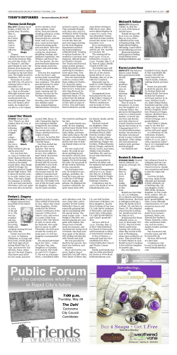


© Copyright 2026