1. technology and computing
2. software
3. databases

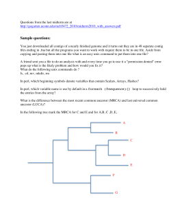
Manual/Tutorial
Last updated: 06 October 2014
Contact: Michael Hackenberg ([email protected])
Table of Contents
INTRODUCTION
6
MAIN FEATURES
6
2 GETTING STARTED
7
2.1 DEPENDENCIES
7
2.2 INSTALL THE DATABASE
7
2.3 POPULATE THE DATABASE
8
2.3.1 GENOME SEQUENCES
8
2.3.2 MICRORNAS LIBRARIES
8
2.3.3 OTHER SMALL RNA SPECIES
9
2.3.4 SRNABENCH HELPER TOOLS
9
2.4 QUICK START
9
2.4.1 LIBRARY MAPPING MODE
10
2.4.2 GENOME MAPPING MODE
11
2.4.3 PREDICTION OF NOVEL MICRORNAS
11
2.4.4 USING OTHER LIBRARIES
12
2.4.5 DETECTING ISOMIRS
12
2.4.6 VISUALIZING ALIGNMENTS
13
3 SRNABENCH PARAMETERS
13
3.1 MANDATORY PARAMETERS
13
3.2 MAPPING PARAMETERS
14
3.3 ANALYSIS TYPES AND LIBRARIES
14
3.4 ADAPTER TRIMMING AND PRE-PROCESSING
16
3.5 PROFILING PARAMETERS
17
3.6 OUTPUT OPTIONS
18
3.7 PROGRAM NAMES
19
3.8 PREDICTION OF NOVEL MICRORNAS
19
4 WORK-FLOW
20
4.1 ANALYSIS STEPS
20
4.1.1 GENOME MODE
20
4.1.2 LIBRARY MODE
21
4.2 ISOMIR SPECIFICATION
21
4.3 PREDICTION OF NOVEL MICRORNAS
22
5 OUTPUT FILES
24
5.1 EXPRESSION PROFILING
24
5.1.1 *.GROUPED FILES
24
5.1.2 SINGLE ASSIGNMENT FILES: *_SINGLEA.GROUPED
25
5.2 MICRORNA SPECIFIC OUTPUT
26
5.2.1 MIRBASE_MAIN.TXT
26
5.2.2 HAIRPIN_NOVELSTAR.TXT
26
5.2.3 HAIRPIN_SUSPICIOUS.TXT
27
5.3 ISOMIR OUTPUT
27
5.3.1 MIRBASE_ISO.TXT
27
5.3.2 ISOMIR ANNOTATION
28
5.3.3 PER MATURE MICRORNA ISOMIR SUMMARY
29
5.3.4 ISOMIR SUMMARY
29
5.4 GENERAL INFORMATION
30
5.4.1 THE “READS.ANNOTATION” FILE
30
5.5 THE ’STAT’ FOLDER
31
5.5.1 READ LENGTH
31
5.5.2 MAPPING SUMMARY
32
5.6 ALIGNMENT FILES - PROCESSING PATTERN
32
5.7 NOVEL MICRORNAS
33
6 TIPS AND TRICKS
34
6.1 OVERWRITE THE MAPPING PARAMETERS
34
6.2 USING BOWTIE INDEXES AS LIBRARIES IN GENOME MODE
34
6.3 MULTI-SPECIES ANALYSIS
35
6.4 CONSTRUCTION OF SHARED LIBRARIES
35
6.5 PREDICTION OF NOVEL MICRORNAS
36
6.6 PROFILE TRNAS
36
7 DIFFERENTIAL EXPRESSION
36
7.1 MANDATORY PARAMETERS
36
7.2 ANALYSIS TYPES
37
7.3 DIFFERENTIAL EXPRESSION
38
7.4 ISOMIR ANALYSIS
38
7.5 READ LEVEL ANALYSIS
39
8 DIFFERENTIAL EXPRESSION OUTPUT
40
8.1 DIFFERENTIAL EXPRESSION OUTPUT
40
8.1.1 NOMENCLATURE OF DIFFERENTIAL EXPRESSION OUTPUT FILES
40
8.1.2 *.EDGER FILES
40
8.1.3 *.EXTEDGER FILES
41
8.2 EXPRESSION MATRIX
41
8.3 DIFFERENTIAL ISOMIR PATTERN
41
8.3.1 *.TTEST AND *.SIG FILES
42
8.3.2 SEQUENCING STATISTIC
42
20 June 2014
1 Introduction
sRNAbench is a free web-server tool and standalone application for processing smallRNA data obtained from next generation sequencing platforms, such as Illumina or
SOLiD. The sRNAbench tool is the replacement for miRanalyzer.
Main features

The expression levels of small RNAs can be profiled in two different ways
(depending on whether a good genome sequence/annotation is available or not):
i) mapping the reads against the genome and obtaining the expression levels by
means of fasta, gtf/gff or bed format annotations or ii) mapping against sequence
libraries in fasta/Bowtie index format (as it is done by miRanalyzer).

An unlimited number of genomes can be used in the analysis at the same time
without having to pool all sequences into a single file/Bowtie index. This feature
is especially important when analysing the interaction between parasites and
hosts, symbiosis or virus infected cells.

Adapter and barcode trimming can be performed.

sRNAbench accepts fastq, fastq.gz, sra, read count and fasta input format.

Extensive profiling of all microRNA sequences and length variants (isomiRs).
Furthermore, NTAs (non-templated additions) can be detected for all sequenced
libraries and not only for microRNAs.

Several statistics and graphical summaries are available.

The prediction of novel microRNAs was improved compared to miRanalyzer,
being more specific now. The prediction is based on structural, sequence and
biogenesis features.

Detection of differentially expressed microRNAs (including novel microRNAs)
and differences in the isomiR pattern.
sRNAbench can be used through its web-server instance, in this case consult the web
manual. However, the web application has some limitations like the restricted number
of configurable parameters and the limited number of available genome assemblies.
Therefore, to cover all possible analysis and user requirements, sRNAbench can also be
6
20 June 2014
installed locally. This tutorial will help the user during the local installation and will try
to be a guide during the entire small-RNAs analysis.
2 Getting started
2.1
Dependencies
sRNAbench is implemented in JAVA and apart from a JRE, it needs the following third
party software that must be installed in the PATH.

Vienna RNA package for RNA Secondary Structure Prediction and Comparison
(Vienna package 2). sRNAbench will only work with Vienna 2.0 or higher.

Bowtie - An ultra-fast memory-efficient short read aligner (Bowtie). sRNAbench
will only work with Bowtie1.

Only for the differential expression module some other software must be
installed: R package, Bioconductor, edgeR package and for some specific
analysis The Apache Commons Mathematics Library.
2.2
Install the database
sRNAbench relies on a local database where most of the library files, genome sequences
and Bowtie indexes must be stored. The database can have any arbitrary name and the
easiest way to generate it, is by means of the “start-up” database:
1. Download the “start-up” database: sRNAbenchDB and extract it to a directory of
your choice: ‘tar -xvzf sRNAbenchDB.tgz’. To populate the database, please
check 2.3
Populate the database.
NOTE: “start-up” database only includes genome and microRNA sequences for
human, human herpes virus type 8 (HHV-8) and Epstein-Barr virus (EBV) microRNAs.
2. Download the most recent version and replace the sRNAbench.jar file from the
database.
3. Only for differential expression module: Download the most recent version of
7
20 June 2014
sRNAbenchDE.jar and place it into the database.
Once the “start-up” database has been installed, the user should see the following
folders within the database folder selected:

libs: default location for all sequence libraries except the genome sequences.

index: contains the Bowtie indexes of the genome sequences.

seqOBJ: contains the genome sequences objects generated by makeSeqObj
program.

out: default output folder.
2.3 Populate the database
2.3.1 Genome sequences
In order to add a genome sequence to the database, two steps are needed:
1. Generate the genome bowtie index, by means of the ’bowtie-build’ software, and
place it into the index folder of the sRNAbenchDB.
2. Process the genome sequence(s) with makeSeqObj and place the obtained zip
file into the seqOBJ folder.
EXAMPLE: java -jar makeSeqObj.jar hg19.fa.
NOTE: this step might take a while (hours) in case of big genomes. Furthermore, it is
quite memory demanding, so probably the heap space needs to be increased by means
of -Xmx on the command line.
2.3.2 microRNAs libraries
To our knowledge, the best source for known microRNA sequences is miRBase. In
order to include the miRBase libraries to sRNAbench, download the mature and hairpin
sequences and extract them into the libs folder of the sRNAbench database.
NOTE: in unix systems, to download the libraries, move to the libs folder and type: ‘wget -nd
8
20 June 2014
ftp://mirbase.org/pub/mirbase/CURRENT/mature.fa.gz’ and ‘wget -nd
ftp://mirbase.org/pub/mirbase/CURRENT/hairpin.fa.gz’.
NOTE: both, mature microRNA and pre-microRNA (hairpin) annotations need to be included.
Currently, only fasta input format with the miRBase nomenclature is supported (fasta ids
starting with the short species name ’hsa’, ’mmu’, ’ath’, etc..) .
2.3.3 Other small RNA species
Other small RNA annotations can be provided either in fasta format, Bowtie index
format or bed format. BED format will be only valid if the genome sequence is
specified with species (see below 3.3
Analysis types and libraries). If no extension is
provided, sRNAbench will assume the existence of a Bowtie index in the libs folder and
will try to align directly against it. Otherwise, for a library with fa extension either the
coordinates are obtained by mapping the sequences against the genome sequence (if
species is set) or a Bowtie index is generated first by sRNAbench.
NOTE: the bed format annotations must be from the same genome sequence assembly.
2.3.4 sRNAbench helper tools
Some helper tools have been developed in order to facilitate the usage of Ensembl and
NCBI annotations. The helper tools can be accessed here.
2.4 Quick start
The “start-up” database contains an example dataset obtained from Gottwein et al. This
dataset was obtained from primary effusion lymphoma cell line BC-1 (human) which is
infected by two viruses: human herpes virus type 8 (HHV-8) and Epstein-Barr virus
(EBV). This dataset shows one of the main strengths of sRNAbench, the possibility to
analyse multi-species assays. Next, we will illustrate the use of sRNAbench by means of
some examples:
9
20 June 2014
2.4.1
Library mapping mode
First of all, we will align the input dataset to miRBase libraries for the three species:
‘java -jar sRNAbench.jar dbPath=/path2DB/sRNAbenchDB microRNA=hsa:ebv:kshv
input=SRR343332.fa.gz’
NOTE: If the output folder is not provided, the program will write the results into
‘sRNAbenchDB/out/SRR343332/’.
Next, some output files that you might be interested in will be explained (for the rest
please see 5

Output files):
reads.fa and reads_orig.fa: reads.fa contains all unmapped reads (after the run
has finished), while reads_orig.fa contains the initial set of reads.

hairpin_sense.grouped: the expression profiling of known pre-microRNAs.

mature_sense.grouped: the expression profiling of known mature microRNAs.

mature_sense_singleA.grouped: a single read assignment expression profiling
of mature_sense.grouped. The single read assignment (each read is only
assigned to one locus) is explained below.

hairpin_sense_singleA.grouped: a single read assignment expression profiling
of hairpin_sense.grouped. Only those reads that are not derived from mature
microRNAs do count.

miRBase_main.txt: profiling of known microRNAs at a pre-microRNA level.
This file includes the read counts for the canonical version (by default, those
defined by miRBase).

hairpin_NovelStar.txt: mature microRNA sequences that correspond to the
’arms’ that have not been reported before (are not included in miRBase)

reads.annotation: annotation of all reads, i.e. to which libraries the reads have
been mapped.

hairpin_suspicious.txt: pre-microRNA sequences that failed the consistency
test (either they have no stem-loop or one of the mature sequences folds back
onto itself).

short_reads.txt: reads filtered out due to minimum length.
10
20 June 2014

in stat folder Read Length: the read count as a function of read length.

in stat folder mapping summary: a summary statistics of the small RNAs
mapped.

in stat folder microRNA_species.txt: the distribution of mature microRNAs
over the species.

in stat folder hairpin.len: the length distribution of the hairpin mapped reads
(only forward strand).
2.4.2 Genome mapping mode
The same analysis carried out in 2.4.1
Library mapping mode, can also be performed
by means of the genome mapping mode.
NOTE: the default database only includes human chromosome 22, and therefore only the
microRNAs located on this chromosome can be profiled.
‘java -jar sRNAbench.jar dbPath=/path2DB/sRNAbenchDB microRNA=hsa:ebv:kshv
species=chr22:NC_007605:NC_009333 input=SRR343332.fa.gz
output=/path2DB/sRNAbenchDB/out/genome’
Compared to the library mapping mode, there are only minor differences on the
number of output files:

readsNotAssigned.fa: contains the reads that have been mapped to the genome,
but not assigned to any reference sequence.

in stat folder Read length: the length distribution of genome mapped reads.

in stat folder: the genome mapping mode retrieves the length distribution also
for antisense mapped reads.
2.4.3 Prediction of novel microRNAs
The prediction of novel microRNAs can be activated setting up predict=true:
‘java -jar sRNAbench.jar dbPath=/path2DB/sRNAbenchDB microRNA=hsa:ebv:kshv
species=chr22:NC_007605:NC_009333 input=SRR343332.fa.gz
11
20 June 2014
output=/path2DB/sRNAbenchDB/out/genome predict=true’
Additional output files:

novel.txt: Summary of novel microRNAs.

mature_novel.fa and hairpin_novel.fa: mature and pre-microRNA sequences.

folder novel: contains the alignments to the novel pre-microRNA sequences.
2.4.4 Using other libraries
Other libraries can be analysed setting libs=’library name’. If the library is provided in
fasta format, sRNAbench will first generate a bowtie index of this file. Otherwise, the
library will be mapped to the genome in order to obtain the chromosome coordinates of
the reference sequences.
WARNING: In genome mode, only unspliced reference sequences should be provided in fasta
format. Spliced genes should be provided as bowtie indexes or in bed or gtf/gff format (see 2.3.3
Other small RNA species and 6.2 Using bowtie indexes as libraries in genome mode).
‘java -jar sRNAbench.jar dbPath=/path2DB/sRNAbenchDB microRNA=hsa:ebv:kshv
input=SRR343332.fa.gz libs=hg19-tRNAs.fa’
Additional output files:

hg19-tRNAs_sense.grouped and hg19-tRNAs_antisense.grouped: reads
mapped to the sense and antisense strands of the hg19-tRNA.fa library.
2.4.5 Detecting isomiRs
IsomiRs can be detected adding isoMiR=true:
‘java -jar sRNAbench.jar dbPath=/path2DB/sRNAbenchDB microRNA=hsa:ebv:kshv
input=SRR343332.fa.gz libs=hg19-tRNAs.fa isoMiR=true’
12
20 June 2014
Additional output files:

miRBase_iso.txt: the isomiR information for each mature microRNA

isomiR annotation: (miRBase_isoAnnotation.txt) the isomiR annotation at read
level.

in stat folder, per mature microRNA isomiR summary
(isomiR_summary.txt): the number of reads found for the different isomiR types
for each of the mature microRNAs.

in stat folder, isomiR summary: sample wide summary as a function of isomiR
type.

in stat folder, miRBaseNTA_lenNTA.txt: summary of non-templated additions
as function of ’addition length’ (for example 1, 2, 3, etc… As added)
2.4.6
Visualizing alignments
The alignments of the microRNAs can be generated setting plotMiR=true:
‘java -jar sRNAbench.jar dbPath=/path2DB/sRNAbenchDB microRNA=hsa:ebv:kshv
input=SRR343332.fa.gz plotMiR=true’
Additional output files:

Alignment files - processing pattern (hairpin folder): holds the alignment files.
3 sRNAbench parameters
The parameters are provided using the following form: parameter=value. For example
to specify the mandatory path to the local database: dbPath=/home/usr/...
3.1

Mandatory parameters
dbPath: the full path to the sRNAbench database (for example:
‘/home/user/sRNAbenchDB/’).
13
20 June 2014

input: the path to the input file (fastq, sra, read/count, fasta, or sRNAbench fasta
format).
3.2
Mapping parameters
The following parameters are passed to the Bowtie aligner. For more information, please
see the Bowtie manual page.

noMM <int>: number of mismatches (default: noMM=1).

seed <int>: the length of the seed, -l parameter in Bowtie (default: seed=19).

alignType [n,v]: the alignment type, can be either ’n’ (-n parameter in Bowtie,
i.e. alignType=n) or ’v’ (-v parameter in Bowtie, i.e. alignType=v). Note that
when setting ’v’, the seed parameter will have no effect and Bowtie will try to
align the entire read. Briefly, ’n’ will perform a seed alignment (only the first
nucleotides are used for the alignment, i.e. mismatches outside the seed region
do not count).
NOTE: To detect isomiRs, ’n’ must be used.

mBowtie <int>: maximum number of allowed multiple mappings, -m parameter
in Bowtie (default: mBowtie=40).

p <int>: “Launch <int> parallel search threads” -from Bowtie manual(default: p=4).

chunkmbs <int>: “The number of megabytes of memory a given thread is given
to store path descriptors in --best mode” -from Bowtie manual- (default:
chumkmbs=128).
3.3

Analysis types and libraries
solid <Boolean>: if it is set to true, SOLiD input data is expected (default:
solid=false).

microRNA <species list>: microRNA species that should be used for the
analysis. An arbitrary number of species can be used, the short species names
14
20 June 2014
must be provided separated by ’:’.
EXAMPLE: microRNA=hsa:ebv will map the input reads simultaneously to human
(hsa) and Epstein-Barr virus (ebv) microRNAs.

species <genome assembly list>: genome sequences that will be used. An
arbitrary number of different genome sequences can be used, the names must be
provided separated by ’:’.
EXAMPLE: species=hg19_5:NC_007605 will map the input reads simultaneously to
hg19_5 (in this case, hg19_5 is the Bowtie index abbreviation for the human genome
version hg19/NCBI37 path 5 genome sequence) and the Epstein-Barr virus genome
sequence.
NOTE: Bowtie indexes for the genome sequences must be located within the
sRNAbench database index folder.

mature <String>: name of the library that holds the mature microRNAs (for
example mature.fa for miRBase library) (default: mature=mature.fa).

hairpin <String>: name of the microRNA precursor sequences (for example
hairpin.fa for miRBase library) (default: hairpin=hairpin.fa).

libs <String>: name of the library file. Typically, these files would hold other
types of small RNAs like tRNA, snoRNA, snRNA, piRNA, rRNA, yRNA,
vaultRNA, etc…
NOTE: If a name is given, the program will search for the file in the default
sRNAbench database folder (libs), however if a full path is given the program will use
this file, which then does not need to be within the sRNAbench database. The files can
be provided in fasta format, bed format or directly as Bowtie indexes.

homolog <species list>: a string of short species names separated by ‘:’,
indicating those species that should be used for homologous based microRNA
detection.
EXAMPLE: homolog=mmu:rno would map the reads (after profiling known
microRNAs) to the hairpin sequences of mouse and rat, in order to detect putative novel
15
20 June 2014
microRNAs based on homology.
NOTE: homolog=all will use all species except those provided on microRNA species
list.

noGenome <boolean>: if a genome sequence is provided (species) and
noGenome is set to true, then the program will execute both types of analysis: 1)
genome sequence based and 2) sequence libraries based.
NOTE: if species is not provided, sRNAbench will try to align against sequence
libraries directly and not to the genome. In this case, bed file format is not supported.
3.4

Adapter trimming and pre-processing
adapter <String>: the adapter sequence. If the adapter is not provided, then the
input is assumed to be adapter trimmed.

adapterStart <int>: position (0-based coordinates) in the read where the
adapter search will start (default: adapterStart=0).

adapterMinLength <int>: minimum length of the adapter to be detected
(default: adapterMinLength=10).

adapterMM <int>: maximum number of mismatches allowed between the
adapter sequence and the read (default: adapterMM=1).

removeBarcode <int>: eliminates the first <int> bases from the 5’ end of the
read (default: removeBarcode=0).

recursiveAdapterTrimming <boolean>: recursively search for the adapter at
the
3’
end,
without
considering
adapterMinLength
(default:
recursiveAdapterTrimming=false).
NOTE: This function might be activated for read length 36, if sRNA populations of
length between 27 and 34 should be analysed.

holdNonAdapter <boolean>: include the reads where the adapter sequence was
not found (default: holdNonAdapter=false).

writeNonAdapter <boolean>: write out the reads where the adapter was not
16
20 June 2014
found (default: writeNonAdapter=false).

guessAdapter <boolean>: the program tries to guess the adapter. Briefly,
sRNAbench will align the first 250.000 reads to the genome using the Bowtie
seed function (the adapters will not count for the mismatches). Then, the adapter
sequence is defined as the most frequent 10-mer starting at the first mismatch
(default: guessAdapter=false).

maxReadLength <int>: maximum length of input reads (filters out all reads
that are longer than <int>, by default this filter is not applied).

minReadLength <int>: minimum read length of input reads (filters out shorter
reads than <int>, default: minReadLength=15).

minRC <int>: minimum read count (filters out reads with less count than <int>,
default: minRC=1).

sep <String>: if the input is a fasta file, this parameter allows to indicate which
character separates the ’ID’ and the ’Read Count’. For example: >1-45798
(ID=1, Read Count = 45798), then the separate character will be set as sep=-.
Default: sep=#

libsFilter=<String>: name of the library file that should be used to filter out
certain reads (for example those that map to ribosomal RNA fragments). Fasta
format and bowtie index is accepted.
3.5
Profiling parameters
There are several parameters that could influence the profiling of known elements.

winUpMiR <int>: the upstream flanking for the detection of microRNAs
(default: winUpMiR=3).

winDownMiR <int>: the downstream flanking for the detection of microRNAs
(default: winDownMiR=5).
EXAMPLE: hsa-miR122-3p maps to the ’+’ strand of chr18 at start position 56,118,356
and end position 56,118,377. Then, this region is extended adding the downstream and
upstream flanks: from 56,118,356-winUpMiR to 56,118,377+winDownMiR. Therefore, all
the reads that lie within this region are assigned to the reference element (hsa-miR122-3p
17
20 June 2014
in this case).

winUpTrans <int>: same as winUpMiR, but applied to libs reference sequences
(default: winUpTrans=0).

winDownTrans <int>: same as winDownMiR, but applied to libs reference
sequences (default winDownTrans=0).

hierarchical <boolean>: Apply a hierarchical classification. hierarchical=true:
mapped reads cannot map again, i.e. are removed after mapping (like it is done
in miRanalyzer). If hierarchical=false, then reads can map to multiple libraries
(default: hierarchical=true).

base <0,1>: coordinates format of bed input files, 0-based or 1-based (default:
base=0).

matureMM <int>: number of allowed mismatches between the genome and the
known mature microRNA. This parameter influences the genome coordinate
detection of known microRNAs (default: matureMM=0).

hairpinMM <int>: number of allowed mismatches between the genome and the
known pre-microRNA sequence. This parameter influences the genome
coordinate detection of known pre-microRNAs (default: hairpinMM=0).

matureHomologMM <int>: number of allowed mismatches between the
putatively
homologous
microRNA
and
the
genome
(default:
matureHomologMM=2).

isomiRseed <int>: number of 5’ nucleotides which are not used to detect nontemplated additions (NTAs) (default: isomiRseed=18).
3.6

Output options
plotMiR <boolean>: plot out the microRNA alignments to the hairpin folder
(default: plotMiR=false).

plotLibs <boolean>: plot out the alignments against the libraries provided by
libs (default: plotLibs=false).

minRCplotLibs <int>: minimum read-count in order to write out the libs
alignment file (default: minRCplotLibs=200).

minRCplotMiR <int>: minimum read-count in order to write out the
18
20 June 2014
microRNA alignment file (default: minRCplotMiR=20).

isoLibs <boolean>: detect non-templated additions for libs (default:
isoLibs=false).

isoMiR <boolean>: profile and classify isomiRs (default: isoMiR=false).

maxLenForSecStruc <int>: the secondary structure is calculated if the length
of the reference sequence <= <int>, it only works if plotLibs=true and the readcount of the sRNA >= minRCplotLibs (default: maxLenForSecStruc=200).

fullIsoStat <boolean>: writes out a full isoMiR statistic, as a function of the
different species, 3p and 5p (default: fullIsoStat=false).

tRNA <String>: if a genomic tRNA library is used, tRNA mappings will be
summarized by anticodons. The value must be the same library set with libs.

writeGenomeDist <boolean>: writes out a mapping statistic as a function of
chromosome (default: writeGenomeDist=false).

graphics <boolean>: sRNAbench generates graphic files, R/ggplot2 must be
installed –execute ‘install.packages("ggplot2")’ in your R workspace - (default:
graphics=false).
3.7

Program names
RNAfold <String>: name of the RNAfold program. For example, if both
Vienna 2.0 and Vienna 1.8.5 or before are installed on the computer (default:
RNAfold=RNAfold).
3.8

Prediction of novel microRNAs
predict <boolean>: prediction of novel microRNAs. The prediction is
deactivated by default predict=false.

kingdom [animal,plant]: the microRNAs dataset kingdom must be indicated, in
order to use the appropriate feature thresholds (default: kingdom=animal).

maxClusterDist <integer>: the maximal distance between two read clusters.
By default maxClusterDist= 60 (animal) and maxClusterDist=180 (plant).

ForceHomolog <boolean>: if homolog and microRNA are not set, all known
19
20 June 2014
microRNAs (miRBase) are used to assign a name to the novel microRNAs by
means of sequence similarity (default: ForceHomolog=true).

novelStrict <boolean>: discards non bona fide microRNAs (default:
novelStrict=true).

novelName <String>: species short name used for the novel microRNAs. For
example, hsa (human), mmu (mouse), rno (rat), etc... (default: novelName=new).

seedFamily <int>: length of the seed region used to determine members of a
family (default: seedFamily=8).

seedFamilyMM <int>: number of mismatches allowed within the seedFamily
(default: seedFamilyMM=0).
4 Work-flow
4.1
Analysis steps
sRNAbench can be used in two different modes: Genome mode and Library mode. Both
modes share common pre-processing steps which consist on i) adapter trimming, ii)
rudimentary quality control (remove reads with Ns), iii) collapse identical reads into one
unique entry assigning a read count (number of times a given read was obtained in the
experiment). Moreover, both modes can be carried out in a hierarchical (by default) or
non-hierarchical way (a read can be assigned to several libraries) way. Hierarchical
means that each read that maps to a given library is removed from the analysis and
therefore cannot map again to another library (each read can only map to one annotation
group). The group mapping order is: 1) MicroRNAs (microRNA), 2) putative
homologous (homolog), 3) other libraries (libs).
NOTE: an unlimited number of libs can be provided and they will be used in the order as they
appear on the command line.
4.1.1 Genome mode
When a genome sequence is provided at the command line (species), then all reads are
20
20 June 2014
first mapped to this genome. Afterwards, the genome coordinates of the reference small
RNA annotations (microRNAs and those given by libs) are determined. For fasta
annotations, the sequences are mapped to the genome and the chromosomal coordinates
are retrieved in BED format. If the annotation input is given in BED format, the
corresponding coordinates are adopted directly.
4.1.2
Library mode
If no genome sequence is available, sRNAbench proceeds nearly identical as
miRanalyzer does. Instead of mapping to the genome sequence, the reads are
successively mapped first to the microRNA annotation and after this to the libraries
provided by libs.
4.2
IsomiR specification
sRNAbench does not only detect the canonical (miRBase) microRNA sequence, but also
all isomiRs (sequence variants). Frequently, a microRNA can show different posttranscriptional modifications. For example, it can be 3’ trimmed and adenylated. In
order to keep a simple classification schema, sRNAbench uses a hierarchical
classification for these isomiRs, basically for each read is tested if it belongs to one of
the following five classes:
1) The read is identical to the canonical sequence (miRBase entry).
2) The read starts and ends at the same position as the canonical sequence in the premicroRNA, but it shows sequence variations (most likely due to sequencing errors,
but RNA editing events and SNP might exist as well).
3) The read has non-templated additions (A, T(U), C or G added to its 3’ or 5’ end),
i.e. nucleotides at the 3’ end that do not match with the reference (template).
4) The read starts or ends at the same position as the canonical version. For this case
we can distinguish 4 groups:
a) 3’ trimmed read: the read starts at the same position as the canonical sequence
(same 5’ end) but it is shorter.
b) 3’ extended read: the read starts at the same position as the canonical sequence
21
20 June 2014
(same 5’ end) but it is longer and maintains the template nucleotides.
c) 5’ trimmed read: the read ends at the same position as the canonical sequence
(same 3’ end) but it is shorter.
d) 5’ extended read: the read ends at the same position as the canonical sequence
(same 3’ end) but it is longer and maintains the template nucleotides.
5) The read does coincide neither in 5’ nor in 3’ with the canonical sequence (multiple
length variant).
Figure 1: The figure shows the hierarchical isomiR classification used in sRNAbench.
4.3
Prediction of novel microRNAs
The implemented microRNA prediction method has been used before to detect novel
microRNAs in plants (Hackenberg et al.). Briefly:

The reads are mapped to the genome sequence

Reads that map to nearly identical positions in the genome are clustered into
’read clusters’ in the following way:
i) The reads are sorted by read count (read frequency).
ii) The most frequent read is chosen to form the first read cluster. Note that, the
22
20 June 2014
cluster coordinates are adopted from this most frequent read.
iii) The rest of the reads are checked to lie within a window defined by
‘clusterStart – 3 nt’ and ‘clusterEnd + 5 nt’ on the same strand (flanks were
added in order to assign all possible isomiRs to their read cluster).
iv) if the read belongs to an existing cluster, the read information (sequence and
the read count) is added to the cluster.
v) if the read does not belong to an existing cluster, a new cluster is opened.

After clustering all reads, read clusters with distances of less than 180 nt for
plants and less than 60 nt for animals are chosen. The bona fide miRNAs should
have two read clusters corresponding to the two arms processed from the premicroRNA sequence.

Last, the genomic sequence spanned by the two read clusters is extracted and its
secondary structure and alignment pattern of the derived pre-miRNA is
analysed. Then, the retained read cluster must:
i) Map to the stem of the putative pre-miRNA.
ii) Not fold back onto itself (i.e. it is not spanning the loop region).
iii) Be above all calculated feature thresholds shown in ¡Error! No se
encuentra el origen de la referencia..
23
20 June 2014
Figure 2: Features used in the prediction of novel microRNAs. The thresholds have been determined
using the same training set as described before miRanalyzer. They represent the percentile 5 (P5) of the
distributions obtained for known microRNAs for the high confidence prediction (HC) and 0.5 for the low
confidence prediction (LC).
5 Output files
5.1
Expression profiling
5.1.1 *.grouped Files
These files contain the expression profiling of the annotation provided:
1) name: name of the element.
2) unique reads: number of unique reads mapped to this element.
24
20 June 2014
3) read count: total number of reads mapped to this element.
4) read count (mult. map. adj.): each read is divided by the number of times it mapped
either to different genome loci (genome mode) or sequences in the library (sequence
library mode).
5) RPM (lib): Reads Per Million normalized by the total number of reads mapped to
the library.
6) RPM (total): Reads Per Million normalized by the total number of reads mapped to
the genome (genome mode) or by the total number of reads in the analysis
(sequence library mode).
7) chromosome string (only for genome mappings): the chromosome string has the
following format: “chromosome#chromosome start#chromosome end#strand”, it
refers to the genome position of the annotation.
NOTE: these coordinates are generated by sRNAbench if the annotation input is a fasta
file, and they are taken from the annotation file if the input is a BED or GTF/GFF file.
5.1.2 Single Assignment Files: *_singleA.grouped
These files contain an expression profiling based on a single assignment of the reads,
i.e. each read is only assigned once (to a locus or reference element). It is generated
using *.grouped file and the read.annotation file in the following way:
1) *.grouped files are sorted by read count.
2) Going from the most expressed microRNA (or other ncRNA) to lower expressed
ones, the reads that map to the reference sequence are summed and removed before
moving to the next microRNA. In this way, each read is uniquely assigned to one
reference sequence (the one with the highest total expression value).
NOTE: *_ singleA files are first generated for sense mappings, this means that a read that
maps to both, the sense and the antisense orientation is only assigned to the sense orientation.
WARNING: this file should not be used for differential expression analysis.
25
20 June 2014
5.2
MicroRNA specific output
5.2.1 miRBase_main.txt
This file contains a summary at the pre-microRNA level. Only microRNAs that have a
suitable secondary structure (stem-loop) and a mature sequence that do not fold back
onto itself are listed.
1) name: microRNA name.
2) UR: number of unique reads mapped to the pre-microRNA.
3) RC: total number of reads mapped to the pre-microRNA.
4) RC (adj.): adjusted read count (see 5.1.1
*.grouped Files).
5) UR5p: number of unique reads mapped to the 5’ arm.
6) RC5p: total number of reads mapped to the 5’ arm.
7) RC5p (adj.): adjusted read count of the 5’ arm.
8) name-5p: name of the 5’ arm.
9) UR3p: number of unique reads mapped to the 3’ arm.
10) RC3p: total number of reads mapped to the 3’ arm.
11) RC3p (adj.): adjusted read count of the 3 arm.
12) name-3p: name of the 3’ arm.
13) coordinates:
coordinate
string
id,
like:
chr1:hsa#198828173#198828282#
(“chromosome#chromosome start#chromosome end#strand”).
14) 5pcanonical: read count of the 5p arm ’canonical’ sequence.
15) 3pcanonical: read count of the 3p arm ’canonical’ sequence.
5.2.2 hairpin_NovelStar.txt
This file holds those mature microRNA sequences that are detected in the dataset, but
are not present in the annotation (miRBase). The sequences included must form a
Drosha/Dicer (DCL) compatible dsRNA with the annotated mature microRNA (1-2 nt
3’ overhang).
1) name: name of the “novel” mature microRNA.
26
20 June 2014
2) sequence: sequence of the “novel” mature microRNA.
3) read count: read count.
5.2.3 hairpin_suspicious.txt
This file lists all microRNA sequences present in the annotation database (normally
miRBase), for which any kind of error is detected (if plotMiR=true, these sequences are
written out to the hairpin_error folder).
1) name: microRNA id.
2) chromosome: chromosome.
3) start: chromosome start.
4) end: chromosome end.
5) strand: orientation.
5.3
isomiR output
5.3.1 miRBase_iso.txt
This file holds the isomiR composition for each mature microRNA. The file has the
following columns:
1) name: name of the mature microRNA.
2) pre-microRNA: name of the precursor sequence.
3) RC: read count of the mature sequence (canonical sequence and all isomiRs).
4) UR: unique reads mapped to the mature sequence (canonical sequence and all
isomiRs).
5) RPM (lib): Read Per Million normalized by the total number of reads mapped to the
library.
6) RPM (total): Reads Per Million normalized by the total number of reads mapped to
the genome (genome mode) or the total number of reads in the analysis (sequence
library mode).
7) arm: microRNA arm (either 3p or 5p).
8) isoString: this string holds the information for all detected isomiRs. The information
27
20 June 2014
for each isomiR is separated by ’|’. For decoding the string please see these
examples:
o nta#BASE_RC: all non-templated nucleotide additions.
EXAMPLE: nta#A_9568, means that 9,568 reads in the sample present one or
more 3’ terminal As, which are not present in the reference sequence (either
genome or miRBase hairpin sequence).
o nta#BASE#ADDITIONS_RC: non-templated nucleotide additions of a
given length.
EXAMPLE: nta#T#1_125, means that 125 reads present mono-uridylation at its 3’
end (1 U added, which is not present in the reference sequence).
o lv5p_RC: 5’ length variants.
EXAMPLE: lv5p_862 means that 862 reads show any type of 3’ length variation..
o lv3p_RC: 3’ length variants.
EXAMPLE: lv3p_222835 means that 222835 reads do show any type of 3’ length
variation.
o mlv_RC: Multiple length variants.
5.3.2
isomiR annotation
The file miRBase_isoAnnotation.txt assigns to each read mapped to a known microRNA
an isomiR related label.
1) read: read sequence.
2) name: name of the mature microRNA.
3) preMicro: name of the pre-microRNA.
4) isoClass: assigned isomiR class.
5) NucVar: observed nucleotide variation (reference > sample).
28
20 June 2014
6) read count: read count.
5.3.3 per mature microRNA isomiR summary
An isomiR summary for each of the mature microRNAs detected:
1) name: name of the mature microRNA.
2) UR: number of unique reads.
3) RC: read count.
4) RPM(total): Reads Per Million normalized to all pre-processed input (library
mapping)/genome mapped (genome mode) reads.
5) RPM(lib): Reads Per Million normalized to all reads mapped to a known
microRNA.
6) Canonical_RC: read count of the canonical sequence.
7) NTA(A): number of reads with a non-templated A addition.
8) NTA(U): number of reads with a non-templated U addition.
9) NTA(C): number of reads with a non-templated C addition.
10) NTA(G): number of reads with a non-templated G addition.
11) lv3pE: number of reads with 3’ length extension (longer than the canonical
sequence).
12) lv3pT: number of reads with 3’ length trimming (shorter than the canonical
sequence).
13) lv5pE: number of reads with 5’ length extension (longer than the canonical
sequence).
14) lv5pT: number of reads with 5’ length extension (shorter than the canonical
sequence).
15) mv: number of reads classified as multiple length variants.
5.3.4
The
isomiR summary
summary
is
composed
of
two
files:
“miRBase_allNTA.txt”
and
“miRBase_otherVariants”, which summarize all the isomiR statistics for NTA (nontemplated additions) and several length variants.
29
20 June 2014
1) name: the name of the isomiR type:
a) A (adenine addition), C (cytosine addition), T (U/T addition), G (G addition).
b) lv5pT: 5’ trimmed.
c) lv5pE: 5’ extended.
d) lv5p: 5’ length variant (lv5pT + lv5pE).
e) lv3pT: 3’ trimmed.
f) lv3pE: 3’ extended.
g) lv3p: 3’ length variant (lv3pT + lv3pE).
h) mv: multiple length variants.
2) totalRC: number of reads mapped to microRNAs.
3) NTA_count: number of reads that belong to a given isomiR type.
4) wMean: weighted mean (NTA_count/totalRC).
5) mean: mean isomiR ratio of the sample. For each microRNA, an isomiR ratio is
calculated: (number of reads belonging to a certain isomiR type) / (total number of
reads mapped to the microRNA).
6) stdDev: standard deviation of the mean.
5.4
General information
5.4.1
The “reads.annotation” file
This file contains a summary at the read level, i.e. each read is listed individually
together with all the annotations to which it mapped. It contains the following columns:
1) read sequence.
2) the read count.
3) Reads Per Million normalized by the total number of reads mapped to the genome
(genome mode) or the total number of reads in the analysis (sequence library mode).
4) Classification. It consists on the name of the annotation file (for libs) or
hairpin/mature (microRNAs from miRBase), plus the mapping orientation (sense or
anti-sense). The format is “AnnotationGroup#Orientation”.
30
20 June 2014
NOTE: the name can be “mixed” if the read maps to several different annotations.
5) Mapped Annotations. This column contains all the annotations to which the read has
been
aligned.
The
format
“AnnotationGroup#AnnotationName#Orientation#Chromosome
is:
position”.
The
chromosome position is only applicable in the genome mode, for library mode the
chromosome is set to’s’. The several different annotations to which a read can map
are separated by ’$’.
EXAMPLE:
“hv_030312_v2_18#MLOC_55934.3#antisense#s$hv_030312_v2_18#MLOC_55933.2#sen
se#s” means that i) the corresponding read mapped twice (two annotation strings separated
by ’$'), ii) the read maps to one gene in sense direction and another one in antisense
direction, iii) “hv_030312_v2_18 is the name of the library (AnnotationGroup) provided at
the common line by libs, iv) The gene names (AnnotationName) are MLOC_55933.2 and
MLOC_55934.3.
5.5
The ’stat’ folder
The stat folder contains various files with summary statistics:
5.5.1 Read Length
Two
files
summarize
the
read
length
distribution:
readLengthFull.txt
and
readLengthAnalysis.txt. The first one gives the length distribution without setting any
thresholds, as minimum length or minimum read count. The other one holds the
distribution of the reads used for the analysis. Both files have the following columns:
1) Read Length: length of the sequenced RNA fragment/molecule.
2) UR: number of unique reads
3) Percentage_UR: the percentage of unique reads having a given read length
4) RC: sum of all reads with a given read length.
5) Percentage_RC: percentage of the total read count having a given read length.
6) RPM: Reads Per Million: for readLengthFull.txt all input reads are used during the
31
20 June 2014
normalization, for readLengthAnalysis.txt only those reads that are included in the
analysis are used.
Note: there might be slight differences between both files due to the quality criterion which is
not applied in the ’readLenghtFull.txt’.
5.5.2 Mapping summary
A summary of the mapping process can be found in ByLibsStat.txt file. For each library
the following information is shown:

category: name of the library and the mapping orientation (sense, anti-sense),
coded into a string: “library#orientation”.

UC: unique reads.

RC: total read count.

RPM: Read Per Million normalized by the total number of assigned reads, i.e.
those that could be mapped (library mode) or assigned (genome mode) to any of
the RNA elements in the libraries. This column should sum 1,000,000.

RPMin: Reads Per Million normalized by the number of input reads (library
mode) or number of reads mapped to the genome (genome mode).
NOTE: If a read maps to both: sense and antisense orientation of a given reference sequence
(and/or a given category like mature, hairpin, tRNA, etc.), it counts partially for each category.
For example, a read with read count 10 which maps to the sense and antisense orientation of
microRNA hairpins, would add 5 reads to both the sense and the antisense orientation.
5.6
Alignment files - processing pattern
The alignments to the pre-microRNA sequences can be found in the hairpin folder,
there is one file for each pre-microRNA in the library. The file includes all the reads
that map to the pre-microRNA sequence, their count and isomiR information using the
nomenclature explained on 5.3
isomiR output. Using these files the Drosha/Dicer
(DLC) processing pattern can be studied.
32
20 June 2014
5.7
Novel microRNAs
When the predict parameter is set on, sRNAbench will try to find novel microRNAs. 3
main files are written out: novel.txt, mature_novel.fa (fasta file with mature sequences)
and hairpin_novel.txt (fasta file with pre-microRNA sequences). The alignments to the
novel microRNAs are written into the novel folder.
The novel.txt file has the following format:
1) name: an internal, unique name of the novel microRNA.
2) name2: name of a homologous microRNA or an sRNbench assigned name.
3) chrom: the chromosome/scaffold/contig.
4) chromStart: start coordinate of the novel pre-microRNA.
5) chromEnd: end coordinate of the novel pre-microRNA.
6) strand: orientation.
7) RC_hairpin: total read count of the pre-microRNA.
8) 5pSeq: mature microRNA sequence of the 5’ arm.
9) 5pRC: read count of the mature 5p (only the “canonical” sequence, no isomiRs are
included).
10) 3pSeq: mature microRNA sequence of the 3’ arm.
11) 3pRC: read count of the mature 3p (only the “canonical” sequence, no isomiRs are
included).
12) type: can be duplex (Dicer/Drosha pattern is found between the two most expressed
read clusters of the pre-microRNAs), duplexOther (Dicer/Drosha is found, but not
between the two most expressed read clusters), noDuplex (no Dicer/Drosha pattern
is found, probably those with only one arm but some additional reads that do not
belong to either miR nor miR*), single (only a single read cluster is detected, only
one arm).
13) hairpin: can be true (the pre-microRNA has a strict hairpin structure) or false (the
pre-microRNA does not have a strict hairpin structure).
14) homolog: the novel microRNA has putative homologs in other species.
15) preMiR sequence: the sequence of the pre-microRNA.
16) Conf: the confidence label (HC=high confidence; LC = low confidence)
33
20 June 2014
17) featString: the string composed of the 3 main feature values separated by ‘:’;
"inClusterRatio":"5pFluctDominant":"dominant2AllRatio"
18) Code: 2: perfect 3’ 2nt overhangs observed; 1: either only 1nt or 3nt overhang
observed
19) name-5p: the name of the 5p mature sequence
20) name-3p: the name of the 3p mature sequence
The novel.txt file is based on predictions that can be divided into 2 levels of
confidence: 1) high confidence (highConf.txt), 2) low confidence (lowConf.txt). The
division is done only based on the features described in figure 2. Each prediction
receives a label which is either HC (high confidence) or LC (low confidence)
The novel.txt file contains all the novel microRNAs, but the user can change the
stringency by for example forcing code=2 (perfect 2 nt 3’ overhang) or duplex type =
‘duplex’ (instead of ‘duplex’ or ‘duplexOther’).
6 Tips and tricks
6.1
Overwrite the mapping parameters
It is possible to “overwrite” the global mapping parameters given at the command line
(noMM, seed, alignType and mBowtie) for some analysis steps. This is mainly useful for
the library mode, where the parameters can be changed by adding a parameter string to
the library name: for example snoRNA.fa#1#20#n#20 (sRNAbench will try to align the
reads to the library named snoRNA.fa with noMM=1, seed=20, alignType=n and
mBowtie=20).
NOTE: i) for alignType=v, the seed parameter is ignored, and ii) the global parameters are
only temporarily overwritten for this specific library (snoRNA.fa).
6.2
Using bowtie indexes as libraries in genome mode
This possibility makes sense only if the library contains spliced sequences. The reads
34
20 June 2014
previously mapped to the genome are mapped again to the provided Bowtie index. In
addition, the mapping parameters to the Bowtie index can be overwritten as it was
shown on 6.1
Overwrite the mapping parameters.
EXAMPLE:
‘java
-jar
sRNAbench.jar
input=SRR069835_part.fastq
species=dm3
microRNA=dme
dbPath=”path to database” adapter=CTGTAGGCAC noMM=0 seed=18 alignType=n
libs=refSeq#0#20#v#20’
First, all reads are mapped to the genome with global parameters (1 mismatch, seed length 18
and seed alignment mode). The genome mapped reads that did not map to microRNAs, are then
mapped to the Bowtie index refSeq with noMM=0 and alignType=v. In this way, for each
Bowtie index library, different alignment parameters can be chosen.
6.3
Multi-species analysis
A new feature in sRNAbench is the possibility to analyse microRNAs from several
species at the same time. This is especially interesting when infected cells or
host/parasite interactions are analysed. However, caution is needed if the different
genomes included in the analysis share their “chromosome names” (as chr1 in human
and mouse genome), in this cases the genome sequence ids must be manipulated first.
EXAMPLE: in order to avoid redundant chromosome names, in the web-server, we added the
short species name to each chromosome name. Then, chr1:hsa (human) could be distinguished
from chr1:mmu (mouse). A simple command can add this information to the genome sequences
before building the Bowtie indexes and the seqOBJ zip file: cat hg19.fa | awk '{if($1 ~
/>/){print $1":hsa";} else{print $1; }}' > hg19_mp.fa
6.4
Construction of shared libraries
Sometimes, different RNA types are annotated in a single file. In order to include the
RNA classification during the sRNAbench analysis, each class/type should be added to
the RNA ID (the RNA IDs must contain the RNA name and its class/type separated by
‘:’, for example: >NR_046235:ribosomal_RNA). The sRNAbench helper tools can be
35
20 June 2014
used to generate this prepared annotation files from primary Ensembl and NCBI
annotation files (see sRNAbench helper tools).
6.5
Prediction of novel microRNAs
Generally, we recommend predicting novel microRNAs during a separate run and with
stricter parameter settings than during the analysis of known microRNAs: noMM=0
alignType=v minRC=2.
6.6
profile tRNAs
sRNAbench has some additional features when is used with tRNA libraries from the
Genome tRNA database (see sRNAbench helper tools). If the tRNAs library is set using
the tRNA=’name of the tRNA library’ parameter, an additional file will be generated
with the anti-codon information.
NOTE: Before using it with sRNAbench, the description field should be removed from the fasta
file. In Linux, this can be done easily by means of this command: ‘cat eukaryotic-trnas.fa | awk
’{ print $1 }’ > eukaryotic-trnas_woDesc.fa’, being eukaryotic-trnas.fa the input file.
7 Differential expression
A differential expression analysis can be carried out with sRNAbenchDE.jar. First, all
individual samples must be processed with sRNAbench. The differential expression can
be launched:
‘java -jar sRNAbenchDE.jar input=path to input folders output=name of the output
folder grpString=names of the input samples’
NOTE: all sample output folders must be in the same directory.
7.1

Mandatory parameters
input <string>: path to the output folders of the individual sRNAbench runs.
36
20 June 2014
For example, if the default output was used: input = /sRNAbenchDB/out/.

output <string>: name of the output folder. The output folder will be placed in
the directory given with input.

grpString <string>: group string must contain the names of the different
sRNAbench output folders in the following way: f1_1:f2_1#f1_2:f2_2 being
f1_1 the first folder (sample) of the first group (controls in a case/control study),
f2_1 the second folder of the first group, f1_2 the first folder of the second
group (cases), etc…
7.2

Analysis types
diffExpr <boolean>: performs a differential expression analysis (default:
diffExpr=true). Currently, at least two samples must be provided per condition.
Otherwise, please use only makeDEmatrix=true (see next parameter).
Note: Uses always the second column from the *.grouped output files (read count); all
expression values must be over minRC threshold.

makeDEmatrix <boolean>: generates an expression matrix using the files
specified by diffExprFiles (see 7.3
Differential Expression).
NOTE: Uses the values in the column specified by columnExpr (default columnExpr=4,
the library normalized RPM) applying a threshold of minRCexpr (default
minRCexpr=0).

iso <boolean>: performs a differential frequency analysis for the different
isomiR classes (default: iso=false).
NOTE: this analysis applies a standard t-test to the isomiR ratios. Therefore, at least 3
replicates per group must exist.

isoSummary
<boolean>:
uses
miRBase_allNTA.txt
and
miRBase_otherVariants.txt files to explore if a general difference in isomiR
generation exists between two conditions (default: isoSummary=false).

readLevel <boolean>: generates an annotated expression matrix at the read
37
20 June 2014
level (default: readLevel=false).
NOTE: the readMatrixExprCol column from the reads.annotation file is used to extract
the expression values (1=read count, 2=RPM(total)), applying a minReadRC threshold.
(See 7.5 Read level analysis for additional information).

stat <boolean>: calculates differential expression on summary files from the
stat folder (default: stat=false).
NOTE:
byLibStat.txt
file
is
used
during
the
analysis,
but
another
file
(byLibStat_extend.txt for example) can be set with statFiles parameter.

seqStat <boolean>: generates a table with sequencing statistics of all used
samples (default: seqStat=false).
7.3

Differential Expression
diffExprFiles <string>: names of the *.grouped expression files for which the
differential
expression
analysis
should
be
carried
out
(default:
diffExprFiles=mature_sense.grouped).

minRC <int>: minimum read count that an entity must have in all samples of a
given condition to be included in the analysis (default: minRC=1).

unify <boolean>: if it is set to true, the edgeR output is merged with an
expression matrix containing the RPM (Read Per Million) expression values.

columnExpr <int>: input file column from which the expression value should
be taken (only if unify is specified).
NOTE: for standard sRNAbench output files it should be either 4 (within library RPM)
or 5 (total read RPM).

minRCexpr <int>: minimum expression threshold required for the values given
by columnExpr (default: minRCexpr=0).
7.4
IsomiR analysis
38
20 June 2014
There are different ways to analyse the isomiR generation among different conditions.
The comparison can be performed at a microRNA level (iso=true) or at sample level
(isoSummary=true).

isoFile <string>: name of the file that contains the isomiR data or posttranscriptional
modifications
for
other
small
RNAs
(default:
isoFile=miRBase_iso.txt).

detectIsoMiRs <string>: string that encodes the names of all isomiR types that
should be analysed. The names of the different isomiR types must be separated
by
’|’.
(default:
detectIsoMiRs=nta#A|nta#A#1|nta#T|nta#T#1|nta#C|nta#G|lv5p|lv3p).

minRCiso <int>: minimum read count of a mature microRNA to consider it
during the isoform analysis (default: minRCiso=10).

isoCanonical <boolean>: canonical isomiR ratios are defined by (read count of
a given isomiR type)/(read count of canonical sequence), when it is set to
isoCanonical=true, the canonical ratios are additionally used to detect those
microRNAs with significant differences (default: isoCanonical=false).

isoSummary <boolean>: calculates statistics for the isomiR summary files in
the stat folder.

isoSummaryFiles <string>: file name(s) of the summary files (default:
isoSummaryFiles=miRBase_allNTA.txt|miRBase_otherVariants.txt).
NOTE: different summary files must be separated by ‘|’.
7.5 Read level analysis
This analysis compares the read counts between two or more conditions. However,
instead of assigning the reads first to a RNA type, the comparison is done at a read
level, i.e without grouping the reads.

minReadRC <int>: minimum expression value for a read.

readMatrixExprCol <int>: column in the read.annotations file used for the
expression
value:
1
for
read
count
and
2
for
RPM.
(default:
39
20 June 2014
readMatrixExprCol= 2).

annotCol <int>: column that should be used from the read.annotation file to
annotate the reads: 3 (‘groups#orientation’) or 4 (‘group#name#orientation’).
8 Differential Expression output
8.1
Differential expression output
8.1.1 Nomenclature of differential expression output files
The differential expression analysis is based on the *.grouped files. The nomenclature
of the edgeR output files is composed of: “base name of corresponding
groupedfile”_minRC_rcColumn_Group1_Group2.edgeR.
1) The base name of mature_sense.grouped would be “mature_sense”.
2) minRC is the minimum read count (minRCexpr) set by the user.
3) rcColumn is the column of the *.grouped file used to set up the expression matrix
(always column 2 which holds the integer read count values).
4) Group1 and Group2 are the group numbers (between 1 and the number of groups).
EXAMPLE: mature_sense_1_2_3_4.edgeR is the edgeR output file for the comparison between
the third and fourth group (in this example: group1 = healthy, group2 = risk, group3 = cancer,
group4 = metastasis) and the analysis will be done for the mature_sense.grouped file using a
minimum read count of 1. (minRCexpr=1).
8.1.2 *.edgeR files
The output files generated by edgeR have the following format:
1) name: the name of the sequence.
2) logFC: log2 of the fold change.
3) logCPM: the average log2-counts-per-million.
4) PValue: the exact p-value.
40
20 June 2014
5) FDR: corrected p-value.
8.1.3 *.extEdgeR files
These files are generated by sRNAbenchDE when unify parameter is set to true. They
have the same format as edgeR files with an extra columns, holding the RPM expression
values (columnExpr).
8.2
Expression matrix
Expression matrices are based on the *.grouped files and have mat extension. The
nomenclature is similar to the edgeR output files. The matrix contains the name of the
entity (microRNA, tRNA, etc) plus the columns with the expression values for each
sample.
EXAMPLE: mature_sense_0_4.mat is based on the mature_sense.grouped file, using column 4
(within library RPM) and applying a minimum threshold of 0.
8.3
Differential isomiR pattern
The isomiR ratio can be defined in two different ways:

Default: (isomiR type read number) / (total read count of microRNA (canonical
read count plus all isomiRs)).

Activated by isoCanonical=true: (isomiR type read number) / (canonical
(miRBase) read count).
IsomiR patterns are analysed for one *.iso file (isoFile). The first step in the analysis
of the isomiR patterns consists in the generation of isomiR ratio matrix files, which
have mat extension and its name indicates the analysed isomiR type.
EXAMPLE: iso_nta#T.mat indicates that this file holds the isomiR ratios for U/T non-templated
additions. iso_nta#T_canonical.mat is the corresponding matrix for the isomiR ratio based on
the canonical read count.
41
20 June 2014
8.3.1 *.ttest and *.sig files
*.ttest files hold all statistical comparisons, while *.sig files only hold the statistically
significant isomiR ratio differences (after FDR correction). For each isomiR ratio
matrix, all possible comparisons are calculated (for two groups 1 comparison, for three
groups 3 comparisons, for four groups 6 comparisons, etc…). The file nomenclature is
based on the group numbers.
EXAMPLE: iso_nta#T_1_2.ttest holds the t-test outcome for the comparison of U/T nontemplated additions between the first and the second group.
The files have the following columns:

microRNA: name of the mature microRNA.
1) mean_1: first group mean isomiR ratio.
2) var_1: first group standard deviation of the isomiR ratios.
3) mean_2: second group mean isomiR ratio.
4) var_2: second group standard deviation of the isomiR ratios.
5) p: the exact p-value (t-test).
6) FDR: the FDR corrected p-value.
8.3.2 sequencing statistic
The file sequencingStat.txt summarizes the sequencing statistics:
1) Sample: name of the sample.
2) raw reads: number of raw input reads.
3) adapter cleaned: number of adapter cleaned reads.
4) reads in analysis: number of reads in analysis (applying length thresholds to adapter
cleaned reads).
5) unique reads in analysis: number of unique reads in analysis (applying length
thresholds to adapter cleaned reads).
6) genome mapped reads: number of reads mapped to the genome.
42
20 June 2014
7) unique reads mapped to genome: number of unique reads mapped to the genome.
43