
Manual for the R casper package
Manual for the R casper package
We put a lot of time and effort in developing casper, if you use casper
for your research please do cite our paper Rossell et al. [2014]. Our support
comes from research institutions and grants, your citations is an easy way to
ensure we continue having time to develop casper.
1
Quick start
The function wrapKnown runs the whole analysis pipeline for a single sample,
starting from a sorted and indexed BAM file and reference transcriptome and
returning estimated log-expression in an ExpressionSet object. wrapKnown
also returns the following secondary output, which may be ignored for routine analyses: processed reads (procBam object), path counts (pathCounts
object) and read start and fragment length distributions (readDistrs object).
The wrapKnown function needs an annotated transcriptome, which can
either come from the UCSC or any user-specified gtf file (e.g. as provided
by the Gencode project or returned by the Cufflinks RABT module). To
generate a transcriptome from the UCSC database you may use the following
code, changing ’hg19’ for your desired genome.
library(GenomicFeatures)
genome='hg19'
genDB<-makeTranscriptDbFromUCSC(genome=genome, tablename=''refGene'')
hg19DB <- procGenome(genDB=genDB, genome=genome, mc.cores=6)
To generate a transcriptome from a gtf file use the following code, changing the file name for your gtf file (including the full path).
genDB <- import('gencode.v18.annotation.gtf')
gencode18DB <- procGenome(genDB, genome='gencode18')
Recall that the input BAM file should be indexed and sorted, and that
this index is placed in the same directory as the corresponding BAM. The
samtools ”index” function can be used to generate such an index.
1
To call wrapKnown use the code below (for information on the parameters
please refer to the man page of the function).
bamFile="/path_to_bam/sorted.bam"
ans <- wrapKnown(bamFile=bamFile, mc.cores.int=4, mc.cores=3, genomeDB=hg19DB,
names(ans)
head(exprs(ans\$exp))
After you run wrapKnown on all your bam files, you can easily combine
the expressions from all samples into a single ExpressionSet using function
mergeExp. The code below contains an example to combine four samples.
Adding ’explCnts’ to the keep argument results in the number of counts
for each gene and each sample to be saved in the fData of the combined
ExpressionSet (by default, only the total count across all samples is stored).
The function quantileNorm performs quantile normalization, which is typically needed to take into account the different sequencing depth in each
sample.
sampleNames <- c('A1','A2','B1','B2')
x <- mergeExp(A1$exp,A2$exp,B1$exp,B2$exp,sampleNames=sampleNames, keep=c('transcript',
x$group <- c('A','A','B','B')
xnorm <- quantileNorm(x)
boxplot(exprs(x))
boxplot(exprs(xnorm))
The remaining sections explain in more detail the model, functions and
classes included in the package. They are intended to help you obtain a
better understanding of the methodology underlying casper by obtaining
expression estimates step-by-step. However, in practice we recommend that
you use wrapKnown, as it is more efficiently implemented both in terms of
memory requirements and computational speed.
2
Introduction
The package casper implements statistical methodology to infer gene alternative splicing from paired-end RNA-seq data [Rossell et al., 2014]. In this
section we overview the methodology and highlight its advantages. For further details, please see the paper. In subsequent sections we illustrate how
to use the package with a worked example.
casper uses a probability model to estimate expression at the variant
level. Key advantages are that casper summarizes RNA-seq data in a manner that is more informative than the current standard, and that is determines the read non-uniformity and fragment length (insert size) distribution
from the observed data. More specifically, the current standard is to record
the number of reads overlapping with each exon and connecting each pair
of exons. The fact that only pairwise connections between exons are considered disregards important information, namely that numerous read pairs
visit more than 2 exons. While this was not a big issue with older sequencing
technologies, it has become relevant with current protocols which produce
longer sequences. For instance, in a 2012 ENCODE Illumina Hi-Seq dataset
Rossell et al. [2014] found that roughly 2 out of 3 read pairs visited ≥ 3
exons.
casper summarizes the data by recording the exon path followed by each
pair, and subsequently counts the number of exons following each path. For
instance, suppose that the left end visits exons 1 and 2, while the right
end visits exon 3. In this case we would record the path 1.2-3, and count
the number of reads which also visit the same sequence of exons. Table
1 illustrates how these summaries might look like for a gene with 3 exons
(examples in subsequent sections show counts for experimental data). The
first row indicates there are 210 sequences for which both ends only overlap
with exon 1. The second and third rows contain counts for exons 2 and 3. The
fourth row indicates that for 90 sequences the left end visited exon 1 and the
right end exon 2. The fifth row illustrates the gain of information associated
to considering exon paths: we have 205 pairs where the left end visits exons
1-2 and the right end visits exon 3. These reads can only have originated
from a variant that contains the three exons in the gene, and hence are highly
informative. If we only counted pairwise connections, this information would
be lost (and incidentally, the usual assumption that counts are independent
would be violated). The sixth row indicates that 106 additional pairs visited
exons 1-2-3, but they did so in a different manner (now it’s the right end
the one that visits two exons). In this simplified example rows 5 and 6 give
essentially the same information and could be combined, but for longer genes
they do provide different information.
Now suppose that the gene has two known variants: the full variant v1
(i.e. using the 3 exons) and the variant v2 which only contains exons 1 and 2.
The third column in Table 1 shows the probability that a read pair generated
from v1 follows each path, and similarly the fourth column for v2 . These
probabilities are simply meant as an example, in practice casper estimates
these probabilities precisely by considering the fragment length distribution
and possible read non-uniformity. Notice that read pairs generated under
v2 have zero probability of following any path that visits exon 3, as v2 does
not contain this exon. Further, the proportion of observed counts following
each path is very close to what one would expect if all reads came from v1 ,
hence intuitively one would estimate that the expression of v1 must be close
Path Number of read pairs P (path | v1 ) P (path | v2 )
1-1
210
0.2
0.35
2-2
95
0.1
0.25
3-3
145
0.15
0
1-2
90
0.1
0.4
1.2-3
205
0.2
0
1-2.3
106
0.1
0
2-3
149
0.15
0
Table 1: Exon path counts is the basic data fed into casper. Counts are
compared to the probability of observing each path under each considered
variant.
to 1. From a statistical point of view, estimating the proportion of pairs
generated by each variant can be viewed as a mixture model where the aim
is to estimate the weight of each component (i.e. variant) in the mixture.
A key point is that, in order to determine the probability of each path, one
would need to know the distribution of fragment lengths (i.e. outer distance
between pairs) and read starts (e.g. read non-uniformity due to 3’ biases).
These quantities are in general not known, and in our experience reports
from sequencing facilities are oftentimes inaccurate. Further, these distributions may differ substantially from simple parametric forms that are usually
assumed (e.g. the fragment length distribution is not well approximated by
a Normal or Poisson distribution). Instead, Rossell et al. [2014] proposed estimating these distributions non-parametrically from the observed data. In
short, these distributions are estimated by selecting reads mapping to long
exons (fragment size) or to genes with a single known transcript (read start).
There are typically millions of such reads, therefore the estimates can be obtained at a very high precision. Examples are shown in subsequent sections
(note: the illustration uses a small subset of reads, in real applications the
estimates are much more precise).
Finally we highlight a more technical issue. By default casper uses a
prior distribution which, while being essentially non-informative, it pushes
the estimates away from the boundaries (e.g. variants with 0 expression)
and thus helps reduce the estimation error. The theoretical justification lies
in the typical arguments in favor of pooling that stem from Stein’s paradox
and related work. Empirical results in Rossell et al. [2014] show that, by
combining all the features described above, casper may reduce the estimation
error by a factor of 4 when compared to another popular method. Currently,
casper implements methods to estimate the expression for a set of known
variants. We are in the process of incorporating methodology for de novo
variant searches, and also for sample size calculations, i.e. determining the
sequencing depth, read length or the number of patients needed for a given
study.
3
Aligning reads and importing data
The input for casper are BAM files containing aligned reads. There are several software options to produce BAM files. TopHat [Trapnell et al., 2009] is
a convenient option, as it is specifically designed to map reads spanning exon
junctions accurately. As an illustration, suppose paired end reads produced
with the Illumina platform are stored in the FASTQ files sampleR1.fastq
and sampleR2.fastq. The TopHat command to align these reads into a
BAM file is:
> tophat --solexa1.3-quals -p 4 -r 200 /pathToBowtieIndexes/hg19
sampleR1.fastq sampleR2.fastq
The option -solexa1.3-quals indicates the version of quality scores produced by the Illumina pipeline and -p 4 to use 4 processors. The option -r
is required by TopHat for paired-end reads and indicates the average fragment size. The fragment size is around 200-300 for many experiments, so
any value of -r in this range should be reasonable. After importing the data
into R, one can use the casper function getDistrs to estimate the fragment
size distribution (see below). This can be used as a check that the specified
-r was reasonable. In our experience, results are usually robust to moderate
miss-specifications of -r.
BAM files can be read into R using the Rsamtools package [Morgan and
Pag`es]. For the sake of computational speed, in this vignette we will use data
that has already been imported in a previous session. The data was obtained
from the RGASP1 project at
ftp://ftp.sanger.ac.uk/pub/gencode/rgasp/RGASP1/inputdata/human fastq.
We used reads from replicate 1 and lane 1 in sample K562 2x75. In order
for the vignette to compile quickly here we illustrate the usage of the package
by selecting the reads mapping to 6 genes in chromosome 1 (see Section 4).
The code required to import the data into Bioconductor is provided below.
It is important to add the option tag=’XS’, so that information on whether
the experiment was stranded or not is imported.
> library(Rsamtools)
> what <- scanBamWhat(); what <- what[!(what %in% c('seq','qual'))]
> flag <- scanBamFlag(isPaired=TRUE,hasUnmappedMate=FALSE)
> param <- ScanBamParam(flag=flag,what=what,tag='XS')
> bam0 <- scanBam(file='accepted_hits.bam',param=param)[[1]]
4
Pre-processing the data for analysis
We start by obtaining and processing genome annotation data. Here we
illustrate our package with a few selected genes obtained from the human
genome version hg19. The commands that one would use to store the full
annotated genome into hg19DB is
genome='hg19'
genDB<-makeTranscriptDbFromUCSC(genome=genome, tablename="refGene")
> hg19DB <- procGenome(genDB=genDB, genome=genome, mc.cores=6)
We load the imported BAM file and processed human genome annotation. K562.r1l1 was imported using scanBam and is a list containing readlevel information such as read identifier, chromosome and alignment position, position of the matched paired end etc. hg19DB is an object of class
annotatedGenome and contains information regarding genes, transcripts, exons etc. It also indicates the genome version that was used to create the
genome and the creation date.
> library(casper)
> data(K562.r1l1)
> names(K562.r1l1)
[1] "qname"
[9] "mrnm"
"flag"
"mpos"
"rname"
"isize"
"strand" "pos"
"tag"
"qwidth" "mapq"
"cigar"
> data(hg19DB)
> hg19DB
Known annotatedGenome object with 21 gene islands, 52 transcripts and 534 exons.
Genome version: hg19
Date created: 2013-02-19
> head(sapply(hg19DB@transcripts,length))
326
1
463 11211 14256 14325 15370
8
1
1
1
1
The lengths displayed above indicate the number of transcripts per island.
RNA-seq experiments typically contain some very short RNA sequences,
which can be due to RNA degradation. The function rmShortInserts removes all sequences with insert size (i.e. distance between start of left-end
and start of right-end) below a user-specified level. We remove reads with
insert sizes below 100bp. We then use getDistrs to estimate the fragment
length distribution and the read start distribution.
0.15
0.025
0.10
0.020
Density
0.015
0.05
Proportion of reads
0.010
0.005
0.00
0.000
100
120
140
160
180
200
220
240
0.0
Fragment length
0.2
0.4
0.6
0.8
1.0
Read start (relative to transcript length)
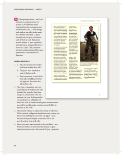
Figure 1: Left: fragment length distribution; Right: read start distribution
> bam0 <- rmShortInserts(K562.r1l1, isizeMin=100)
> distrs <- getDistrs(hg19DB,bam=bam0,readLength=75)
We visualize the fragment length distribution. The resulting plot is shown
in Figure 1, left panel. Notice there few fragments shorter than 140bp. Given
the reduced number of reads in our toy data the estimate is not accurate,
and hence we overlay a smoother estimate (blue line).
> plot(distrs, "fragLength")
We produce a histogram to inspect the read start distribution. The histogram reveals that reads are non-uniformly distributed along transcripts
(Figure 1, right panel). Rather, there is a bias towards the 3’ end.
> plot(distrs, "readSt")
As a final pre-processing step, we use the function procBam to divide each
read pair into a series of disjoint intervals. The intervals indicate genomic
regions that the read aligned to consecutively, i.e. with no gaps.
> pbam0 <- procBam(bam0)
> pbam0
procBam object created from non-stranded reads
Contains 43009 ranges corresponding to 17344 unique read pairs
> head(getReads(pbam0))
GRanges with 6 ranges and 3 metadata columns:
seqnames
ranges strand |
rid
XS
names
<Rle>
[1]
chr17
[2]
chr17
[3]
chr17
[4]
chr9
[5]
chr9
[6]
chrX
--seqlengths:
chr17 chr9
NA
NA
<IRanges>
[ 7124912,
7124986]
[ 7124986,
7125001]
[ 7125271,
7125329]
[ 94485006, 94485080]
[ 94485115, 94485189]
[133680161, 133680235]
chrX chr14 chr12 chr10
NA
NA
NA
NA
<Rle>
+
+
+
| <integer> <Rle> <integer>
|
1
*
0
|
2
*
0
|
2
*
0
|
1
*
1
|
2
*
1
|
1
*
2
chr3 chr16
NA
NA
chr1
NA
chr6
NA
chr7
NA
chr2
NA
chr8
NA
The resulting object pbam0 is a list with element pbam of type RangedData
and stranded indicating whether the RNA-seq experiment was stranded or
not.
5
Estimating expression for a set of known
variants
In order to obtain expression estimates, we first determine the exons visited
by each read, which we denominate the exon path, and count the number of
reads following the same exon path.
> pc <- pathCounts(pbam0, DB=hg19DB)
> pc
Non-stranded known pathCounts object with 21 islands and 15 non zero islands.
> head(pc@counts[[1]])
$`326`
NULL
$`463`
.17737-17738.
2
.17728.17729-17729.
1
.17731.17732-17732.
3
.17726-17726.
90
.17732.17733-17733.
.17726-17727. .17734-17735.17736.
1
1
3
.17726.17727-17727.
.17736-17736.
.17736-17737.
1
2
1
.17738.17741-17741. .17727.17728-17728.
.17737-17737.
1
1
1
.17728-17728.17729.
.17728-17729.
1
1
$`11211`
.129388.129389-129389.
.129389-129389. .129386.129387-129387.
1
48
1
.129382.129383-129383. .129381.129382-129382.
.129382-129382.
2
.129379.129380-129380.
3
1
.129383-129384.
2
1
.129381-129382.
1
$`14256`
.152698-152698.152699.
.152694-152694.152695.
1
2
.152691-152691.152692. .152684.152685-152685.152686.
2
1
.152730-152730. .152718.152719-152719.152720.
2
1
.152687.152688-152688.
.152694-152695.
1
1
.152712-152713. .152725.152726-152726.152727.
1
1
.152702-152703.
1
$`14325`
.154139-154140.
.154146-154146.
3
9
.154142.154143-154143.
.154142-154142.
2
1
.154141.154142-154142.
.154139-154139.154140.
2
1
.154138.154139-154139.
.154137.154138-154138.
3
5
.154144.154145-154146.
.154142-154143.
1
3
.154137-154138. .154143.154144-154144.154145.
2
1
.154143-154143.154144. .154142.154143-154143.154144.
1
1
.154142-154142.154143.
.154141-154141.154142.
1
3
.154140.154141-154141.154142. .154137.154138-154138.154139.
3
1
.154139.154140-154140.154141.
1
$`15370`
NULL
The output of pathCounts is a named integer vector counting exon paths.
The names follow the format ”.exon1.exon2-exon3.exon4.”, with dashes making the split between exons visited by left and right-end reads correspondingly. For instance, an element in pc named .1314.1315-1315.1316. indicates the number of reads for which the left end visited exons 1314 and
1315 and the right end visited exons 1315 and 1316. The precise genomic
coordinates of each exon are stored in the annotated genome.
The function calcExp uses the exon path counts, read start and fragment
length distributions and genome annotation to obtain RPKM expression estimates. Expression estimates are returned in an ExpressionSet object, with
RefSeq transcript identifiers as featureNames and the internal gene ids used
by hg19DB stored as feature data.
> eset <- calcExp(distrs=distrs, genomeDB=hg19DB, pc=pc, readLength=75, rpkm=FALSE)
> eset
ExpressionSet (storageMode: lockedEnvironment)
assayData: 52 features, 1 samples
element names: exprs
protocolData: none
phenoData: none
featureData
featureNames: NM_005158 NM_001168236 ... NM_005502 (52 total)
fvarLabels: transcript gene_id island_id explCnts
fvarMetadata: labelDescription
experimentData: use 'experimentData(object)'
Annotation:
> head(exprs(eset))
NM_005158
NM_001168236
NM_001136000
NM_001168239
NM_001136001
NM_007314
1
0.15246806
0.18206660
0.07945679
0.26803610
0.04616323
0.12214227
> head(fData(eset))
NM_005158
NM_001168236
NM_001136000
NM_001168239
NM_001136001
NM_007314
transcript gene_id island_id explCnts
NM_005158
27
463
110
NM_001168236
27
463
110
NM_001136000
27
463
110
NM_001168239
27
463
110
NM_001136001
27
463
110
NM_007314
27
463
110
When setting rpkm to FALSE, calExp returns relative expression estimates
for each isoform. That is, the proportion of transcripts originating from each
variant, so that the estimated expressions add up to 1 for each island. If
you would prefer relative expressions that add up to 1 within each gene you
can use function relexprByGene. When setting rpkm to TRUE, expression
estimates in reads per kilobase per million (RPKM) are returned instead.
> eset <- calcExp(distrs=distrs, genomeDB=hg19DB, pc=pc, readLength=75, rpkm=TRUE)
> head(exprs(eset))
NM_005158
NM_001168236
NM_001136000
NM_001168239
NM_001136001
NM_007314
1
5.674319
5.833150
5.048797
6.270137
6.198636
5.428798
Let π
ˆgi be the estimated relative expression for transcript i within gene
g, wgi the transcript
P width in base pairs, ng the number of reads overlapping
with gene g and
ng the total number of reads in the experiment. The
RPKM for transcript i within gene i is computed as
rgi = 109
6
π
ˆgi ng
P
wgi ng
(1)
Plots and querying an annotatedGenome
casper incorporates some functionality to plot splicing variants and estimated expression levels. While in general we recommend using dedicated
visualization software such as IGV [Robinson et al., 2011], we found useful
to have some plotting capabilities within the package.
We start by showing how to extract information from an annotatedGenome
object. Suppose we are interested in a gene with Entrez ID= 27. We can
obtain the known variants for that gene with the function transcripts, and
the chromosome with getChr. We can also find out the island identifier that
casper assigned to that gene (recall that casper merges multiple genes that
have some overlapping exons into a single gene island).
> tx <- transcripts(entrezid='27', genomeDB=hg19DB)
> tx
IRangesList of length 8
$NM_001168236
IRanges of length 13
start
end width names
[1] 179198376 179198819
444 17741
[2] 179100446 179100616
171 17738
[3] 179095512 179095807
296 17737
[4] 179090730 179091002
273 17736
[5] 179089325 179089409
85 17735
...
...
...
...
...
[9] 179081444 179081533
90 17731
[10]
[11]
[12]
[13]
179079417
179078343
179078034
179068462
179079590
179078576
179078342
179078033
174
234
309
9572
17729
17728
17727
17726
...
<7 more elements>
> getChr(entrezid='27',genomeDB=hg19DB)
[1] "chr1"
> islandid <- getIsland(entrezid='27',genomeDB=hg19DB)
> islandid
[1] "463"
> getChr(islandid=islandid,genomeDB=hg19DB)
[1] "chr1"
Once we know the islandid, we can plot the variants with genePlot. The
argument col can be set if one wishes to override the default rainbow colours.
> genePlot(islandid=islandid,genomeDB=hg19DB)
Figure 2 shows the resulting plot. The plot shows the identifiers for
all transcripts in the gene island, and exons are displayed as boxes. The
x-axis indicates the genomic position in bp. For instance, the last three
variants have a different transcription end site than the rest, indicated by
their last exon being different. Similarly, the first variant has an alternative
transcription start site.
It can also be useful to add the aligned reads and estimated expression
to the plot. This can be achieved by passing the optional arguments reads
(the object returned by procBam) and exp (the object returned by calcExp).
> genePlot(islandid=islandid,genomeDB=hg19DB,reads=pbam0,exp=eset)
Figure 3 shows the plot. Black segments correspond to pairs with short
insert size (i.e. where both ends are close to each other, by default up to
maxFragLength=500bp). They indicate the outer limits of the pair (i.e. leftmost position of the left read and right-most position of the right read).
Red/blue segments indicate pairs with long insert sizes. The red lines indicates the gapped alignments and the discontinuous blue lines simply fill in
the gaps, so that they are easier to visualize. By staring at this plot long
enough, one can make some intuitive guesses as to which variants may be
more expressed. For instance, many reads align to the left-most exon, which
NM_005158
NM_001136000
NM_001168239
NM_001136001
NM_007314
NM_001168237
NM_001168238
NM_001168236
179080000
179120000
179160000
179200000
Figure 2: Transcripts for gene with Entrez ID= 27
suggests that variant NM 00136001 is not highly expressed. Accordingly,
casper estimated expression for this variant is lowest. There are few reads
aligning to the exons to the right-end (which may be partially explained by
the presence of a 3’ bias). The last variant does not contain several of these
genes, and hence has the highest estimated expression. Of course, inspecting
the figure is simply meant to provide some intuition, to quantify alternative
splicing casper uses precise probability calculations.
References
Martin Morgan and Herv´e Pag`es. Rsamtools: Import aligned BAM file
format sequences into R / Bioconductor. URL http://bioconductor.
org/packages/release/bioc/html/Rsamtools.html. R package version
1.4.3.
J.T. Robinson, H. Thorvaldsd´ottir, W. Winckler, M. Guttman, E.S. Lander,
G. Getz, and J.P. Mesirov. Integrative genomics viewer. Nature Biotechnology, 29:24–26, 2011.
D. Rossell, C. Stephan-Otto Attolini, M. Kroiss, and A. St¨ocker.
Quantifying alternative splicing from paired-end RNA-sequencing
NM_001168236 (expr=5.833)
NM_001168238 (expr=5.037)
NM_001168237 (expr=4.893)
NM_007314 (expr=5.429)
NM_001136001 (expr=6.199)
NM_001168239 (expr=6.27)
NM_001136000 (expr=5.049)
NM_005158 (expr=5.674)
179080000
179120000
179160000
179200000
Figure 3: Transcripts for gene with Entrez ID= 27
data.
Annals of Applied Statistics, 8(1):309–330, 2014.
http://www.e-publications.org/ims/submission/AOAS/user/
submissionFile/13921?confirm=ede240bc.
URL
C. Trapnell, L. Pachter, and S.L. Salzberg. Tophat: discovering splice junctions with rna-seq. Bioinformatics, 25(9):1105–11, May 2009.


© Copyright 2026