1. No category

Supporting Information
Bacot-Davis et al. 10.1073/pnas.1411098111
SI Materials and Methods
LE Phosphorylation Assays. Recombinant GST-LE (EMCV) proteins and mutational derivatives T3A, T4A, T9A, T15A, Y27F,
Y32F, Y36F, Y41F, T47A, T47E, and Y41F/T47A were expressed
and purified as previously described (1–3). Each protein was
dialyzed into buffer [25 mM Hepes (pH 7.3), 150 mM KCl, and
2 mM DTT] and stored at −80 °C. Concentrations were determined
with BCA protein assay kits (Thermo Scientific). The cell-free
phosphorylation assays were essentially as previously described (4).
GST (85 pmol) or GST-LE (85.71 pmol) was incubated with buffer
alone, CK2 (10 U; New England Biolabs), or CK2 (10 U) plus Syk
(10.3 U; SignalChem) in the manufacturers’ reaction buffers supplemented with 5.0 μCi [γ-32P] ATP (3,000 Ci/mmol, 10 mCi/mL).
After incubation at 37 °C for 60 min, samples were loaded for SDS/
PAGE fractionation. To evaluate the Syk (only) reactions, the
proteins were pretreated with CK2 and (cold) ATP before the
addition of Syk and [γ-32P] ATP. The resolved gels were silver
stained and then exposed to phosphor screens for band visualization (GE Healthcare).
LM for NMR. Unlabeled GST-LM (Mengo) fusion protein was
expressed in E. coli as previously described (5). Bacterial cultures
contained 25 μM ZnCl2 for proper protein folding. The expressed
protein included a thrombin cleavage site for GST-tag removal.
[15N/13C]-LM0P was produced from BL-21 (DE3) cells transformed with pGST-LM at 16 °C in [15N/13C] M9 medium [42.3 mM
Na2HPO4, 22.0 mM KH2PO4, 8.5 mM NaCl, 18.3 mM 15NH4Cl,
2 mM MgSO4, 0.1 mM CaCl2, 0.2% 13C -D-glucose (wt/vol),
50 μg/mL kanamycin, pH 7.3] before induction with isopropylβ-D-thiogalactopyranoside (IPTG, 1 mM). Cells were collected at
an OD600 of 2.7–3.2. Harvest was on GSTrap FF columns, where
the GST tags were removed before elution by reaction with
thrombin protease as previously described (3). The affinity
chromatography was followed by gel filtration using a Sephacryl
S-100 column (GE Healthcare) and finally anion exchange with
a Mini Macro-Prep High Q cartridge (Bio-Rad). The protein was
concentrated using an Amicon Ultracentrifuge device (Millipore),
treated with 0.25 mM EDTA for 5 min at 25 °C and then refolded
by dialysis (2 L, 20 mM Hepes, pH 7.5, 100 mM KCl, 2 mM DTT,
0.25 mM ZnCl2, 12 h, 4 °C). The protein was then dialyzed twice
more into NMR buffer (20 mM Hepes, pH 7.5, 150 mM KCl, 2
mM MgCl2, 5 mM DTT, 0.04% NaN3, 12 h, 4 °C) before storage
at −80 °C. The molecular weight of [15N/13C]-LM0P was determined by matrix-assisted laser desorption ionization-MS
(MALDI-MS) using a Bruker BIFLEX III mass spectrometer.
Protein purity (>95%) was determined by SDS/PAGE followed
by silver stain. Care was taken at all steps to use NMR-grade,
metal-free reagents.
LM Phosphorylation. [15N/13C]-LM0P was purified by gel filtration,
concentrated, and then incubated with CK2 alone (10 U) or with
CK2 (10 U) followed by Syk (10.3 U) in a reaction buffer supplemented with 200 μM [31P]ATP. The buffers were as provided
by the manufacturers. Reactions were at 37 °C for 2.5 h. After
phosphorylation, [15N/13C]-LM(1P/2P) was dialyzed (10 mM BisTris propane, pH 7.4, 50 mM NaCl, and 2 mM DTT) and purified by anion exchange using a Mini Macro-Prep High Q cartridge (Bio-Rad) over a 20-column volume salt gradient (50–500
mM NaCl) to remove the kinases. The proteins were treated
with 0.25 mM EDTA for 5 min at 25 °C, refolded (as above),
dialyzed into NMR buffer (as above), and then stored at −80 °C.
Bacot-Davis et al. www.pnas.org/cgi/content/short/1411098111
Ran for NMR. Plasmids encoding Hexa-His-Xpress–tagged human
Ran GTPase (His-Xp-Ran) were a gift from Mary Dasso (National Institutes of Health, Bethesda, MD). Unlabeled protein was
expressed in BL21 cells as previously described (3). [15N/13C]
preparations were similar, except the cells were grown at 30 °C in
M9 medium as described for [15N/13C]-LM, with 50 μg/mL ampicillin instead of kanomycin. Initial protein purification steps
(labeled or unlabeled) were as previously described (3), using
a two-tier process of HisTrap HP (GE Healthcare) affinity chromatography followed by gel filtration using a Sephacryl S-100
column (GE Healthcare). If for use in NMR, the samples were
treated with EDTA (5 mM, 30 min, 25 °C) and dialyzed (2 h,
25 °C) into NMR buffer (2 L, 20 mM Hepes, pH 7.4, 100 mM KCl,
2 mM MgCl2, 2 mM DTT, and 0.04% NaN3), followed by a second
dialysis into fresh NMR buffer (overnight, 4 °C). Care was taken at
all steps to use NMR-grade, metal-free reagents. Ran prepared this
way (259 aa) retains the expression tag (43 aa) at the amino terminus of the full-length protein (216 aa). Recombinant GST-RCC1
(X. laevis) was purified as previously described (6) and then dialyzed
into NMR buffer.
NMR Determinations. NMR data were collected at 25 °C using
280-μL samples in a 5-mm Shigemi tube. The protein concentration for labeled (15N/13C) or unlabeled LM(0P/1P/2P) and Ran was
0.5 mM in the independent determinations. For Ran:LM0P complexes, each protein was at 0.5 mM (one labeled and one unlabeled), and the samples were supplemented with (unlabeled)
GST-RCC1 (1.4 nmol). The resolved spectra, including [1H-15N]
HSQC, [1H-13C] HSQC, HBHA(CO)NH, CBCA(CO)NH,
C(CO)NH, HC(CO)NH, HC(C)H-TOCSY, 3D 15N-NOESY
(tmix = 120 ms), and 3D 13C-NOESY (tmix = 120 ms) were collected
on a Bruker DRX-600 spectrometer equipped with an 1H, 13C, 15N,
31
P three-axis gradient cryogenic probe. Standard NMR terminology includes NOESY (nuclear Overhauser effect spectroscopy),
NHCABA (carbon alpha, carbon beta, amide spectroscopy),
CBCA(CO)NH (carbon beta, carbon alpha, carbonyl spectroscopy),
HSQC (heteronuclear single quantum coherence spectroscopy),
TOCSY (total correlated spectroscopy), CARA (computer-aided
resonance assignment).
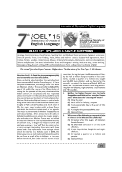
Data Processing. Fig. S1 shows a summary flowchart for all data
manipulations. The collected NMR data were processed using
NMR-Pipe software (7), followed by peak picking and spin-system
determination with CARA software (8). Cross-reference of 15NHSQC, 13C-HSQC, CBCACONH, HBHACONH, CCONH,
HCCONH, and HCCH-TOCSY spectra from uniformly labeled
15
N/13C proteins assigned backbone and side-chain atoms (e.g.,
Figs. S2 and S4). TALOS+/RAMA+ generated dihedral angle
constraint files (9) for input into CYANA (10) for structure calculations (Figs. S2 and S5B). The -ref comment alongside X-ray–
determined structures of Ran generated upper and lower references
for TALOS+ dihedral angle constraints in conjunction with chemical shifts assignments for NMR-resolved Ran (PDB ID code
2MMC) and Ran:(LM0P). Cross-correlation of 3D HCCH-TOCSY,
13
C-NOESY, and 15N-NOESY spectra, collected using a mixing
time set to 120 ms for all triple-labeled data acquisition, assigned
NOESY connectivity with CARA, SPARKY, CYANA, and CSRosetta (8, 10–14). Nonstandard amino acids and refinements
(Table S3) were finalized by using VMD-X-PLOR (15). The
quality of each generated structure was analyzed for restraint
and geometry violations using the Duke University MolProbity
web server (16, 17). All LM datasets (71 aa) recorded the (4 aa)
1 of 9
amino-terminal extensions. The Ran datasets omitted tagrelated peaks and numbered the protein (216 aa) according to
its native sequence. Additional information for many of these
technical processes is presented in the next sections.
H/15N couplings for solution-state
protein samples were measured using 1JNH modulation experiment,
as previously described (18), with the addition of an evolution
period during 2D 15N-HSQC data collections.
Residual Dipolar Coupling.
1
NMR-PIPE NOESY Processing. The command lines used to process
15
13
N/ C-NOESY spectra following data collected on a 600MHz Bruker spectrometer are provided in Dataset S1.
Dihedral Angle Constraints. Residue atoms were manually assigned
using CARA (8). CARA wrote *.tab files for input into TALOS+/
RAMA+, which generated de novo *.aco dihedral angular constraints and secondary structure element files. Peak lists and peak
tables were imported from CARA into SPARKY (11) for figure
visualization and assignment verification with PINE-SPARKY (19).
Automatic CYANA NOESY Assignments with CS-Rosetta Convergence.
Structure calculations were conducted by running CYANA 3.0
(e-NMR) with peak intensities from three NOESY spectra: TALOS+
dihedral angle constraints, residual decoupling restraints, and
initial, manually assigned NOE restraints as input files (10).
After several runs using TALOS+-derived dihedral angle constraints and increasingly convergent high-quality CS-Rosetta and
CYANA-derived NOE restraints, final automated NOESY assignments were generated in CYANA with the seeding NOEs.
Blind CS-Rosetta structure determination was also conducted
1. Porter FW, Bochkov YA, Albee AJ, Wiese C, Palmenberg AC (2006) A picornavirus
protein interacts with Ran-GTPase and disrupts nucleocytoplasmic transport. Proc Natl
Acad Sci USA 103(33):12417–12422.
2. Porter FW, Palmenberg AC (2009) Leader-induced phosphorylation of nucleoporins
correlates with nuclear trafficking inhibition by cardioviruses. J Virol 83(4):1941–1951.
3. Bacot-Davis VR, Palmenberg AC (2013) Encephalomyocarditis virus Leader protein hinge
domain is responsible for interactions with Ran GTPase. Virology 443(1):177–185.
4. Basta HA, Bacot-Davis VR, Ciomperlik JJ, Palmenberg AC (2014) Encephalomyocarditis
virus leader is phosphorylated by CK2 and syk as a requirement for subsequent
phosphorylation of cellular nucleoporins. J Virol 88(4):2219–2226.
5. Cornilescu CC, Porter FW, Zhao KQ, Palmenberg AC, Markley JL (2008) NMR structure
of the mengovirus Leader protein zinc-finger domain. FEBS Lett 582(6):896–900.
6. Nemergut ME, Macara IG (2000) Nuclear import of the ran exchange factor, RCC1, is
mediated by at least two distinct mechanisms. J Cell Biol 149(4):835–850.
7. Delaglio F, et al. (1995) NMRPipe: A multidimensional spectral processing system
based on UNIX pipes. J Biomol NMR 6(3):277–293.
8. Keller RLJ (2004) The Computer Aided Resonance Assignment Tutorial (Cantina Verlag, Germany).
9. Shen Y, Delaglio F, Cornilescu G, Bax A (2009) TALOS+: A hybrid method for predicting protein backbone torsion angles from NMR chemical shifts. J Biomol NMR
44(4):213–223.
10. Güntert P (2004) Automated NMR structure calculation with CYANA. Methods Mol
Biol 278:353–378.
11. Goddard TD, Kneller DG (2008) SPARKY 3. (University of California, San Francisco).
12. Bradley P, Misura KMS, Baker D (2005) Toward high-resolution de novo structure
prediction for small proteins. Science 309(5742):1868–1871.
13. Shen Y, et al. (2008) Consistent blind protein structure generation from NMR chemical
shift data. Proc Natl Acad Sci USA 105(12):4685–4690.
Bacot-Davis et al. www.pnas.org/cgi/content/short/1411098111
with final CYANA-derived dihedral angle and NOE constraint
files (14). CS-Rosetta models were similar to CYANA-determined
structures. For the LM structures, the 10 final CYANA-generated
coordinate sets (10) were too dynamic for PDB deposition, so in
each case, the low energy model 1 was further examined with the
Xplor-NIH package NAMD (15) energy minimization and collective variable analysis (PLUMED) to calculate the final, refined
10 states that were compatible with and deposited at PDB.
Structure Generation Using CYANA. TALOS+ *.aco torsion angle
constraint files, CYANA-derived *.upl residual dipolar coupling,
distance restraint files, and final assigned NOESY peak lists
were used as input into CYANA to calculate 50 structures to
output the 10 final low-energy states. Combinations of random
restraints were used to improve structure qualities as above
and as previously detailed (14). PRO-CHECK and AQUA
through ADIT-NMR were used to validate the final 10 NMRdetermined PDB-deposited structures (20).
Docking and Bioinformatics. TALOS+ algorithms (7) were used to
define α and β motifs within the determined structures (Fig. S5).
The lowest energy NMR states for LM0P and Ran, as determined
from the docked complexes, were submitted to HADDOCK via
the public web portal (21). No constraints were specified. Docking
interfaces for the lowest energy complex were evaluated online
using PDBePISA resources (www.ebi.ac.uk/pdbe/pisa/) and the
PIC (22). RMSDs for comparative states or pairwise structures
used the “align” function of PyMol (23), specifying only the
backbone c+n+ca+o atoms (Table S4). Structure display was
by PyMol or Chimera (24).
14. Lange OF, et al. (2012) Determination of solution structures of proteins up to 40 kDa
using CS-Rosetta with sparse NMR data from deuterated samples. Proc Natl Acad Sci
USA 109(27):10873–10878.
15. Schwieters CD, Clore GM (2001) The VMD-XPLOR visualization package for NMR
structure refinement. J Magn Reson 149(2):239–244.
16. Davis IW, et al. (2007) MolProbity: All-atom contacts and structure validation for
proteins and nucleic acids. Nucleic Acids Res 35(web server issue):W375-83.
17. Chen VB, et al. (2010) MolProbity: All-atom structure validation for macromolecular
crystallography. Acta Crystallogr D Biol Crystallogr 66(Pt 1):12–21.
18. Tjandra N, Grzesiek S, Bax A (1996) Magnetic fields dependence of nitrogen-proton J
splittings in 15N-enriched human ubiquitin resulting from relaxation interference and
residual dipolar coupling. J Am Chem Soc 118(26):6264–6272.
19. Lee W, Westler WM, Bahrami A, Eghbalnia HR, Markley JL (2009) PINE-SPARKY:
Graphical interface for evaluating automated probabilistic peak assignments in
protein NMR spectroscopy. Bioinformatics 25(16):2085–2087.
20. Laskowski RA, Rullmannn JA, MacArthur MW, Kaptein R, Thornton JM (1996) AQUA
and PROCHECK-NMR: {Programs for checking the quality of protein structures solved
by NMR. J Biomol NMR 8(4):477–486.
21. de Vries SJ, van Dijk M, Bonvin AMJJ (2010) The HADDOCK web server for data-driven
biomolecular docking. Nat Protoc 5(5):883–897.
22. Tina KG, Bhadra R, Srinivasan N (2007) PIC: Protein Interactions Calculator. Nucleic
Acids Res 35(web server issue):W473-6.
23. Anonymous (2008) The PyMOL Molecular Graphics System (Schrödinger, LLC), Version
1.1r.1.
24. Pettersen EF, et al. (2004) UCSF Chimera—a visualization system for exploratory research and analysis. J Comput Chem 25(13):1605–1612.
2 of 9
Experimental data
collection
Data:
15N-HSQC
13C-HSQC
CBCACONH
HBHACONH
CCONH
HCCONH
HCCH-TOCSY
15N-NOESY
13C-NOESY
Final
ensembles
Xplor-NIH
refinement &
PROCHECK
validation
Manual backbone
and side-chain resonance
assignments
10 ensembles
Manual NOEs
CYANA
Improve
assignments
CYANA NOEs
(final.upl)
NO
CS-ROSETTA
structures
converge?
YES
Fig. S1. Work flow of NMR structure determinations. Restraints files were generated from chemical shift assignments using TALOS+/RAMA+, CYANA, and CSRosetta suites for each determination, as indicated.
Bacot-Davis et al. www.pnas.org/cgi/content/short/1411098111
3 of 9
LM0P 15N-HSQC
A.
10
C.
9
8
7
LM0P
TOCSY/NOESY Strip plot
G53N-H
ω1 -15N (ppm)
110
D41N- E48N-H
H
E65N- H
E21NT7NS27NT51NT70N-H
T8N-
115
120
H16N-H
C26N-H
125
C14N-H
110
G34N-H
S17N-H
L49N-H
T19N-
115
E22N-H
K25NH
Q30N-H
Q11ND61NN33N-HL29NF35NH
Y31NM5N-HM18NH
E54N-A15NHM64ND56N-H
E42NV57NI13NH
D63NHH K39NY40NE47N-H
E10NE69NE43N-HHD52NH E12NY36NV66NF20N- R32NH M9NH H
L38NL62N-H
T3N- HW44NHH
C23NS2NL37ND55NH A28N-H
V67NHY45N-H
L50NF68N- H
D59N-H
F58N-
120
125
Q71N-H
A4N-H
A6N-H
130
130
10
9
7
8
ω2- 1H (ppm)
LM0P 15N-HSQC
B.
110
ω1 -15N (ppm)
111
112
8.4
8.2
8.0
111
D41N-H
E48N-H
E65N-H
112
E21N-H
T7N-H
S27N-H
113
7.8
110
113
114
T51N-H
114
115
T70N-H
T8N-H
115
116
117
116
8.4
8.2
ω2- 1H (ppm)
8.0
D59
S27
T7
L62
E21
117
7.8
Fig. S2. Nuclei assignments for LM0P. (A) 2D 15N-HSQC assignments were used to determine 15N-NOESY J-coupling connectivity. All assigned peaks are labeled.
(B) Section of resonances of the 2D 15N-HSQC of LM0P, from A, magnified for clarity. (C) TOCSY-NOESY connectivity strips for LM0P residues; D59, S27, T7, L62,
and E21 are shown as examples.
Bacot-Davis et al. www.pnas.org/cgi/content/short/1411098111
4 of 9
LM0P/1P/2P:(Ran)15N-HSQC
14
12
A.
ω1 -15N (ppm)
100
LM0P
LM1P
LM2P
LM0P:(Ran)
8
6
100
T19N-H
110
120
10
E42N-H
H16N-H
120
C26N-H
C14N-H
D52N-H
A4N-H
130
T3N-H
140
B.
S2N-H
14
12
LM0P:(Ran)
Ramachandran plot quality
Resolution
(angstroms)
C.
110
L49N-H
V67N-H
10
ω2- 1H (ppm)
LM0P:(Ran)
8
D.
A4N-H
130
E
6
140
LM0P:(Ran)
H-bond energy
Dihedral angle G-factor
Resolution
(angstroms)
Resolution
(angstroms)
Fig. S3. LM(0P/1P/2P) stereochemical parameters. (A) 2D 15N-HSQC of LM0P, LM1P, LM2P, and LM0P:(Ran). To avoid obscuring visualization of the superimposed
datasets, only a few peaks are shown as labeled. A fully annotated version of this image is available from the authors. (B) A 1.8-Å resolution Ramachandran
plot quality. (C) Hydrogen bond energy SD of 0.6 compared with a typical value of 1.3. (D) Dihedral angle G-factor of 0.2 is within the favored region of
dihedral angle conformations. For B–D, white box is current structure.
Bacot-Davis et al. www.pnas.org/cgi/content/short/1411098111
5 of 9
Ran:(LM0P) 15N-HSQC
12
10
8
A.
105
ω1 -15N (ppm)
110
115
120
125
130
135
-
V106N-
Q239NK81N-Y82NR183NE-HE
S178N- A235NA247NA126NV88N- L74N-L205NQ188NE2-HE21
T250N- L56NM44N- T97NQ51N- N143NC163NY141N- R119NH1-HH11
H R172NH2-HH22
K185N- T67NK71NF69NE113NF115N242NE2-HE2
G111NR99NH2-HH21
I169N-R119NK114N- T85N- G116NK177NV94NE245NR183NH1-HH11
V161NL236NQ239NE2-HE21
H
D108NL207NY198NI131NC128NF104N- H148NG62NK166NZ-HZ
A237NM222NK66NL225NM232NR209N-D254N- N146NY190NHI160N-F200N-R183NH2-HH21
H148ND1-HD1
I179NR138NE-HE
F95N-A46N- D243N- N197ND2-HD21
N165NH91ND1-HD1
R149ND258N- H R119NE-HE
G60N-G100NV231N- Q248NE2-HE22
I102NH91N- K55NN186ND2-HD22
V246NG63NH242ND1-HD1 H182ND1-HD1 E89NE255NA45N- N98NQ125NE2-HE21
W206NE1-HE1
W107NE1-HE1
W147NE1-HE1
A176NS196NF219NH73NE2-HE2
H91NE2-HE2
K175N- V174N-
12
B.
105
Ran:(LM0P)
TOCSY/NOESY Strip plot
110
115
120
125
130
135
6
10
8
ω2- 1H (ppm)
Ran:(LM0P) 15N-HSQC
10.0
9.5
9.0
8.5
106
ω1 -15N (ppm)
C.
6
108
108
R183NE-HE
110 K175N-H V174N-H
E113N-H
V
116
10.0
6110
K
A247N-H
V88N-H
T68N-H
T14 112
M44N-H
R138
C163NK185N-H L259N-H
114
T67N-H
112
114
8.0
V106N-H 106
K114N-H
9.0
H 8.5
ω2- 1H (ppm)
9.5
116
H
8.0
K28
R29
H30
15
Fig. S4. Nuclei assignments for Ran:(LM0P). (A) 2D N-HSQC assignments of Ran, titrated with LM0P, were used to determine 15N-NOESY J-coupling connectivity. To avoid obscuring the complete visualization of most peaks, some assigned labels have been removed. A fully annotated version of this image is
available from the authors. (B) A section of Ran:(LM0P) 2D 15N-HSQC residue resonances from A is magnified for clarity. (C) TOCSY-NOESY connectivity strips for
Ran:(LM0P) residues K28, R29, and H30 are shown as examples.
Bacot-Davis et al. www.pnas.org/cgi/content/short/1411098111
6 of 9
A. TALOS+ Predictions:
alpha,
B. Constraints:
beta
LM0P
10-1 -
β
40-
α
20-
β
40-
α
20-
0-
LM1P
10-1 -
0-
LM2P
40-
1-
β
0-
α
-1 -
LM0P:(Ran)
1-
β
0-
α
-1 -
|
0
Chi,
Phi-Psi
LM1P
LM2P
20040-
LM0P:(Ran)
200-
|
10
|
20
|
|
|
30
40
50
LM Sequence (aa)
|
60
|
67
Ran:(LM0P)
0-1 -
|
20
|
0
60-
1-
|
0
NOESY,
LM0P
|
40
|
60
β
40-
α
20-
|
|
|
|
|
|
|
|
80 100 120 140 160 180 200 216
Ran Sequence (aa)
|
10
|
20
|
|
|
30
40
50
LM Sequence (aa)
|
60
|
70
Ran:(LM0P)
0-
|
0
|
20
|
40
|
60
|
|
|
|
80 100 120 140
Ran Sequence (aa)
|
160
|
180
|
200
|
216
Fig. S5. (A) TALOS+ refinement. TALOS+/RAMA+ used the random coil index (RCI) method and Artificial Neural Network (ANN) to predict the secondary
structures for Ran residues. Positive values (aqua) represent β-sheet structure predictions, negative values (red) represent α-helix structure predictions, and
values of zero represent random coil conformations. Chemical shift-derived values are plotted for LM0P, LM1P, LM2P, LM0P:(Ran), and Ran:(LM0P) according to
each sequence. (B) As per the workflow chart in Fig. S1, constraints for each structure were generated from chemical shift assignments using TALOS+/RAMA+,
CYANA, and CS-Rosetta suites. Observed NOESY (green), Chi (red), and Phi-Psi (blue) constraints are plotted as stacked bars for each residue.
Bacot-Davis et al. www.pnas.org/cgi/content/short/1411098111
7 of 9
A.
LM0P:Ran stereo pair
B. LM0P
C. LM1P
D.
E. L 0P:(Ran)
M
LM2P
CYANA ensembles,10 states before VMD-X-PLORE refinement
Fig. S6. (A) Stereo images of Ran:LM0P complex. Illustration from Fig. 4C is reproduced as a stereo pair. (B–E) The 10 low-energy CYANA-generated coordinate
files for each LM determination are shown superimposed according to the common zinc finger motifs, using the PyMol align function. These figures illustrate
the original sampling of dynamic ensembles. The initial states were then further culled into more a refined, low-energy, related series of PDB-acceptable
ensembles (i.e., Figs. 2 and 4), as described in SI Materials and Methods.
Table S1. GST-LE phosphorylation sites
Kinase†
Substrate*
GST
GST-LE
GST-LE
GST-LE
GST-LE
GST-LE
GST-LE
GST-LE
GST-LE
GST-LE
GST-LE
GST-LE
GST-LE
T3A
T4A
T9A
T15A
Y27F
Y32F
Y36F
Y41F
T47A
T47E
Y41F/T47A
CK2
Syk‡
CK2+Syk
−
+
+
+
+
+
+
+
+
+
−
−
−
−
+
+
+
+
+
+
+
+
−
−
+
−
−
+
+
+
+
+
+
+
+
+
−
+
−
*Recombinant GST-LE and mutant derivatives were prepared as in Materials
and Methods.
†
Reactions with these enzymes and [32P]ATP gave strongly labeled proteins
(+) as in or failed to label (−).
‡
Reactions recording [32P]ATP incorporation with Syk (only) were preceded
by reactions with CK2 in the presence of unlabeled ATP.
Bacot-Davis et al. www.pnas.org/cgi/content/short/1411098111
8 of 9
Table S2. Ran NOESY distance restraints
Number of NOESY peaks
Number of CYANA restraints
Long range*
Picked Manual CYANA Restraints SUP† = 1 SUP† < 1 Violated distant restraints Violated angle restraints
Target
LM0P
LM1P
LM2P
LM0P:(Ran)
Ran:(LM0P)
885
580
804
1059
5636
11
8
0
1
192
874
572
804
1058
5444
256
129
353
397
600
18
14
11
11
82
19
15
11
11
53
0
0
0
0
0
0
1
0
0
5
Summary of NOESY cross-peaks used in LM0P and Ran:(LM0P) assignments with CYANA. Columns indicate cross-peaks for each
respective group. CYANA semiautomated peak picking followed initial manual assignments. CYANA-generated NOE distance restraint
reliabilities fell from 0 to 1. Combinations of random restraints were used to improve structure qualities as previously detailed (14).
*Long-range restraints ji-jj ≥ 5.
†
SUP, reliability of constraints as assigned by CYANA from 0 to 1.
Table S3. Structure quality
Crystallography
equivalent resolution
H-bond energy (Å)
Dihedral angles
G-factor (Å)
Ramachandran
plot quality (Å)
H-bond mean
parameter
1.5
1.7
1.1
1.2
1.5
0.2/1.0
0.1/1.0
0.1/1.0
0.2/1.0
0.4/1.0
1.8
2.3
2.2
1.8
1.0
0.7
0.7
0.6
0.6
0.7
LM0P
LM1P
LM2P
LM0P:(Ran)
Ran:(LM0P)
PROCHECK/AQUA suites (20) through ADIT-NMR, assessed each structure quality as a final validation before
PDB and BMRB deposition.
Table S4. Ran:(LM0P) relative to crystallographic determinations
Ran PDB
Å RMSD vs. Ran:(LM0P)-state 1
1I2M
1BYU
3GJ0
1K5G
3GJX
3EA5
2BKU
1RRP
Ran:(LM0P) States 2–10
Average
Variance
Bound GNP
Length
All 1–216
Core 8–176
COOH 177–216
P-loop 16–25
Switch 1 32–45
Switch 2 66–79
0
GDP
GDP
GTP
GTP
GTP
GTP
GTP
8–176
9–177
1–207
8–213
9–179
6–179
9–177
8–211
3.9
12.7
12.6
4.6
1.6
1.9
1.7
4.9
3.9
4.0
4.0
0.4
1.6
1.8
1.7
1.1
—
—
7.1
3.6
—
—
4.3
0.3
0.2
0.2
0.3
0.2
0.2
0.2
0.3
3.5
4.1
4.2
0.3
0.3
0.4
0.5
0.6
3.2
3.2
3.2
0.3
3.4
3.4
3.4
2.3
0
—
1–216
—
4.5
0.4
0.2
0.0
4.9
1.2
0.1
0.0
0.2
0.0
0.1
0.0
Backbone atoms of Ran (n+ca+c+o), within the indicated PDB files, were compared with Ran:(LM0P)-state-1 using the PyMOL align function over the
indicated residues. Similar alignments assessed variance among all pairwise Ran:(LM0P) state 1–10 coordinates. RMSD values rounded to 0.1 Å. Length is the
resolved residues within each file.
Other Supporting Information Files
Dataset S1 (DOCX)
Bacot-Davis et al. www.pnas.org/cgi/content/short/1411098111
9 of 9