
M B H IOPHYSICS
HANDBOOK OF MODERN BIOPHYSICS Series Editor Thomas Jue University of California Davis Davis, California For other titles published in this series, go to www.springer.com/series/7845 Thomas Jue Editor Fundamental Concepts in Biophysics Volume 1 Editor Thomas Jue, Ph.D. Department of Biochemistry and Molecular Medicine University of California Davis One Shields Avenue Davis, CA 95616, USA [email protected] ISBN: 978-1-58829-973-4 e-ISBN: 978-1-59745-397-4 DOI: 10.1007/978-1-59745-397-4 Library of Congress Control Number: 2009921740 © Humana Press, a part of Springer Science+Business Media, LLC 2009 All rights reserved. This work may not be translated or copied in whole or in part without the written permission of the publisher (Humana Press, c/o Springer Science+Business Media, LLC, 233 Spring Street, New York, NY 10013, USA), except for brief excerpts in connection with reviews or scholarly analysis. Use in connection with any form of information storage and retrieval, electronic adaptation, computer software, or by similar or dissimilar methodology now known or hereafter developed is forbidden. The use in this publication of trade names, trademarks, service marks, and similar terms, even if they are not identified as such, is not to be taken as an expression of opinion as to whether or not they are subject to proprietary rights. While the advice and information in this book are believed to be true and accurate at the date of going to press, neither the authors nor the editors nor the publisher can accept any legal responsibility for any errors or omissions that may be made. The publisher makes no warranty, express or implied, with respect to the material contained herein. Cover Illustration: Patch-Clamp fluorometry of an excised inside-out membrane patch. Printed on acid-free paper springer.com/humana PREFACE Over the past several years, I have organized and taught a core course in Modern Biophysics Techniques at the University of California Davis. Graduate students in biophysics, chemistry, physics, and engineering enroll in the class to survey the physical techniques that scientists use to study biology. Introducing the diverse and complex field of biophysics in an academically rigorous but interesting way poses daunting challenges. Indeed, the course has undergone many transformations and has tried on many styles: seminar/journal club, lecture/lab, and just plain didactic lecture formats. These, however, have achieved limited success, because they either assume a strong mathematics/physical-science background or reduce the physical science to a pedestrian level of knowledge, or demand that students trudge along with the expert researchers. None have attracted the interest of biology, physiology, or medical students, who must search for the biological meaning within biophysics. One major obstacle to developing an attractive but scholarly course centers on the balance between formalism and perspective. Each biophysics technique requires a mastery of a challenging set of physical-science/mathematics formalism. Yet even with mastery the reader may still not gain a biomedical perspective. How will these biophysical techniques help clarify the complex issues in biology? Moreover, how will the course deal with biomedical students’ reluctance to overcome the imposing physical-science/mathematical formalism in order to gain new perspectives on biology? These considerations have given rise to the series Handbook of Modern Biophysics. The books in this series will bring current biophysics topics into focus and expand as the field of biophysics expands, so that biology and physical-science students or researchers can learn fundamental concepts and apply new biophysics techniques to address biomedical questions. However, the chapter structure will recognize the demand for explicating the conceptual framework of the underlying physics formalism and for casting perspectives on the biomedical applications. Each chapter will have a bipartite structure: the first part establishes the fundamental physics concepts and describes the instrumentation or technique, while the second illustrates current applications in addressing complex questions in biology. With the addition of problem sets, further study, and references, the interested reader will be able to further explore the ideas presented. In the first volume, Fundamental Concepts in Biophysics, the authors lay down a foundation for biophysics study. Rajiv Singh opens the book by pointing to the central importance of “Mathematical Methods in Biophysics.” William Fink follows with a discussion on “Quantum Mechanics Basic to Biophysical Methods.” Together, these two chapters establish some of the principles of mathematical physics underlying many biophysics techniques. Because computer modeling forms an intricate part of biophysics research, Subhadip Raychaudhuri and colleagues introduce the use of computer modeling in “Computational Modeling of Receptor–Ligand Binding and Cellular Signaling Processes.” Yin Yeh and coworkers bring to the reader’s attention the physical basis underlying the common use of fluorescence spectroscopy in biomedical research in their chapter “Fluorescence Spectroscopy.” Electrophysiologists have also applied biophysics techniques in the study of membrane proteins, and Tsung-Yu Chen et al. explore v vi PREFACE stochastic processes of ion transport in their “Electrophysiological Measurements of Membrane Proteins.” Michael Saxton takes up a key biophysics question about particle distribution and behavior in systems with spatial or temporal inhomogeneity in his chapter “Single-Particle Tracking.” Finally, in “NMR Measurement of Biomolecule Diffusion,” Thomas Jue explains how magnetic resonance techniques can map biomolecule diffusion in the cell to a theory of respiratory control . This book thus launches the Handbook of Modern Biophysics series and sets up for the reader some of the fundamental concepts underpinning the biophysics issues to be presented in future volumes. Thomas Jue Biochemistry & Molecular Medicine University of California Davis CONTENTS 1 Mathematical Methods in Biophysics Rajiv R.P. Singh 1.1. 1.2. 1.3. 1.4. 1.5. 1.6. 1.7. 1.8. 1.9. 2 Functions of One Variable and Ordinary Differential Equations ........................................ Functions of Several Variables: Diffusion Equation in One Dimension ............................. Random Walks and Diffusion ............................................................................................. Random Variables, Probability Distribution, Mean, and Variance ..................................... Diffusion Equation in Three Dimensions ............................................................................ Complex Numbers, Complex Variables, and Schrödinger's Equation ................................ Solving Linear Homogeneous Differential Equations......................................................... Fourier Transforms.............................................................................................................. Nonlinear Equations: Patterns, Switches and Oscillators .................................................... 1 2 4 7 8 9 10 13 14 Quantum Mechanics Basic to Biophysical Methods William Fink 2.1. 2.2. 2.3. 2.4. 2.5. 2.6. 2.7. 3 Quantum Mechanics Postulates........................................................................................... One-Dimensional Problems................................................................................................. The Harmonic Oscillator ..................................................................................................... The Hydrogen Atom............................................................................................................ Approximate Methods ......................................................................................................... Many Electron Atoms and Molecules ................................................................................. The Interaction of Matter and Light .................................................................................... 17 23 27 30 33 36 38 Computational Modeling of Receptor–Ligand Binding and Cellular Signaling Processes Subhadip Raychaudhuri, Philippos Tsourkas, and Eric Willgohs 3.1. 3.2. 3.3. 3.4. 3.5. 3.6. Introduction ......................................................................................................................... Differential Equation-Based Mean-Field Modeling ............................................................ Application: Clustering of Receptor–Ligand Complexes.................................................... Modeling Membrane Deformation as a Result of Receptor–Ligand Binding ................................................................................................... Limitations of Mean-Field Differential Equation-Based Modeling .................................... Master Equation: Calculating the Time Evolution of a Chemically Reacting System .................................................................................................................. 41 42 45 46 47 47 vii viii CONTENTS 3.7. 3.8. 3.9. 3.10. 3.11. 3.12. 3.13. 3.14. 3.15. 3.16. 3.17. 4 Stochastic Simulation Algorithm (SSA) of Gillespie .......................................................... Application of the Stochastic Simulation Algorithm (SSA)................................................ Free Energy-Based Metropolis Monte Carlo Simulation .................................................... Application of Metropolis Monte Carlo Algorithm............................................................. Stochastic Simulation Algorithm with Reaction and Diffusion: Probabilistic Rate Constant–Based Method ........................................................................ Mapping Probabilistic and Physical Parameters.................................................................. Modeling Binding between Multivalent Receptors and Ligands......................................... Multivalent Receptor–Ligand Binding and Multimolecule Signaling Complex Formation............................................................................................................. Application of Stochastic Simulation Algorithm with Reaction and Diffusion........................................................................................................ Choosing the Most Efficient Simulation Method ................................................................ Summary ............................................................................................................................. 48 49 49 50 51 51 53 54 55 55 56 Fluorescence Spectroscopy Yin Yeh, Samantha Fore, and Huawen Wu 4.1. 4.2. 4.3. 4.4. 4.5. 4.6. 5 Introduction ......................................................................................................................... Fundamental Process of Fluorescence................................................................................. Fluorescence Microscopy.................................................................................................... Types of Biological Fluorophores ....................................................................................... Application of Fluorescence in Biophysical Research ........................................................ Dynamic Processes Probed by Fluorescence....................................................................... 63 64 71 76 86 96 Electrophysiological Measurements of Membrane Proteins Tsung-Yu Chen, Yu-Fung Lin, and Jie Zheng 5.1. 5.2. 5.3. 5.4. 5.5. 5.6. 5.7. 5.8. 5.9. Membrane Bioelectricity ..................................................................................................... Electrochemical Driving Force............................................................................................ Voltage Clamp versus Current Clamp................................................................................. Principles of Silver Chloride Electrodes.............................................................................. Capacitive Current and Ionic Current.................................................................................. Gating and Permeation Functions of Ion Channels ............................................................. Two-Electrode Voltage Clamp for Xenopus Oocyte Recordings ........................................ Patch-Clamp Recordings ..................................................................................................... Patch-Clamp Fluorometry ................................................................................................... 111 112 114 115 115 116 118 122 137 HANDBOOK OF MODERN BIOPHYSICS, VOLUME 1 6 ix Single-Particle Tracking Michael J. Saxton 6.1. 6.2. 6.3. 6.4. 6.5. 6.6. 6.7. 6.8. 6.9. 6.10. 6.11. Introduction ......................................................................................................................... The Broader Field................................................................................................................ Labeling the Dots ................................................................................................................ Locating the Dots ................................................................................................................ Connecting the Dots ............................................................................................................ Interpreting the Dots: Types of Motion ............................................................................... Is It Really a Single Particle? .............................................................................................. Enhancing z-Resolution....................................................................................................... Can a Single Fluorophore Be Seen in a Cell?...................................................................... Colocalization...................................................................................................................... Example: Motion in the Plasma Membrane Is More Complicated than is Often Assumed ................................................................................... 6.12. Example: From DNA to Protein.......................................................................................... 6.13. Example: Infection of a Cell by a Virus .............................................................................. 7 147 148 150 153 158 158 163 164 165 165 167 168 169 NMR Measurement of Biomolecule Diffusion Thomas Jue 7.1. 7.2. 7.3. 7.4. 7.5. 7.6. 7.7. 7.8. 7.9. 7.10. 7.11. 7.12. 7.13. 7.14. 7.15. 7.16. 7.17. 7.18. Introduction ......................................................................................................................... Relaxation and Field Gradient Measurement of Diffusion.................................................. Frequency Encoding of Spatial Position with Field Gradient ............................................. Phase Encoding by the Field Gradient................................................................................. Diffusion and Pulsed Field Gradient Signal Intensity ......................................................... Fick’s Laws of Diffusion..................................................................................................... Biomolecule Diffusion in the Cell....................................................................................... Stimulated Echo and Biomolecule Diffusion in the Cell..................................................... Myoglobin Function in the Cell........................................................................................... Perfused Heart Model.......................................................................................................... O2 Diffusion in Muscle Cell ................................................................................................ Translational Diffusion of Mb in Vitro ............................................................................... Translational Diffusion of Mb In Vivo................................................................................ Mb Contribution to O2 transport in Vivo ............................................................................. Mb-Facilitated Diffusion and Myocardial Function............................................................ Mb-Facilitated Diffusion and Skeletal Muscle Function..................................................... Cytoplasmic Properties and Architecture ............................................................................ Summary ............................................................................................................................. 181 182 183 184 187 188 189 190 190 191 192 193 193 193 195 195 196 196 Problem Solutions...................................................................................................... 201 Index............................................................................................................................ 233 CONTRIBUTORS Tsung-Yu Chen (chap. 5) Center for Neuroscience Department of Neurology University of California Davis 1544 Newton Court Davis, CA 95618 USA [email protected] Michael J. Saxton (chap. 6) Department of Biochemistry & Molecular Medicine University of California Davis One Shields Avenue Davis, CA 95616 USA [email protected] William H. Fink (chap. 2) Department of Chemistry University of California Davis One Shields Avenue Davis, CA 95616 USA [email protected] Rajiv R.P. Singh (chap. 1) Department of Physics University of California Davis One Shields Avenue Davis, CA 95616 USA [email protected] Samantha Fore (chap. 4) Center for Biophotonics Science and Technology University of California, Davis 2700 Stockton Blvd., Suite 1400 Sacramento, CA 95817 USA [email protected] Philippos Tsourkas (chap. 3) Department of Biomedical Engineering University of California Davis One Shields Avenue Davis, CA 95616 USA Thomas Jue (chap. 7) Department of Biochemistry & Molecular Medicine One Shields Avenue University of California Davis Davis, CA 95616 USA [email protected] Yu-Fung Lin (chap. 5) Departments of Anesthesiology, & Physiology and Membrane Biology University of California Davis One Shields Avenue Davis, CA 95616 USA Subhadip Raychaudhuri (chap. 3) Department of Biomedical Engineering University of California Davis One Shields Avenue Davis, CA 95616 USA [email protected] Eric Willgohs (chap. 3) Department of Biomedical Engineering University of California Davis One Shields Avenue Davis, CA 95616 USA Huawen Wu (chap. 4) Department of Applied Science University of California, Davis One Shields Avenue Davis, CA 95616 USA [email protected] Yin Yeh (chap. 4) Department of Applied Science University of California, Davis One Shields Avenue Davis, CA 95616 USA [email protected] Jie Zheng (chap. 5) Department of Physiology & Membrane Biology University of California Davis One Shields Avenue Davis, CA 95616 USA xi 1 MATHEMATICAL METHODS IN BIOPHYSICS Rajiv R.P. Singh Department of Physics, University of California Davis 1.1. FUNCTIONS OF ONE VARIABLE AND ORDINARY DIFFERENTIAL EQUATIONS Quantitative relationships between different variables are represented as mathematical functions. For example, the number of proteins of a certain type in a cell can vary with time. We can denote it by the function, N(t). If N is large, one can ignore the discreteness in N and regard it as a smooth differentiable variable. Its time derivative dN/dt(t), the instantaneous rate of change of this number, will be another function of time. Consider a protein that is being created in the cell at a steady rate k1. Furthermore, let there be a mechanism for clearing or removing the protein from the cell. The latter rate must be proportional to the number of proteins. If its rate constant is k2, the rate of change of protein number in the cell is given by the equation dN (t ) = k1 k2 N (t ). dt (1.1) This is an example of an ordinary differential equation (ODE). In an ODE there is one independent variable (in this example time), and dependent variables such as protein number depend on it. This ODE is a precise and quantitative way of stating all the processes happening in the cell at any instance that lead to a change in the protein number. How the protein number will change with time can be understood by solving the differential equation. Consider the case where initially there are no proteins in the cell. The first term on the right-hand side of Eq. (1.1) would be larger than the second. So the protein number will grow. After a long time a steady state will arise where the two terms on the right-hand side of Eq. (1.1) exactly cancel each other. Setting the right-hand side to zero, we see that at N = k1 /k2 the rate at which the protein is made exactly cancels the rate at which it is cleared, leading to a constant time-independent protein population. Functions of one variable are easily visualized by drawing a graph, with the independent variable on the x-axis and the dependent variables on the y-axis. This gives a global view of the T. Jue (ed.), Fundamental Concepts in Biophysics: Volume 1, Handbook of Modern Biophysics, DOI: 10.1007/978-1-59745-397-4_1, © Humana Press, a part of Springer Science + Business Media, LLC 2009 2 RAJIV R.P. SINGH function at all times and thus allows us to develop a full appreciation for its behavior. For our example, one can show by direct differentiation that the solution to (1.1) can be written as N (t ) k1 k t (1 e 2 ). k2 (1.2) The reader should plot the function N(t) as a function of time t. The time derivative of N(t) can be read off from the slope of the plot at various times. The time derivative itself is another function of time, and it can also be plotted as a function of time. In general, plotting the functions provides one with a good intuitive understanding. Simple mathematical functions whose behavior are well understood by practitioners play a very important role in approximating and representing real variables of interest to biologists. Some important functions are (i) a power function f ( x ) = x n with integer n, (ii) an irrational D power f ( x ) x , with a real number D, (iii) a trigonometric function such as f ( x ) sin x , (iv) the exponential function f ( x ) e x , (v) the natural logarithm f ( x ) ln x . By combining and compounding these functions in a variety of ways, one can represent a large number of functional dependences. It is important to plot these functions and to have a good appreciation for their behavior. 1.2. FUNCTIONS OF SEVERAL VARIABLES: DIFFUSION EQUATION IN ONE DIMENSION The variable N(t) tells us the total number of proteins in the cell. But the cell is a large place compared to a protein molecule, and the molecules can be distributed in the cell in a variety of ways. For some applications it may be important to understand how the proteins are distributed G in the cell. We can then define the protein density variable U (r , t ) , whose integral over the cell volume gives N(t): G N (t ) = ¨ d 3r U (r , t ) . (1.3) cell volume G Knowing U (r , t ) we can find N(t), but not vice-versa. The density function has a lot more information about the system. Let us, for simplicity, consider a cell that is elongated along x, and we are only interested in how proteins are distributed along the x-axis, not along the other two directions. In this case we have a one-dimensional density function, which we will continue to represent by the same name, U ( x, t ) . Because U ( x, t ) depends on two variables, at any (x,t) one can define two partial derivatives. The rate of change of spatial variation in density along x at a fixed time is denoted by sU /sx( x, t ) , and the rate of change with time at a fixed spatial position by sU /st ( x, t ) . So now the derivatives give us two more functions of (x,t). We are now dealing with two independent variables. It is harder to get a global view for a function of two independent variables. We need x and y to represent the independent variables and a third axis to show the dependent variables. In this age of computer graphics, it is possible to get such three-dimensional plots, and that often is a big help. However, one can always go back to examining the function slice by slice— such as how it looks as a function of time at some fixed point x, or as a function of x at some fixed time t. When one is dealing with more than two independent variables—such as x, y, z, and t—clearly such slices are essential for visualizing the functions. CH 1: MATHEMATICAL METHODS IN BIOPHYSICS 3 The protein molecules, like any other molecules, are constantly moving and bumping into other molecules thus changing their direction. Their motion can be considered as a “Random Walk.” In the absence of any bias or driving force (such as would be provided by electric fields for charged proteins), a protein is equally likely to be moving forward or backward. This random walk will tend to homogenize the protein density in the cell. If at some time there is an excess density at some point, more proteins will move away from there and fewer will move in from neighboring points, thus reducing the variation in the protein density from point to point. The process underlying this protein motion is called diffusion. Quite generally, whenever some point has a density higher than its neighboring point, the random motion of proteins sets up a net current, j ( x, t ) that tends to reduce the difference. The mathematical relation between the current and the density variation is given by j ( x, t ) D sU ( x, t ) . sx (1.4) This relation is known as Fick's law and D is called the diffusion constant. Note that, unlike the density, the current can be positive or negative. Positive means a net flow of proteins along positive x and negative means a net flow along negative x. Its effect is to always reduce spatial variation in the density. With more than one spatial dimension, the current will become a vector, representing flow along some direction. We now look more closely at the problem of protein diffusion. Let us consider the case where there are no sources or sinks of proteins. In other words, we are considering a fixed number of proteins that are diffusing around and not, in addition, the problem of proteins being created and destroyed. (We could make the problem more interesting by considering a spatial distribution of ribosomes where proteins are manufactured and proteases clear the proteins. But, to maintain simplicity, we will not do so here.) Consider the protein number in some interval [ x1 , x2 ] at time t: x2 N12 (t ) ¨ U ( x, t )dx . (1.5) x1 The way this quantity changes at some later time must be related to the currents at the ends of the interval. Since proteins are not being created or destroyed, the protein number can only change if proteins move in and out of the interval. After an infinitesimal time interval dt (and remembering that positive j denotes current along positive x), N12 (t dt ) N12 (t ) j ( x1 , t )dt j ( x2 , t )dt . (1.6) If we consider a small spatial interval x1 x and x2 x dx , then N12 (t ) x U ( x, t )dx , and the above relation becomes < U ( x, t dt ) U ( x, t ) >dx x < j ( x, t ) j( x dx, t ) >dt . (1.7) Here the x sign becomes exact if dx and dt are both infinitesimal, so we can neglect higher powers. Dividing both sides by dtdx and recognizing the partial derivatives, we have the relation sU sj st sx or sU sj 0. st sx (1.8) 4 RAJIV R.P. SINGH This important differential equation is called the equation of continuity. It expresses the fact that, without sources and sinks, protein density only increases or decreases at some point if a net current flows in or out of there. Let us now combine the two relations to get sj s2 U D 2 , sx sx (1.9) sU s2 U D 2 , st sx (1.10) or This is known as the diffusion equation. It is one of the most important partial differential equations (PDEs) in all of science. Solving the PDE given some initial density distribution U ( x, t 0) amounts to finding a function U ( x, t ) that satisfies the initial condition and the differential equation at all subsequent times. Let us consider the case where N proteins are added in the cell at, say, the origin (x = 0), and we want to know how the proteins will be distributed at later times. This is like adding sugar to a coffee cup at some point. Diffusion would cause the sugar to spread around the whole cup. One can check by direct differentiation that this solution is given by N U ( x, t ) 4 SDt e x2 4 Dt . (1.11) The x-dependence of this function is called a Gaussian. Its a bell-shaped curve. It arises so frequently in dealing with stochastic or random processes that it is also called a normal distribution. The reader is urged to plot the spatial variation of the density at different times. One can show that this function is always normalized, i.e., its integral is given by d N ¨ U x, t dx . (1.12) d (Here we have not worried about the finite cell size; hence the integral is taken to run over all x.) It falls off very steeply to zero around x o 2 Dt . So, while at t = 0 all the molecules are essentially at x = 0, with time they spread nearly uniformly over larger and larger region. At time t they are roughly spread over a region given by 2Dt . It is important to note that the diffusion constant, D, which sets the rate for how fast the particles diffuse, has the dimensions 2 of cm /sec. This is different from speed, which has dimensions of cm/sec. The random to-andfro motion means that net displacement of particles only scales with the square root of time. This kind of diffusive process is at the heart of many biomolecular processes in the cell. 1.3. RANDOM WALKS AND DIFFUSION So far, our treatment has dealt with density variables, which are appropriate when the protein number is large. In spite of the fact that the underlying molecular processes are stochastic or probabilistic, these density variables satisfy deterministic equations. How such stochastic mo- CH 1: MATHEMATICAL METHODS IN BIOPHYSICS 5 lecular processes lead to deterministic relations for macroscopic variables is the subject of statistical mechanics. We will now examine the random walk of a single molecule from a stochastic point of view and see how it gives rise to the diffusive behavior. In biological cells the protein number can often be small. Our stochastic treatment will also show how identical cells can behave differently even when all external conditions are the same. Understanding the amazing fidelity with which the cells perform their numerous functions despite possessing only stochastic molecular apparatus is one of the great challenges of quantitative biology. A stochastic process is one whose outcome is not certain. An example is flipping a coin. A fair coin toss results in a head (H) or a tail (T) with equal probability. We say that the result of a coin toss leads to two outcomes—H or T—each with probability ½. If we flip the coin twice, there are four outcomes—(H,H), (H,T), (T,H), (T,T)—each with probability ¼. Let us generalize to the case of N tosses of a coin. It is not hard to see that there are 2N possible outcomes, each with equal probability. Anyone of these tosses will result in N ³ heads and N m tails, with N³ Nm N . We can ask a more interesting question of this coin-toss problem: In a toss of N coins, what is the probability of getting exactly M heads? We denote this by the variable PN ( M ) . It depends on both N and M. But we have written it asymmetrically to emphasize that N is a variable that describes the process. M is the stochastic variable that takes integer values from 0 to N. The probability function must satisfy the relation N P ( M ) 1 . N (1.13) M 0 N Since each of the 2 outcomes have equal probability, we need to find how many outcomes have exactly M heads. Let us call the number of such outcomes ON ( M ) . Then the desired probability is given by PN ( M ) ON ( M ) / 2 N . (1.14) Finding ON ( M ) is one of the basic counting problems in mathematics. If we have N objects (in our example tosses), how many ways are there to pick out exactly M of them (so that those picked out will be heads and those not picked out will be tails)? This problem is so basic that it is given a special name and a notation. It is denoted as C MN and is called N choose M. It can be expressed in terms of factorial functions: C MN N! , M !( N M )! (1.15) where the factorial function M! is a product of all integers from 1 up to M. To build intuition into this counting, it may be useful to check the results for small values of N. This is left to the reader. The problem of random walk of a molecule is analogous to the coin-toss problem. For simplicity of notation, we consider a random walk in one dimension. The problem can be set up as follows. In each time interval W a particle can move to the right by a distance a with probability ½ or to the left by a distance a with probability ½. What is the probability of finding the particle N at a position x La after a time t NW ? In N steps there are 2 different choices the particle 6 RAJIV R.P. SINGH can adopt. Of these, we would like to know the fraction that would lead to a net gain L along the positive x direction. The net gain of L requires that exactly ( N L ) / 2 steps be taken along negative x and exactly ( N L ) / 2 steps be taken along the positive x, so that our problem is exactly equivalent to the coin-toss problem with M ( N L ) / 2 . Therefore, our desired probability is PN ( L ) C(NN L ) / 2 / 2 N 1 N! N 2 ( N L ) / 2!( N L ) / 2! (1.16) We are particularly interested in the behavior of this function when N becomes large, so that the particle has had a chance to take many elementary steps. To simplify the above result for large N requires some algebra and the use of an approximation that is very important in all stochastic processes involving a large number of steps. It is known as the Stirling's approximation, which states ln( N !) N ln N N . (1.17) It will be left to the more enthusiastic reader to take a log of PN ( L ) and simplify it using Stirling's approximation, and then normalize the probability function to obtain Pt ( x ) 1 4 S'W e x2 4 Dt , (1.18) with D a 2 / 2W . The probability of finding each particle becomes a Gaussian! A reader may worry that we set the problem up in a very specific way by allowing the particle to take only one size step in every equal time interval, clearly not a realistic situation for a molecule bumping aimlessly back and forth. However, a famous theorem of mathematics called the Central Limit Theorem ensures that our result is quite general. No matter what the individual distribution of steps a molecule can take, the end result will always be a Gaussian function with a diffusion constant D defined by a combination of the allowed molecular steps! If we have a large number of molecules independently random walking with the same rules, their density will satisfy the diffusion equation discussed previously. The chemistry of life relies on biological molecules (such as proteins) meeting their substrates or partners (other proteins, or ligands, or specific binding sites on DNA) essentially by a diffusive process. Whether it is enzymatic catalysis in a cell or recruitment of RNA polymerase to a part of DNA by a Transcription Factor or a signaling process between cells, diffusion is an unavoidable part of the overall molecular process. As is evident from our discussion, for a single molecule there would be a wide distribution of meeting times. However, if there are a number of identical molecules, the variation in timescales for identical pairs to meet can be significantly reduced. The cell is not quite a macroscopic system, and some proteins may exist in less than 100 copy numbers, which could bring the stochastic aspects into play. This remains a very active topic of research. Speeding up the overall molecular processes may well have played an important role in evolution. The timescale of diffusion can be reduced by confining the diffusion to lower dimensions (such as a two-dimensional membrane rather than the full threedimensional cell interior) or by forming “rafts” or domains in the membrane, where both partners can be arrested. These also remain a very active area of research, as will be discussed in later chapters. CH 1: MATHEMATICAL METHODS IN BIOPHYSICS 7 1.4. RANDOM VARIABLES, PROBABILITY DISTRIBUTION, MEAN, AND VARIANCE The previous section dealt briefly with probabilities. When a variable does not take definite values, but can take one of a range of values, it is called a random variable. Random variables can be discrete or continuous. A random variable is specified by its associated probability distribution function, P ( x ) , which (for a continuous variable) specifies the probability (density) for the variable to take the value x. An acceptable probability distribution function must satisfy the conditions P ( x ) p 0, (1.19) ¨ dxP( x) 1. (1.20) and Here the integral is over the entire range, where P(x) is nonzero. For any random variable, one can define its mean value or expectation value by the relation x ¨ dxP ( x ) x. (1.21) If one measures the variable often enough, and averages it, the mean would be its expected value. One can similarly define the expectation value for any function of x as f ( x ) ¨ dxP( x ) f ( x ). (1.22) The spread or variance or root mean square (rms) deviation for the random variable is defined as follows: ( x x )2 , ' (1.23) which gives a measure of how far the values of the random variable are going to be spread around its mean value. One of the most important probability distribution functions is the Gaussian or normal distribution, with 1 P( x) 2 SV 2 e ( x x0 ) 2 / 2V 2 . (1.24) Using the fact that ¨ d 2 dxe x S , (1.25) d one can easily show that the normal distribution has mean x0 and rms deviation V. Another important probability distribution function is the exponential distribution, with 8 RAJIV R.P. SINGH P( x) 1 O e x / O . (1.26) An important discrete distribution is the Poisson distribution. If the variable n takes nonnegative integer values 0, 1, 2, …, then for a Poisson distribution, P ( n ) e O On n! . (1.27) All three of these distributions are frequently encountered in biology. The reader is encouraged to plot the distributions and calculate the mean values and rms deviations. 1.5. DIFFUSION EQUATION IN THREE DIMENSIONS We now briefly touch upon how the equations are modified when one is considering a threedimensional system and not just a one-dimensional G G one. In this case, how is the scalar density G function, U (r , t ) related to the vector current j (r , t ) , which has both a magnitude and a direction? What does the equation of continuity look like? First, we look at variations in the scalar density function. It can vary along any spatial G direcG tion. This variation is completely captured by a vector derivative called the gradient, U (r , t ) , which is defined as G G sU sU sU zˆ . U (r , t ) xˆ yˆ sx sy sz (1.28) Here xˆ , yˆ , and zˆ are unit vectors along X, Y, and Z, respectively. If we want to find the variation of the density along a spatial direction defined by the unit vector sˆ , Gall we need do is take G the scalar product (also called the dot product) of the gradient of density U (r , t ) with unit vector sˆ . Remembering that a dot product between two vectors is defined as G G (1.29) A ¸ B AB cosT , G where T is the angle between the vectors, it follows that the dot product of a vector A with anG other vector of unit magnitude is equal to the magnitude of vector A when the two vectors are parallel and smaller otherwise. Hence, the gradient function is a vector whose magnitude must be the maximum spatial variation of the scalar function of all directions, and whose direction is that along which it has a maximum spatial variation. Fick's equation generalized to three dimensions is a vector equation given by G G G G j (r , t ) DU (r , t ) . (1.30) If we wrote our vectors in terms of their Cartesian components, the equation represents three independent equations for the components. The equation states that, if there is a density imbalance in any direction, current will flow opposite to the imbalance, thus reducing the spatial variation. CH 1: MATHEMATICAL METHODS IN BIOPHYSICS 9 Let us now get back to the equation of continuity. We revisit the problem of a fixed number of proteins moving around with no sources and sinks. In any spatial region, the only reason why the density can increase (decrease) with time is that more (less) particles flow in than flow out during that time. However, we need to consider flow of current in all directions. Using another celebrated mathematical theorem, known as Gauss's theorem, the equation of continuity becomes sj sj sj sU x y z . (1.31) st sx s y s z G Here j x , j y , and jz are the components of vector j along X, Y, and Z, respectively. This equation can be written in a compact notation: sU G G ¸ j 0 . st (1.32) s2 U s2 U s2 U ¬ sU D 2 2 2 . sx st sy sz ® (1.33) G G G G The scalar derivative function ¸ j of vector function j is called the divergence of j . It represents the net flow out of some point at some instance. On combining the equation of continuity with Fick's law, we arrive at the following threedimensional diffusion equation: This is abbreviated in compact notation as sU D2 U . st (1.34) The differential operator 2 is called the Del-squared or Laplacian operator (after the famous mathematician Pierre-Simon Laplace) and plays a very important role in numerous science problems. 1.6. COMPLEX NUMBERS, COMPLEX VARIABLES, AND SCHRÖDINGER'S EQUATION The system of real numbers is complete with respect to the elementary operations of addition and multiplication. But it is incomplete with respect to root operations such as square root and cube root. In particular, the square root of a negative number is not defined. A computer program attempting to take the square root of a negative number returns the answer NAN, which stands for “Not A Number.” Mathematics is considerably enriched by going beyond real numbers and defining complex numbers as z x iy , (1.35) where i 1 and x and y are real numbers. Thus, a complex number consists of a pair of real numbers. We say that x is the real part of the complex number z and y is the imaginary part of 10 RAJIV R.P. SINGH the complex number z. A pair of real numbers can also be regarded as a vector in a plane. The complex number can thus also be represented by a magnitude r and a phase T. Here r is the magnitude of the vector in the plane and T is the angle it makes with respect to the real x-axis. One of the most important relations with complex numbers is the exponential of a pure imaginary number iT as eiT cosT i sin T , (1.36) which allows us to represent the complex number z as z reiT . (1.37) The reader is encouraged to represent z as a vector in the complex plane and verify that this last relation is indeed consistent with the definition of r and T familiar from ordinary geometry. Complex numbers play a very important role in Quantum Mechanics, which is at the heart of our understanding of electrons, and their role in determining the properties of atoms and molecules. The fundamental equation of quantum mechanics, known as Schrödinger's equation, deals with a complex wavefunction \. In the absence of external forces, a particle's wavefunction satisfies the differential equation s\ iC2\ , st (1.38) where C is some positive constant. This is another partial differential equation very similar to the diffusion equation. The fundamental difference from the diffusion equation is the factor i, which dramatically changes the nature of its solutions as, the reader will see in the following chapters. 1.7. SOLVING LINEAR HOMOGENEOUS DIFFERENTIAL EQUATIONS Solving differential equations means finding functions that satisfy the differential conditions expressed by the differential equations and satisfy whatever initial or boundary conditions are imposed on the function. In general, solving differential equations is a difficult mathematical task. It is much easier to verify if a given function satisfies a differential equation, as this only requires differentiating the given function. Thus, this section is meant for the more mathematically inclined students. It is relatively easy to solve differential equations when one is dealing with linear differential equations. A differential equation is linear if the dependent variable only arises in the first power (also called the linear power). It is homogeneous if every term in the equation contains the same power of the dependent variable. Thus, both the diffusion equation and the Schrödinger's equation are Linear Homogeneous Differential Equations. What makes solution easier for such equations is the principle of superposition. For concreteness, for the rest of this section we focus on the one-dimensional diffusion equation. Much of what we say will remain valid for any linear homogeneous differential equation. We ignore initial conditions for now and focus on functions that satisfy the differential conditions represented by the differential equations: CH 1: MATHEMATICAL METHODS IN BIOPHYSICS s\ s2 U D 2 . st sx 11 (1.39) It is easy to see that if two functions— f1 ( x, t ) and f2 ( x, t ) —satisfy the differential equations, so does a linear combination of those functions, c1 f1 ( x, t ) c2 f2 ( x, t ) . This means that we can build our desired solutions in terms of “simpler” solutions that arise “naturally” for these differential equations. The “simpler” solutions we seek are of the special form f ( x, t ) A( x ) B(t ) (1.40) where the dependence of the function on the two variables x and t separates out in a product form into a part A(x), which only depends on x, and a part B(t), which only depends on t. This method is called the separation of variables. At this stage a reader may worry that we are finding only special solutions and not the most general one that may fit our need. However, one can rest easy that any general solution can be built by a superposition of these “simple” solutions. We will not attempt to prove this deep mathematical result, but a demonstration that the Gaussian solution of the diffusion equation that is not of this simple form can indeed be obtained this way should strengthen a reader’s belief. Plugging the separable form into the differential equation, one obtains A( x ) dB(t ) d 2 A( x ) D B( t ) . dt dx 2 (1.41) This equation can be separated into two separate equations for A( x ) and B(t ) . The easy way to see this is to divide both sides by A( x ) B(t ) to obtain 1 dB(t ) 1 d 2 A( x ) . D B(t ) dt A( x ) dx 2 (1.42) Because the left-hand side of this equation does not change with x, the only way it can be satisfied for different x is if the right-hand side also does not vary with x. Similarly, since the righthand side does not depend on t, the only way it can be satisfied for different t is if the left-hand side also does not depend on t. Thus, both the left- and right-hand sides must be independent of both x and t, and hence a constant C. Our two equations are dB(t ) CB(t ) dt (1.43) d 2 A( x ) C A( x ) . dx 2 D (1.44) and Let us focus on the second equation. The function A( x ) when differentiated twice gives back the same function apart from a multiplicative constant. It is common nomenclature to regard d 2 /dx 2 as a differential operator. When it acts on some function of x, in general, it changes it into another function. Functions that are only rescaled by a constant factor are obviously special 12 RAJIV R.P. SINGH to the differential operator. Such functions can be called eigenfunctions or characteristic functions. These are functions that arise “naturally” every time we deal with this differential operator. Even though we are dealing with a real equation and finally looking for a real solution, the algebra is considerably simplified by considering complex functions. The eigenfunctions of the operator d 2 /dx 2 are given by the functions eikx , as one obtains by elementary differentiation d 2 eikx k 2 eikx . dx 2 (1.45) So for this eigenfunction the constant C Dk 2 . We can now solve the equation dB(t ) Dk 2 B(t ) dt (1.46) 2 to obtain B(t ) e Dk t , so that we have found a solution of the form 2 f ( x, t ) eikxDk t . (1.47) This solution is valid for any real k. Note that the absolute value of this function does not depend on x, so that, in a sense, this function does not favor any spatial point over another, except by a phase factor. These are in some sense the most natural solutions of the diffusion equation. Because the diffusion equation has the spatial operator d 2 /dx 2 , it doesn't change the value of k. But now we need to look at the initial condition. When the system was last disturbed (for example, in adding sugar to coffee) what k-values did we imprint on the system? Left by itself, it will continue to maintain the balance of those k values. Since k is a continuous variable, we look for a superposition of different k solutions, which is an integral of the form 2 U ( x, t ) ¨ dkC (k )eikxDk t . (1.48) Since C(k) does not depend on time, we have to fix it by matching the initial condition. If, at t = 0 we dropped N sugar molecules all near the origin, the initial condition could be written as U ( x, t 0) N G ( x ) N dkeikx . ¨ 2S (1.49) Here G(x) is a special function that is only nonzero very near x = 0 and yet integrates to unity when the integral goes over a region that includes the origin. To make a highly localized function in x, we have to take an equal superposition of all the different k values! Thus, our desired solution is given by the integral U ( x, t ) 2 N dkeikxDk t . ¨ 2S (1.50) Such Gaussian integrals require a special trick, which we will leave the more interested reader to look up in a reference. It results in U ( x, t ) N 4 SDt e x 2 4 Dt , (1.51) CH 1: MATHEMATICAL METHODS IN BIOPHYSICS 13 which is just the solution we had promised in earlier sections. 1.8. FOURIER TRANSFORMS The functions eikx used in the previous section, also known as plane waves, represent very important functions in mathematics and physics. These functions have an absolute value of unity independent of x, but a phase that varies with x and repeats every time x changes by 2S/k. Thus, ikx the function e is a periodic function of x with wavelength O 2S/k . (1.52) Almost any function of x can be built up by a superposition of plane waves with different k. They provide another “representation” for functions of interest. Technically, one says that a function of x can be represented as a superposition of plane waves (since k can change continuously, the superposition is an integral rather than a sum): f ( x) 1 2S ¨ dkf(k )e ikx . (1.53) The factor 1/ 2 S is a convenient normalization factor. The quantity f (k ) is called the Fourier transform of the function f ( x ) . Rather than specifying the function at different values of x, it is sufficient to specify the amplitudes f (k ) in the superposition relation. Once f (k ) are known, the above integral can be used to obtain f ( x ) . Furthermore, these two representations in terms of x and k are “dual” to each other in that f (k ) can be obtained as a superposition of f ( x ) : f (k ) 1 dxf ( x )eikx . ¨ 2S (1.54) One says that f ( x ) and f (k ) are representations of the function in the x and k space. This dual representation is extremely important in quantum mechanics, where it forms the basis for Heisenberg's Uncertainty Principle. A function that is sharply peaked in x can only be represented as a superposition over different k, if f (k ) is nonzero for almost all k, and vice versa. On the other hand, if a function is well spread out in x, it will have a sharply peaked representation in the k space. Thus, the product of the “spread” or “uncertainty” in x and the “spread” or “uncertainty” in k has a minimum value for all functions of interest. Gaussian functions, discussed in the previous sections, nicely illustrate this behavior, and readers are encouraged to plot such functions in both representations. In quantum mechanics, k is related to momentum, and this leads to the Uncertainty Relations, as discussed in later chapters. This Fourier representation plays an important role in all sorts of applications, not only in solutions of differential equations, but also in numerical analysis and experimental data analysis, some of which will be encountered later in this volume. 14 RAJIV R.P. SINGH 1.9. NONLINEAR EQUATIONS: PATTERNS, SWITCHES AND OSCILLATORS The linear differential equations of previous sections dealt with a noninteracting system of particles. If we wish to study a system of interacting particles, we would soon run into nonlinear differential equations. For example, pairwise interactions would lead to density squared terms. Nonlinear equations are very important in biology, because they can exhibit formation of spatiotemporal patterns and stable time-dependent oscillations, as well as switching from one type of behavior to another. If we consider the adaptation of an organism to some kind of change in external conditions, or the processing of information in the brain, or the growth of a multicellular organism from a single embryonic cell, such problems cannot be addressed in a quantitative way without using nonlinear differential equations. However, this is still a developing field of mathematics called “Nonlinear Dynamics” that is mostly being driven by biological applications. Because the theoretical techniques for dealing with such systems are not as general, numerical computations plus intuitively guided approximations and simplifications play a very important role. To whet the reader's appetite, we will consider here a very simple nonlinear differential equation. Let us imagine that we have two types of proteins, A and B, and we are interested in the time dependence of their number in the cell, N A (t ) and N B (t ) . Let us further assume that each protein represses the rate at which the other protein is produced (this model has been called a Repressilator) in a nonlinear way. Assuming that both proteins are cleared at the same rate 1/W, one set of equations for describing such a system is given by dN A (t ) kA N A (t ) / W dt 1 rA N B (t )2 (1.55) dN B (t ) kB N B (t ) / W . dt 1 rB N A (t )2 (1.56) and Note that if rA rB 0 , the proteins do not interact with each other and we are back to the protein number problem we discussed in §1.2, which can be easily solved for both types of proteins. But having nonzero rA and rB couples them together and makes the problem nonlinear. We will not discuss more details of the nature of possible solutions here, but only observe that the dynamics of such a system can have two possible stable solutions: (i) large N A and small N B , so that the production rate of N A is nearly unaffected but that of NB is near zero; (ii) large NB and small NA, so that production rate of NB is nearly unaffected and that of NA is near zero. In either case, adding a large dose of the minority particle, or a chemical that destroys the majority particle, can cause the system to switch from one stable solution to the other. Gene circuits can be designed that lead to protein production whose numbers mimic these differential equations. Studies of such gene regulation networks is a rapidly growing field of quantitative biology. (See the suggested further reading at the end of this chapter.) CH 1: MATHEMATICAL METHODS IN BIOPHYSICS 15 PROBLEMS 1.1. Plot the following functions in the interval 0 x 10 and match them with the list of physical functions below: i. x 2 , ii. x1 / 2 , iii. 1/ x , iv. ln x , v. e x a. pressure of a gas as a function of its volume b. entropy of a gas as a function of its volume c. distance traveled with time for a diffusing particle d. distance traveled with time for a charged particle in an electric field e. fraction of radioactive particles that are yet to decay as a function of time 1.2. Solve the differential equation dN (t ) k1 k2 N (t ) dt with initial condition N (t 0) 0 . 1.3. Show by direct differentiation that the function U ( x, t ) 1 4 SDt e x 2 4 Dt satisfies the one-dimensional diffusion equation. 1.4. Show that the number of ways to pick M objects out of N is given by C MN N! . M !( N M )! 1.5. Consider a small box of linear dimensions dx, dy, and dz. By expressing the flux of particles moving in and out of the box in terms of the currents normal to the surfaces and relating it to change in the number of particles inside the box, derive the equation of continuity in three dimensions: sj sj sj sU x y z , st sx s y s z G where j x , j y , and jz are the components of vector j along X, Y, and Z, respectively. 1.6. The probability distribution for our variable is given by P ( x ) 1, 0 x 1 , and zero outside the interval. Calculate the mean and standard deviation for this distribution. 16 RAJIV R.P. SINGH Pn 1.7. For Poisson distribution P (n) e P n! (n = 0, 1, 2, …) calculate the mean and standard deviation. 1.8. Using the fact that ¨ d 2 dxe x S . d Calculate ¨ d dxe( x x0 ) 2 / 2V 2 . d For the following problems boldly assume that integrals with complex numbers can be done as if they are real numbers. 1.9. Show that the Fourier transform of the normal distribution function f ( x) 1 2 SV 2 e x 2 / 2V 2 is itself a normal distribution (in k). Find the product of the rms uncertainty of the two distributions (the x-distribution and the k-distribution). HINT: One needs to complete squares to do the integral, as in Problem 3. 1.10. Calculate the Fourier transform of the exponential distribution ( 0 t d ) 1 f ( t ) e t / W . W FURTHER READING 1. 2. 3. 4. 5. Arfken GB, Weber HJ. 2005. Mathematical methods for physicists. San Diego: Academic Press. Alon U. 2006. An introduction to systems biology: design principles of biological circuits. Boca Raton: Chapman & Hall. Berg HC. 1993. Random walks in biology. Princeton: Princeton UP. Nelson P. 2004. Biological physics: energy, information and life. New York: W.H. Freeman and Company. Van Kampen NG. 1992. Stochastic processes in physics and chemistry. Amsterdam: North Holland. 2 QUANTUM MECHANICS BASIC TO BIOPHYSICAL METHODS William Fink Department of Chemistry, University of California Davis 2.1. QUANTUM MECHANICS POSTULATES It is critical that I begin by stating that, if you have never before completed a course in quantum mechanics and its applications, I would strongly encourage you to do so. While the material I incorporate in this chapter will brush quickly over the subject, there is an emphasis on brush and quickly. It is probably more useful as a review and reference than as a primary study source. The essential material is commonly offered in first-year graduate courses in both physics and chemistry departments. Physics courses will emphasize clear comprehension of the fundamentals of quantum mechanics and plumb its depths with the exactly soluble problems and its formalism. Chemistry courses will spend less time on the exactly soluble problems and the formalism, but will emphasize the approximate solution of problems and have a molecular perspective. If you will use spectroscopic methods as your major tool to study biophysics, you will need a greater grounding in quantum mechanics than this chapter will provide. With that caveat out of the way, let us state an acceptable set of postulates for quantum mechanics: 1. For every dynamical system there exists a state function, a solution of the Schrödinger equation, <(r1,r2, …, rn,t) that fully describes the system. 2. Observables of the system are represented by operators corresponding to the classical concepts of position and momentum that satisfy the commutation relations [q, pq ' ] i=G q ,q ' , [q, q '] 0, [ pq , pq ' ] 0 , where q is a coordinate operator and pq is its corresponding momentum: pq i=(s / sq ) . T. Jue (ed.), Fundamental Concepts in Biophysics: Volume 1, Handbook of Modern Biophysics, DOI: 10.1007/978-1-59745-397-4_2, © Humana Press, a part of Springer Science + Business Media, LLC 2009 18 WILLIAM FINK 3. When a system is described by the state function <, the mean value of a very large number of measurements of the property : on the system will be given by * : ¨ < :<dW . ¨ < <dW * Here we have taken care to use the complex conjugate of the function to the left of the operator and the original function to the right of the operator. The complex conjugate is obtained by changing i to –i wherever it appears in the function. If the state function should be a completely real function, then its complex conjugate is simply equal to itself. The result of each measurement will be one of the eigenvalues of :: :Mn ZnM n . This equation is a statement of the operator eigenvalue problem. It asks that you find that collection of functions {Mn} that have the property that when operated upon by :, result in simply a constant, Zn, times the original function itself. While each individual measurement of the property : must result in one of the eigenvalues, Zn, the average of a large number of these measurements will be given by the formula above, which is called the expectation value. 4. The probability of finding the system in the configuration lying between r1,r2, …, rn and r1 + dr1, r2 + dr2, …, rn + drn at a time lying between t and t + dt is proportional to | < (r1 , r2 ", rn , t ) |2 dr1dr2 " drn dt . This is the Born interpretation. 5. The state function (or wavefunction) evolves in time according to the equation H < i= s< . st Here H is the operator corresponding to the total energy of the system, called the Hamiltonian operator. It is the sum of the kinetic and potential energy operators. 6. Particles come in two intrinsic types: bosons and fermions. They each contain internal degrees of freedom that have properties analogous to those of angular momentum. We call this internal degree of freedom of a particle its spin. Fermions are identified with half-integral values of the spin and bosons are identified with integral values of the spin. Electrons are fermions and have spin ½. 7. Systems composed of many fermions will have wavefunctions that are antisymmetric with respect to the interchange of any two fermions’ coordinates. Systems composed of many bosons will have wavefunctions that are symmetric with respect to the interchange of any two bosons’ coordinates. As you have probably gathered from reading through the postulates, their implications and implementations are not transparent. Unfortunately, some nonlinearity in the presentation seems necessary. We need to continue to elaborate somewhat to learn how to build this theory of quantum mechanics. CH 2: QUANTUM MECHANICS BASIC TO BIOPHYSICAL METHODS 1. The solution of the Schrödinger equation is at the heart of the theory. a. The state function or wavefunction gives us everything we can know about a system. This assumption implies that wavefunctions have continuity over all space and are mathematically well behaved. We can draw upon those properties to aid in problem solution. We can require our solutions to be continuous, smooth, etc. as needed. b. Notice that the wavefunction form depends only on coordinates. It has no dependence on momenta. The solution to a classical mechanical problem gives evolution of both coordinates and momenta (velocities) independently in time. We are clearly going to find some anomalies in the relationship between coordinates and momenta when compared with classical mechanical systems. 2. Operators for observables: a. Write the classical property of interest in its simplest, most symmetrical form in terms of Cartesian coordinates and momenta. b. Make the operator replacements: x o xx where xx means multiply by x; px l = s s i= , i sx sx where s / sx means take the partial derivative with respect to x. c. Collect expressions into commonly used vector operator definitions and convert these to the coordinate system of interest. d. Most of the net operators one needs: 1. Kinetic energy for a single particle £ ² s2 s2 s2 ¦ =2 2 =2 ¦ ¦ Tˆ ¤ 2 2 2¦ ». 2m 2m ¦ sy sz ¦ ¦ sx ¦ ¥ ¼ Drop unneeded derivatives for lower dimensions. 2. Potential energy: these will be functions of the coordinates only, so simply remember that the expression is to multiply whatever it is operating on. 3. Multipole moments: a. dipole moment P x qx t P y qy t P z qz t where q will usually be e, the elementary charge. b. higher moments by analogy with the dipole moment, coordinates repeated as necessary for each component. 19 20 WILLIAM FINK 4. Momenta a. linear G £ ¦ˆ s ¦ G = G s s² p i= i= ¦ ˆj kˆ ¦ ¤i ». ¦ i sy sz ¦ ¦ sx ¦ ¥ ¼ Again drop terms G GforGlower dimensions than three. b. angular, L r q p : s s¬ L x ih y z , sz sy ® s s¬ L y ih z x , sx sz ® s s¬ Lz ih x y . sy sx ® e. An important aspect of quantum mechanics is the development of the algebra of operators. Unlike the algebra of numbers, operator algebra is noncommuting and in fact is very parallel to matrix algebra and one formulation of quantum mechanics, which is perhaps more useful for molecular electronic structure problems, casts all of quantum mechanics into matrices and is therefore called matrix mechanics. We will not pursue that topic here, but the founder of matrix mechanics was Heisenberg, and Dirac showed that the Heisenberg formulation and the Schrödinger formulation were equivalent, and were both representations of the Hilbert space of functions that carries both representations. The most important characterization of the operator algebra is quantification of the noncommuting property. For this purpose, the commutator is defined: [A,B] = AB – BA. Here A and B are two operators, and the commutator is the operator that represents the difference between the order of application of the operators. We will also not show, but simply state, that when two operators commute ([A,B] = 0), then it is possible to find functions that are simultaneously eigenfunctions of both operators. It is especially valuable for the case of operators that commute with the Hamiltonian operator, because then we can know that the state vector can also be characterized by the eigenfunctions of these commuting operators. Often these operators’ eigenvalue problems are simpler than is the S. equation. A great deal of understanding about the system of interest may be obtained by examining these eigenfunctions and eigenvalues without having to solve the more difficult S. equation. The set of operators that commute with the Hamiltonian are typically symmetry operations, and their corresponding eigenvalues are constants of the motion, the analogue of the classical mechanical conservation theorems, i.e., conservation of linear momentum and conservation of angular momentum. CH 2: QUANTUM MECHANICS BASIC TO BIOPHYSICAL METHODS 21 3. Measurement of observables: For any operator :, corresponding to an observable property, we can pose its eigenvalue problem: :In ( x ) ZnIn ( x ) , Where Zn are the eigenvalues and In(x) are the eigenfunctions. In(x) constitutes a complete set of functions, so that any function of x may be expanded in terms of them. Indeed, the state function for a system may be so expanded, and we may write d < ( x ) cnIn ( x ), n * ¨ < ( x)<( x)dx 1 , d and d * n ¨ I ( x)I d m \ ^ ( x ) G n , m , G n , m 0, n v m . 1, n m Using these, d d * : ¨ < ( x ):< ( x )dx ¨ d d c n In* ( x ): cmIm ( x )dx * n m d cn* cm ¨ In* ( x ):Im ( x ) dx cn* cmZmG n, m n m d n m c c Zn . * n n n And we conclude that all possible values of Zn times the probability of the occurrence of that value gives the average of a very large number of measurements of the observable. This average value is called the expectation value. 4. The Born interpretation: The effect of postulate 4 is that our quantum mechanics will not be a deterministic theory. At its heart is a probabilistic result; hence there will be no result that carries absolute certainty as there is in classical mechanics, where the trajectories evolve unequivocally in time. A particle is known to be at a particular point with a certain velocity at a given time with no ambiguity in classical mechanics. The only limits on knowledge are because of measurement error. Here instead, we have a theory that describes its results with a probability distribution right away. More modern versions of the interpretation consider the possibility of evolving parallel universes. The Born interpretation presents enough of an intellectual challenge for our purposes. A consequence of this probabilistic interpretation is that our state vectors must be square integrable: 22 WILLIAM FINK ¨ | < |2 dW d . allspace Consequently, we must have lim <( x) 0 . xld This presents some difficulties that must be recognized and dealt with for the case of unimpeded translational motion for a particle. a. Put it in a very large enclosing box with impenetrable walls. b. Express all results as normalized to an incident flux of particle density. Beam experiments, laser fluence will utilize this option. 5. Time dependence of the Schrödinger equation: The general treatment of time dependence in quantum mechanics is not simple, but for problems for which there is no explicit dependence of the Hamiltonian operator on time, there is a universal solution of the time dependence, which results in sepaG G ration of time variables from space variables. We write < (r , t ) \ (r )U (t ) and insert this trial form into the equation. The partial differential equation separates into an equation for the time function U(t) and a separate equation for the space function. The separation constant turns out to be the total energy of the system, the eigenvalue of the spatial equation. These two equations are: dU (t ) EU (t ) , dt G G H\ (r ) E\ (r ) . i= (1) (2) Equation (2) is the time-independent form of the Schrödinger equation. The explicit solution for Eq. (1) is available. This is an ordinary differential equation that asks the question, what function do you know that has the property that its derivative is a constant times the original function? The exponential function has that property and the solution is U (t ) e i E t = . Since eiZt cos Z t i sin Z t , with Z being the angular frequency of oscillation, the time dependence modifies the spatial part as an amplitude giving a real and an imaginary component that vary sinusoidally with angular frequency E / = . We call state vectors with this time dependence stationary states, because the spatial part of the state vector never changes in time, and the probability is constant in time since U U = 1. Postulates 6 and 7 speak to another aspect of nature that arises only in the treatment of systems with many particles. Since our molecular level particles cannot carry labels, they are all indistinguishable. This indistinguishability forces us to treat them by considering all possible permutations of labels to particles. State vectors must then be classified into an irreducible representation of the permutation group. Particles belonging to the antisymmetric representation are called CH 2: QUANTUM MECHANICS BASIC TO BIOPHYSICAL METHODS 23 fermions, the most important one of which for us is the electron. Particles belonging to the symmetric representation are called bosons. We will reserve the treatment of this property until after we have described single-particle problems. 2.2. ONE-DIMENSIONAL PROBLEMS 2.2.1. Description of the Motion of an Unimpeded Particle Classical motion: The particle moves in one dimension with no forces acting on it. We let T stand for kinetic energy and V for potential energy. The position of the particle is the variable x; its mass is m and its speed v; its position at time t = 0 is x0, and its momentum is p: x vt x0 , x T (1/ 2)mv 2 p2 , p mv , 2m p t x0 , E T V ; V 0, E T , m E p2 ; p 2 mE . 2m Quantum problem: H < ( x, t ) E < ( x, t ); = 2 d 2 < E <; 2 m dx 2 H T V T; d 2 < ( x ) 2 mE < ( x ). dx 2 =2 This is a second-order ordinary differential equation. What function do you know that has the property that when it is differentiated twice the result is a negative number times the original function? The possible solutions are sin( kx ), cos(kx ), eoikx . . In this case, since the particle is freely translating, we will probably want to characterize the system by its linear momentum as well as its energy since we expect that to be a constant of the motion since [H, px] = 0. Only the imaginary exponential form is also an eigenfunction of px < ( x ) k < ( x ) , px i= d d , ih eoikx ok=eoikx . dx dx For the solution of our problem, we then choose < ( x ) Aeikx Beikx . 24 WILLIAM FINK For the full time-dependent wavefunction, we have < ( x, t ) < ( x )e i E t = Ae E i ( kx t ) = Be E i ( kx t ) = . Notice the form of the arguments of the imaginary exponentials. We want to extract a physical interpretation of each of the two terms on the right-hand side (rhs). Since the imaginary exponential is composed of a cosinusoidal real part and a sinusoidal imaginary part, let us examine the real part cos(kx – Zt) at t = 0 and at t = G/Z (Fig. 2.1) Figure 2.1. An oscillating function with argument (kx – wt) moves to the right as time advances. Please visit http://www.springer.com/series/7845 to view a high-resolution full-color version of this illustration. and cos(kx + Zt) at t = 0 and at t = G/Z(Fig. 2.2). Figure 2.2. An oscillating function with argument (kx + wt) moves to the left as time advances. Please visit http://www.springer.com/series/7845 to view a high-resolution full-color version of this illustration. CH 2: QUANTUM MECHANICS BASIC TO BIOPHYSICAL METHODS 25 A function with argument (kx – Zt) moves to the right (in the positive sense, a forward moving wave) as time advances, whereas a function with argument (kx + Zt) moves to the left (in the negative sense, a backward moving wave) as time advances. Therefore, the term multiikx –ikx plied by A, (e ) in our solution is the forward-moving wave and the term multiplied by B, (e ) in our solution is the backward-moving wave. These are associated with positive momentum ikx ikx (px e = k(h/2S)e ) and negative momentum, so we have recovered the natural algebraic signs for the direction of movement. 2.2.2. Problems with Step-Function Changes in the Potential With this much mathematics and a lot of tedium, one can address lots of one-dimensional problems where the potential is changed by step-functions, so that the solution will always be representable in terms of the trigonometric or imaginary exponential functions. The problems are solved by matching the value of the wavefunction and its derivative, if required, at each boundary where the value of the potential changes. The most informative, the simplest, and the least tedious of these is the solution of the particle in a box, also called a particle in a well. The classical model for a particle in a well might be a bead on a wire mounted between two absolutely impermeable steel walls: The potential to describe this problem would have the value zero for values of 0 < x < a, and have an infinite value for all other values of x. The infinite value implies that there is a force so strong that the particle would never enter that region of space. There are then three regions of this one-dimensional space: the region to the left of the origin (I), the region between the origin and a (II), and the region to the right of a (III). In regions I and III, our wavefunction must be zero, because the potential is so strong that the particle will never be there; consequently, it has zero probability of being found there. This zero probability for the entire region can only be achieved if our wavefunction is zero in that region. In region II, the solution must be composed of the sine, and cosine, or alternatively of the imaginary exponentials. In this case, it is more convenient to use the trigonometric functions, since linear momentum will not be conserved in the classical problem and there is no need to expect that the QM solution will be an eigenfunction of linear momentum. One tries the form < = A cos(Zx) + B sin(Zx) in the S. equation, and finds that to satisfy the S. equation, Z 2mE . = Application of the boundary condition that <I(0) = <II(0) eliminates the cosine function as a possible form to include since it has value of 1 at zero. Application of the boundary condition that <II(a) = <III(a) , can only be satisfied if the argument of the sine function is a multiple of S. 26 WILLIAM FINK This latter condition will be satisfied only if the energy takes on the specific values n 2 = 2S 2 n2 h 2 E . Using this in the expression for Z, and normalizing the solution to 1 2 ma 2 8ma 2 2 nS ¬ gives: < ( x ) sin x, 0 b x b a , n = 1, 2, 3, … Notice that n may not be zero. If it a a ® 2 were zero, the entire function would be zero for all values of x; |<| = 0 also, for all values of x. There is no probability of finding the particle anywhere, and, therefore, somehow the particle vanished. The energy can therefore also not be zero. This is a general result in quantum mechanics. Particles never have zero energy; there is always a finite value to the first possible energy level. This zero point energy is closely related to the Heisenberg uncertainty relationship between momentum and position. The uncertainty principle may be stated 'x t 'p p = / 2 . The product of the uncertainty of position and the uncertainty of momentum is always larger or equal to = / 2 . If the energy were to be zero, the particle would be at rest, its position would be precisely known, and so would its momentum (zero). Such a condition for a system would violate this general relationship, and consequently never occurs. Let’s take a look at the nature of these solutions. On the next page is plotted a representation of the first three solutions. Notice that the energy level spacing increases as the energy gets higher in the well. This is an unusual behavior that is unique to this problem and occurs because the well is infinitely high and has straight sides. In this figure the wavefunction and corresponding probability density have been superimposed in the energy well at the energy level corresponding with that wavefunction. The vertical scales for the wavefunction and probability density are not shown, but both are referenced to zero at the horizontal line corresponding to the energy level. There are several points worth noting: 1) the number of nodes in the wavefunctions increases with increasing energy; 2) the solutions are either even (\(x) = \(–x)) or odd (\(x) = –\(–x)) with respect to the center of the well, even for n odd, and odd for n even; we should have expected the solutions to have this symmetry, since the potential is symmetric about the center of the well; 3) the probability densities, of course, go to zero at the nodes of the wavefunction; this observation can lead to a conundrum worth discussing. In the second energy level, the probability density is appreciable on either side of the center point, but is exactly zero at the center point. From a classical perspective, one might wonder how a particle can get from the left half of the well to the right half of the well without passing through the center. The resolution of this paradox is that making that observation is attempting to impose a classical mechanical concept, that of a trajectory, onto the solution of a quantum mechanical problem. In quantum mechanics, the trajectory is not the fundamental nature of the solution, but the wavefunction. QM says that, if you make observations of where the particle is in the well, then the probability of finding it at such times of observation is given by the probability density. It makes no statement about how the particle is moving either before or after the observation, and it is artificial to cling to the classical concept of a trajectory. To impose the classical concept of a trajectory on the problem is a logical mistake. It is like asking for the angle between two matrices. The concept of angle comes from geometry and does not apply in the linear algebra of matrices without further development of the concept. Likewise, we can recover a trajectory in quantum mechanics by taking a superposition of the stationary states, each with time-varying amplitude, but to do so one will necessarily need to have an ill-defined energy. CH 2: QUANTUM MECHANICS BASIC TO BIOPHYSICAL METHODS 27 Figure 2.3. The first three solutions to the Schrödinger equation for the one-dimensional particle-in-a-well problem are displayed placed at their respective energies in the well. The wavefunction amplitude axis and probability density axis are not shown but are referenced to a zero horizontal at the energy corresponding to n = 1, 2, 3. Notice the increasing numbers of nodes in the solution as the energy increases. Please visit http://www.springer.com/series/7845 to view a high-resolution full-color version of this illustration. 2.3. THE HARMONIC OSCILLATOR The single model that has been most successful for depicting the essence of many physical situations is the harmonic oscillator model. Its versatility stems largely from the fact that it is the first two terms of the Taylor expansion for any arbitrary function. Higher terms that improve the representation of the potential may be added, but just the simple harmonic oscillator captures an enormous amount of the physics of many problems. 2.3.1. The Problem A particle is subject to a restoring force that tends to return it to the origin whenever it is displaced away from the origin, F = –kx. 28 WILLIAM FINK Since F dV ; dx 1 V kx 2 , 2 H T V p2 1 kx 2 . 2m 2 2.3.2. The Classical Solution d2 x k x, dt 2 m k k x A cos Z B sin Z t, Z , Z2 , m m F ma m d2 x kx, dt 2 where Z is the angular frequency in radians/sec. It is common to define a cycle frequency, complete cycles per second given the symbol Q. Since there are 2S radians in one complete circle Z 1 k . To give complete form to our solution, let us say that x = 0 at (cycle), then Q 2S 2S m t = 0, so that x = B sin Zt. The maximum value of x occurs for a maximum value of sinZt = 1. xmax = B. The nature of the constant B is then clear; it represents xmax or the amplitude of the motion. When x = xmax = B, v = dx/dt = ZB cos Zt. But when x = xmax = B, then sin Zt = 1 and cos Zt = 0, 2 1 dx ¬ 1 1 E T V m kx 2 0 kB2 . 2 dt ® 2 2 Then B, which is the measure of the amplitude of the oscillation, determines (or is determined by) the total energy of the system. When x = 0, B sin Zt = 0, ZB cos Zt = ZB. Then the particle is moving its fastest at x = 0. 1 1 1 k 1 1 1 There, T mv 2 mZ 2 B 2 m B 2 kB 2 , and V kx 2 k (0)2 0 . And all the 2 2 2 m 2 2 2 energy is kinetic. 2 When x = B, T = 0, V = ½kB , and the energy is all potential, the particle is at rest. The points x = rB are called the turning points, since the motion stops and turns around there. The motion is confined to the region –B d x d B. It is useful for comparison with the quantum mechanical result to consider the probability that a particle executing simple harmonic oscillator motion will be at each value of the coordinate when the motion is averaged over many oscillations. First, we should scale the coordinate so that we express it as a fraction of the maximum amplitude u = x/B. By considering one period of oscillation, and finding the length of time the particle requires to traverse each infinitesimal length du, the probability of occurrence of each location will be that time divided by the entire period. The resulting expression is CH 2: QUANTUM MECHANICS BASIC TO BIOPHYSICAL METHODS P (u) du 29 du 2S 1 u2 Notice that this expression has singularities at u = r1, where the value rises indefinitely. These are the turning points, and it is, of course, most likely that since the particle stops and turns around there, that it is extremely likely that the particle will be found at the turning points if one makes randomly selected observations. Figure 2.4. The probability of locating a particle executing classical harmonic oscillator motion measured along its trajectory. There are infinities at the endpoints of the trajectory that are called “turning points.” It is most likely that a classical particle will be observed at the turning points as the particle slows down, comes to rest, and reverses its direction of motion there. Please visit http://www.springer.com/series/7845 to view a high-resolution full-color version of this illustration. 2.3.3. The Quantum Mechanical Solution The Schrödinger equation becomes = 2 d 2\ ( x ) 1 2 kx \ ( x ) E\ ( x ) . 2 m dx 2 2 This is an ordinary differential equation that has a long history in applied mathematics. The solutions turn out to be the Hermite polynomials: 1 \ Q ( x ) NQ HQ (D x )e ( D x )2 / 2 , 1 1 D ¬2 mk ¬4 mZ ¬2 NQ , D 2 , Q = ® = ® S 2 v!® 30 WILLIAM FINK 1 k ¬ 1¬ h k hQ , Q 1 k , h EQ v =Z , =Z 2 S m ® 2® 2S m 2S m In the above, the index v takes on values 0, 1, 2, 3, … You will see both the =Z and hQ forms used extensively. The following remarks are worth noting: 1. Energy is quantized; only these specific values of the energy lead to acceptable solutions of the S. equation. One method of finding the specific polynomial forms imposes the quantized energy condition in order that the wavefunction be finite at infinite values of the coordinate. The quantization arises naturally and intrinsically, not as an ad-hoc addition or postulate. 2. The functions Hv(u) are polynomials. For even index they are even; for odd index they are odd with respect to the origin. An index of zero just gives a constant; index 2 1 is simply u; index 2 is (2u – 1), etc. The wavefunction is this polynomial multiplied by a gaussian centered at the origin. The gaussian ensures that the wavefunction goes to zero at large absolute values of u. 3. There is a finite zero-point energy of ½hQ for the lowest energy level. This is another illustration of finite zero-point energies in quantum mechanical solutions. 4. Because there is a definition for the wavefunction that has a nonzero value at all positions of the coordinate, there is some (small) probability that the particle will be found outside the classically allowed region (|x| > 2E/k). This is our first encounter with the phenomenon of quantum mechanical tunneling, that is, there is a finite probability of the particle being in a classically forbidden region where the potential energy is greater than the total energy. 2 5. The number of nodes increases with increasing E. Plots of |\| for high values of the index v will show higher probabilities at the edges of the well (turning points) than in the center; one thus sees a tendency toward the classical probability at high energies. This is an illustration of the correspondence principle that quantum mechanics tends toward the classical solution at high energies and large masses. However, the lowest energy level has a probability distribution that peaks in the middle of the well, very different from the classical result. 2.4. THE HYDROGEN ATOM For problems with spherical symmetry, the angular portion of the one-particle Schrödinger equation has the same solution regardless of the radial part of the problem. The general problem is H T V =2 2 V (r ) . 2P Here we have written the mass with the Greek symbol P because it will typically be a reduced mass after removal of the translational problem of the center of mass. The simplest of these problems is for V(r) = 0. This would be the case for a particle constrained to move only on the CH 2: QUANTUM MECHANICS BASIC TO BIOPHYSICAL METHODS 31 surface of a sphere, or a more physical problem, that of a rigid rotor, two mass points attached to the ends of a rigid rod. We use the expression for the Laplacian after it has been converted to spherical polar coordinates, a painful exercise best done once in a lifetime. The result is 2 1 s 2 s ¬ 1 1 s 2 ¬ s s ¬ sin r T r 2 sr sr ®T ,I r 2 sin T sT r 2 sin 2 T sI 2 ®r ,T sT ®r ,I 2 For the rigid rotor, r is a constant, P= m1 + m2, and Pr = I, the moment of inertia, so that H =2 2I 2 1 s 2 ¬¯ ¬ sin T s 1 s ° L , ¡ ¡ sT ® sin 2 T sI 2 ®±° 2 I ¢ sin T sT where the latter equality comes from recognizing that the classical form involves only kinetic energy and that for angular motion the angular momentum L plays the role that linear momentum plays for translational motion. We conclude that the quantum mechanical form of the operator for the square of the angular momentum is 1 s 2 ¬¯ ¬ sin T s 1 s ° . L2 = 2 ¡ 2 ¡ sT ® sin T sI 2 ®±° ¢ sin T sT Since the angular variables are unit-less, the correct units of angular momentum are those of Planck’s constant, erg-seconds, and the natural size of the unit is multiples of =. The S. equation for the rigid rotor is equivalent to finding the eigenfunctions of the square of the angular momentum. The square of the angular momentum plays an enormous role in the development and understanding of quantum mechanics since it applies to every spherical problem. The two variables are the two angles that will specify the orientation of the rigid rod. The solution to the eigenvalue problem L2Y(TI) = /Y(TI) are the spherical harmonics with eigenvalues 2 / = (l (l + 1))= . Apart from an arbitrarily chosen complex phase, the spherical harmonics are of the form 1 (2l 1) (l | m |)! ¯ 2 |m| ° P (cosT )eimI , Yl ,m (T ,I ) ¡ ¡¢ 4S (l | m |)! °± l where Pl |m| ( x ) are the associated Legendre functions, another famous set of functions from applied mathematics that are also just polynomials. Here, l is the same as l in the expression for /, and takes on values 0, 1, 2, … The values m takes on are –l d m d l; Yl ,m (T ,I ) are also eigenfunctions of the z-component s , with eigenvalue m=. The quantum mechanical angular sI momentum is commonly thought of in terms of a quantized vector model. The angular momentum may be thought of as a vector precessing about the z-axis on the surface of a cone. (Its x and y components are not constants of the motion.) It has a length = l (l 1) and possible projections along the z-axis of integer multiples of = from –l to +l. When there is more than one particle in a spherical potential, the individual values of their anof the angular momentum Lz = i= 32 WILLIAM FINK gular momentum may couple together to form a total angular momentum for the entire system. The problem of coupling multiple angular momenta leads to an elegant study of its own. This is the domain of books on angular momentum. The simplest coupling scheme is that of successive additions of the momenta and leads to relative weightings available in tables called ClebschGordon Coefficients, Wigner Coefficients, or Vector-Coupling Coefficients, depending on who the author wishes to give credit for their creation, or if the author prefers to be descriptive rather than honor the history of the algebra. Figure 2.5. The angular momentum viewed as a vector precessing on the surface of a cone. The projection along the z-axis is quantized in units of = from L to –L. The length of the vector along the cone surface is l (l 1)= . The algebra of angular momentum incorporates another set of operators, the raising and † lowering operators Lr = Lx r iLy. They have the properties (Lr) = L⫿. If we denote a Ylm(TI = |l,m> containing just the two quantum numbers, then these operators change the m quantum 1/2 number by one unit Lr |l,m> = {l(l + 1) – m(m r 1)} = |l,m r 1> . It is worth remarking that all of the algebra of angular momentum eigenvalues will work for half-integral quantum numbers. In some sense this foreshadows the need for the postulation of spin angular momentum intrinsic to the particles of quantum mechanics. We do not have time to go into the details of the coupling of angular momentum in quantum mechanics, but for many spectroscopies it is very important in working out models for the spectra. For understanding of molecular electronic structure, there is no problem in quantum mechanics as important as the solution of the hydrogen atom. It provides us with the pattern for understanding the entire periodic table of the elements, and with the best first approximation to the representation of bonding in molecules. In SI units the Hamiltonian for the system is CH 2: QUANTUM MECHANICS BASIC TO BIOPHYSICAL METHODS H 33 =2 2 Ze 2 , 2P 4 SH 0 r where P = memn/(me + mn), and me, mn are the masses of the electron and nucleus. Of course, for the hydrogen atom itself Z = 1, the nuclear charge. When the Laplacian is expanded in spherical polar coordinates, the angular part of the problem is identical with that for the rigid rotor, when a trial form of <(r,TI) = R(r)4(T))(I) is inserted and the partial differential equation separated into ordinary differential equations in single variables, and the solutions are the spherical harmonics. Only the radial part is different and needs to be solved. The radial equation is = 2 1 d 2 dR(r ) ¬ Ze 2 =2 ( ) r R r l (l 1) R(r ) ER(r ) , dr ® 4 SH o r 2 P r 2 dr 2Pr 2 and the solutions are 1 2 Z ¬3 (n l 1)! ¯ 2 Z r 2 Z ¬l 4 SH 0= 2 2Z nao 2 l 1 ¡ ° Rn,l (r ) ¡ e r Lnl1 ( r ), a0 . 3 ° na0 P e2 na0 ® ¡¢ na0 ® 2 n<(n l )!> °± 2l+1 The Ln–l–1 (x), are the Laguerre functions. They are a particular set of polynomials of order n – l – 1. The first one is of order zero, a constant. The energy must be quantized to the values En Z 2 P e4 1 , n = 1, 2, … 32 S2H 02= 2 n 2 The hydrogen atom quantum numbers n, l, m, are called the principal quantum number, the angular momentum quantum number, and the magnetic or azimuthal quantum number, respectively. Notice that E depends only on the n quantum number. The other quantities in the expression are the nuclear charge Z, the reduced mass of the nucleus P, the elementary charge, the permittivity of space, and Planck’s constant. There is a further restriction connecting n and l, namely that n > l . This means that for n = 1, only l = 0 is permitted; for n = 2, l = 0,1 occur; for n = 3, l = 0, l,2 arise. These restrictions are the origin of the atomic orbital energy levels 1s, 2s, 2p, 3s, 3p, 3d, 4s, 4p, 4d, 4f, etc. There is an association between the values of l = 0, 1, 2, 3, 4, 5, … and the letters s, p, d, f, g, h, j, k, l, … The first four are historical, being a description of the nature of the emission lines from states of that angular momentum type as sharp, principal, diffuse, and fine. The rest of the alphabet is used in sequence, omitting i. Since the order of the polynomials will increase with n, there will be increasing numbers of radial nodes as n increases. You should examine an introductory quantum text to see the nature of the hydrogenic solutions. 2.5. APPROXIMATE METHODS Because the exact solution of the Schrödinger equation can only be obtained for a very few problems, it becomes important to have methods of obtaining approximate solutions of the equation. The methods should be capable of improving the quality of the solution in a se- 34 WILLIAM FINK ries of known steps so that we can get as accurate a solution as is desired. In principle, we can continue to improve the approximate solution until it is equal to the exact solution. There are two fundamental approaches to such approximate solutions: perturbation theory and the variational principle. 2.5.1. Perturbation Theory The essential ideas behind perturbation theory involve the assumption that we have in hand the solution to a problem that is close to the one that we would really like to solve so that we can use it as a basis for starting to describe the final system. Formally we write: H H0 O H a , which is the problem we seek to solve, and H 0Mk0 Ek0M k0 . We have these solutions in hand, and they have the property M k0 Ml0 G k ,l . O is a scaling parameter that enables us to turn on the perturbation. When O = 0, we are in the limit of our zeroth-order solution, and when O = 1 we have turned on our perturbation completely so that the Hamiltonian is the one we seek to solve: H\ k Ek\ k . We proceed by expanding \k and Ek in a series of increasing powers of O: \ k M k0 O j\ kj and Ek Ek0 O j Ekj . j1 j 1 We require \ kj \ ki 0 , so that we have orthogonality between the successive terms of correction. This guarantees that each successive correction will add a linearly independent new quality to the solution. We insert these forms into the S. equation, gather powers of O together on each side of the equation, and invoke the theorem from algebra that the coefficients of each order of two equal polynomials must be equal. Applying this theorem for the case of our polynomial in O, we obtain equations for the successive powers of O: O 0 : H 0M k0 Ek0Mk0 in zeroth order, we recover the equation we have in hand. < < n O n : H 0\ kn H a\ kn1 Ekn j\ kj j 0 Now we can attack each of these individual order equations, one at a time, obtain the correction to the energy and the wavefunction through that order, and work our way up a bit at a time to achieve as accurate a solution as we are willing to work toward. The zeroth-order equation gives us nothing new to work with; it is just the unperturbed problem. The first-order equation is H 0\ k1 H aM k0 Ek0\ k1 Ek1M k0 . CH 2: QUANTUM MECHANICS BASIC TO BIOPHYSICAL METHODS 35 0* Multiplying this equation by Mk and integrating over all space and simplifying gives Ek1 M k0 H a Mk0 . This says that the first-order correction to the energy is given by the expectation value of the perturbing Hamiltonian over the zeroth-order wavefunction. Introducing the representation of the first-order correction to the wavefunction in terms of an expansion over the zeroth-order solutions into the second-order equation gives the secondorder correction to the energy as Ek2 Mk0 H a Mi0 Mi0 H a M k0 Ek0 Ei0 i 0 ivk , and to the wavefunction as \ k1 i 0 ivk Mi0 H a M k0 Ek0 Ei0 Mi0 . This latter form is often used to describe the extent to which the zeroth-order functions will mix under the perturbation. The weight of mixing being inversely proportional to the energy separation between the levels, i.e., energy levels close to the one of interest will mix more under the perturbation than will those that differ a lot in energy. The above expressions are valid only if the energy level being perturbed is not degenerate. If the energy level of interest is degenerate, then one is often interested in how the perturbation affects the degeneracy. The degenerate problem must be handled more delicately, by first finding those forms of the zeroth-order solution that are approached in the zero limit of the perturbation. (Since we are applying a perturbation on a previously solved problem, there is no reason to expect that the solutions we obtained earlier are the correct limiting forms for the new perturbation) The correct linear combination is found from a secular equation: m c ji ( Hlja Eki1 G lj ) 0; j 1 repeat for l = 1, 2, …, n, the order of the degeneracy. This is a set of n homogeneous linear equations in n unknowns cji. There is a nontrivial solution only if £¦ m ² ¦ det ¤¦ c ji ( Hlja Eki1 G lj )»¦ 0. ¦¥¦ j 1 ¦ ¦ ¼ This determinant will be zero only for very specific, unique values of Eki1 . There are n such unique values, the roots of the determinant, which are then the first-order correction to the energies for the perturbed problem. Higher-order degenerate perturbation theory is possible, but the expressions get very messy. The only widely available source that even considers it, of which I am aware, is D.R. Bates (ed.), Quantum theory, I: elements. New York: Academic Press, 1961. 36 WILLIAM FINK 2.5.2. The Variational Principle The big idea behind the variational principle is to find some quantity the value of which you know cannot possibly get smaller than some result, which is of interest. This quantity can then be used as a criterion for minimizing the form to yield the best possible answer within the approximation of the form assumed. In bound-state quantum mechanics the quantity is the expectation value of the Hamiltonian for the system, which is bounded by the ground state energy for the system. It is fairly easy to prove that ) H ) )) p E0 , where E0 is the ground state energy for the system. This equality holds iff ) <. With this as a criterion, we may assume any form that contains adjustable parameters for ), find the values of the parameters that minimize this expression, and we can know that we have then found the best possible (lowest possible energy) for the system using the assumed form. Probably the most powerful of these approaches is the linear variation, since it is most widely applicable. We expand a trial form as a linear combination of assumed functions, MD c jD f j ( x ), fi f j Sij , and choose the MD to be normalized to 1 right away. This normalization constitutes a constraint that can be incorporated by the method of undetermined multipliers. We define a new criterion, W MD H MD OD MD MD , and find the minimum of this expression with respect to cjD. As in the degenerate perturbation theory case, we are led to a secular equation (the term “secular equation” comes from the use of such equations in the study of the motion, and therefore time evolution sense of secular, of the planets): <c lD ( H il OD Sil ) > 0, i 1,2,..., n. l There are powerful algorithms that have been developed in applied mathematics for solving equations of this type. The most elementary approach is to find the values of OD first by requiring that the determinant of the expression in parentheses be zero. Expansion of the determinant gives a polynomial of order n in OD. The roots of this polynomial are the allowed values of OD, which turn out to be the approximate energies. This procedure where the assumed set of functions, the {fi}, are atomic orbitals centered on the nuclei, becomes the molecular orbital approximation for the description of bonding in molecules. 2.6. MANY ELECTRON ATOMS AND MOLECULES The final postulates of quantum mechanics require us to entertain the idea of an internal degree of freedom to particles. Since we tend to conceptualize our particles as tiny spheres, it is natural to think about this internal degree of freedom as that of the tiny sphere rotating about some axis passing through it, and thus is spinning. We therefore call this internal degree of freedom spin. It turns out that this internal degree of freedom does have all the aspects of an angular momentum, so thinking about it as a spin is very appropriate. This spin is quantized in quantum mechanics just as orbital motion angular momentum is quantized, but now it can take on halfintegral as well as integral values. For an electron the spin has a value of ½, CH 2: QUANTUM MECHANICS BASIC TO BIOPHYSICAL METHODS 37 ¬ 1 1 3 S 2 s(s 1)= 2 1= 2 = 2 , ® 2 2 4 and we need to create two functions, commonly called D and E. with the properties 1 1 3 3 SˆzD =D , Sˆz E =E , Sˆ 2D = 2D , Sˆ 2 E = 2 E . 2 2 4 4 These spin functions multiply an electron’s spatial orbital to form a spin-orbital. They are merely a formal construct defined to be symbols that carry the above properties and furthermore will be both normalized and orthogonal: D | D 1, E | E 1, D | E 0. The Pauli principle states that, for a system composed of many electrons, the wavefunction must be antisymmetric with respect to the interchange of any two electrons’ space-spin coordinates. A determinant composed by indexing the rows of the determinant with the spin-orbital index and the columns by the electron space-spin coordinates, when expanded, will provide this antisymmetry. Recall that a determinant has the property that interchanging any two rows or columns will change the sign of the determinant. To be specific, for two electrons: < (1,2) 1 I1 (1) I1 (2) 1 I1 (1)I2 (2) I1 (2)I2 (1) . 2! I2 (1) I2 (2) 2! You may confirm that by interchanging (1) and (2) that the wavefunction changes sign. Writing out the full expanded form of the determinant is obviously tedious, even the condensed square form is cumbersome, so it is common to simply write the diagonal down and to suppress the 1/ n ! < (1,2,3,...n) = I1 (1)I2 (2)...In (n) . These determinantal wavefunctions are commonly called Slater determinants. Uncommonly they are called detors. 2.6.1. Singlets and Triplets Excited states of molecules are often describable in terms of just the highest-energy two electrons. The following energy level diagrams illustrate the ground state, and two different possible ways of describing an excited state: 38 WILLIAM FINK We can use Slater determinants to write the wavefunctions for these states. Let I1 and I2 be the spatial orbitals associated with energy levels E1 and E2. We will introduce a somewhat shorthand notation to depict the spin functions assigned. Let the unadorned spatial orbital mean that it is multiplied by the D spin function. We will use an overbar on the spatial orbital to mean that it is multiplied by the E spin function. The ground state of the system is then depicted by I1 (1)I1 (2) , the singlet state by I1 (1)I2 (2) , and the triplet by I1 (1)I2 (2) . However, we will find that while the ground state and the triplet state are properly eigenfunctions of the combined spin 2 2 2 2 2 operator S , and Sz = sz(1) + sz(2) (S is composed of Sx + Sy + Sz , where Sx and Sy are similarly the sum of one such operator for each electron), there is a problem with the singlet state. Since for the singlet it is arbitrary whether the lower energy state is given up or down spin and likewise for the upper state, we should symmetrize the system by taking both possible spin assignments into the wavefunction for the singlet state: < sing 1 \I I 2 1 2 I1I2 ^ and < triplet 0 1 2 \I I 1 2 I1I2 ^. . The second form here is the Sz = 0 component of the triplet; the form we wrote earlier was the Sz = +1 component. We will also have an Sz = –1 component, where both spins are assigned down: < triplet I1I2 . Expansion of the determinants will show that the singlet is symmetric in space coordinates but antisymmetric in spin coordinates, whereas the triplet is antisymmetric in space coordinates but symmetric in spin coordinates. While we have discussed these spin states for electronic levels, the same parallel arguments can be used to construct the spin states for protons. These descriptions of spin states for protons then constitute the beginning of the quantum treatment of the phenomenon of nuclear magnetic resonance and its very rich spectroscopies. 2.7. THE INTERACTION OF MATTER AND LIGHT The correct way to handle the interaction of light and matter is to treat both the radiation field and the matter field as quantum objects. However, one can get nearly as satisfactory a picture of the interaction by treating the light wave as a perturbation on the quantized matter system, and we will follow that tack. The approach we follow is called the semi-classical theory of the interaction of light with matter. The picture of a light wave that one gets from solution of Maxwell’s equations for propagation through a vacuum is one that manifests the passage of both electric and magnetic fields sinusoidally varying in both space and time. The electric field is perpendicular to both the magnetic field and the direction of propagation. The magnetic field has the same properties. If the plane of the electric field is oriented along a spatially fixed axis perpendicular to the direction of propagation of the light, it is called plane-polarized. As this light wave passes through a molecule, the charged electrons and nuclei will interact with the electric field and their magnetic moments will interact with the magnetic field. The positively charged particles will move in the direction of the electric field and the negatively charged particles opposite the direction of the electric field. If the frequency of the field (the frequency of light) matches the Planck condition for the energy difference between two energy levels (E2 – E1 = hQ), we can expect absorption of energy from the radiation field and the appearance of a molecular excited state. The process just described is the nature of the interaction between light and matter. Any frequency of “light” — CH 2: QUANTUM MECHANICS BASIC TO BIOPHYSICAL METHODS 39 from radiowaves, microwaves, infrared, visible, ultraviolet, x-rays, and gamma-rays — is the same phenomenon and will interact with matter in this way. Radiowaves can have enormously long wavelengths and gamma rays incredibly short ones. Visible radiation has a wavelength of a few thousand Angstroms (in SI a few hundred thousand picometers or several hundred nanometers) and x-rays a wavelength of around a hundred picometers. To make the interaction quantitative, we write that the energy of interaction between the electric field and the molecule is given by the negative of the dot product of the molecular dipole moment operator with the electric field vector: G G G G H interaction Pˆ < E Pˆ < E0 cos2 SQ t . We would then add this interaction term to the Hamiltonian for our system when it is interacting with a light wave as in a spectroscopic experiment. This new Hamiltonian now depends explicitly on time, and we must solve the time-dependent Schrödinger equation. We can do this approximately by doing a time-dependent perturbation treatment of the system, since we can regard the new interaction term as being a small perturbation on the original system. Treatment of a two-level system is a good treatment of the problem since we know the transitions occur appreciably only when the Planck condition is satisfied. The results yield the following: 1. A transition occurs between levels i and j only if there is a nonzero element of the G dipole moment operator that connects the two levels. i Pˆ j v 0 . The conditions that must be met in order that the transition dipole is nonzero are commonly called “selection rules.” A transition for which the dipole matrix element is nonzero is called an “allowed” transition, and one for which it is zero is called a “forbidden” transition. 2. The intensity of the transition is proportional to the square of this transition dipole moment. 3. The probability of the transition is large only when the resonance frequency condition is met. 4. Transitions are not exact delta functions, but do have a finite width of energy. 5. If the transition dipole integral is zero, a transition may still occur, but by a much weaker mechanism than an electric dipole transition. We could consider additional models for the interaction that include higher multipole moments interacting with the electric field or magnetic dipoles interacting with the magnetic field of the light wave. The size of these interactions is one or two orders of magnitude smaller than the dipole-stimulated transitions. PROBLEMS 2.1. Formalism of quantum mechanics – commutators. a. Show that [px , x] = –i=. (hint: when working commutator problems, provide a dummy function for the commutator to work on; then factor out that function to the right after simplifying the result) b. Show that [AB,C] = A[B,C] + [A,C]B is valid for any three operators. 40 WILLIAM FINK 2.2. Complete the solution of the particle in a well or box problem by explicitly carrying out the mathematical steps described in words in the text so that you arrive at the final form for the wavefunction and the energy level expression. 2.3. Sketch the wavefunctions for the harmonic oscillator for the first three energy levels. You may need to consult a quantum mechanics text to obtain the mathematical forms for the first three Hermite polynomials if you need more explicit forms than have been given in the text. 2.4. The harmonic oscillator is a reasonable approximation for the vibrational motion of a diatomic molecule. How would you expect the absorption frequency of HCl to be related to that of DCl? Which has the lower zero-point energy? 1 2.5. 1 3 ¬2 3 ¬2 Show that Y1,0 cosT and Y1,1 sin T eiI are both normalized and orthogonal 4S ® 8S ® to each other. The volume element for angular integration is sin T dT dI . MORE PROBLEMS 2.6. Prove that the expectation value over an arbitrary trial wavefunction is necessarily greater than or equal to the ground state energy of the system. Use the exact solutions of the Schrödinger equation as an expansion set with which to expand the approximate trial function; then let the Hamiltonian work on the expanded forms. Lastly, argue for the inequality and you will immediately see when the equality holds. 2.7. Expand the symmetrized forms for the singlet and triplet electronic states and show that the wavefunction factors into a spatial part times a spin part. Notice that the spin part for the singlet function is antisymmetric with respect to interchange of the spin coordinates, but that the spin part for the triplet wavefunction is symmetric with respect to interchange of the spin coordinates. REFERENCES AND FURTHER READING Many magnificent books are available for an introduction to quantum mechanics. Here are a few of them. Physics, first-year graduate texts 1. 2. Cohen-Tannoudji C, Diu B, Laloe F. 1977. Quantum mechanics. Trans SR Hemley, N Ostrowsky, D Ostrowsky. New York: Wiley. Shankar R. 1994. Principles of quantum mechanics. New York: Plenum. Chemistry, first-year graduate texts 1. 2. Levine IN. 2000. Quantum chemistry, 5th ed. Upper Saddle River, NJ: Prentice Hall. Atkins PW, Friedman RS. 1999. Molecular quantum mechanics, 3rd ed. New York: Oxford UP. 3 COMPUTATIONAL MODELING OF RECEPTOR–LIGAND BINDING AND CELLULAR SIGNALING PROCESSES Subhadip Raychaudhuri, Philippos Tsourkas, and Eric Willgohs Department of Biomedical Engineering, University of California Davis 3.1. INTRODUCTION Many crucial cellular processes such as growth, death, cell division, as well as immune recognition and response to foreign pathogens crucially depend on receptor–ligand binding and subsequent cellular signaling [1]. However, such processes also tend to be very complex, typically involving a large number of components. It is not easy to develop a clear mechanistic understanding of such complex biological processes from experiments alone, and computational modeling can play a significant role in such an endeavor. Mathematical and computational models of receptor–ligand dynamics may broadly be divided into two classes: (i) deterministic, differential equations-based models where molecular concentrations are treated as continuous functions, and (ii) Monte Carlo models where molecules are treated as discrete particles. Additionally, models may differ as to whether they consider spatial inhomogeneity in the distribution of receptor and signaling molecules. Thus, models may be classified into (i) continuous/nonspatial, (ii) continuous/spatial, (iii) discrete/nonspatial, and (iv) discrete/spatial, as shown in Figure 3.1. For systems where the assumptions of (i) continuity in molecular concentration and (ii) spatial homogeneity (i.e., the system is well-mixed) hold, the concentrations of the various species are treated as the unknowns in a set of ordinary differential equations (ODEs). If spatial inhomogeneity is considered, the addition of receptor and ligand diffusion terms to the Please address all correspondence to Subhadip Raychaudhuri, Department of Biomedical Engineering, University of California Davis, One Shields Avenue, Davis, CA 95616 USA, 530 754-6716, 530 754 5739 (fax), raychaudhuri@ ucdavis.edu. T. Jue (ed.), Fundamental Concepts in Biophysics: Volume 1, Handbook of Modern Biophysics, DOI: 10.1007/978-1-59745-397-4_3, © Humana Press, a part of Springer Science + Business Media, LLC 2009 42 SUBHADIP RAYCHAUDHURI, PHILIPPOS TSOURKAS, and ERIC WILLGOHS Figure 3.1. One way to categorize various mathematical models of receptor–ligand dynamics systems. Models may either simulate molecules as discrete particles or as continuous functions. They may also consider or ignore spatial inhomogeneity in the distribution of molecules. equations results in a set of reaction-diffusion (or Smoluchowski) partial differential equations (PDEs). Traditionally, ordinary or partial differential equations-based mean-field models were heavily employed to model receptor–ligand binding-mediated processes. Under certain conditions, such as when the number of signaling molecules is low, the assumption of continuity in molecular concentration breaks down. In those cases, molecules should be treated as discrete particles, and a master equation approach, in which the number of different signaling molecules is calculated in a probabilistic manner, is suitable. Typically, such master equations are not amenable to analytical solutions and are instead solved on a computer by Monte Carlo techniques. For spatially inhomogeneous systems a Monte Carlo simulation that includes diffusion is typically used. Ordinary or partial differential equations-based mean-field models were heavily employed to model receptor–ligand binding-mediated cellular signaling processes [1]. Such mean-field models were successful because most important cellular signaling processes in mammalian cells involve a large number of signaling molecules. Stochastic Monte Carlo simulation was mostly used to describe signaling in small-scale genetic networks and bacterial systems. However, recent experiments have shown nontrivial spatial localization and diffusion effects in complex signaling pathways that are not easy to incorporate in a coarse-grained differential equationbased model [2–10]. More importantly, the effect of cell-to-cell stochastic fluctuations can be an important consideration even in the presence of a large number of signaling molecules [11]. Herein we describe the fundamentals of both differential equation-based and Monte Carlo-based modeling of receptor–ligand binding-mediated cellular signaling processes. We also discuss a few examples for both methods. 3.2. DIFFERENTIAL EQUATION-BASED MEAN-FIELD MODELING In this method, concentrations of signaling molecules are described by a set of differential equations. In the simplest scenario, the time evolution of a set of signaling molecules is modeled CH 3: RECEPTOR–LIGAND BINDING AND CELLULAR SIGNALING 43 using a set of ordinary differential equations. Some of the most widely used types of chemical reactions in receptor–ligand binding and intracellular signaling are discussed. 3.2.1. Binding and Unbinding of Two Molecular Species Suppose two chemical species, receptors (R) and ligand (L), can bind to form a complex (C), and the complex formed can dissociate back into its component molecules through a reverse reaction: RLjC. (3.1) Rate equations for the concentrations of the molecular species in such a process are given by dC K on RL K off C , dt (3.2) dR K on RL K off C , dt (3.3) dL K on RL K off C , dt (3.4) –1 –1 where, R, L, and C denote the concentrations of respective molecules. Kon (M sec ) is the on–1 rate of bond formation, and Koff (sec ) is the dissociation rate constant. If spatial heterogeneity is important, one can include a diffusion term in the above set of equations to obtain a set of partial differential equations: dC DC 2C K on RL K off C , dt (3.5) dR DR 2 R K on RL K off C , dt (3.6) dL DL 2 L K on RL K off C. dt (3.7) where Di denotes the Fickian diffusion constant for the ith molecular species. One might also be interested in determining the steady state of the above equation by setting the time derivative in the left-hand side of the equations to zero and also neglecting the diffusion term (spatially homogeneous) in the right-hand sides. An application of such kinetic rate equations to receptor clustering in T lymphocytes cells is described in the following section. 3.2.2. Enzyme Catalysis Reaction Enzyme catalysis is one of the most common types of signaling reactions, in which an enzyme (E) reversibly binds to a substrate (S) to form an enzyme–substrate complex (ES). and that complex can give rise to a new product (P) and the enzyme in a catalysis reaction: E S R ES , (3.8) ES l E P . (3.9) 44 SUBHADIP RAYCHAUDHURI, PHILIPPOS TSOURKAS, and ERIC WILLGOHS We can write the kinetic rate equations for such enzymatic reactions as follows: dE K ES K ( ES ) K c ( ES ) , dt dS K ES K ( ES ) , dt d ( ES ) K ES K ( ES ) K c ( ES ) , dt dP K c ( ES ) . dt (3.10) (3.11) (3.12) (3.13) Often, the concentration of the enzyme–substrate complex does not change appreciably over time, i.e., d(ES)/dt | 0. Under such quasi-steady-state conditions, one obtains an approximate equation for substrate depletion, or equivalently for product formation [12,13]: dS VS , dt K S dP VS , dt Km S (3.14) (3.15) V K c E (0) , (3.16) K m K K c / K . (3.17) This is the widely used Michaelis-Menten kinetic equation for enzymatic reactions. Derivation of the above equations also uses the fact that the total enzyme, either free or bound as an enzyme–substrate product, remains constant. However, such an assumption may not hold in cellular signaling reactions where the enzymatic product of a signaling reaction is often used to catalyze the next reaction in the signaling chain. If that is the case, one can modify the above equation as follows: dS V (t ) dP , (3.18) S dt Km dt V (t ) K c E (t ) , (3.19) K m K K c / K . (3.20) Enzymatic signaling reactions often show cooperative behavior, as happens for molecules with multiple binding sites and binding at one location increases the affinity for binding at other binding pockets. In such cases the original Michaelis-Menten kinetic equation can get modified as shown below: dS VS D dP , D dt K S dt V K c E (0) , K m K K c / K . This equation is known as the Hill equation [13]. (3.21) (3.22) (3.23) CH 3: RECEPTOR–LIGAND BINDING AND CELLULAR SIGNALING 45 3.3. APPLICATION: CLUSTERING OF RECEPTOR–LIGAND COMPLEXES Differential equation-based models are widely used to study receptor–ligand dynamicsmediated systems. A particularly good example of this type of modeling is recent work on the interaction of T cells and antigen presenting cells (APCs) in the immune system. T cells recognize antigen through the T cell receptor (TCR), which binds to antigen arrayed on MHC class II peptides (MHCp) on the APC surface. Simultaneously, the adhesive molecule LFA-1 on the T cell surface binds its ligand ICAM-1 on the APC surface to stabilize cell–cell contact long enough for the T cell to become activated. During this process, TCR/MHCp complexes have been observed to cluster at the center of the contact zone, with LFA-1/ICAM-1 complexes forming a ring around them [2–5]. The formation of this pattern, known as the “immunological synapse,” has been extensively studied by this type of mathematical modeling [14–18]. The spatiotemporal evolution of the concentration of free TCR molecules, CT(x,y,t), is modeled according to the following 2D reaction-diffusion equation: sCT DT 2CT kon(TM )CT C M koff (TM )CTM . st (3.24) Here CM and CTM denote the concentration of free MHCp and TCR/MHCp complexes, respectively, while DT denotes the diffusion coefficient of free TCR molecules in a cell membrane. Similar equations are written for the concentration of free MHCp, LFA-1, and ICAM-1. For TCR/MHCp complexes, the appropriate reaction-diffusion equation is sCTM DTM 2CTM kon (TM )CT C M koff (TM )CTM . st (3.25) A similar equation holds for LFA-1/ICAM-1 complexes. Values for parameters such as the diffusion coefficient and the various kinetic constants, kon and koff are obtained from the experimental literature and entered directly into the model. Membrane deformation as a result of receptor– ligand binding is also added to the model (see §3.4). The resulting system of coupled equations (seven in all) is then solved numerically to determine under which conditions a synapse will form. All mathematical models of the T cell–APC interaction agree that differences in equilibrium bond length between TCR/MHCp (14 nm) and LFA-1/ICAM-1 (42 nm) play a role in the segregation of TCR/MHCp and LFA-1/ICAM-1 bonds. However, while some models hold that this alone is sufficient to generate immunological synapses [14,16,17], others contend that cytoskeletal attachment and directed motion toward the center are necessary for synapse formation [15]. This is a good example of how mathematical modeling of biological systems can give valuable insight into complex biological phenomena. The models on T cell synapse formation have been extended to include intracellular signaling [19], while Jansson et al. have extended this type of modeling to T cell costimulation [20]. 46 SUBHADIP RAYCHAUDHURI, PHILIPPOS TSOURKAS, and ERIC WILLGOHS 3.4. MODELING MEMBRANE DEFORMATION AS A RESULT OF RECEPTOR–LIGAND BINDING The most widespread approach for modeling membrane deformation due to receptor–ligand binding is based on modeling the free energy of the membrane as a function of receptor–ligand bond stretching and mechanical restitution forces [14,15,17,18,21–23]: F N ¯ 1 1 ¡ N iCi ( z zeq(i ) )2 ° dxdy ¨¨ ¢J (z )2 E (2 z )2 ¯± dxdy . ¨¨ ¡¢ i1 2 2 ±° (3.26) The local membrane shape is described by z(x,y). For two cells in contact, z denotes the intermembrane separation distance. The first integral in the equation contains the energy associated with stretching of receptor–ligand bonds, which is a function of the local concentration Ci of N species of receptor–ligand bonds, where ți and zeq(i) are the mechanical stiffness (μN/m) and equilibrium bond length of species i, respectively. The other two terms relate to the energy associated with membrane tension (Ȗ) and bending rigidity (E), respectively. The change in the local intermembrane membrane separation distance z is assumed to evolve according to a timedependent Landau-Ginzburg formulation: sz GF M ] . Gz st (3.27) Substituting Eq. (3.36) into Eq. (3.27) and assuming an initially spherical cell geometry, the change in z over time has the following form: N ¬ sz M N iCi ( z zeq(i ) ) J 2 z E 4 z . i1 ® st (3.28) 1/2 For a discrete lattice system, the length scale of membrane deformation (set by (E/J) ) is considerably larger than that of a protein’s exclusion radius (~100 nm instead of ~10 nm), so for the purpose of calculating Ci the membrane surface is discretized into 10 node 10 node subdomains over which z is constant. The concentration of receptor–ligand complexes in each of these subdomains is then calculated and entered in the discrete form of Eq. (5). For discretetime models [21–23], z is updated at the end of a time step, while in continuous models it is coupled to the reaction-diffusion equations of the model and solved simultaneously [14,15,17,18] Another, more ad-hoc approach is that used in [24], in which it is desired to obtain the spreading response of an immune cell membrane as it comes in contact with a lipid bilayer. In this approach the contact area increases by a fixed amount when 75% of local receptors have bound a ligand. Although relatively simple, this model can be useful when membrane deformation only needs to be approximated. CH 3: RECEPTOR–LIGAND BINDING AND CELLULAR SIGNALING 47 3.5. LIMITATIONS OF MEAN-FIELD DIFFERENTIAL EQUATION- BASED MODELING Even though mean-field type kinetic rate equations were successfully employed to model receptor–ligand binding or intracellular signaling, a mean-field approach has an intrinsic limitation in that it cannot account for any fluctuations that may arise in the course of signaling. Such fluctuations typically become significant when a low concentration of receptor or signaling molecules is present. In addition, if the number of signaling molecules is really low, the assumption of continuity in molecular concentration breaks down. Cell-to-cell stochastic fluctuations, depending on the rate constants and network structure of the signaling reactions, can be significant even in the presence of a large number of signaling molecules. Such stochastic fluctuations in chemically reacting systems can be captured by master equations and solved on a computer using Monte Carlo methods. 3.6. MASTER EQUATION: CALCULATING THE TIME EVOLUTION OF A CHEMICALLY REACTING SYSTEM Consider a spatially uniform mixture of N chemical species reacting through M specified chemical channels that can be described by a set of master equations. The grand probability function P(X1, X2, X3,…,XN) denotes that there will be X1 molecule of species S1, X2 molecules of species S2, …, XN molecules of species SN in a specified volume at time t. Hence the probability function P(X1,X2,X3…XN;t) will completely characterize the stochastic state of the system at time t, from which we will be able to calculate any kth moment of Xi: d d x10 X N 0 X i ( k ) (t ) .......... X ik P( X1 ,....., X N ; t ) . (3.29) Quantities within the angular brackets (<>) represent the average over many realizations of the stochastic evolution of the chemically reacting system. Specifically, we will be able to calculate the average and root-mean-square fluctuations: average: X i (t ) Xi (1) (t ) , rms deviation: %i (t ) Xi(2) (t ) [ X i(1) (t )]2 . (3.30) (3.31) The chemical master equation that describes the time evolution of the probability function P(X1,X2,X3,…,XN) is given by M sP ( X1 ,..., X N ; t ) ¢ BP aP P X1 ,..., X N ; t ¯± . st P 1 (3.32) The quantity BPdt gives the probability that the system is one reaction removed from the state (X1,X2,X3,…,XN;t) and aP dt denotes the probability that a reaction will occur in (t, t + dt) given the system is in the state (X1,X2,X3,…,XN;t). Such an equation can be solved analytically only for very few simple cases. Even the numerical solution of this equation can be extremely difficult when dealing with complex signaling systems that involve a large number of molecular species. 48 SUBHADIP RAYCHAUDHURI, PHILIPPOS TSOURKAS, and ERIC WILLGOHS However, such a master equation can be easily simulated on a computer using Monte Carlo techniques, where molecules will be sampled randomly and different reaction “moves” will be attempted with specified probabilities given by the master equation. Gillespie devised an efficient scheme for performing such Monte Carlo simulation of the chemical master equation [25], which he called the stochastic simulation algorithm (SSA, also known as Gillespie’s algorithm). The physical basis of such stochastic simulation formalism is that collisions in a system of molecules in thermal equilibrium occur in an essentially random manner and chemical reactions occur in an essentially stochastic manner. The energy-based Metropolis Monte Carlo simulation, which has been widely used in physical sciences, will be discussed later. 3.7. STOCHASTIC SIMULATION ALGORITHM (SSA) OF GILLESPIE Gillespie’s SSA attempts to calculate two distinct probabilities: (i) when the next reaction will occur, and (ii) what kind of reaction it will be. A “reaction probability density function” P(W,P)dW is defined, which denotes the probability that given the state (X1,X2,X3,…,XN) at time t, the next reaction will occur in the infinitesimal time interval (t + W, t + W + dW) and will be the Pth (P= 1, 2, …, M) reaction. The goal here is to derive an analytical expression for P(W,P)dW. To do this, we need to define another function, hP, that denotes the number of distinct molecular combinations available for the Pth reaction in the state (X1,X2,X3,…,XN). For example, for the reaction A + B o C, hP = X1X2, there are X1 number of A molecules and X2 number of B molecules present in the system at time t. In general, hP will be some combinatorial function of the variables X1,X2,X3….,XN. Hence, the factor aP in the chemical master equation is given by aP = hP cP, where cPdt is the intrinsic rate of the Pth reaction. The joint probability function P(W,P)dP can be written as a product of two independent probabilities: P(W , P )dW P0 (W ) am dW . (3.33) The quantity P0(W) is the probability that, given the state (X1,X2,X3,…,XN) at time t, no reaction will occur in the time interval (t, t + W). The quantity aPdW denotes the subsequent probability that an RP reaction will occur in the time interval (t + W, t + W + dW). P0(W) can be determined from the following equation: M ¯ P0 (W a dW a) P0 (W a). ¡1 aX dW a° , ¡¢ °± X 1 (3.34) which readily yields a solution of the form M ¯ P0 (W ) exp ¡ aXW ° exp<a0 > , ¡¢ X1 °± (3.35) where M a0 aXW . (3.36) X 1 Hence the joint reaction probability density function is given by P (W , P ) exp<a0 > * aP dW . (3.37) CH 3: RECEPTOR–LIGAND BINDING AND CELLULAR SIGNALING 49 3.8. APPLICATION OF THE STOCHASTIC SIMULATION ALGORITHM (SSA) Gillespie’s stochastic simulation algorithm has been widely employed to successfully simulate biochemical signaling networks. Some of the pioneering works that dealt with stochastic fluctuations in genetic circuits and bacterial systems used the SSA algorithm for its efficient Monte Carlo sampling scheme. The interested reader may consult [26,27] for some of those earlier applications. Receptor–ligand binding-mediated processes, however, often involve considerable spatial nonhomogeneity and crowding effects that can only be simulated by rigorous treatment of the diffusion of signaling molecules. Several attempts have since been made to incorporate diffusion into Gillespie’s stochastic simulation algorithm [28]. 3.9. FREE ENERGY-BASED METROPOLIS MONTE CARLO SIMULATION The term “Monte Carlo Simulation” is broadly used to describe virtually any probabilistic probing of the solution space for a given problem. However, the original, and perhaps still primary, focus of the term was probing the configuration space of a system of interacting molecules and calculating physical properties of the system. One problem that can arise is that purely random sampling of the configuration space can be very inefficient when the configuration space is large and only small regions have energies of significance and/or characteristics of interest. One early variation of the Monte Carlo technique, described by Metropolis et al. [29] in reference to a statistical mechanics simulation technique, and since then generalized by Hastings [30] and others in the field of Markov chain analysis, has given rise to a broad category of Metropolis Monte Carlo simulations. In general, the core of these techniques is to select an initial configuration state and then iterate through a series of “steps” during each of which one or more “moves” are selected and evaluated for acceptance as the next state (generally based on the energy change of the system). Such “moves” typically correspond to changes in the configuration state and hence the total energy of the system under consideration. Typically the number of “moves” per “step” is taken to be the number of available degrees of freedom in that “step” so as to ensure probing on the average of each degree of freedom once per “step.” Two key requirements for this class of simulations are the ergodicity of the moves and the balance of the acceptance criteria. Ergodicity requires that any state be reachable via some finite number of moves from any other state, so that the configuration space may be adequately explored in a finite time. Different types of moves may be employed to explore different types of degrees of freedom within the system — such as molecular diffusion moves and molecular reaction moves. It should also be noted that in connection with certain moves such as molecular reaction moves, consideration of reverse moves/reactions having a negligible rate may sometimes be ignored for the sake of computational efficiency, with a correspondingly negligible effect on simulation outcome (although the “negligible rate” assumption is one that should be asserted very judiciously). The requirement of balance provides the basis for an ensemble of simulation results to represent the corresponding probability distribution of the configuration space over time. Although there are many generalized expressions for balance, the most commonly employed is that of detailed balance, wherein, if Nr represents the number of systems in the ensemble in state r, Prs 50 SUBHADIP RAYCHAUDHURI, PHILIPPOS TSOURKAS, and ERIC WILLGOHS represents the probability of state s being proposed to follow state r, and Ars represents the probability of that proposal being accepted, detailed balance requires that Nr Prs Ars = Ns Psr Asr. In the original Metropolis paper, the system being modeled was a system of N particles in a box, for which it was desired to sample the physical characteristics of configurations meeting the Boltzmann distribution. The particles were deployed in an arbitrary starting configuration on a square lattice, with a given potential between each particle, such that a total energy E for the system could be calculated. For each move, the proposed new configuration was determined by allowing random diffusion of a selected particle by a limited amount in the x and y directions (making the system ergodic). If the new state resulted in a lower energy E, it would always be accepted; if it resulted in a higher energy, it would be accepted with probability exp(–(Er – Es)/kT). Together these acceptance rules can be summarized as setting the acceptance probability as min(1, exp(–'E/kT). Similar approaches are often employed today to model a variety of biomolecular processes, including receptor-mediated cellular processes, where analytic solutions would be infeasible or impractical. In such simulations, it is common to model the molecular diffusion moves as having no direct effect on the energy of the system (except that diffusion may be bounded, and generally prohibits overlapping particles, tantamount to an insurmountable energy barrier). An exception to the foregoing, however, is when an applied force is allowed to bias diffusion in a particular direction (e.g., to represent an active transport effect). Additionally, diffusion will indirectly affect the energy of the system by allowing atoms/molecules to gain positions more or less conducive to reaction. 3.10. APPLICATION OF METROPOLIS MONTE CARLO ALGORITHM One generalized signaling energy scheme, employed by Lee et al. [19] in a Metropolis Monte Carlo simulation of the T cell receptor synapse, is N E A n si i1 i C ni n j si s j ' ij , (3.38) i j where ni denotes the internal spin state {0 or 1} such as phosphorylation–dephosphorylation nn state of a particle, Asi is a species-dependent parameter, Csiis j j is the species and internal statedependent binding energy and ' ij is the Kronecker delta function (1 if one of the two particles is bound, 0 otherwise). Other system Hamiltonians can of course be used to focus on aspects of system behavior of greatest interest. Guo and Levine [31], for example, created a model for TNFR1 receptor modeling that focused on the onset of clustering rather than downstream signaling or adaptation/desensitization. For this they constructed a Hamiltonian with a linear chemical energy and binding energy term for each lattice site, as well as an interaction term involving molecules present in adjoining lattice sites. Yet another approach, used to model T cell synapse formation, is found in [21], in which a circular contact zone on the cell membrane is surrounded by a zone of nonadhering membrane. There are two types of receptor–ligand pairs, which possess different equilibrium bond length, thus causing membrane bending and tension. Their Hamiltonian is a sum of elastic energy from the membrane plus the interaction energies of receptors, ligands, and CH 3: RECEPTOR–LIGAND BINDING AND CELLULAR SIGNALING 51 glycoproteins. This Hamiltonian was constructed to help focus on certain dynamic changes during synapse formation, hypothesized to be driven by receptor–ligand pair length differences. 3.11. STOCHASTIC SIMULATION ALGORITHM WITH REACTION AND DIFFUSION: PROBABILISTIC RATE CONSTANT–BASED METHOD Diffusion and crowding of receptor and signaling molecules is often crucial to receptor–ligand binding-mediated signaling processes [15,32]. However, to the best of our knowledge most previous attempts to model such processes using stochastic simulations did not consider diffusion in a rigorous manner. Another related and long-standing problem with stochastic simulation is that the timescale of such simulations is often arbitrary, making it difficult to compare the results of such simulations with data obtained from biological experiments [33]. We have developed a Monte Carlo simulation algorithm in which diffusion and reaction are treated on an equivalent footing by defining probabilistic rate constants for both events. In addition, by matching the mobility of individual molecular species to experimentally measurable macroscopic diffusion constants, we were able to match the timescale of our simulation to the timescale of biological processes considered. In our Monte Carlo scheme, molecules are sampled randomly and the following moves are attempted with predefined probability constants: (i) Diffusion move — diffuse with probability pdiff (analogous to the diffusion coefficient D). The diffusion constant of multimeric molecules or multimolecular complexes is typically lower than that of free molecules, and that feature is incorporated in our model by reducing the diffusion probability pdiff. Another important feature of our model is the explicit simulation of molecules in a discrete manner, which allows the model to capture cooperativity and competition effects, such as molecular crowding and exclusion. (ii) Reaction move — (a) two free molecules can form complexes with probability pon (analogous to kon), and (b) a molecular complex can dissociate with probability poff (analogous to koff). The ratio pon/poff, denoted by PA, is the probabilistic analog to affinity, usually denoted by KA(kon/koff). Catalysis-type reactions can be treated using the probability Pcat. At the beginning of the simulation all the molecules are distributed randomly either on a surface (for membrane-bound molecules) or inside the three-dimensional simulation box (for cytosolic molecules). A schematic of our Monte Carlo stochastic algorithm is provided in Figure 3.2. 3.12. MAPPING PROBABILISTIC AND PHYSICAL PARAMETERS Of particular concern in stochastic modeling of receptor–ligand binding-mediated processes is the fact that oftentimes the parameters employed by the model are probabilistic in nature and thus convey no physical information. In such a situation it is necessary to establish a mapping between the probabilistic parameters and their physical analogs (and vice versa) in order to give physical meaning to the results. Such a mapping is also necessary when it is desired to use experimentally measured parameter values into a stochastic model. In this section we describe the method used in [11,22], which is broadly applicable to receptor–ligand systems. Another approach can be found in [34]. 52 SUBHADIP RAYCHAUDHURI, PHILIPPOS TSOURKAS, and ERIC WILLGOHS Figure 3.2. Flowchart of Stochastic Simulation Algorithm with Reaction and Diffusion (SSPRD). We begin this section by establishing the mapping between PA and the experimentally measurable association constant KA. To do so, we first make use of the fact that at kinetic equilibrium the two-dimensional association constant, KA(2D), can be obtained from the following relation [1,35]: CH 3: RECEPTOR–LIGAND BINDING AND CELLULAR SIGNALING K A (2D) Ccomplex Cfree(1) ¸ Cfree(2) N complex N free(1) N free(2) ¸ Area . 53 (3.39) Here C refers to the concentration (molecules/area), Ncomplex is the number of complexes formed at equilibrium, while Nfree(1) and Nfree(2) refer to the number of free molecules present at equilibrium. To map PA to KA(2D), we run the Monte Carlo simulation for a particular value of PA to obtain Ncomplex, Nfree(1), and Nfree(2), and calculate KA(2D) from Eq. (3.39). Because the affinity of complex formation in the experimental literature is usually given in units of 3D KA, it also is necessary to convert values of KA(2D) to KA(3D). This is done by first multiplying by the effective confinement length in the manner of [35], for which we use the thickness of a cell membrane, ~10 nm. For signaling molecules in the cytosol we do not need such 2D–3D conversion, as we can calculate KA(3D) directly from Eq. (3.39), with the area replaced by the volume. Next, it is necessary to establish the mapping between the Monte Carlo model’s time step, 't, and physical time. One way of doing this is to match the diffusion coefficient D to pdiff in such a way that no probability will exceed 1 (i.e., pdiff, pon, poff < 1) and allow the timescale of our model to emerge naturally from this. As with PA and KA, we map the probability of diffusion pdiff to the experimentally measured macroscopic diffusion coefficient D by means of direct simulation. An order of magnitude estimation of the time step 't can be also obtained from the random 2 walk theory D ~ ('x) /'t, where 'x is the lattice spacing used in our model. Once we have obtained the timescale mapping, it is straightforward to map poff to koff: koff 't < poff . (3.40) We can now use the value of poff to determine pon using the value of PA obtained from Eq. (3.39). Details of this mapping can be found in the appendix of [22]. 3.13. MODELING BINDING BETWEEN MULTIVALENT RECEPTORS AND LIGANDS In this section we discuss the modeling of receptor and ligand valency, i.e., the number of binding sites that receptors and ligands possess. In nature, receptor and ligands may have more than one binding site, and instead possess vR and vL binding sites, respectively. Well-developed analytical models of receptor–ligand binding exist for four general cases of receptor and ligand valency, shown in Figure 3.3: (A) monovalent receptor/monovalent ligand (vR = vL = 1); (B) bivalent receptor/monovalent ligand (vR = 2vL = 1); (C) monovalent receptor/bivalent ligand (vR = 1vL = 2); and (D) bivalent receptor/bivalent ligand (vR = vL =2). Although vL can be as high as 1000 for some viruses, the case of vR = vL =2 is the most extensively studied multivalent receptor/multivalent ligand system, as most multivalent receptors in physiological systems are in fact bivalent and as mathematical complexity increases considerably for vR and vL greater than 2 [1]. An important effect of multivalent ligands is receptor crosslinking, which can occur when a multivalent ligand binds to more than one receptor. For example, the two monovalent receptors on the right-hand side of panel C are said to be crosslinked. When receptors are multivalent, long chains of receptor–ligand complexes can form, as on the right-hand side of panel D. Receptor crosslinking is a particularly important physiological phenomenon, as it is implicated in numerous receptor signaling pathways. 54 SUBHADIP RAYCHAUDHURI, PHILIPPOS TSOURKAS, and ERIC WILLGOHS Figure 3.3. The four general ways of modeling receptor valency in analytical models: (A) monovalent receptor/monovalent ligand (vR = vL = 1), (B) bivalent receptor/monovalent ligand (vR = 2, vL = 1), (C) monovalent receptor/bivalent ligand (vR = 1, vL = 2), and (D) bivalent receptor/bivalent ligand (vR = vL = 2). When the ligand is bivalent, receptor crosslinking can occur (panels C and D). Monte Carlo models are ideally suited to model multivalent receptors and ligands. The explicit simulation of individual molecules allows the modeling of arbitrary receptor and ligand valency without a corresponding increase in mathematical complexity. The main challenge in modeling multivalent receptors and ligands with Monte Carlo models lies in the treatment of diffusion of arbitrarily long chains of receptor–ligand complexes, as in panel D of Figure 3.3. Most Monte Carlo models typically have a one-molecule-per-node rule. Consequently, before a molecule diffuses, the algorithm needs to check whether the appropriate neighboring nodes are unoccupied. Because chains of receptor–ligand bonds may be of arbitrary size and shape, it may not always be straightforward to do so. 3.14. MULTIVALENT RECEPTOR–LIGAND BINDING AND MULTIMOLECULE SIGNALING COMPLEX FORMATION Often cellular signaling involves the formation of multimolecular complexes and treating such signalosome formation, and their diffusion is a challenge in stochastic simulations. A nice example of such multimolecular complex formation is the apoptosome (Apaf–ATP–cytochromec) formation in the apoptosis signaling pathway. As long as the number of binding partners of a given molecule does not exceed the maximum possible number of neighboring sites, so that mutual exclusion of molecules is maintained, Monte Carlo models are able to handle this case. CH 3: RECEPTOR–LIGAND BINDING AND CELLULAR SIGNALING 55 3.15. APPLICATION OF STOCHASTIC SIMULATION ALGORITHM WITH REACTION AND DIFFUSION This probability rate constant–based stochastic model was initially developed to study (i) the molecular mechanism of B cell receptor (BCR) clustering and immune synapse formation, and (ii) the molecular mechanism of cell death (apoptosis) signaling. We showed how B cell receptors cluster in an immune synapse as we vary the B cell receptor–antigen binding affinity [22]. One characteristic feature of our model is that it can handle diffusion of different types of molecules by assuming a distinct probability of diffusion for each species. In our model of B cell signaling the diffusion of complex molecules is treated differently than that of free molecules, which are assumed to diffuse at a much faster rate [15]. Our initial simulations show that complex molecules should diffuse at least an order of magnitude slower than free molecules in order for a canonical synaptic pattern to form (Fig. 3.4). Interested readers should consult [23] for more information. Also note that the timescale of synapse formation emerged naturally from our Figure 3.4. Effect of receptor–ligand complex diffusivity, Pdiff(C), on B cell immune synapse formation. BCR/antigen complexes are shown in green, whereas adhesive LFA-1/ICAM-1 molecules are shown in red. In this set of images, the diffusion probability of receptor–ligand complexes, pdiff(C) (directly analo–4 gous to the diffusion coefficient D), is varied across orders of magnitude from 1 to 10 , while the diffusion probability of receptor ligand complexes is fixed at 1. High complex mobility is detrimental to synapse formation (panel A), as it is to a lesser extent extremely low complex mobility (panel D). These pat5 terns were obtained after 10 time steps (t = 100 sec) with the parameter values given in [22]. Please visit http://www.springer.com/ series/7845 to view a high-resolution full-color version of this illustration. stochastic simulation, as described in §3.12, and matches well with experimentally observed synapse formation timescales. Such natural emergence of timescales from stochastic simulations has been shown to be even more dramatic for the case of apoptosis signaling [11]. In this problem, depending on the strength of the stimulus, the timescale of apoptosis varied from minutes (strong stimulus) to hours (weak stimulus) in our stochastic simulations. Interestingly, this wide range of timescale variation in the case of apoptosis signaling could not be guessed from the timescale of diffusion of a (low-density) single-molecular species, which was the very basis of setting the unit time step of the Monte Carlo simulation. 3.16. CHOOSING THE MOST EFFICIENT SIMULATION METHOD Receptor–ligand binding-mediated cellular signaling processes, such as B cell signaling and apoptosis signaling pathways, are often connected to a set of related signaling pathways. Hence, 56 SUBHADIP RAYCHAUDHURI, PHILIPPOS TSOURKAS, and ERIC WILLGOHS to investigate the molecular mechanism of cell signaling we often need to consider a set of connected signaling pathways, which makes modeling of such complex cell signaling a challenging task. Moreover, we need to typically run those simulations under a variety of parameter sets representing distinct cellular and environmental conditions, and this leads to computationally intensive simulations. Stochastic simulations are inherently much more time consuming than deterministic mean-field models. Below we consider some possible ways of modeling complex cell signaling, and the associated timescale of computation (for a simplified apoptotic signaling cascade): (a) Deterministic differential equation models (with or without spatial information): ~10 seconds on a single processor. (b) Stochastic simulation without explicit spatial information: ~100 seconds for one run of simulation on a single processor, typically needs 100 runs for apoptosis signaling. (c) Stochastic simulation with explicit spatial information: ~1000 seconds for one run of simulation a single processor, typically needs 100 runs for apoptosis signaling. Clearly, stochastic simulations are several orders of magnitude more computationally expensive than their deterministic (differential equation-based) counterparts. This will lead to exponentially increasing energy and cost if stochastic simulations need to be performed. There is a growing need to employ quantitative techniques to solve important biomedical problems, such as the simulation of a set of connected signaling pathways relevant to a specific disease. In such complex simulations, application of stochastic techniques can take a year on a single processor compared to a single day for solving differential equation models. Thus, choosing the most suitable simulation scheme can potentially save a huge amount of computational power and resources. 3.17. SUMMARY Computer simulations have been an integral part of the study and discovery in equilibrium and nonequilibrium statistical physics [36–39]. Biological processes, such as the receptor–ligand binding-mediated cellular processes, are often very complex, involving a large number of components. It is difficult to simulate such complex systems due to lack of information of the relevant interactions between components as well as of the appropriate kinetic parameters. Another crucial challenge is to choose the pertinent interaction, potentially out of myriads, to be incorporated in a specific study. Even when we have considerable information regarding the most relevant interactions as well as the kinetic rate constants, mapping them to appropriate parameters of stochastic simulation is often nontrivial. Deterministic, differential equation-based models of cellular signaling have the advantage that they can readily employ experimentally measured rate constants such as Kon or Koff, and were heavily used in the past to model complex receptor–ligand binding-mediated cell signaling processes. However, with recent advances in imaging and genetic techniques it became apparent that deterministic models cannot capture the essential cellto-cell fluctuations in many important cellular processes (such as in Problem 3.2) and that stochastic in-silico models are necessary. The mapping of appropriate kinetic parameters, especially timescale mapping, was rudimentary in most instances [33] of stochastic simulations, thus limiting the possibility of comparing results with biological experiments. Our probabilistic rate CH 3: RECEPTOR–LIGAND BINDING AND CELLULAR SIGNALING 57 constant-based method provides a rigorous scheme where diffusion is treated on an equal footing with reaction, and the timescale of the biological process emerges naturally from our simulation. Hence, we can readily compare our in-silico results with those obtained from single-cell biological experiments in a quantitative manner. This leads to the astonishing possibility that biological experiments that deal with very complex systems, such as receptor–ligand bindingmediated cellular signaling processes, can be to some extent performed in silico. ACKNOWLEDGMENTS S.R. acknowledges the contribution of Thuc-Nghi Nguyen for the development of the cell death signaling model in the initial phase of the work. PROBLEMS 3.1. Consider the decay reaction (or irreversible isomerization, 25): c X ¶¶ lZ . a. Such a process can be described (deterministic formulation) by a first-order kinetic rate equation: dX cX . dt Solve the above equation with the given initial condition X(0) = X0. b. The stochastic formulation of the above reaction is given by the following master equation sP ( X ; t ) c ¡¢H X , X0 ( X 1)P ( X 1; t ) XP ( X ; t )¯°± st where H ij 1 when i j, H ij 0 when i v j . Solve the above master equation with the initial condition P ( X ;0) G X , X0 to show that P( X ; t ) X 0 X X0 ! ecXt ¢1 ect ¯± , X !( X 0 X )! X 0,1,.... X 0 Note that this is in the standard form of a binomial distribution. One can calculate the mean and the standard deviation from the above probability distribution: X (1) (t ) X 0 ect , '(t ) ¢ X 0 ect (1 ect )¯± 1/ 2 . 58 SUBHADIP RAYCHAUDHURI, PHILIPPOS TSOURKAS, and ERIC WILLGOHS Determine the Fano factor and variance/mean, and show that it is bounded by 1. c. Simulate the above chemical reaction using the SSA algorithm of Gillespie and plot the number of molecules of X(t) for different runs (solution obtained with a different sequence of random numbers, typically done by changing the seed of the random number generator) over a given time. Note that there is only one reaction involved (for X) and use h1 = X. Choose different values of c = 1, 0.5, 0.1, etc., and X0 = 1000, 100, 10 …., in your simulation scheme. Determine the mean and the standard deviation from many runs of your simulation and compare your results with the exact solution of the master equation obtained in (b). For additional details and some more examples the reader is referred to one of the earlier work of Gillespie [25]. 3.2. Apoptosis, the genetically programmed cell death mechanism, is a crucial cellular process that maintains the balance between death and survival. Apoptosis cell death signaling is often triggered by ligation of death receptors such as Fas (CD95) and subsequent activation of the Caspase8 molecules on the cell surface. The apoptosis signaling pathway that is downstream from the activated Caspase8 is complex due to the presence of two distinct pathways and numerous signaling molecules with intricate loop structures. A simplified version of the apoptosis signaling cascade is given in Figure 3.5. a. In the deterministic formulation, simplified apoptotic signaling can be described by the following set of signaling reactions: Type 1: d[C3] O1 [C8][C3], dt d[C3* ] O1 [C8][C3]. dt Type 2: d[Bid] O2 [C8][Bid], dt d[tBid] O2 [C8][Bid] fast reaction O2 O1 , dt d[A* ] O3 [tBid][A] slow reaction O3 O2 , dt d[A] O3 [tBid][A], dt d[C3] O4 [A* ][C3], dt d[C3* ] O4 [A* ][C3] fast reaction O4 ~ O2 . dt Solve the above equation with the following parameter sets: O1 ~ 0.01M1s1 , O1 ~ 1M1s1 , O3 ~ 104 M1s1 , O4 ~ 1M1s1 , C8(0) 100, C3(0) 100, C3* (0) 0, Bid(0) 100, tBid(0) 0, A(0) 50, A* (0) 0. b. Simulate the above simple signaling reactions using the Monte Carlo “stochastic simulation algorithm with reaction and diffusion” using probabilistic rate constants. Use a cubic lattice box of size = 100 u 100 u 100 units with a distance between two nodes on the lattice to be ~20 nm. Follow the steps outlined in the simulation schematics of Figure 3.5. You can use a diffusion probability of 1 CH 3: RECEPTOR–LIGAND BINDING AND CELLULAR SIGNALING 59 Figure 3.5. Simplified schematic of the apoptosis signaling pathway. (Pdiff = 1) for all types of molecules. Reactions are taken to be activation (enzyme catalysis or cleavage) reactions where one type of molecule (say, Caspase3) gets activated in the presence of its activator (Caspase8 or the intermediate activation * complex A for the case of Caspase3): C3 l C3* by Caspase8 or A* . * Hence, whenever a Caspase3 molecule will have a Caspase8 or A molecule in one of its neighboring nodes, the chosen Caspase3 can get activated with a given probability of activation. A similar scheme can be followed for other reactions as well. The probabilistic reaction rates can be taken to be equal (or proportional) to the rate constants Oi given in part (a). The initial number of molecules can also be * taken as C8(0) = 100, C3(0) = 100, C3 (0) = 0, Bid(0) = 100, tBid(0) = 0, A(0) = * 50, and A (0) = 0. You can also try the same simulation with a larger number of molecules and an appropriately bigger simulation box. Each run of your Monte Carlo simulation (solution obtained with a different sequence of random numbers, typically done by changing the seed of the random number generator) corresponds to apoptosis signaling at the single-cell level. Plot the number of signaling molecules for different species, including the activated Caspase3, as a function of time. 60 SUBHADIP RAYCHAUDHURI, PHILIPPOS TSOURKAS, and ERIC WILLGOHS c. By setting the appropriate kinetic constants to zero, simulate the Type 1 and the Type 2 pathways separately and study the behavior of Caspase3 activation in both cases. Note that the timescale of Caspase3 activation as well as the cell-tocell (run-to-run) stochastic fluctuations are very different for those two cases. Show that the deterministic solution obtained in part (a) cannot capture the cellto-cell stochastic fluctuation as observed for the Type 2 pathway simulation. Calculate the Fano factor (variance/mean) from many runs of your simulation and show that it remains >>1 for a long time for Type 2 signaling only. d. Calculate the probability distribution (histogram plots obtained from many runs of the simulation) for the activated Caspase3 molecule at different timepoints. e. When both Type 1 and Type 2 pathways signal, as in part (b), show that the Type 1 pathway dominates the signaling if the number of Caspase8 molecules is large. Decreasing the number of Caspase8 molecules leads to Type 2 dominance. This simplified apoptotic signaling cascade can capture the essential control mechanism of the full apoptotic signaling network. Interested readers may consult [11] for results on detailed simulation of apoptosis signaling. FURTHER STUDY Interested readers should consult references [1,11,12,22,23,25] for further information. REFERENCES 1. 2. Lauffenburger DA, Linderman JJ. 1993. Models for binding, trafficking and signaling. Oxford: Oxford UP. Wülfing C, Sjaastad MD, Davis MM. 1998. Visualizing the dynamics of T cell activation: intracellular adhesion molecule 1 migrates rapidly to the T cell/B cell interface and acts to sustain calcium levels. Proc Natl Acad Sci USA 95:6302–6307. 3. Monks CR, Freiberg BA, Kupfer H, Sciaky N, Kupfer A. 1998. Three-dimensional segregation of supramolecular activation clusters in T cells. Nature 395:82–86. 4. Grakoui A, Bromley SK, Sumen C, Davis MM, Shaw AS, Allen PM, Dustin ML. 1999. The immunological synapse: a molecular machine controlling T cell activation. Science 285:221–227. 5. Krummel MF, Sjaastad MD, Wülfing C, Davis MM. 2000. Differential clustering of CD4 and CD3zeta during T cell recognition. Science 289:1349–1352. 6. Batista FD, Iber D, Neuberger MS. 2001. B cells acquire antigen from target cells after synapse formation. Nature 411:489–494. 7. Carrasco YR, Fleire SJ, Cameron T, Dustin ML, Batista FD. 2004. LFA-1/ICAM-1 interaction lowers the threshold of B cell activation by facilitating B cell adhesion and synapse formation. Immunity 20:589–599. 8. Carrasco Y, Batista FD. 2006. B-cell activation by membrane-bound antigens is facilitated by the interaction of VLA-4 with VCAM-1. EMBO J 25:889–899. 9. Fleire SJ, Goldman JP, Carrasco YR, Weber M, Bray D, Batista FD. 2006. B cell ligand discrimination through a spreading and contracting response. Science 312:738–741. 10. Daniels MA, Teixeiro E, Gill J, Hausmann B, Roubaty D, Holmberg K, Werlen G, Holl(nder GA, Gascoigne NR, Palmer E. 2006. Thymic selection threshold defined by compartmentalization of Ras/MAPK signaling. Nature 444:724–729. 11. Raychaudhuri S, Willgohs E, Nguyen TN, Khan EM, Goldkorn T. 2008. Monte Carlo simulation of cell death signaling predicts large cell-to-cell stochastic fluctuations through the type 2 pathway of apoptosis. Biophys J 95:3559–3562. CH 3: RECEPTOR–LIGAND BINDING AND CELLULAR SIGNALING 61 12. Fall CP, Marland S, Wagner JM, Tyson JJ, eds. 2002. Computational cell biology. New York: Springer. 13. Segel IH. 1976. Biochemical calculations: how to solve mathematical problems in general biochemistry, 2nd ed. Hoboken, NJ: Wiley. 14. Qi SY, Groves JT, Chakraborty AK. 2001. Synaptic pattern formation during cellular recognition. Proc Natl Acad Sci USA 98:6548–6553. 15. Burroughs NJ, Wülfing C. 2002. Differential segregation in a cell–cell contact interface: the dynamics of the immunological synapse. Biophys J 83:1784–1796. 16. Lee SJE, Hori Y, Groves JT, Dustin ML, Chakraborty AK. 2002. Correlation of a dynamic model for immunological synapse formation with effector functions: two pathways to synapse formation. Trends Immunol 23:492–502. 17. Raychaudhuri S, Chakraborty AK, Kardar M. 2003. Effective membrane model of the immunological synapse. Phys Rev Lett 91:(208101-1)–(208101-4). 18. Coombs D, Dembo M, Wofsy C, Goldstein B. 2004. Equilibrium thermodynamics of cell–cell adhesion mediated by multiple ligand–receptor pairs. Biophys J 86:1408–1423. 19. Lee KH, Dinner AR, Tu C, Campi G, Raychaudhri S, Varma R, Sims TN, Burack WR, Wu H, Wang J, Kanagawa O, Markiewicz M, Allen PM, Dustin ML, Chakraborty AK, Shaw AS. 2003. The immunological synapse balances T cell receptor signaling and degradation. Science 302:1218–1222. 20. Jansson A, Barnes E, Klenerman P, Harlen M, Sorensen P, Davis SJ, Nilsson P. 2005. A theoretical framework for quantitative analysis of the molecular basis of costimulation. J Immunol 175:1575–1585. 21. Weikl TR, Lipowsky R. 2004. Pattern formation during T-cell adhesion. Biophys J 87:3665–3678. 22. Tsourkas P, Baumgarth N, Simon SI, Raychaudhuri S. 2007. Mechanisms of cell synapse formation predicted by Monte Carlo Simulation. Biophys J 92:4196–4208. 23. Tsourkas P, Longo ML, Raychaudhuri S. 2008. Monte Carlo study of single molecule diffusion can elucidate the mechanism of B cell synapse formation. Biophys J 95:1118–1125. 24. Fleire SJ, Goldman JP, Carrasco YR, Weber M, Bray D, Batista FD. 2006. B cell ligand discrimination through a spreading and contracting response. Science 312:738–741. 25. Gillespie DT. 1977. Exact stochastic simulation of coupled chemical reactions. J Phys Chem 81:2340–2361. 26. McAdams HH, Arkin A. 1999. It's a noisy business! Genetic regulation at the nanomolar scale. Trends Genet 15:65–69. 27. Ozbudak EM, Thattai M, Kurtser I, Grossman AD, van Oudenaarden A. 2002. Regulation of noise in the expression of single gene. Nat Genet 31:69–73. 28. http://xxx.lanl.gov/pdf/0704.1908. 29. Metropolis N, Rosenbluth AW, Rosenbluth MN, Teller AH, Teller E. 1953. Equations of state calculations by fast computing machines. J Chem Phys 21:1087–1092. 30. Hastings WK. 1970. Monte Carlo sampling methods using Markov chains and their applications. Biometrika 57:97–8. 31. Guo C, Levine H. 2000. A statistical mechanics model for receptor clustering. J Biol Phys 26:219–234. 32. Bray D, Levin MD, Morton-Firth CJ. 1998. Receptor clustering as a cellular mechanism to control sensitivity. Nature 393:85–88. 33. Goldstein B, Faeder JR, Hlavacek WS. 2004. Mathematical and computational models of immune-receptor signaling. Nat Rev Immunol 4:445–456. 34. Hammer D, Apte S. 1991. Simulation of cell rolling and adhesion of surfaces in shear flow: general results and analysis of selectin-mediated neutrophil adhesion. Biophys J 63:35–57. 35. Bell, GI. 1983. Cell–cell adhesion in the immune system. Immunol Today 4:237–240. 36. Newman MEJ, Barkema GT. 1999. Monte carlo methods in statistical physics. New York: Oxford UP. 37. Frenkel D, Smit B. 2001. Understanding molecular simulation, 2nd ed. Burlington, MA: Academic Press. 38. Halpin-Healy T, Zhang YC. 1995. Kinetic roughening phenomena, stochastic growth directed polymers and all that. Amsterdam: Elsevier. 39. Barabasi AL, Stanley HE. 1995. Fractal concepts in surface growth. Cambridge: Cambridge UP. 4 FLUORESCENCE SPECTROSCOPY Yin Yeh1, Samantha Fore,2 and Huawen Wu1 1 2 Department of Applied Science, University of California, Davis Center for Biophotonics Science and Technology, University of California, Davis 4.1. INTRODUCTION Fluorescence emission is the result of light having been absorbed and then reemitted at a longer wavelength. In concept, once a material system absorbs the incident light of some energy or wavelength, part of that energy is transferred to the system for various internal conversion needs, and a very short time later the other part is converted to light emission at a slightly lower energy (longer wavelength). The internal transfer part is very rapid and radiationless, but dephasing. So this process is considered a two-photon, three-step, phase-incoherent process. In this chapter we will discuss (1) the fundamental process of fluorescence, including the factors that can alter fluorescence emission intensity or polarization, (2) the types of fluorescence microscopes used for detecting fluorescent events between molecules and within cells, (3) the types of fluorophores and how they are used, (4) the application of fluorescence features to characterize molecular structures in a biological system, and (5) the exploitation of temporal changes of fluorescence detection for furthering our understanding of structure and dynamics of biomolecular systems. Fluorescence has become a widely used concept in biophysical research. What we will discuss concentrates on specific topics of current interest to the authors. For a complete review, the reader is referred to other volumes, particularly the new edition of Joseph Lakowicz’s excellent work [1]. Address all correspondence to Yin Yeh, Department of Applied Science, University of California, Davis, One Shields Avenue, Davis, CA 95616 USA, 530-752-1924, 530-752-2444 (fax), <[email protected]>. T. Jue (ed.), Fundamental Concepts in Biophysics: Volume 1, Handbook of Modern Biophysics, DOI: 10.1007/978-1-59745-397-4_4, © Humana Press, a part of Springer Science + Business Media, LLC 2009 64 YIN YEH, SAMANTHA FORE, and HUAWEN WU 4.2. FUNDAMENTAL PROCESS OF FLUORESCENCE 4.2.1. Fluorescence Transition Probabilities In the classical picture, we describe the process of fluorescence as, first of all, an initial distribution of electrical charges of an atom or molecule being excited by the incident radiation field to reach a state configuration with an electric dipole moment. Upon the radiation field being absorbed by this dipole, the energy of these electrons is used to shuttle the electrons within the electron orbital. The periodical oscillation of an electron over some distance of the orbital will lead to acceleration of these charges. According to the classical description of accelerated charges [2], acceleration and deceleration of these charged electrons will cause light emission. The strength of dipole emission depends on the magnitude of the dipole moment, which is a direct function of the size of the electron orbit. This classical description, although qualitatively satisfying, does not provide sufficient information about the quantitative nature of the absorption and emission processes. We next treat this problem using semi-classical formalism, whereby the material (atom or molecule) system is treated quantum mechanically, while the radiation field is still considered classical [3]. For simplicity, let us consider a system with only two states described by the wavefunctions, <1 and <, the ground and excited states, respectively, each being described by the time-independent Hamiltonian, Hˆ , such that < < 1 2 | Hˆ | <1 E1 , | Hˆ | < E . 2 (4.1) 2 If this system is perturbed by a time-dependent interaction Hamiltonian, Hˆ I , the new, total Hamiltonian becomes likewise time dependent and can be represented as Hˆ a , where Hˆ a Hˆ Hˆ I (t ) . (4.2) In the case of fluorescence, the first step of the interaction Hamiltonian is that between the electromagnetic field of the incident light and the quantum mechanical electric dipole moment, G G G given by the operator P er . Here, r is the coordinate operator for the material system. Hence, theG interaction Hamiltonian between the electric dipole in a time-varying electric field of strength E0 , oscillating at the frequency Z, can be written as G G G G Hˆ I P < E er < E0 eiZt . (4.3) To fully describe the state of the molecule in this interaction field, it is necessary to determine the rate at which the incident light causes a transition between states. Although we have stated that the fluorescence process is a three-step process, the two radiative transition processes — absorption and emission — can be described using a two-level system that Einstein developed. In this model, the two energy levels, E1 and E2, with their respective occupation numbers, N1 and N2 (see Fig. 4.1), may be spanned by the radiation field of frequency Z with the condition E2 E1 =Z 0 . (4.4) CH 4: FLUORESCENCE SPECTROSCOPY 65 Figure 4.1. Energy level diagram for two-level system described in Einstein’s model of atomic absorption and emission. B12<W>, B21<W>, and A21 are the rates of stimulated absorption, stimulated emission, and spontaneous emission, respectively. The key point is that when an atom is in the lower state it can be excited to the upper state only if the radiation field satisfies the condition of Eq. (4.4). However, an excited state population will have two possible paths to return to the lower, more energetically stable state: spontaneous emission and stimulated emission. The rates of these processes may be written, respectively, as B12<W>, B21<W>, and A21, where B12<W> and B21<W> are the absorption and stimulated emission rates respectively, while A21 is the rate of spontaneous emission. Here, <W> is the average energy density of the radiant field imposed. These are referred to as Einstein’s A and B coefficients. In order to compute the values of A and B coefficients for a specific system, it is necessary to look to the quantum-mechanical theory of transition probabilities. In the semi-classical approach, the response of the molecular system to a weak electromagnetic field can be treated with perturbation theory, whereby the eigenstates of the system remain the same, but the effect of the perturbing interaction is a mixing of other states into the initial state, <1, to form a final state, <. Here < = C1<1 + C2<2; this state is now the superposition of the original eigenstates each multiplied by time-dependent Ci . The level of mixing into the other states is characterized by the level of exchange between the original state and the final state upon the imposition of HI. Thus for the two-level system described above, E1 E2 t i t i < Hˆ a <1 C1 (t ) <1 Hˆ a <1 e = C2 (t ) < 2 Hˆ a < 1 e = . (4.5) Using the time-dependent Schrödinger equation, i=d < (t ) Hˆ a< (t ) , dt (4.6) the solution to this problem, given the initial constraints of C1(0) = 1, C2(0) = 0, yields the famous Fermi’s Golden rule [4], which gives the transition rate, *, from the initial state, <1 = |1>, to the final state, <2 = |2>, and is shown as follows: * 2 2S 2 Hˆ I 1 G (Z21 Z ) , 2 = (4.7) 66 YIN YEH, SAMANTHA FORE, and HUAWEN WU where Z21 = Z2Z1, with Z2, and Z1 being the angular frequencies representing the energies of the final and initial states, respectively. Therefore, light with frequencies at or near the difference between those of the initial and final states can strongly affect this transition. For the specific case of the dipole interaction discussed above we employ the Einstein B12 coefficient, and it is given by *12 B12 W (Z ) , (4.8) Se2 D122 , D12 is the transition dipole moment determined by computing the matrix 3H 0= 2 element <2|HI|1> in the analysis above, and <W(Z)> is the averaged radiant energy density of the applied field at frequency Z. It can be further shown that, for this simplified, nondegenerate, two-state system, the rate of stimulated emission from the excited state to the ground state, *1 B21<W(Z)>, is equal to *12. Thus B12 = B21, a concept called microscopic reversibility. On the other hand, the rate of spontaneous emission, A21, is related to the B21 coefficient through the following expression [4]: where B12 A21 =Z 3 B21 , S2 c 3 (4.9) but is independent of any applied field strength. In this simplified system, and in the absence of a stimulating field, the lifetime of the excited state becomes the radiative lifetime, WR, of the spontaneous emission process, which is also called the fluorescence lifetime, WF. Thus in this simplified two-state system, WF = WR = 1/A21, a very useful experimental parameter in fluorescence-based experiments. For a number of molecules N2, initially in the excited state, the rate of deexcitation of molecules by spontaneous emission from that state, is proportional to the product of N2 and A2: dN 2 N 2 A21 , dt (4.10) N 2 (t ) N 2 (0)e A21t (4.11) We now move away from the ideal case of a two-level system into a more realistic molecular system to examine the equivalent absorption and emission processes. First of all, each of the electronic states of the molecule, called the molecular orbitals, will contain many possible vibrational states of that molecule [1]. The ground state of an electron in a molecular orbital involved in a fluorescence transition is often referred to as the ground singlet state, S0, denoting the fact that its orbital wavefunctions are symmetrical and the spins are paired such that the total spin S = 0. Because the electron dipole transition that will lift one electron from S0 to an upper state must satisfy the electric dipole selection rule, 'l = ±1, but 's = 0, the excited state must also exist in the singlet manifold. It is often referred to as the excited singlet state, S1. Once in the upper state, the electron is jostled around amongst the vibrational states associated with S1, and settles in the lowest level, awaiting its decay back to the ground state. The return of this electron when accompanied with its spontaneous emission of electromagnetic field yields the fluorescence emission. This concept is shown in the Jablonski diagram (Fig. 4.2). CH 4: FLUORESCENCE SPECTROSCOPY 67 Figure 4.2. Jablonski diagram showing fluorescence decay in the presence of other radiationless, dissipative mechanisms. Please visit http://www.springer.com/series/7845 to view a high-resolution full-color version of this illustration. 4.2.2. Dissipative Modes of the Excited State Figure 4.2 shows that, contrary to the two-level model system, there are other nonradiative processes that compete with fluorescence emission — including contributions from vibronic bands within electronic transitions — that have the effect of shortening the excited state lifetime, and shifting the frequency of the emission. The contribution to the lifetime by these nonradiative processes can be characterized by a fluorescence quantum yield. These processes involved are internal conversion (ic), where excited state energy is lost via collisions with external molecules or are dissipated through vibrational modes; intersystem crossing (isc), where energy is lost by conversion of excited singlet state to the excited triplet state; and other quenching processes (q), where collisions or complex formation with species capable of quenching the excited state, such as molecular O2, occur. Their respective rates are, kic, kisc, and kq(Q). The quantum yield, IF, is thus given by [5] IF kF . [ k F kic kisc kq (Q)] (4.12) Therefore, the observed fluorescence decay time, WF, is due to the combination of all these rates. WF 1 , [ k F kic kisc kq (Q )] (4.13) and is shorter by a multiplicative factor of the quantum yield, IF : W F IFW R . (4.14) 68 YIN YEH, SAMANTHA FORE, and HUAWEN WU Here we have used WR = 1/kF, as the radiative lifetime of the excited state. For most commercially available fluorescent molecules, the fluorescent lifetimes range from 1 to 10 ns, and the quantum yields can vary appreciably, e.g., from 30 to 90%. 4.2.3. Stokes Shift and Emission Spectra As can be deduced from the above discussion on fluorescence lifetime and from the diagram in Figure 4.2, excitation to and emission from the same singlet electronic states, called resonance fluorescence, rarely happens. As such, the observation of fluorescence emission typically occurs at longer wavelengths (i.e., lower energy) than the excitation wavelength. The common cause of these energy losses is rapid decay from the upper vibrational levels into lower vibrational levels of the excited state, as well as the higher probability for decay into higher vibrational states of the ground state. The vibronic transitions that are superimposed on the electronic states have not been discussed thus far. Electrons involved in molecular fluorescence reside in molecules with their respective chemical bonds, the energies of which can also be quantized as vibrational energy levels. The presence of these vibrational levels is felt by the electrons involved in the electronic transitions. Here, the electronic energy states are superimposed onto the potential energy surfaces corresponding to the nuclear motion (see Fig. 4.3). In the absence of radiation, the lowest vibrational and electronic states are most probable. Since the kinetic energy of the nuclear vibrational motion is zero at points (classical turning points of an oscillator) where the vibrational energy level intersects the potential energy curve, i.e., at points A and B on the electronic ground state potential energy surface, the electron involved in the transition is most probably found at those positions. Thus excitation most probably occurs from these molecular positions. Likewise, since the transition must conserve kinetic energy as well as lie on one of the quantized vibrational levels, the transition occurs most probably to the position on the excited state potential energy surfaces where the kinetic energy is zero and corresponds to one of the quantized energy levels, point C in Figure 4.3a. This is called the Frank-Condon principle, and can be stated as follows [6]: “Since electronic motions are much faster than nuclear motion, electronic transitions occur most favorably when the nuclear structure of the initial and final states are most similar.” Via thermalization processes and collisions with solvent molecules, a rapid decay into the lowest vibrational state of S1 occurs. Similar arguments using the Frank-Condon principle can be made with respect to the emission, and thus the electron decays into the vibrational energy level of the electronic ground state with the most similar nuclear configuration, i.e., point D in Figure 3a. Quantum mechanically this can be stated in the following manner: the wavefunctions for the initial and final states have the greatest overlap integral. The overall effect with respect to excitation and emission energies is that the latter is smaller, and hence the wavelength of emission is longer. Thus we have the so-called Stokes shift to longer-wavelength fluorescence emission, named after Sir G.G. Stokes, who was the first to observe and describe this phenomenon [7]. An example of the fluorescence excitation and emission spectra for a fluorescent organic dye are shown in Figure 4.3b. CH 4: FLUORESCENCE SPECTROSCOPY 69 Figure 4.3. (a) Schematic representation of a molecular fluorophore with a wide range of excited- and ground-state vibration levels. (b) These are reflected in typical absorption and emission spectra. Please visit http://www.springer.com/series/7845 to view a high-resolution full-color version of this illustration. 4.2.4. Multiphoton-Excited Fluorescence With the availability of coherent excitation light sources, namely lasers, an extremely high intensity of light can be focused onto small sample volumes. The limiting dimension of a laser focal volume is typically a cross-section area of linear dimension X, that of the associated Airy disc [8]: X O n sin(D ) , (4.15) and a depth of focus nearly that of the Rayleigh range, zR, is zR O n sin 2 (D ) . (4.16) Here, O is the wavelength of light in a vacuum, n is the index of refraction of the medium, D is the angle of acceptance, usually defined as tan D = d/2f, where d is the diameter of the lens, and f is its focal length. In microscopy the numerical aperture (NA) is defined as d/f. Thus the focal volume for an objective that has an NA of about 1.0 becomes approximately (1/4SO. If the light intensity was sufficiently high, the material system might respond via nonlinear coupling to the incident field. High laser intensities delivered in the form of single short pulses into such spatial dimensions can elicit such nonlinear material responses. One of these responses is two-photon excitation (TPE). If the TPE energy is sufficient to excite the ground-state fluorophore into an excited state, then one has achieved the equivalent of single-photon excitation into the same excited state, except now using two lower-energy photons to achieve the same end (Fig. 4.4). 70 YIN YEH, SAMANTHA FORE, and HUAWEN WU Figure 4.4. Energy-level diagram for single-photon absorption fluorescence (a) vs. two-photon absorption fluorescence (b). Please visit http://www.springer.com/series/7845 to view a high-resolution full-color version of this illustration. How does using this process help in monitoring biological fluorescence? Excitation using two lower-energy photons or more (MPE) is a nonlinear optical process. The requirement for successful TPE or MPE is simultaneous impingement of two or more photons onto a spatially localized region. Since each laser excitation beam arrives with its prepared Gaussian beam profile, the product of two Gaussian beams with the same beam profile leads to an excited region that has the same Gaussian profile but with a width roughly half that of the single beam. This provides tighter lateral localization. More importantly, since the nonlinear excitation process requires a higher total energy density to be delivered before the process takes place, whenever the incident beams are not within the focal volume there is not enough energy for effective twophoton excitation. This is illustrated in the Figure 4.5 [9], where axial “sectioning” capability is illustrated. Hence, TPEF or MPEF can be used in a manner similar to the use of confocal microscopy (to be discussed in the following section), achieving optical sectioning, or sampling signals coming from much more spatially localized domains of the sample, one z-layer at a time [10]. This optical sectioning capability allows for achievement of higher spatial resolution. In the above example depicted in Figure 4.6, the MPEF method employed shows that a single excitation light source can be used to excite a range of dyes [11]. Here, CG-C18 and Indo1C18 were used to illuminate different domains of a neonatal rat cell. The high spatial resolution achieved shows that the CG dye is mainly confined in the membrane region, whereas the Indo-1 is easily internalized and illuminates regions within the cell. Another advantage of MPEF is that using lower-energy infrared light instead of visible or UV light in direct excitation negates much of the biological sample’s autofluorescence, leading to an image with less unwanted background signal. CH 4: FLUORESCENCE SPECTROSCOPY 71 Figure 4.5. Demonstration of the z-sectioning capability of MPEF. Cuvette has fluorophores in solution. Single-photon excited fluorescence is seen throughout the z-length of the laser focus, vs. two-photon excited fluorescence is seen only in very limited z-domain. Reprinted with permission from [9]. Copyright © 1993. Midwest Research Institute. Please visit http://www.springer.com/series/7845 to view a highresolution full-color version of this illustration. Figure 4.6. Illustration of different dyes accenting different domains of a whole cell can be spatially resolved using MPEF. CG-C18 and Indo1-C18 were employed to illuminate different domains of a neonatal rat cell. (a) CG dye is mainly confined in the membrane region whereas the (b) Indo-1 is easily internalized and illuminates regions within the cell. Reprinted with the kind permission of Frontiers in Bioscience [11]. Copyright © 2004, Frontiers in Bioscience Publications. Please visit http:// www.springer.com/series/7845 to view a high-resolution full-color version of this illustration. 4.3. FLUORESCENCE MICROSCOPY How was the image of the cell shown in Figure 4.6 obtained? Whereas fluorescence signal can be detected in a cuvette (as shown in Fig. 4.5), the sizes of most of the biological entities of interest — cells and molecules — are too small to see clearly in such a system. Hence, we resort to fluorescence microscopy [12]. Figure 4.6 is obtained by using a microscope that exhibits high 72 YIN YEH, SAMANTHA FORE, and HUAWEN WU spatial resolution, on the order of the wavelength of the exciting light, O. We discuss three different types of microscopes in the present section: epifluorescence, confocal scanning fluorescence, and total internal reflection fluorescence. Figure 4.7. Schematic diagram for epifluorescence microscopy. The detector (CCD camera) sees both the in-focus contribution and the out-of-focus contribution as blurred background, reducing the signal-to-noise ratio. Please visit http://www.springer.com/series/7845 to view a high-resolution full-color version of this illustration. 4.3.1. Epifluorescence Microscopy An epifluorescence microscope closely resembles a conventional transmission optical microscope. There is a light source used to illuminate a sample of interest. Instead of being a broadwavelength or white-light condenser lamp, epifluorescence microscopy has as its exciting light source a well-filtered, spectrally “pure” light or a laser. Instead of coming in from the condenser side, the epi-mode of illumination is achieved through the microscope’s own objective lens (Fig. 4.7). Using a dichroic mirror that passes the excitation light on its way to the sample and passes only the Stokes-shifted fluorescence light on the return path, the objective is used twice: for excitation as well as for collection of the fluorescence signal. Due to the high numerical aperture (NA) of the microscope objectives (NA > 0.5), the collection efficiency is very high. The object magnification factor is the product of the magnification factor of the objective — e.g., 10u, 20u, 40u, 63u, 100u — and that of the eyepiece or camera, usually at least 10u. It is therefore possible to gain an overall magnification factor of 1000u! The use of epifluorescence allows imaging CH 4: FLUORESCENCE SPECTROSCOPY 73 of fluorescently labeled elements of micron-sized objects such as cells at very high resolution (submicron). The chief problem with the epifluorescence mode of microscopy is that, should the region of interest be filled with complex, but also fluorescent (or autofluorescent) species, the lateral spatial separation and depth resolution are both compromised. Often the image captures much of the out-of-focus components, rendering visibility poor. In order to improve on this aspect of fluorescence microscopy, one usually resorts to confocal scanning microscopy. 4.3.2. Confocal Scanning Microscopy The construction of the confocal microscope differs from epifluorescence microscopy in two essential features. First, the illuminated region of a sample for use in a confocal scanning microscope is a single point or, due to optical wave diffraction, a region corresponding to the Airy disk × the Rayleigh range. This region, ~(1/4SO, samples only a small fraction of the object of interest, i.e., a biological cell, at any instant of time (Fig. 4.8) Figure 4.8. Schematic diagram of confocal microscopy geometry. Note the pinhole at the confocal image plane. This scheme reduces not only the out-of-focus noise contribution but allows only the in-focus signal from the pinhole to arrive at the detector. However, sampling is done one spot at a time. Scanning is needed to form an image. Please visit http://www.springer.com/series/7845 to view a high-resolution full-color version of this illustration. 74 YIN YEH, SAMANTHA FORE, and HUAWEN WU Light emitted from this region is then focused onto a screen that has, at its confocal position, a matching pinhole. A signal detector lies behind this pinhole to pick up the fluorescent intensity. Because this is detecting only a single point of the object space, in order to create the image of the total object a scanning protocol has to be developed. In the early microscopes, this consisted of raster scanning of the object stage. The intensity at each of the scanned x-y positions is recorded and an image is reconstructed on a screen. Because of the effective double focal volume collection (illumination and pinhole collection), each point sampled has very good spatial resolution, given by O/(NA)2. Similarly, the depth of the sampling is also as good, if not better, leading to true subwavelength resolution for all three coordinates. Because this stage scanning mode is slow and cumbersome, most commercial confocal scanning laser microscopes use a small deflecting mirror that can be moved much more rapidly; hence the rate of confocal scanning microscopy image reconstruction is increased. Furthermore, because the microscope also blocks out out-of-focus light from different z-planes, confocal microscopes have been used to sample depth sections of a thick sample, at a resolution of less than 1 micron. 4.3.2.a. Optical Sectioning Using TPEF or MPEF Let us now return to our discussion of conducting fluorescence microscopy using TPE or MPE excitation. Recall we had stated that the domain of nonlinear optical coupling depends on the intensity of light being delivered to the sample of interest. If the total intensity is below the threshold of TPE or MPE, those fluorophores do not get excited. This concept is identical to that of confocal imaging microscopy. Therefore, TPEF and MPEF are also microscopies that require scanning, but they too exhibit optical sectioning capabilities [13] (see Fig. 4.9). 4.3.2.b. Spinning Disk Confocal Microscopy We have seen the capabilities and advantages of the confocal microscope discussed in the previous section. We have also noted that confocal scanning microscopy is not a “parallel sampling” instrument where every point of the focal plane of interest is sampled in an instant of time. Efforts have been made to overcome the limitations of confocal scanning microscopy. The primary technique is employment of a spinning disk in place of the single focal point. In such a scheme the laser light source is split into multiple optical fibers, each leading to an output independent of the others. At this output plane a disk with many randomly positioned microlenses is placed. The systematic rotation of this microlens array leads to the light source being able to strike each of the many microlenses at one instant of time. So at the focal plane the microlenses will have excited a multitude of sampling points of the object of interest. Hence parallel sampling of confocally illuminated regions is achieved. A system illustrating this scheme is shown in Figure 4.10. Sampling with the high spatial resolution of a confocal microscope but now with high temporal resolution allows probing of dynamic fluorescent events, many of which will be discussed later. 4.3.3. Total Internal Reflection Microscopy When sampling dynamic events of a biological system, conventional confocal scanning microscope is often not rapid enough to catch fast dynamics. If a system, such as a cell, is deposited onto a surface, another approach may be able to rapidly track moving molecules. This CH 4: FLUORESCENCE SPECTROSCOPY 75 Figure 4.9. Series of two-photon confocal autofluorescence scans through the cotyledon of an Arabidopsis thaliana seedling from the organelle-rich interior of the plant cells (0 μm) to the cell wall (6 μm). Please visit http://www.springer.com/series/7845 to view a high-resolution full-color version of this illustration. Figure 4.10. Spinning disk confocal microscopy. The multiple set of microlenses and pinholes allows simultaneous illumination of many in-focus confocal spots. Rapid spinning of this random set of pinholes leads to video-rate sampling of confocal images. Please visit http://www.springer.com/series/7845 to view a high-resolution full-color version of this illustration. method involves total internal reflection fluorescence microscopy (TIRFM) [14]. When electromagnetic waves contact the boundary of two dielectrics, possessing indices of refractions n1 and n2, the extent of the incident wave that will transmit with refraction and the amount that will reflect into the original medium depends on the angle of incidence as well as the state of polarization. In particular, if light is incident from a denser medium, n1, onto a less dense medium, n2 76 YIN YEH, SAMANTHA FORE, and HUAWEN WU < n1, there is a critical angle of incidence where there cannot be a transmitted beam in the region of n2. Light is thus totally internally reflected. What remains within the medium with n2 is an evanescent wave that damps out within the lower-index medium over a distance, d, according to the law d O sin 2 T 1 2S n2 , (4.17) where Tis the angle of incidence, which is greater than the critical angle, Tcr, and n = n2/n1, here always less than 1. For visible wavelengths entering from glass into water, this distance is between 50 and 100 nm. So evanescent layer illumination can be employed to monitor nearsurface events without the contribution of particles in the depths of the solution. This is essentially a “tunneling” phenomenon between the initial surface boundary and the presence of the material within the evanescent layer. If within this damping length a biological molecule is situated, and this molecule carries with it a fluorophore that can absorb the incident wavelength, then wave-tunneling takes place, coupling a part of the evanescent wave to the absorbing molecule. Fluorescence generated from such a TIR tunneling mechanism is called TIRF. Defining a domain where TIR can be satisfied requires the incident angle across the entire outside of the objective to satisfy this TIR condition, so the preparation of a light beam for TIRF differs from confocal microscopy in that the light source must leave the objective (or prism) as a broad, parallel beam. Such an excitation mode naturally creates a much larger domain of illumination. Hence TIRFM can be accomplished with “parallel” sampling in the domain within the evanescent layer. This allows for examining dynamic biological phenomena for molecules or cells lying within this layer near the interface. Figure 4.11 shows the principle of total internal reflection and the most common approach for achieving TIR conditions. Figure 4.11a shows the condition to achieve total internal reflection, while Figure 4.11b shows that the TIR condition can be achieved by the use of very high numerical aperture objectives (NA > 1.45). In this approach, the critical angle can be reached within the objective itself if the incident beam is directed to enter the backplane of the objective from its edge. One advantage of TIRFM is that, due to its tight depth range of illumination, background fluorophores from regions beyond the depth of the evanescent illumination will not be excited, and the only region of the sample illuminated is that nearest to the surface [16]. 4.4. TYPES OF BIOLOGICAL FLUOROPHORES 4.4.1. Intrinsic Biomolecular Fluorophore A feature of dipole emission is that the electron distribution that will create the largest dipole moment, achieved by a large distance of electron traversal, will yield the highest emission field. For delocalized electrons of ring groups in molecular systems, those of the S-bond nature, the emission field will be stronger than that involved with V-bonds. Consequently, among the CH 4: FLUORESCENCE SPECTROSCOPY 77 Figure 4.11. The use of total internal reflection (TIR) leads to broad-view sampling a plane within the evanescent layer, thus allowing for microscopy with considerable z-dimension discrimination. Accomplishing TIR fluorescence microscopy using objective excitation and collection is called TIRFM [15]. Please visit http://www.springer.com/series/7845 to view a high-resolution full-color version of this illustration. amino-acid residues the ones that are highly absorbing and emitting are the three residues exhibiting ring structures: Tyr, Phe, and Trp. Figure 4.12 shows the molecular schematics of the three residues as well as their respective absorption and emission profiles. Trp is known to be the most efficient intrinsic amino acid emitter residue. However, even at their best, these residues have relatively low quantum efficiencies (~0.2). A second problem concerning the use of intrinsic fluorophores is their pervasive location over the extent of a large protein. If more than one fluorophore can be excited by the incident field, there will be little control to achieve further spatial localization of the emission signal. Consequently, even though the use of these intrinsic fluorophores is least perturbative on the molecular system, their low quantum efficiency and pervasive nature render them not useful except in special circumstances. For example, Trp is a hydrophobic residue often found near the internal hydrophobic domains of a globular protein. The presence of a change in the Trp signal may be indicative of a shifting hydrophobic environment [17]. Another well-known system that is intrinsically fluorescent is the NADH group, which is an enzyme cofactor. It has an absorption peak at 340 nm and an emission peak at 460 nm. Indeed, the change in the autofluorescent signal of NADH provides an indication of the level of oxygen perfusion in tissues [18]. Occasionally, specific defect states of the DNA, such as a bulky adduct lesion created by benzyl[a]pyrene, has its own well-defined absorption and fluorescence signature [19] (Fig. 4.13). Cosman et al. [20] has shown that such a signature is indeed sensitive to the environment wherein the adduct resides, and a full characterization of such DNA adducts provides information about the local environment of the bulky adducts of the benzyl[a]pyrene nature. 4.4.2. Fluorophores Designed for Biological Probes Extrinsic molecular fluorophores have become a very useful tool for probing for the presence or absence of particular biologically significant species, even though these are introduced as labels 78 YIN YEH, SAMANTHA FORE, and HUAWEN WU Figure 4.12. (a) Structures of the intrinsic fluorophores amongst amino acids; (b) absorption and emission spectra. foreign to the cell or molecular systems. Extrinsic fluorophores that exhibit high quantum yields all have large delocalized S-orbitals. The electrons within these orbitals can be easily moved within these delocalized regions to produce large dipoles. Such systems become efficient emitters of fluorescence if their dissipation modes can be controlled. The key to appropriate application of extrinsic fluorophores is to ensure that the functional feature to be probed is not being altered by the presence of the probe. We cite three such systems. CH 4: FLUORESCENCE SPECTROSCOPY 79 Figure 4.13. (a) Benzo[a]pyrene structure: (b) absorption and (c) emission spectra. 4.4.2.a. Intercalating Fluorophores Once the probe molecule has been established to have no significant impact on the relevant molecular activity that one is probing, a probe can be made to indicate the presence of a specific state of the biomolecular system. One such fluorophore is the intercalating cyanine dye molecule YOYO-1 [21]. The importance of this probe as an intercalator as opposed to being covalently bound to a part of the DNA molecule is that the ability of the fluorophore to exhibit fluorescence is due to its own structure being “locked” into the base-stacking structure of the dsDNA. The bis-intercalating nature of this molecule is illustrated in Figure 4.14, inserting its large ring domains into the purine–pyrimidine base planes. The stacking energy constraints force the dye groups to be immobile, and thus the locked-in ring groups of this fluorophore de- 80 YIN YEH, SAMANTHA FORE, and HUAWEN WU rive its high fluorophore emission yield, because there is little room for a dissipation mechanism to develop. However, when the dsDNA is actually opened up and becomes an ssDNA, the dye molecule has no stacking forces, outside some fortuitous same-strand base pairing, to ensure its rigidity. The ring groups in solution will dissipate energy to its environment in a nonradiative –4 manner. The quantum efficiency of this dye drops to 10 of the fluorophore efficiency when intercalated in dsDNA. This feature is shown in Figure 4.15. Such a simple feature of the dye molecule is then used to identify whether the DNA is indeed in double- or single-stranded conformation. Figure 4.14. The chemical molecular structure of a YOYO molecule showing the double set of ring structures. Figure 4.15. Fluorescence spectra of YOYO molecule intercalated into dsDNA: (dot-dashed) abs., (dotted) em. Free dye molecule: (solid) abs., non-detectable em. 4.4.2.b. Membrane Fluorophores A group of fluorophores that is extremely useful for membrane labeling consists of BODIPY Maleimides, Iodoacetamides, and Methyl Bromides. Because of their lack of ionic charge, these CH 4: FLUORESCENCE SPECTROSCOPY 81 Figure 4.16. BODIPY-FL: (a) structure of BODIPY core; (b) spectrum of BODIPY FL dissolved in methanol are especially useful when preparing membrane probes and cell-permeant reagents. Several important properties of the BODIPY dyes include (see Fig. 4.16): high extinction coefficients –1 –1 (>60,000 cm M ); high fluorescence quantum yields, often approaching 1.0, even in water; narrow emission bandwidths; good photostability; and a spectrum that is relatively insensitive to solvent polarity and insensitive to medium pH. The BODIPY probes are chemically stable between about pH 3 and 10, although they are less stable in pH extremes than are fluorescein and Alexa Fluor derivatives [1,22] . 4.4.2.c. Thiol Labels Among all the thiol-reactive probes, the Alexa Fluor, BODIPY, fluorescein, Oregon Green, tetramethylrhodamine, and Texas Red derivatives have the strongest absorptivity and highest fluorescence quantum yields. This combination of attributes makes these compounds the preferred reagents for preparing protein and low-molecular-weight ligand conjugates to study the diffusion, structural properties, and interactions of proteins and ligands. The Alexa Fluor dyes exhibit several unique features (see Fig. 4.17): strong absorption, with extinction coefficients greater than 65,000 cm–1 M–1; excellent photostability, providing more time for observation and image capture than spectrally similar dyes allow; pH-insensitive fluorescence between pH 4 and 10; and superior fluorescence output per protein conjugate, surpassing that of any other spectrally similar fluorophore-labeled protein, including fluorescein, tetramethylrhodamine, Cy3, Cy5, and Texas Red conjugates. 4.4.3. Fluorescent Proteins In searching for other ways to label proteins to track their location and monitor their dynamics, the discovery of a fluorescent protein that is intrinsic to the jellyfish Aequoria Victoria is by far 82 YIN YEH, SAMANTHA FORE, and HUAWEN WU Figure 4.17. Alexa Fluor 488 structure. the most significant. Having found that a visible fluorescent protein is expressed by an organism through its own genetic makeup led investigators to research the gene of this fluorescent protein. Very shortly afterwards, the gene of the fluorescent protein was found and cloned. This gene can then be transfected into other cellular DNA structures by genetic engineering methods. This led to the ability to create proteins that carry a biological function but is now tagged by this fluorescent protein. Because this protein, in its original construct, emits in the green part of the visible spectrum, it is dubbed green fluorescent protein (GFP) [22]. As can be seen from Figure 4.18, the protein structure is a E-barrel with the fluorophore residing in the middle, hence shielded from the environment. Such a construct is good in that it suffers from very little environmental influence, but due to the bulky barrel housing the protein is rather large in size, and can be a complicating influence should its size place constraints on function or motion of the protein to be reported via this GFP. The 2008 Nobel Prize in Chemistry was awarded to three scientists — Osamu Shimomura (Marine Biological Laboratory, Woods Hole, MA, USA), Martin Chalfie (Columbia University, USA), and Roger Y. Tsien (UCSD, USA) — for their work in the discovery and development of GFP (http://nobelprize.org/nobel_prizes/chemistry/laureates/2008/). Over the years, the number of variants of GFP has increased. In Figure 4.18b we show the available fluorescent proteins emitting in the entire visible region of the spectrum [23]. Unfortunately, all of these are of the rather bulky variety. So the search for smaller reporters continues. One such group of reporters that is being intensely studied is the phytochrome. These are much smaller molecular structures found originally in certain plants. Light-sensitive proteins present in photosynthetic organisms contain a protein that is called a “phytochrome.” These proteins allow the organism to adjust to external light conditions. Phytochromes typically contain a nonfluorescent chromophore that can interconvert between two stable forms. When in one of the two stable states, they can combine with phycoerythrobilin, rendering the phytochrome fluorescent in the red wavelength. These proteins also have rather high quantum yields (up to ~0.9) CH 4: FLUORESCENCE SPECTROSCOPY 83 Figure 4.18. (a) Ribbon diagram of GFP in its barrel structure. Rendered from data (ID: IEMA) in the Protein Data Bank (PDB). (b) Absorption (top) and emission (bottom) spectra of variants of the GFP. Please visit http://www.springer.com/series/7845 to view a high-resolution full-color version of this illustration. and are up to twenty times brighter and up to tenfold more photostable than fluorescein. Figure 4.19 shows the fluorescent and nonfluorescent variants. The availability of conversion fluorophores means that fluorophores can be made to switch from the “ON” to the “OFF” states. This feature allows possible construction of fluorescent species on demand. Switchable dyes have many other applications, which we will discuss a bit later. Phytochrome apoproteins can be expressed as recombinant proteins [24]. Hence they can be useful as an indicator of gene expression. It is simply a matter of time before these fluorescent phytochromes become another member of the very useful set of expressed proteins with color. 84 YIN YEH, SAMANTHA FORE, and HUAWEN WU Figure 4.19. (a) Photosensitive domains exist in plant phytochromes (Plant PHY) as well as cyanobacterial phytochrome (Cph1). Specifically in the highly conserved GAF domain, a single amino acid change, from tyrosine (Y) to histidine (H), converts the species from an efficient absorber to an intensely red fluorescence emitter [24]. (b) White light illumination shows little absorption and distinction in emission between the wild type Cph1 and the mutated Y176H Cph1. (c) 647-nm light excitation showed that the Y176H mutated species are strongly fluorescent in deep red. Courtesy of J. C. Lagarias. 4.4.4. Quantum Dots A characteristic of the organic dye molecules discussed in the previous sections is their photobleaching properties. As mentioned, a key source of photobleaching is intersystem crossing (isc) from the singlet to the triplet manifold within these molecules. In recent years, partly to overcome some of the difficulties of the photobleaching problem, inorganic fluorophores have been explored as a longer-lived substitute. This led to the discovery of the Quantum Dot. As the name implies, this is not a protein reporter but an actual nano-solid that, because of its size, can have its emission spectrum quantized in the same way as energies associated with quantum well structures. By varying the size of the solid material, these energy levels will change, and the cluster or crystalline material will emit light on prescription. These are often rare earth materials where the emission is coming from the delocalized d-shell atomic electrons (see Fig. 4.20). Semiconductor materials such as CdSe, CdS, InP, and InAs with diameters of 3–6 nm have been developed to exhibit intense fluorescence. The wavelength of emission can be adjusted by changing the size and chemical composition of these nanoparticles (NP) or quantum dots (QDots). The optical properties of QDots are similar to those encountered when looking at the CH 4: FLUORESCENCE SPECTROSCOPY 85 Figure 4.20. Quantum dots. Emission peak depends on the size of the QD. Please visit http:// www.springer.com/series/7845 to view a high-resolution full-color version of this illustration. problem of a quantum mechanical particle in a box. The size of the box determines the energy level spacing, hence the absorption and emission wavelengths. As a result, great variability in wavelengths of emission can be achieved. One difficulty in the use of QDots is that most are not water soluble. In order to make the QDots soluble in an aqueous medium, a polymer or silica layer is often used to coat the QDot itself. Once the surface is soluble in nature, the process of making the particle biocompatiple and possessing binding specificity is accomplished by the use of sulfhydryl groups. The use of avidin and biotinylated molecules is another approach to specifically labeling a QDot with a biomolecule. The use of a QDot-biocompatible shell structure has been shown to be noncytotoxic, and can be used as an intracellular probe. Spectroscopically, QDots have a rather sharp cutoff wavelength at the long wavelength end, and its extinction coefficient is high at shorter wavelengths. Another useful feature is the fact that the fluorescence emission spectrum falls off rather sharply, unlike its organic counterparts. The result of these two features makes QDots a very attractive alternative as an external probe. 86 YIN YEH, SAMANTHA FORE, and HUAWEN WU –1 –1 Finally, the large extinction coefficient (~200,000 M cm ) makes them very attractive when –1 –1 compared with the extinction coefficient of organic dyes (10,000 to 100,000 M cm ). 4.5. APPLICATION OF FLUORESCENCE IN BIOPHYSICAL RESEARCH The general availability of fluorophores that are adaptable for tagging biological molecules and the ability to indicate the tagged location as a visible light source, together with the rapidly advancing technology of light detection and display, have made the use of fluorescence techniques in probing biological events a very widely accepted method for monitoring biological events. In general, these approaches can be divided into two categories: environmental and dynamic probes. We will discuss both. 4.5.1. Use of Fluorescence Environment to Indicate Molecular Activities As an example, we cite the work of the Kowalczykowski group in identifying molecular events connected with the helicase activity of RecBCD on dsDNA [25,26]. Since the role of the helicase is to open up double-stranded DNA molecules, the important fluorophore to be introduced as a probe of the activity of this helicase must be able to reflect the changing states of the DNA: double- or single-stranded. Since conversion of dsDNA to ssDNA is the indication of a single helicase at work, these studies were able to probe the functional dynamics of a single molecule of the RecBCD enzyme. Thus even steady-state fluorescence signals can be used to characterize biomolecular events, if the activity probed is slower than the fluorophore emission lifetimes. In this study, single dsDNA molecules of O-DNA were labeled with the intercalating dye YOYO-1. The amount of label used is decided in order to balance detectability of the molecule and non-hindrance of helicase activity. In order to track the activity of the helicase molecule, the length of the dsDNA must be discernable at all times. An experimental approach used is to attach one end of the O-DNA by biotinylation to a latex sphere (see Fig. 4.21). Upon optical trapping of this nearly 1-μm-diameter bead, the system is put under a flow condition so that the viscous drag on the dsDNA will extend the molecule, showing a visible track of bright fluorophores fully intercalated into this 15.5-μm O-DNA. When the RecBCD is introduced to the blunt, free end of such a system, this motor protein is bound to the dsDNA, but nonfunctioning as a helicase. Hence the protein’s own visibility is not present. However, the functionality of the RecBCD can be derived by monitoring the change in length of the fluorescently labeled dsDNA. This is achieved by introducing Mg:ATP into the flowcell and by tracking the change in length of the dsDNA on a CCD camera. Since ssDNA, that which has been opened by the RecBCD helicase, has a much smaller propensity for the YOYO-1 dye molecule because of its minimum ability to reassociate as stacking pairs, the fluorescent signal of the YOYO-1 molecule drops into solution. As we have shown in the previous section, the solution environment renders YOYO-1 dye essentially invisible. Thus the changing length of the dsDNA is an indicator of the dynamic processivity of the motor protein complex RecBCD. 4.5.2. Fluorescence Lifetime Spectroscopy Equations (4.12)–(4.14) suggest that the quantum efficiency of a given fluorophore is related to many of its dissipation processes. We mentioned that this is simply energy conservation: if the excited system does not return its energy via the radiative (fluorescence) route, it is giving up its CH 4: FLUORESCENCE SPECTROSCOPY 87 Figure 4.21. (a) Experimental design with syringe pump and flow cell. The sample syringe contains helicase–DNA–bead complexes, and the reaction syringe contains ATP. The red arrow indicates movement of the trapped DNA–bead complex across the boundary between solutions. (b) Fluorescent DNA helicase assay. As RecBCD enzyme translocates, it both unwinds and degrades the DNA, simultaneously displacing dye molecules. Reprinted with permission from [25]. Copyright © 2001, Nature Publishing Group. Please visit http://www.springer.com/series/7845 to view a high-resolution full-color version of this illustration. energy to other paths. Significantly, experiments designed to obtain information about these pathways of returning the excited-state energy to its ground state is providing valuable insight into the processes of molecular dynamics. We shall explore a number of these in this section. In the previous section, we discussed one type of internal conversion. The excited-state energy of YOYO molecules is vibrationally dissipated to their aqueous environment. Hence we used that as an indicator of the state of the molecule being probed, which in that case is dsDNA. Other modes of internal conversion can include electron transfer, of which the guanine residue is an excellent example. Fluorophores closely associated with a G base tend to lose their fluorescence efficiency via this exitonic exchange process —called Photoinduction Electron Transfer or PET [27,28]. The Sauer group has shown that the spatial range for efficient PET is only around 2 nm. So the temporal change in fluorescence signal can be used to characterize very short ranges of interaction. Another type of conversion process is when the excited singlet state undergoes an intersystem crossing, leaving the electron in a triplet manifold excited. Since triplet and singlet manifolds differ by their electronic spin, 'S = 1, and the electric dipole (E1) radiation process associ- 88 YIN YEH, SAMANTHA FORE, and HUAWEN WU ated with fluorescence does not require spin change, those electrons transferred via this isc process do not return to their ground state (S = 0) radiatively with any rapidity. In fact, the radiative process from the triplet manifold to the ground state needs to be accompanied by significant spin–orbit interaction. The rate of return is directly related to the strength of the spin–orbit interaction. Because this interaction is weak, the associated radiative decay process is also a slow process, sometimes called “phosphorescence,” usually occurring in the millisecond range or longer. The third transfer process is via excited-state resonance energy transfer to another fluorophore, either intra- or intermolecular. We discuss that in the following section under the rubric of fluorescence resonance energy transfer. Within the remaining part of this section, we introduce the notion that measuring the lifetime of fluorescence sometimes is another effective way of obtaining similar information about the various paths that excited-state electrons can take. This is called fluorescence lifetime spectroscopy. In a solution environment that is homogeneous to all of the fluorophores, monitoring such a process usually requires a pulse–probe approach. A single pulse of excitation is given; subsequently, the decay process lifetime is monitored by following fluorophore decay. As seen in Eq. (4.13), all of these processes we have discussed will affect the decay time. The dominant ones will be those measured by this process. Detection of the lifetime of fluorophores, which are typically in the nsec regime, requires modern systems with fast electronics, one of which being Fluorescence Lifetime Imaging Microscopy (FLIM). In such a system, emission from individual fluorophores is recorded along with a time tag. The decay of the tagged fluorophores is then monitored as a lifetime signature for that signal. All of the time, tagged and spatially tractable fluorophores are then stored in memory and displayed on a screen as a function of their lifetimes. This lifetime imaging of fluorophores, particular for intracellular domains, provides a means to assess the different environments that specific fluorophores encounter within a cell. If the fluorophores are tagged onto or are native to specific intracellular molecules of interest, this method can provide new information about localized environmental conditions. 4.5.3. Fluorescence Anisotropy Even if one has chosen to be careful in the mode of excitation, and is in full control of the fluorophore’s environment so that we know the limiting lifetime is from the radiative process of interest, we can still extract more information by polarization monitoring. Imagine the system being excited by a pulse of light that has a distinct state of polarization. We expect that in the initial rapid ic process the state of excited polarization is somewhat, but not randomly, altered. Now, within the given fluorescence lifetime, suppose the fluorophore undergoes rotational motion. The emission dipole will subscribe to that motion. If the detector monitors a distinct state of polarized fluorescence emission, then this rotational process of the molecule will lead to observable change in the polarized emission intensity. This is called fluorescence depolarization via molecular rotation. In sampling the fluorescence anisotropy, the experimental design sends polarized light into the sample. At the collection angle, usually 90q so as to be away from the strong forward scattering contribution, a polarizer is placed before the detector. A Wollaston Prism produces two polarizations at geometrically symmetrical angles relative to the axis of the prism. Collecting the light from both polarization directions allows for measurement of the quantity called the Anisotropy Ratio: CH 4: FLUORESCENCE SPECTROSCOPY 89 r I || I ? . I || 2 I ? (4.18) We can see from this expression that the difference in the intensity of the polarized light in the two directions of polarization is tied to the total fluorescent intensity; hence, the quantity r is independent of the instantaneous intensity fluctuations due to source instability or fluorophore concentration effects. In order to obtain information about the changing nature of fluorescence anisotropy in time, r(t) is measured. In principle, the analysis considers movement of a fluorophore, or the molecule to which the fluorophore is rigidly attached, to execute rotational motion in its environment. If the fluorophore is simply executing rotational Brownian motion, then t r (t ) r0 e T , (4.19) where r0 is the initial time anisotropy ratio, and T is the rotational diffusion coefficient of the rotor representing the molecule or fluorophore. A complete analytical solution for this process was developed by Weber [29,30]. The fluorophore that tags the molecule of interest often has its typical nsec fluorescence lifetime, but the molecule being probed is rotating or tumbling at a much slower rate due to its much larger size. In order to use this method of monitoring fluorescence anisotropy for these slower events, such as that encountered in myosin subfragment-1 (S – 1) dynamics during muscle contraction processes, investigators have used phosphorescence anisotropy as a probe. Because the lifetime associated with the process of phosphorescence is sometimes even milliseconds, the rate-limiting step is the myosin S – 1 dynamics, no longer the lifetime of the fluorophore itself. Triplet state transient dichroic absorbance (TDA) from T1 to T* states via a second light source that induces absorption within the triplet manifold is another way to achieve the same rotational information [31]. 4.5.4. Photobleaching and Methods to Overcome Photobleaching is the result of an unavoidable pathway for the excited states of molecules to dissipate its energy. The rate of this process is usually given by kisc. In the previous section we showed two ways the unavoidable process has been used to advantage in probing biological processes. From an energetic standpoint, if the triplet state becomes occupied the most efficient way is to introduce some new way by which the fluorophores locked into the triplet state can quickly return to the ground, singlet state. The original developers of the dye laser had to contend with this situation in order to ensure an efficiently operating dye laser. The use of molecular singlet O2 or other agents such as mercaptoethylamine (MEA) has been considered an effective remedy against photobleaching. The main idea is to introduce a species that can interact with the triplet-state molecular system, thus driving it back to its ground state, without adversely affecting the singlet-state population. In defeating the negative features of photobleaching, Koppel and Axelrod have developed a method of “going with the crowd,” where one allows the photobleaching process to take place, and then following the return in space or polarization state, the recovery of fluorescence. This is called “fluorescence recovery after photobleaching” (FRAP) [32]. We will discuss that method as a way of obtaining dynamic information via fluorescence in the next section. 90 YIN YEH, SAMANTHA FORE, and HUAWEN WU Figure 4.22. Donor and acceptor deexcitation and excitation, respectively. Opposite reaction, i.e., k–T does not occur because both donor and acceptor rapidly relax via vibrational interactions. Please visit http://www.springer.com/series/7845 to view a high-resolution full-color version of this illustration. 4.5.5. Fluorescence Resonance Energy Transfer Qualitatively, fluorescence resonance energy transfer (FRET) is the nonradiative energy transfer from a donor molecule excited state to an acceptor molecule, thus raising it to its respective excited state. Thus excitation of the donor molecule is quenched and emission from the acceptor molecule is observed. The interaction can be described by the following reaction (see depiction in Fig. 4.22): kT Ds1 As 0 U Ds 0 As1 . (4.20) kT Two physical conditions must exist for this process, which can be considered a weak coupling of the donor and acceptor electronic states, to occur. First, the energy of the donor excited state must be coincident with the transition energy of the acceptor ground and excited states. Second, the donor and acceptor transition dipole moments must have some amount of overlap, i.e., the more aligned the dipole moments are, the stronger the interaction. The former manifests itself in the degree of overlap between the donor emission spectrum and the acceptor absorption spectrum. Thus FRET is physically a case of dipole–dipole coupling, and depends on the spatial orientation of the two molecules with respect to each other. The rather short-range distance dependency of the transfer efficiency comes about directly from the concept of dipole–dipole 6 interaction, which yields a dependence of 1/R . This provides a powerful means for characterizing molecular distances in biological systems. We briefly describe below how the energy transfer efficiency explicitly depends on the spatial distance and the orientation of the two molecules using a theory developed by Theodore Förster [33]. Explicitly for FRET we are interested in the rate at which the donor–acceptor pair changes from the coupled wavefunctions \ Ds1\ As 0 to \ Ds 0\ As1 via the dipole–dipole interaction described above. We thus have kt r \ Ds 0\ As1 Hˆ I \ Ds1\ As 0 2 , (4.21) CH 4: FLUORESCENCE SPECTROSCOPY 91 where the interaction Hamiltonian describes the dipole–dipole interaction potential, V, which can be expressed in terms of a multipole expansion as G G G G G G 3 PD < R R<P A < P P , (4.22) Hˆ I V D 3 A R R5 G G where P D and P A are the donor and acceptor dipole moments, respectively, and R is the distance between the donor and acceptor molecules. Carrying out dot product operations in the above expression, and lumping all of the orientational terms into the parameter N, V can be rewritten as G G N PD P A V . (4.23) R3 Substituting this expression for V into the formula for kT, N kt r R3 \D \A s0 s1 G 2 G PD P A \ D \ A s1 s0 . (4.24) G G Since P D and P A depend only on the electronic coordinates of the donor and acceptor molecule, respectively, we can factor the expression accordingly to N 2 ¬ kT r 6 < Ds 0 P D < Ds1 R ® 2 < As1 P D < As 0 2 . (4.25) The expectation values in the expression above correspond to the value of the transition dipole moments, D12, as described above in the general section on fluorescence. In the case of absorption, the square of this has been shown to be inversely proportional to the frequency [34] — that is, for acceptor absorption, 2 D12A < As1 P D < As 0 2 r H AQ 1 , (4.26) where HA is defined as the molar extinction coefficient and is related to the B12 coefficient derived above. For the case of the donor transition, we make use of the relationship between B12 and A21 given in Eq. (4.10) above, and find that 2 D12B r A21Q 3 W R1Q 3 . (4.27) Using the relationship between the excited-state lifetime and the radiative lifetime as given above in the section on quantum yield, we obtain < Ds 0 P D < Ds1 2 r ID . Q 3W D (4.28) Combining both of these results for the transition dipole moments, the rate of energy transfer can now be expressed as N 2 ¬ID ¬ 4 kT Q r 6 H Q . R ®W D ® A (4.29) 92 YIN YEH, SAMANTHA FORE, and HUAWEN WU Since in reality both acceptor absorption and donor fluorescence occur over a band of frequencies due to the vibrational levels, it is necessary to integrate over the entire applicable frequency range. First, let fD(Q) be the normalized donor fluorescence spectrum. Then the total rate of energy transfer is computed by integrating: N 2 ¬I ¬ N 2 ¬I ¬ kT r 6 D ¨ H A Q f D Q Q 4 dQ 6 D J , R ®W D ® R ®W D ® (4.30) where J is referred to as the overlap integral. In summary, the following properties of FRET have been elucidated via the above discussion. The rate of energy transfer decreases rapidly with increasing donor–acceptor distance, i.e., –6 at a rate proportional to R . Another aspect of this expression is the angular factor, N. Because both emission and absorption are electric dipoles, their relative orientation plays a role in the degree of effective coupling between donor and acceptor. When this factor is averaged over all angles, we have F= 2/3, a number often used in these experiments. The rate depends on the amount of spectral overlap between donor emission and acceptor absorption, i.e., proportional to J, the overlap integral. Finally, the rate also depends on the individual probabilities of absorption and emission of the acceptor and donor, respectively, and these respective rates are characterized by an acceptor molecule’s extinction coefficient, HA, and a donor molecule’s quantum yield, IF, and excited-state lifetime, WD. It is useful to define a characteristic transfer distance, R0, the so-called Förster distance, such that the rate of energy transfer can be written as ¬ R0 ¬6 . R ® ® D 1 kT W (4.31) The above discussion on the rate of energy transfer yielded the relation of kT to the physical parameters of the system, that is, the spectral and spatial parameters of the donor and acceptor molecules. The actual expression for kT can be calculated by factoring in the various physical constants in the equations for Fermi’s Golden Rule and the Einstein coefficients B21 and A21, and is given by N 2 n4 ¬ID ¬ (4.32) kT 8.79 q105 6 J , R ®W D ® where J has been converted to a wavelength scale using O c /Q n , with wavelength units of nanometers, that is, J O ¨ H A O f D O O 4 d O , (4.33) where J(O) is in units of nm 4 / M ¸ cm We can then factor out terms to define R0 as, 1 R0 8.79 q105 N 2 n4ID J O 6 (in Angstroms) . (4.34) A useful experimental parameter that can be observed from FRET measurements is the energy transfer efficiency, E. The efficiency of energy transfer is defined as E kT . kT W D1 (4.35) CH 4: FLUORESCENCE SPECTROSCOPY 93 Using the expression for kT in Eq. (4.27), E can also be written as E R06 . R06 R 6 (4.36) We therefore have two situations that exist when R = R0, kT = WD, and E = 0.5. R0 for typical donor–acceptor FRET pairs ranges from about 1.0 to 10.0 nm. This distance range is comparable to the typical size of many biomolecules — e.g., proteins and DNA — as well as the distance of interaction between different molecules. This technique thus lends itself very nicely to biological experiments. There are several concerns in achieving full utilization of FRET for measuring molecular distances. One key element is the spectral overlap between donor and acceptor molecules (spectral crosstalk). A second relates to orientational averaging for the dipole orientations, the donor as well as the acceptor. As a result, it is often difficult to obtain quantitative information from FRET measurements in bulk biological samples. Several control experiments and significant analysis must often be conducted to even obtain a qualitative picture of the FRET process for a particular system [35,36]. Most of the advances in this area have been in the area of better handling of the spectral crosstalk problem. We discuss in some detail one of the most useful approaches below. 4.5.6. Pulsed Interleaved Excitation FRET Single-molecule FRET, or single-pair FRET (spFRET) as it is often called, was first developed for biological applications by Ha et al. [37]. It has been used to investigate protein folding, binding interactions, conformational changes, etc., at the single-molecule level. Due to the inherent absence of ensemble effects, the problems mentioned above are minimized when analyzing the FRET interaction between a single donor and a single acceptor molecule. Here, the key consideration is indeed spectral crosstalk. In the first spFRET experiments, single-laser excitation of the donor molecule was used, and the subsequent fluorescence emission intensities of the donor and acceptor molecules were used to calculate the energy transfer efficiency, E: E Ia . Ia Id (4.37) where Ia and Ib are the intensity of the acceptor and donor molecules, respectively, after excitation of the donor. These experiments yielded more accurate values for the distance between donor and acceptor molecules, and hence, spFRET became a useful spectroscopic ruler for analyzing the distances of interaction between biomolecules. Despite the improvement over bulk FRET measurements, spFRET still had problems associated with the heterogeneity of the population of labeled molecules. For example, incomplete labeling, fluorescent dye photophysics, and photobleaching can all lead to an apparently low FRET efficiency, but none of these are representative of the actual interaction of interest. Furthermore, spFRET did not provide a general platform for quantitative analysis of molecular interactions, i.e., the stoichiometry of interactions. This is because spFRET does not take into account whether there is more than one donor and/or acceptor molecule present in the interaction. These shortcomings were overcome with the introduction of alternating laser excitation FRET, first developed by Kapanidis et al. 94 YIN YEH, SAMANTHA FORE, and HUAWEN WU [38,39]. In this scheme, the donor and acceptor molecules are alternately excited by the donor excitation laser and the acceptor excitation, respectively. The fluorescence emission intensities from the donor and acceptor molecules after donor excitation are still used in determining E. However, the direct acceptor excitation and subsequent emission is used as verification of the presence of an actual FRET pair. Additionally, it can now be used as part of a new ratiometric calculation that provides information on the stoichiometry of donor–acceptor molecules. This ratio, which was first defined by Kapanidis, was termed, S, for stoichiometric ratio, and is given as follows: S FDex FDex FAex , (4.38) where FDex is the combined donor and acceptor fluorescence after donor excitation and FAex is the acceptor fluorescence after direct acceptor excitation. A sample with no acceptor molecule present would therefore yield an S value of 1, and conversely, a sample with no donor molecule would yield an S value of 0. For different ratios of donor to acceptor, S ranges between 0 and 1. Because the expression for S depends on both the donor and acceptor excitation wavelengths, the value obtained for a given donor to acceptor ratio will depend on the ratio of excitation laser intensities, i.e., on Id/Ia, where Id,a are the intensities of the donor and acceptor laser intensities. Kapanidis et al. [40] showed that the best discrimination between different S values is obtained when S is set at 0.5 for a 1:1 donor-to-acceptor ratio. By coupling these two quantities, E and S, into a 2D distribution, we can further separate out populations of complexes based on their interaction distance and stoichiometry information (see Figs. 4.23 and 4.24). A simple electronic delay line is inserted to delay the triggering of donor laser excitation pulses with respect to the acceptor laser excitation pulses. This type of excitation has been termed pulsed interleaved excitation FRET, or PIE FRET [41]. An initial study using double-stranded DNA constructs has been designed with one donor, Alexa488, and one acceptor, Alexa647, at varying distances, starting from directly across on the duplex, and then in steps of 5 base pairs away, and to a maximum distance of 20 base pairs. The geometry of the donor–acceptor distances is shown in Figure 4.25a; donor emission and acceptor fluorescence spectra are shown in Figure 4.25b. The PIE mode allows for discrimination against complexes lacking donor or acceptor molecules. FRET efficiency was calculated using the following expression: E FDAexem FDAexem J FDDexem J IAK A , IDK D , (4.39a) (4.39b) where FDAexem is the acceptor emission after donor excitation, i.e., FRET fluorescence, and FDDexem is the donor emission after donor excitation; J is the relative efficiency factor, which takes into CH 4: FLUORESCENCE SPECTROSCOPY 95 Figure 4.23. Example of a two-dimensional E–S histogram obtained with pulsed interleaved excitation FRET data acquisition. E is the energy transfer efficiency, and ranges from 0 to 1. S is defined as the stoichiometric ratio, and it depends on the ratio of donor to acceptor molecules present in a FRET complex. It also ranges from 0 to 1. Thus, populations of single complexes can be rapidly separated using their coupled E and S values. Please visit http://www.springer.com/series/7845 to view a high-resolution full-color version of this illustration. Figure 4.24. ES distribution for sample with 2 donors and 2 acceptors. Both 2D ES and 1D S distributions illustrate the complication of subpopulation convolution on the overall distribution of S values. It becomes difficult to ascertain which populations are actually present, and furthermore, no distinction can be made between a donor–acceptor pair with a ratio of 1:1 or 2:2 in terms of their calculated S values. Please visit http://www.springer.com/series/7845 to view a high-resolution full-color version of this illustration. Figure 4.25. (a) Diagram of donor–acceptor distances in base pairs on DNA duplex constructs. (b) The Alexa Fluor 488 donor emission and Alexa Fluor 647 acceptor absorption. Please visit http://www.springer.com/series/7845 to view a high-resolution full-color version of this illustration. 96 YIN YEH, SAMANTHA FORE, and HUAWEN WU account the difference in quantum yield, I, and detection efficiency, K, for the donor and acceptor dyes. For the specific FRET pair used in this study, J ~ 1. the efficiency calculated for this test system is shown in Table 4.1. Table 4.1. Summary of FRET Efficiency Values Obtained for Single Complexes on the Surface of a Microscope Coverslip D–A in base pairs FRET E Std. dev. 0 5 10 15 20 0.72 0.68 0.48 0.39 0.34 0.03 0.05 0.04 0.04 0.06 Sample geometry and sequence are shown in Figure 4.25. 4.6. DYNAMIC PROCESSES PROBED BY FLUORESCENCE 4.6.1. Fluorescence Recovery after Photobleaching (FRAP) The presence of photobleaching is almost inevitable in any of the fluorescence spectroscopy measurements. The process of isc exists in some capacity for all systems. In the previous section we discussed approaches used to minimize the effects of photobleaching. We now discuss how investigators have devised methods to take advantage of the omnipresence of this problem. One very successful way of handling the photobleaching problem is to design an experiment that probes the dynamics of fluorophores after a part of the population was photobleached beforehand. This process is called Fluorescence Recovery after Photobleaching or (FRAP). The essence of this process is to first controllably deplete the fluorophores of a dynamic population of molecules. Then a probing signal follows to monitor the return of fluorophoreladen molecules to the same bleached-out spatial region. The initial research using FRAP was conducted on membrane systems, where the photobleached membrane fluorophores exchange with non-photobleached fluorophores via a 2D random diffusion process. The return of the intensity of fluorophores within the bleached-out region is exponential, and the 1/e time (Fig. 4.26) relates to 2D translational diffusion. This method became established as a sure way to measure the dynamics of molecules. An extension of this method to probing orientational dynamics has also been established. In such an experiment a well-defined polarization of exciting light can be used to photobleach out a specific polarization of fluorophores. By monitoring the polarization population’s return to its original intensity, a rotational diffusion coefficient is measured. An up-to-date review of the theory of this process is presented by Wolf [42]. CH 4: FLUORESCENCE SPECTROSCOPY 97 Figure 4.26. FRAP experiment. Recovery of fluorescence after an initial photobleaching pulse within the same sampled domain (volume or area) is due to dynamic movement of non-bleached fluorophores into the bleached region. Time of recovery is related to dynamic driving forces on the fluorophores. 4.6.2. Fluorescence Correlation Spectroscopy (FCS) One of the most useful methods for obtaining dynamic information on fluorescent systems is by measurement of the spontaneous change of the fluctuating intensity of fluorophores by measuring the pairwise time correlation function of the fluorophore’s intensity. The basic theory of the degree of second-order coherence of light, is given by [4] g (2 ) (W ) I (W )I (t W ) I 2 E * (t ) E * (t W ) E (t W ) E (t ) E * (t ) E (t ) 2 , (4.40) where the angular brackets indicate averages over long times. For a classical light source, such (2) as emission from a mercury lamp, g (W) has the following features: g2 W g2 W , (4.41a) g 2 0 p 1 , (4.41b) g2 W b g2 0 . (4.41c) For a system of interacting and freely diffusing fluorescent molecules in a small detection volume, the fluctuations in intensity are due to the fluctuations in the concentration, or number, of molecules in this volume (see [43–45]. These changes in concentration are directly the result of diffusion of molecules into and out of the detection volume and the chemical reaction kinetics (see Fig. 4.27). 98 YIN YEH, SAMANTHA FORE, and HUAWEN WU Figure 4.27. Description of observation volume. Molecules are excited as they diffuse into the confocal volume, and the detection volume is limited to, in theory, an ellipsoidal volume with lateral and axial diameters given by the optical limit of resolution. Stating this mathematically, the changes in fluorescence emission are proportional to the changes in concentration [46]: G F ( r, t ) I ( r ) G N ( r, t ) I ( r ) G C ( r , t ) dr , (4.42) where I (r ) is the detectability, is a function of position r, and is determined by the optical system used to define the detection volume. The temporal autocorrelation of the fluorescence intensity fluctuations thus yields the timescale of the above-mentioned dynamics as well as the average number of molecules <N> in the probe volume. Mathematically, the autocorrelation, G(W), of these fluorescence intensity fluctuations, G F (t ) , is calculated as the time average of the product of the fluctuations at every time t and the fluctuations at delay times t + W (see Fig. 4.28). Normalization of this function is by the squared time average of the fluorescence emission, F(t): G (W ) G F (t )G F (t W ) F (t ) . 2 (4.43) Using the relationship between the concentration and fluorescence intensity given in Eq. (4.29), G(W) can be expressed as [46] G (W ) ¨ ¨ I (r)I (r a) G C (r, t W )G C (r a, t ) C ¡ ¨ I (r aa)dr aa¯° ¢ ± 2 2 drdr a (4.44) To calculate the above expression for G(W), it is necessary to solve for the concentration fluctuations with respect to time given the dynamical process contributing to the changes in CH 4: FLUORESCENCE SPECTROSCOPY 99 Figure 4.28. Example of fluorescence intensity fluctuations versus time, shown in (a). The fluorescence intensity traces shown in (b) illustrate the calculation of the correlation as a product of the fluorescence fluctuations at every time and the corresponding fluctuations at delay times t + W. concentration, i.e., those of diffusion and chemical kinetics. For a system of chemically interacting species, j, in equilibrium, the rate of changes in concentration fluctuations is given by the following differential equation [43]: sG C j (r, t ) st D j 2G C j (r, t ) T jk G Ck , (4.45) k where Dj is the three-dimensional diffusion coefficient for species j, and Tjk are the elements of the matrix of linear chemical interaction coefficients implied by the following reaction: k ,k f b A B k¶¶ lC . (4.46) The equilibrium constant is given by K kf kb CC , C A CB (4.47) where the equilibrium concentrations of A, B, and C are given by C A , C B , CC . Assuming the idealized detection volume described above, I (r ) is a three-dimensional Gaussian function, with half-axes of r and l. For the simplest case of only one species and no chemical kinetics, G(W) is given by [46] 1 ¬ 1 G (W ) N ® 1 4 D2W r ¬ 1 1 4 DW ® l2 1 ¬2 . ® (4.48) 100 YIN YEH, SAMANTHA FORE, and HUAWEN WU Figure 4.29. Comparison of the FCS autocorrelation calculation of Alexa Fluor 488 dye alone (red curve) and conjugated to a 25-base pair DNA duplex (blue curve). Free dye exhibits shorter diffusion times compared to dye conjugated to a larger DNA duplex molecule. Please visit http://www.springer.com/series/7845 to view a highresolution full-color version of this illustration. Although this expression represents a highly idealized situation, it was derived in order to illustrate the key features of FCS and its applicability to studying interacting species of molecules. Recently, theoretical and experimental analyses have been presented to characterize the effect of experimental artifacts on the measurement of G(W) [47,48]. Two examples of FCS traces are shown in Figure 4.29. The plot clearly indicates two different diffusion times. The faster one corresponds to free Alexa488 dye in buffer solution, and the slower one corresponds to Alexa488-labeled 25mer duplex DNA in the same buffer. This example nicely illustrates the sensitivity of FCS to diffusion dynamics. One other useful parameter that can be extracted from the above results is the average number of molecules in the detection volume, <N> [46]. From Eqs. (4.3) and (4.5) one obtains G(0) = 1/<N>, assuming that M(r) is a smooth function of r. Since the effective volume <V> is given by V N C , (4.49) and G(0) 1 C V ¯ ¢ ± . (4.50) CH 4: FLUORESCENCE SPECTROSCOPY 101 Figure 4.30. Fluorescence correlation function profile: G(W) vs. ln W. The ½G(W) point represents the lifetime WR of the species under investigation. Reactions alter the correlation function as shown, by changing the position of WR. This could be due to diffusional and reactive dynamics. FCS can be extended to study reactive species if one of the reactants or the product is fluorescent (see Fig. 4.30). In an example of using FCS to monitor chemical reaction, we consider the protonation reaction associated with EGFP [49]. 4.6.3. Antibunching Spectroscopy A particularly intriguing aspect of fluorescence correlation spectroscopy develops if the number of fluorophores being sampled is very small. In that case, it can be shown that, given the lifetime of the fluorophore is W, when FCS is conducted on systems over times short compared to the lifetime, the probability of finding a correlated emission is very low. Indeed, it is precisely 0 (2) for g (0). This phenomenon is thus called “antibunching.” It reflects the fact that if sampling is done in time prior to the full lifetime of the fluorophore, there will not be any emission, so that the correlation is vanishingly small. The expression is given here: g t 2 t ¬ N ( N 1) 1 W 1 e . ® N2 N (4.51) We can see for the emission from single fluorescent dyes that g 2 0 1 1 1 , N (4.52) as expected for antibunched light. The above expression for the intensity correlation function is only dependent on the number of molecules present, N, and the excited state lifetime, W. Thus (2) g (t) < 1 for t << W, which increases to 1 at a rate that is determined by the excited-state lifetime. Such a measurement on a system of independent quantum emitters yields N and W, two parameters that can provide useful information with respect to interacting biological systems. An example of such a measurement is shown in Figure 4.31 [50]. 102 YIN YEH, SAMANTHA FORE, and HUAWEN WU Figure 4.31. Time-correlated single-photon counting measurement of the emission from single Rhodamine 6G molecules detected by single-photon counting photodetectors in a Hanbury Brown Twiss (HBT) interferometer. The probability of detecting simultaneous photon events is zero for a single R6G molecule. 2 Background emission creates a measurement of g (0) greater than zero. Negative times are introduced by time delaying one of the detectors in the HBT interferometer with respect to the other. The above expression is valid for continuous-wave laser excitation. This is because at any time t, assuming the molecule is in the ground state, it can absorb a photon. Using pulsed excitation, the times at which a molecule can absorb a photon are dependent on when the laser is pulsing. In this situation, photon pairs can only have a time difference that is a multiple of the laser repetition rate. A comparison of the results for the two modes of excitation is shown in Figure 4.32. For pulsed excitation mode, N can be determined by comparing the area of the peak at zero time delay, that is, coincident photon pairs, to the average area of the noncoincident adjacent peaks: g 0 2 g 2 d 1 1 , N (4.53) (2) due to the normality condition of g (t), and the nature of antibunched light. For repetition rates 2 2 much longer than the excited state lifetime, g (t ) x g (d) . Thus experimentally, the area ratio of the coincident peak to noncoincident peak average is equivalent to 1 – 1/N [51]. 4.6.4. Coupling of FRET or PET to FCS One of the most powerful methods of obtaining dynamic information from molecular groups at very small distances is a combination of the high-spatial resolution FRET method with the temporal method of FCS. If the FRET pair exhibits an acceptor signal due to its proximity to the CH 4: FLUORESCENCE SPECTROSCOPY 103 Figure 4.32. Pulsed antibunching data showing zero signal at coincidence time W = 0. Data indicate that the G(W) vs. W are derived from a single fluorophore, thus providing a means to quantitate single-molecular events. donor, and the approach to proximity is a dynamic process, such as a biochemical reaction, conducting a FRET-FCS experiment provides information about the rate process associated with the presence of the FRET signal. Note that the FRET-FCS signal provides a much tighter spatial localization than offered by a two-color fluorescence colocalization experiment because, due to the point-spread function (PSF), a colocalized signal is only as good as 200 nm. Since the FRET signal measures distances more on the molecular range, <20 nm, dynamic monitoring of such a signal provides detailed information about intramolecular or intermolecular reactions often involved in molecular folding or enzyme binding. The key criterion is to ensure that the process to be investigated is not being compromised by the presence of the fluorophore [41]. Sauer et al. have shown that certain dyes — including Alexa488 — in the presence of protein residue Trp or nucleic acid G will elicit photoinduced electron transfer. This process is even shorter ranged than those sampled by FRET. Here there is a <2 nm distance sampling [28]. FRET can also be coupled with special FCS sampling at very short times to achieve FRETantibunching FCS. In such a situation the FRET signal is seen to provide stoichiometric information on FRET pairs. 4.6.5. Total Internal Reflection Fluorescence (TIRF) and Imaging FCS Given the tools mentioned in this chapter, it is tempting to explore the possible use of all of them in an effort to study fluorophore-labeled intracellular molecules as the signal is being produced due to intracellular molecular processes. What is needed is not point sampling but a larger spatial domain, so that imaging is required. However, most imaging processes do not have spatial resolution capability. In order to deal with lateral resolution, the FRET signal or the PET signal will suffice. In the z-plane, however, the approach employed will be to use total internal reflection-driven fluorescence, or TIRF. By combining image capture in time and TIRF, z- 104 YIN YEH, SAMANTHA FORE, and HUAWEN WU sampling will also be able to limit the contributing signals that arise from the 1/e fold of the exciting TIR signal, which is typically <100 nm. Having the image is one important step. However, the more critical step is to obtain dynamic information on how these fluorophores or fluorophore-laden molecules are moving on the cell surface or intracellularly. This leads to the need for combining TIRF imaging capability, which allows successive capture of images in time, with the ability to perform one of two experiments: image FCS [52,53] or particle tracking dynamics. 4.6.5.a. Image FCS In this mode of measuring the dynamics of captured features, the spatial positions of each emitting fluorophore is captured and stored. Since information about particular events captured may be spatially or temporally significant, the image FCS (I-FCS) method can perform either mode of information retrieval. If the significant feature is to examine the spatial distribution of a set of emitting fluorophores, then a two-point spatial correlation value is computed for every captured feature within a single timeframe (captured image). This leads to a spatial distribution function plot, which usually can reveal aggregation phenomena or periodic structures within the image [54]. If the significant feature is in the temporal feature of a specifically identified set of fluorophores, then a temporal I-FCS is computed [55]. A generalized I-FCS function that is a function of spatial lag variables ]andK, and of a temporal lag variable W, is defined as gi (] ,K ;W ) (i( x, y; t ) i( x, y; t ) )(i( x ] , y K ; t W ) i( x, y; t W ) ) . i( x, y; t ) i( x, y; t W ) (4.54) The analytical expressions of spatial and temporal features are given below: 1. Distribution analysis by spatial I-FCS. For fluorophores on a surface perpendicular to a Gaussian laser beam at its focal point, the autocorrelation function (W decays as a Gaussian: gi (] ,K ;0) gi (0,0;0)e(] 2 K 2 ) / w 2 g0 , (4.55) 2 where w is the square of the widths of the laser beam. Gaussian fitting of the autocorrelation function yields a value of gi (0,0;0), which can be used to quantify the distribution of those fluorophores in terms of Cluster Density(CD), average occupation number N p , and Degree of Aggregation (DA): Np 1 , 2 Sw gi (0,0;0)Sw 2 (4.56) DAi gi (0,0;0) i( x, y, t ) . (4.57) CDi 2. Dynamic analysis by temporal I-FCS. The image cross-correlation function with time lag W can reveal the rate of dynamic changes in the image sequence. If the spatial distribution fluctuates because of the diffusion of components in the plane of the image, the I-FCS function remains Gaussian, but it is modulated by a diffusive component: CH 4: FLUORESCENCE SPECTROSCOPY 105 (] 2 K 2 ) / w 2 ¯ ° [1 W / W d ]1 . gij (] ,K ;W ) gij (0,0;0)exp ¡ ¡ 1 W /W ° d ¢ ± (4.58) Obviously, the peak of I-FCS function amplitude gij(0,0;W) decays as –1 gij(0,0;W) = gij(0,0;0) [1 + W/Wd] , (4.59) One can then calculate the diffusion characteristic time Wd and then the diffusion coefficient: D w 2 / 4W d . (4.60) An illustration of the versatility of this method, applied in quantitative studies of lipid raft distribution and dynamics [56], is provided in Figure 4.33a,b. 4.6.5.b. Particle Tracking Dynamics Realizing that having obtained a two-point, space-time correlation function is NOT the entire story of a specific molecular system, a more complete approach is to obtain the full movement features of the specifically identified fluorophores, in space and time. This approach allows for the full distribution function of the particle, in space and time, to be obtained. Such a method is called particle tracking. It has been very successfully implemented in a number of situations, including those related to membrane dynamics and others associated with the dynamic movements of myosin or kinesin motors. A special chapter in this volume is devoted to this approach of obtaining useful information about the dynamics of molecules, particularly for intracellular events. 4.6.6. Zero-Mode Waveguide Structures in Fluorescence Spectroscopy One of the requirements in conducting single-molecule fluorescence spectroscopy is that the samples have to be truly sparse so that single-molecule events can be individually tracked and monitored. This usually amounts to saying that within the optically sampled volume, 500 u 500 3 –18 u 1000 nm = 2.5 u 10 liters, one molecule is being detected at a time. Applying the general rule of focal volume confinement using a high-NA lens, this leads to a solution molar concentration of <1 nM. In an experiment conducted in vitro, this is not a problem. However, should one be required to mimic a biochemical reaction, monitoring its activity in a realistic environment, this is often too low of a value. A solution with less than that called for by the equilibrium constant, K, will cause a back reaction to increase the solution concentration. So one way to artificially limit the sampling volume is to put up artificial nano-barriers. The zero-mode waveguide concept, advanced by Levene et al. [57], promotes fabricated nano-structures with open holes ~50 nm in dimension within a thin metal deposition on a transparent substrate. This dimension is too small for an electromagnetic wave to propagate through. Hence what is within these openings is the evanescent wave decaying within 100 nm. Effectively, one has set up a construct where the dimension for optical illumination is now at 50 u 50 u 100 nm3 = 2.5 u 10–21 liters! This dimension is approximately 1000 times smaller than the open focal volume. Thus a 106 YIN YEH, SAMANTHA FORE, and HUAWEN WU Figure 4.33. (a) Fluorescent microscopic images of healthy (left) and apoptotic (right) human retinal pigment epithelial (RPE) cells, labeled with BODIPY-FL-Gm1, and their autocorrelation functions (spatial I-FCS) of cropped areas. The autocorrelation function’s peak height and width quantify the distribution of green fluorophores (labels for lipid rafts) in terms of Cluster Density (CD) and Degree of Aggregation (DA). (b) Crosscorrelation (temporal I-FCS) function gij(0,0,W) computed from a sequence of images of healthy RPE cells, taken every 30 seconds. Diffusion characteristic time Wd, the time when gij(0,0,W) = gij(0,0,)/2, quantifies diffusion coefficient. D = w2/(4Wd) = 0.03 μm2/s. Please visit http://www.springer.com/series/7845 to view a high-resolution fullcolor version of this illustration. single molecule sampled within this volume could be from a reaction with an equilibrium constant 1000 times larger than the open system. Micromolar concentrations are much easier to deal with because many biochemical reactions will have such values of the constant K. CH 4: FLUORESCENCE SPECTROSCOPY 107 A sample of such a device is shown in Figure 4.34a, where an illustration of the ability to sample biochemical reaction is given, while Figure 4.34b shows FCS traces for samples at micromolar concentrations collected within this ZMW structure. Work expanding on the versatility of this structure has been recently published [41]. Figure 4.34. (a) Concept of a zero-mode waveguide-illuminated fluorescence event. Construct limits propagation of light into the small nanoaperture, leading to evanescent wave propagation. (b) Special naonpore is shaped in the for a the letter “C.” This structure (at nano dimension) leads to plasma resonance reinforcement of an evanescent wave within the cavity, allowing for single-molecule excitation and subsequent studies. Reprinted with permission from [41]. Copyright © 2007, IOP Publishers. Please visit http:// www.springer.com/series/7845 to view a high-resolution full-color version of this illustration. ACKNOWLEDGMENTS This work is supported in part by The Center for Biophotonics, a National Science Foundation Science and Technology Center managed by the University of California, Davis, under Cooperative Agreement No. PHY 0120999. The authors are greatly appreciative of the contributions of Professor Thomas Huser. PROBLEMS 4.1. a. Estimate the spatial optical resolution of a fluorescent microscope with a 100u 1.45-NA objective lens, if the excitation source is a 488-nm laser. b. Lambda DNA isolated from lambda phage (Enterobacteria phage O) has 48,502 base pairs. It is about 16 μm long when fully extended. However, the DNA is only 20 nm wide, far below the optical resolution. Explain why this DNA can be visualized in the fluorescent microscope, when it is labeled with YOYO. (Hint: viewing holiday lights from a great distance.) 108 YIN YEH, SAMANTHA FORE, and HUAWEN WU 4.2. A photomultiplier tube (PMT) is used in an FCS setup to count photon numbers. Below are depicted two records from the PMT for two samples. However, both the time (x-axis) and intensity (y-axis) values are missing. Based on the graphic information, which sample has a higher concentration of fluorophores? Explain your answer. 4.3. Suppose that a protein is genetically fused with two fluorescent proteins, CFP and YFP, at its two terminals. When activated, the protein will switch from bend confirmation to extended confirmation. This system is excited by a 436-nm laser. Two PMTs are recording the CFP channel (488 nm) and the YFP channel (528 nm). The efficiency of the energy transfer is expessed as E = I528/(I488 + I528). Most of the time the value of E is 0.7, but there are short periods of time when it drops to 0.1. Assuming that the Förster distance (R0) for CFP and YFP is about 5 nm, estimate how far this protein is extended when activated. REFERENCES 1. 2. 3. 4. 5. 6. 7. 8. Lakowicz JR. 2006. Principles of fluorescence spectroscopy, 3rd ed. New York: Springer. 954. Jackson JD. 1999. Classical electrodynamics, 3rd ed., New York: Wiley. Loudon R. 2000. The quantum theory of light, 3rd ed. Oxford: Oxford UP. Loudon R. 2000. The quantum theory of light, 3rd ed. New York: Oxford UP. Cantor CR, Schimmel PR. 1980. Biophysical chemistry. San Francisco: W.H. Freeman. Turro NJ. 1991. Modern molecular photochemistry. Mill Valley, CA: University Science Books. Stokes GG. 1852. On the change of refrangibility of light. Phil Trans R Soc (London) 142:463–562. Pedrotti FL, Pedrotti LS, Pedrotti LM. 2007. Introduction to optics, 3rd ed. Upper Saddle River, NJ: Pearson Prentice-Hall. 9. So PTC, Dong CY, Masters BR, Berland KM. 2000. Two-photon excitation fluorescence microscopy. Ann Rev Biomed Eng 2:399–429. 10. Yazdanfar S, Chen YY, So PTC, Laiho LH. 2007. Multifunctional imaging of endogenous contrast by simultaneous nonlinear and optical coherence microscopy of thick tissues. Microsc Res Tech 70(7):628–633. 11. Niggli E, Egger M. 2004. Applications of multiphoton microscopy in cell physiology. Front Biosci 9:1598– 1610. CH 4: FLUORESCENCE SPECTROSCOPY 109 12. Prasad PN. 2003. Introduction to biophotonics. Hoboken: John Wiley & Sons. 13. Denk W, Piston D, Webb W. 1995. Two-photon molecular excitation in laser scanning microscopy. In Handbook of biological confocal microscopy, 2nd ed., pp. 445–458. Ed. JB Pawley. New York: Plenum Press. 14. Axelrod D. 1989. total internal-reflection fluorescence microscopy. Methods Cell Biol 30:245–270. 15. Evanescent Wave Imaging Systems Brochure, 2006. Nikon. 16. Burghardt TP, Ajtai K, Borejdo J. 2006. In situ single-molecule imaging with attoliter detection using objective total internal reflection confocal microscopy. Biochemistry 45(13):4058–4068. 17. Ajtai K, Peyser YM, Park S, Burghardt TP, Muhlrad A. 1999. Trinitrophenylated reactive lysine residue in myosin detects lever arm movement during the consecutive steps of ATP hydrolysis. Biochemistry 38(20):6428– 6440. 18. Fitzgerald JT, Michalopoulou A, Pivetti CD, Raman RN, Troppmann C, Demos SG. 2005. Real-time assessment of in vivo renal ischemia using laser autofluorescence imaging. J Biomed Opt 10(4):44018. 19. Clark AP, Longfellow DG, Seifried HE. 1993. Benzo[a]pyrene. In Handbook of analytical and spectral data for polycyclic aromatic hydrocarbons, Vol. 1: Benzo[a]pyrene and its metabolites, pp. 5–10. Ed DG Longfellow. Kansas City: Midwest Research Institute. 20. Cosman M, de los Santos C, Fiala R, Hingerty BE, Singh SB, Ibanez V, Margulis LA, Live D, Geacintov NE, Broyde S, Patel DJ. 1992. Solution conformation of the major adduct between the carcinogen (+)–antibenzo[a]pyrene diol epoxide and DNA. Proc Natl Acad Sci USA 89(5):1914–1918. 21. Eggleston AK, Rahim NA, Kowalczykowski SC. 1996. A helicase assay based on the displacement of fluorescent, nucleic acid-binding ligands. Nucleic Acids Res 24(7):1179–1186. 22. Tsien RY. 1998. The green fluorescent protein. Annu Rev Biochem 67:509–544. 23. Niwa H, Inouye S, Hirano T, Matsuno T, Kojima S, Kubota M, Ohashi M, Tsuji FI. 1996. Chemical nature of the light emitter of the Aequorea green fluorescent protein. Proc Natl Acad Sci USA 93(24):13617–13622. 24. Fischer AJ, Lagarias JC. 2004. Harnessing phytochrome's glowing potential. Proc Natl Acad Sci USA 101(50):17334–17339. 25. Bianco PR, Brewer LR, Corzett M, Balhorn R, Yeh Y, Kowalczykowski SC, Baskin RJ. 2001. Processive translocation and DNA unwinding by individual RecBCD enzyme molecules. Nature 409(6818):374–378. 26. Spies M, Bianco PR, Dillingham MS, Handa N, Baskin RJ, Kowalczykowski SC. 2003. A molecular throttle: the recombination hotspot chi controls DNA translocation by the RecBCD helicase. Cell 114(5):647–654. 27. Sauer M. 2005. Reversible molecular photoswitches: a key technology for nanoscience and fluorescence imaging. Proc Natl Acad Sci USA 102(27):9433–9434. 28. Heinlein T, Biebricher A, Schluter P, Roth CM, Herten DP, Wolfrum J, Heilemann M, Muller C, Tinnefeld P, Sauer M. 2005. High-resolution colocalization of single molecules within the resolution gap of far-field microscopy. Chemphyschem 6(5):949–955. 29. Weber G. 1952. Polarization of the fluorescence of macromolecules, 2: fluorescent conjugates of ovalbumin and bovine serum albumin. Biochem J 51(2):155–168. 30. Weber G. 1952. Polarization of the fluorescence of macromolecules, 1: theory and experimental method. Biochem J 51(2):145–155. 31. Cherry RJ, Cogoli A, Oppliger M, Schneider G, Semenza G. 1976. A spectroscopic technique for measuring slow rotational diffusion of macromolecules, 1: preparation and properties of a triplet probe. Biochemistry 15(17):3653–3656. 32. Axelrod D, Koppel DE, Schlessinger J, Elson E, Webb WW. 1976. Mobility measurement by analysis of fluorescence photobleaching recovery kinetics. Biophys J 16(9):1055–1069. 33. Förster T. 1948. Intermolecular energy migration and fluorescence. Ann Phys 2:55–75. 34. Cantor CR, Schimmel PR. 1980. Biophysical chemistry: techniques for the study of biological structure and function, Vol. 2. San Francisco: W.H. Freeman. 35. Gordon GW, Berry G, Liang XH, Levine B, Herman B. 1998. Quantitative fluorescence resonance energy transfer measurements using fluorescence microscopy. Biophys J 74(5):2702–2713. 36. Berney C, Danuser G. 2003. FRET or no FRET: a quantitative comparison. Biophys J 84(6):3992–4010. 37. Ha T, Enderle T, Ogletree DF, Chemla DS, Selvin PR, Weiss S. 1996. Probing the interaction between two single molecules: fluorescence resonance energy transfer between a single donor and a single acceptor. Proc Natl Acad Sci USA 93(13):6264–6268. 110 YIN YEH, SAMANTHA FORE, and HUAWEN WU 38. Kapanidis AN, Lee NK, Laurence TA, Doose S, Margeat E, Weiss S. 2004. Fluorescence-aided molecule sorting: analysis of structure and interactions by alternating-laser excitation of single molecules. Proc Natl Acad Sci USA 101(24):8936–8941. 39. Lee NK, Kapanidis AN, Wang Y, Michalet X, Mukhopadhyay J, Ebright RH, Weiss S. 2005. Accurate FRET measurements within single diffusing biomolecules using alternating-laser excitation. Biophys J 88(4):2939– 2953. 40. Kapanidis AN, Lee NK, Laurence TA, Doose S, Margeat E, Weiss S. 2004. Fluorescence-aided molecule sorting: Analysis of structure and interactions by alternating-laser excitation of single molecules. Proc Natl Acad Sci USA 101(24):8936–8941. 41. Fore S, Yuen Y, Hesselink L, Huser T. 2007. Pulsed-interleaved excitation FRET measurements on single duplex DNA molecules inside C-shaped nanoapertures. Nanotechnol Lett 7(6):1749–1756. 42. Wolf DE. 1992. Theory of fluorescence recovery after photobleaching measurements on cylindrical surfaces. Biophys J 61(2):487–493. 43. Magde D, Webb WW, Elson E. 1972. Thermodynamic fluctuations in a reacting system: measurement by fluorescence correlation spectroscopy. Phys Rev Lett 29(11):705–707. 44. Magde D, Elson EL, Webb WW. 1974. Fluorescence correlation spectroscopy, II: an experimental realization. Biopolymers 13(1):29–61. 45. Elson EL, Webb WW. 1975. Concentration correlation spectroscopy: a new biophysical probe based on occupation number fluctuations. Annu Rev Biophys Bioeng 4:311–334. 46. Maiti S, Haupts U, Webb WW. 1997. Fluorescence correlation spectroscopy: diagnostics for sparse molecules. Proc Natl Acad Sci USA 94(22):11753–11757. 47. Hess ST, Webb WW. 2002. Focal volume optics and experimental artifacts in confocal fluorescence correlation spectroscopy. Biophys J 83(4):2300–2317. 48. Enderlein J, Gregor I, Patra D, Dertinger T, Kaupp UB. 2005. Performance of fluorescence correlation spectroscopy for measuring diffusion and concentration. Chemphyschem 6(11):2324–2336. 49. Malvezzi-Campeggi F, Jahnz M, Heinze KG, Dittrich P, Schwille P. 2001. Light-induced flickering of DsRed provides evidence for distinct and interconvertible fluorescent states. Biophys J 81(3):1776–1785. 50. Hollars CW, Lane SM, Huser T. 2003. Controlled non-classical photon emission from single conjugated polymer molecules. Chem Phys Lett 370(3–4):393–398. 51. Fore S, Laurence TA, Yeh Y, Balhorn R, Hollars CW, Cosman M, Huser T. 2005. Distribution analysis of the photon correlation spectroscopy of discrete numbers of dye molecules conjugated to DNA. IEEE J Sel Top Quantum Electron 11(4):873–880. 52. Huang Z, Thompson NL. 1996. Imaging fluorescence correlation spectroscopy: nonuniform IgE distributions on planar membranes. Biophys J 70(4):2001–2007. 53. Wiseman PW, Petersen NO. 1999. Image correlation spectroscopy, II: optimization for ultrasensitive detection of preexisting platelet-derived growth factor-beta receptor oligomers on intact cells. Biophys J 76(2):963–977. 54. Hebert B, Costantino S, Wiseman PW. 2005. Spatiotemporal image correlation spectroscopy (STICS) theory, verification, and application to protein velocity mapping in living CHO cells. Biophys J 88(5):3601–3614. 55. Kolin DL, Costantino S, Wiseman PW. 2006. Sampling effects, noise, and photobleaching in temporal image correlation spectroscopy. Biophys J 90(2):628–639. 56. Simons K, Ikonen E. 1997. Functional rafts in cell membranes. Nature 387(6633):569–572. 57. Levene MJ, Korlach J, Turner SW, Foquet M, Craighead HG, Webb WW. 2003. Zero-mode waveguides for single-molecule analysis at high concentrations. Science 299(5607):682–686. 5 ELECTROPHYSIOLOGICAL MEASUREMENTS OF MEMBRANE PROTEINS Tsung-Yu Chen,1,2 Yu-Fung Lin,3,4 and Jie Zheng4 1 Center for Neuroscience, 2Departments of Neurology, 3Anesthesiology, and 4Physiology and Membrane Biology, University of California Davis 5.1. MEMBRANE BIOELECTRICITY Ion channels and transporters are macromolecular proteins in the cell membrane that consist of ion transport pathways in the protein structure. These membrane proteins catalyze ion flux across lipid membranes and thus generate currents that flow into or out of cells. By altering electric currents through cell membranes, ion channels and transporters control the membrane potential, an important property of living cells [1]. In addition, the ions that flow into cells (for 2+ example, Ca ions) may play significant roles as intracellular messengers, and thus are critical for signal transduction mechanisms in cells [2]. A defect in ion transport can result in a variety of cellular malfunctions that cause many human diseases [3]. Cell membranes insolate the interior of a cell from its environment to maintain a homeostasis condition. To achieve this goal, cell membranes must form insulation barriers for various substances, including ions that are normally tens of millimolar in physiological solutions. The hydrophobic nature of lipid perfectly fits the purpose of excluding charged particles. In the absence of “conductors” — for example, artificial membranes made from synthetic lipids — the resistance across the lipid membrane is on the order of hundreds of gigaohms (G:). Thus, a lipid membrane is a very good resistor. From another electrical viewpoint, a lipid membrane is also a very good capacitor because charges can be accumulated on both sides of the membrane, normally at the junction of lipids and aqueous solution. In electrical measurements, therefore, the membrane acts like an equivalent circuit with two branches — the conductive branch and the capacitive branch (Fig. 5.1). The conductance (or resistance) depends on membrane proteins, such as ion channels and transporters that transport ions across the membrane [4–6]. On Address all correspondence to Tsung-Yu Chen, Center for Neuroscience, Department of Neurology, University of California Davis, One Shields Avenue, Davis, CA 95616 USA; 530 754-7166; 530 754-5036 (fax);[email protected]. T. Jue (ed.), Fundamental Concepts in Biophysics: Volume 1, Handbook of Modern Biophysics, DOI: 10.1007/978-1-59745-397-4_5, © Humana Press, a part of Springer Science + Business Media, LLC 2009 112 TSUNG-YU CHEN, YU-FUNG LIN, and JIE ZHENG Figure 5.1. Equivalent electrical circuit for membrane current. On the left are the lipid bilayer and the + – membrane ion channels selective for Na and Cl ions. The electric circuit on the right depicts the corresponding capacitive branch (with a capacitor, Cm) and the conductive branch (resulting from the conductance of ion channels). Please visit http://www.springer.com/series/7845 to view a high-resolution fullcolor version of this illustration. the other hand, a thin insulator, the lipid bilayer, acts as a capacitor with charges accumulated on its two sides [5,7,8]. The driving force (or the battery) in this circuit is determined by two factors: the difference of electric potential between two sides of the lipid membrane, and the chemical gradients of various ions across the cell membrane [1]. 5.2. ELECTROCHEMICAL DRIVING FORCE The two factors that drive ion movements through membranes are together called the electrochemical driving force. The electrical driving force simply comes from the difference in voltages in the intracellular and extracellular sides. The chemical driving force, on the other hand, results from unequal ion concentrations on the two sides of the membrane [1,5,6]. When a con+ ductance for a specific type of ion, for example K , appears on the cell membrane, thermody+ namic forces require that K ions diffuse from the side of high concentration (normally the intracellular side, which is more than 100 mM) to the one that is in low concentration (the + extracellular side, normally ~4–5 mM). However, because K carries a positive charge, the net + diffusion of K from inside to outside of the membrane leads to an accumulation of positive charges on the extracellular side, which in turn builds up an electrical force to counteract the CH 5: ELECTROPHYSIOLOGICAL MEASUREMENTS OF MEMBRANE PROTEINS 113 + diffusion of the positively charged K . The potential will stop further increase at the equilibrium potential EK, where the electrical force balances the diffusion force. The equilibrium potential (ES) of a particular ion (S) is solely determined by the extracellular and intracellular concentrations of this particular type of ion ([S]o and [S]I , respectively) at the equilibrium condition: Es RT [S]0 ln , zs F [S]i (5.1) where R, T, and F are the universal gas constant, absolute temperature, and the Faraday constant, respectively, and zS is the charge of the ion S. This relationship between equilibrium potential and concentration of ions is known as the Nernst equation [1]. Thus, we can write the equilibrium potential for several biologically relevant ions: RT [K]0 ln F [K]i (5.1a) ENa RT [Na]0 ln , F [Na]i (5.1b) ECa RT [Ca]0 ln , 2 F [Ca]i (5.1c) ECl RT [Cl]i . ln F [Cl]0 (5.1d) EK According to the Nernst equation, equilibrium potentials vary linearly with the absolute temperature, and logarithmically with the ion concentration ratio. In addition, equilibrium potentials change sign if the charge of the ion is reversed. For example, if [K]i = 100 mM and [K]o = 5 mM, EK = 25.3 mV u ln(5/100) = –76 mV. However, if [Cl]i = 100 mM and [Cl]o = 5 mM, ECl = 25.3 mV u ln(100/5) = 76 mV. If a membrane is permeable only to one particular type of ion, at the equilibrium condition the membrane potential will be equal to the equilibrium potential of that particular type of ion. However, the membrane of a real cell is normally permeable to multiple types of ions, and the membrane potential is controlled by these ions according to the Goldman-Hodgkin-Katz (GHK) equation [1]: RT PK [K]0 PNa [Na]0 PCl [Cl]i ln , F PK [K]i PNa [Na]i PCl [Cl]0 (5.2a) PNa P [Na]0 Cl [Cl]i PK PK RT . Vm ln PNa PCl F [K]i [Na]i [Cl]0 PK PK (5.2b) Vm or [K]0 + Equation (5.2b) indicates that if the permeability of a particular type of ion (for example, K ) is far greater than that of other ions, the membrane potential tends to approach the equilibrium 114 TSUNG-YU CHEN, YU-FUNG LIN, and JIE ZHENG potential of that particular type of ion. For most cells at the resting condition the membrane is + + most permeable to K . Thus, the resting K conductance on cell membranes normally determines the resting membrane potential of cells. The membrane potential is defined as the intracellular potential minus the extracellular potential, namely, Vm = Vin – Vout. In the contemporary electrophysiological convention, investigators define the extracellular side as ground (Vout = 0). Therefore, all membrane potentials are simply equal to the intracellular potential. 5.3. VOLTAGE CLAMP VERSUS CURRENT CLAMP The traditional method to record electric signals from a cell (e.g., action potentials) normally involves inserting a fine-tip electrode (with a tip diameter less than 1 μm) into the cell. The essence of this recording method is the connection of a micropipette to a unity-gain buffer amplifier that has an input resistance many orders of magnitude greater than that of the micropipette and the input resistance of the cell so that the output of the buffer amplifier follows the voltage at the tip of the electrode. Such an intracellular recording draws (or injects) no current from (into) cells. This is equivalent to a zero-current clamp situation. On top of the “voltagefollowing” amplifier, a current-injection circuit is connected to the current input mode for injecting a current pulse to stimulate the cell, or delivering a constant DC current to depolarize or hyperpolarize the cell, or applying any variable waveform of current according to the requirement of the user. In all these “current clamp” recordings, the recorded signal is the voltage (the membrane potential), while the controlled input is the “clamped” current that is injected into (or drawn from) the cell. In the voltage-clamp experiment, on the other hand, the membrane potential of the cell is held constant (that is, “clamped”), but the current flowing into (or out of) the cell is measured. Thus, the input of the experiment is voltage while the output is current [1]. Such a recording mode allows the investigator to assess the conductance of the membrane by applying Ohm’s Law: RV , I (5.3a) g 1 I . R V (5.3b) or Thus, the conductance of the membrane depends on the activity of total ion channels on the membrane. Because the superiority of the voltage-clamp technique in studying various ion channels and transporters, especially in structure–function relations of these ion-transport proteins, voltage-clamp recording has been adopted widely in modern electrophysiological recordings. Several specific electrophysiological approaches involving voltage-clamp methods will be further discussed later in this chapter. CH 5: ELECTROPHYSIOLOGICAL MEASUREMENTS OF MEMBRANE PROTEINS 115 5.4. PRINCIPLES OF SILVER CHLORIDE ELECTRODES Ohm’s Law — the linear relation between voltage and current — also applies to aqueous solutions that are used as conductors. The current in the solution is carried by multiple ions — for a + – simple NaCl solution, for example, Na and Cl ions carry current in opposite directions. Thus, the conductance of the whole solution is the sum of the conductance contributed by all ionic species in the solution. When an electrode is introduced into the solution to record the electric signal, current must be transformed from a flow of ions in the solution to a flow of electrons in the copper wire. Several types of electrodes are used for this conversion. The most common one is a silver/silver chloride (Ag/AgCl) interface, which is simply a silver wire coated with silver chloride. When electrons flow from the copper wire through the silver wire to the AgCl pellet – (or coated AgCl), they convert AgCl to Ag atoms, and Cl ions enter the solution. If electrons flow in the reverse direction, Ag atoms in the silver wire give up their electrons, and combine – with the incoming Cl (from the solution) to form AgCl. Thus, Ag/AgCl electrodes make current flow in both directions, and the resistance at the interface between a metal wire and the ion solution is greatly reduced. However, several precautions need to be taken when using the – Ag/AgCl electrode. First, the Ag/AgCl electrode requires Cl in the solution that is in direct contact with the electrode. Second, because the current must flow in a complete circuit, at least two electrodes are needed. Normally, one is called the recording electrode and the other the ground electrode. Third, the coated AgCl can be exhausted in the recording process. If this occurs, bare silver comes in direct contact with the solution, and the conductance will depend on the unpredictable, poor, irreversible surface reactions that involve Ag atoms and other minute ions in the solutions or the trace amounts of impurities in the silver wire. To prevent this problem (called electrode polarization), both the recording electrode and the ground electrode need to be coated with AgCl regularly. 5.5. CAPACITIVE CURRENT AND IONIC CURRENT In voltage-clamp recordings, the measured signal is current flowing through the cell membrane. The measured current normally contains two components: current through resistors (ionic current) and current through capacitors (capacitive current). Capacitive Current: As described above, the very small thickness of the lipid bilayer makes cell membranes extremely good insulators. The capacitance of a normal cell membrane is ~1 2 μF/cm [5]. Thus, when the voltage is changed in the voltage-clamp experiments, the capacitive current (IC ) is detected, and its amplitude follows Eq. (5.4): I C C dV , dt (5.4) where C is the membrane potential, and dV/dt is the speed of voltage change. This capacitive current is not related to ion channels or transporters on the cell membrane but simply comes from the capacitor property of the lipid membrane — namely, the charge accumulation at the two sides of the lipid membrane. As long as the voltage reaches a steady-state condition (dV/dt = 0), IC = 0. Modern voltage-clamp amplifiers normally complete the voltage change in a μsec timescale. The capacitance current is therefore seen as a short current spike at the beginning of the voltage change. 116 TSUNG-YU CHEN, YU-FUNG LIN, and JIE ZHENG Ionic Current: In contrast to the capacitive current, another component of the measured current is generated by ion flux across the cell membrane. This component is contributed by the conductance of the conductors (shown in Fig. 5.1). If the total ionic conductance on the cell membrane is G, and the driving force is 'V, the measured ionic current (Ii ) follows Ohm’s Law, namely, I i G 'V . (5.5) In Eq. (5.5) 'V is related to the clamp voltage given by the experimenter, while G, the membrane conductance, depends on the number of channels (N), the single-channel conductance (g) of the channel, and the open probability of the channel (P), namely, G NPg . (5.6) Combining Eqs. (5.5) and (5.5), the macroscopic ionic current measured from the voltage-clamp recordings is I i NPg'V . Within a short recording time period, the number of channels on the cell membrane is constant, and the single-channel conductance g is normally a constant value. Thus, the variation of the macroscopic current during an electrophysiological experiment usually results from a change of open probability. The open probability of a channel can be altered by membrane potential (voltage-gated channels), extracellular and intracellular chemicals (ligand-gated channels), or mechanical force (such as membrane stretch) acting on the channel (mechanosensitive channels). 5.6. GATING AND PERMEATION FUNCTIONS OF ION CHANNELS Electrophysiological recordings can be used to precisely measure the current flow through ion channels. The method is so sensitive that even the signal from a single ion channel can be detected [9]. Electrophysiological recordings help answer two major types of questions that fascinate ion channel investigators: how does the channel pore open and close (gating problems), and how do ions go through the pore when the pore is open (permeation problems) [1]. Gating Functions of Ion Channels: Suppose that the gate of an ion channel fluctuates between a closed (C) and an open (O) state, with the opening and closing rates D and E, respectively: D ¶¶ lO . C k¶ E¶ (5.7) The transition between these two states involves a conformational change in the channel protein that is associated with a free energy 'G = EO – EC, where EO and EC represent the energy level at the open and closed states, respectively. The distribution of the gate at the closed versus the open state is then dictated by a Boltzmann equation: O D exp 'G . C E RT (5.8) CH 5: ELECTROPHYSIOLOGICAL MEASUREMENTS OF MEMBRANE PROTEINS 117 Thus, the open probability of the channel at a given equilibrium condition is related to the free energy according to Eq. (5.8a): P0 O D C+O D E 1 'G ¬ 1 exp RT ® . (5.8a) The transition rates D (opening rate) and E (closing rate) are inversely related to the averaged time that the channel spent in the closed (WC ) and in the open state (WO), respectively, before transitioning to the other state, namely, D 1 , WC E 1 WO (5.9a) . (5.9b) Equation (5.7) describes gating transitions in the simplest form in which only one closed and one open state are included. More complex gating schemes have been developed for various types of ion channels [11–15], and the equations governing the open probability and the rate constants of gating transitions are therefore much more complicated. Interested readers are referred to specific book chapters [1,16,17] for the subject of ion channel gating. Permeation Functions of Ion Channels: Most ion channels allow specific types of ions, or even select only one type of ions, to pass through the channel pore, a process called “ion permeation.” Investigators in the field have developed multiple models to describe the ion permeation process. One simple permeation model assumes that ions go through the pore of the channel by diffusion, and they move in the channel pore independent of one another, as well as independent of the pore. Together with another assumption of constant membrane electric field (i.e., linear drop of the membrane potential across the lipid membrane), this “independence model” results in the aforementioned GHK equation (5.2). Taking advantage of the GHK equation, an experimental approach can be developed to estimate the “permeation ratio” for a series of ions to go through the channel pore. The standard experiments of measuring permeability ratio normally involve placing only one type of ion on one side of the membrane, usually with another ion on the other side of the membrane having the same concentration. To compare the + + + permeability ratio of Na and K for a channel, for example, one can place 100 mM K on the + intracellular side and 100 mM of Na on the extracellular side. The reversal potential is then determined by voltage-clamp measurements. Under such a simplified condition (sometimes called bi-ionic experiments), the GHK equation reduces to P [Na]0 Vrev RT ln Na . F PK [K]i Thus, FV ¬ PNa exp rev . RT ® PK (5.10) 118 TSUNG-YU CHEN, YU-FUNG LIN, and JIE ZHENG Using the same approach to measure reversal potential under bi-ionic conditions, the permeabil+ ity ratios of other monovalent cations with respect to a particular ion (such as K ) can be obtained. The permeability sequence of these various cations for a particular ion channel can then be determined [18–20]. Although the GHK equation provides a convenient way to experimentally estimate the permeability sequence of multiple ions through an ion channel pore, the assumption underlying the GHK equations, namely, the independent movement of ions through channel pores, has been shown to be far from accurate [21,22]. Permeant ions go through the pore of ion channels by interacting with the amino-acid residues that line the pore. Specific binding sites that provide an energy well for tight ion binding have been repeatedly described in many ion channel pores, using, for example, the Eyring rate theory [23]. Furthermore, these ion-binding sites can be close to each other, so that when multiple ions are bound in the pore they can repel each other to help the ion throughput rate [24–26]. Certain properties of ion permeation, such as saturation of single-channel conductance in the conductance–concentration curve, or some permeation phenomena due to ion–ion interaction such as the anomalous mole fraction effect [27,28], are easily explained by evoking concepts of ion-binding sites in the pore. However, a pure mathematical approach, such as solving the Poisson-Nernst-Planck equation to describe ion permeation, has also been taken [29]. It is impossible to review all the principles of ion permeation here. Interested readers are referred to review articles [30,31]. In the following sections, we list three experimental approaches to apply electrophysiological techniques and related methods commonly used for studying the structure–function relationships of ion channels. 5.7. TWO-ELECTRODE VOLTAGE CLAMP FOR XENOPUS OOCYTE RECORDINGS Expressions of ion channel proteins in Xenopus oocytes for structural–functional studies have become a popular approach after the system was introduced in the 1970s for studying gene expression control [32]. Although one can inject cDNA directly into the nucleus of oocytes for protein expressions, most experiments involve in vitro transcriptions of RNAs from cDNAs of ion channels, followed by injection of the transcribed RNAs into the cytoplasm of oocytes. Normally, it takes one to several days for ion channels to appear on the membrane of oocytes, and voltage-clamp experiments are then carried out. This section will describe the application of electrophysiological recordings on the structure–function studies of ion channels expressed in Xenopus oocytes. 5.7.1. Sample Preparations Xenopus oocytes are precursors of eggs that pass through the oviduct of Xenopus frogs and become eggs. They are usually found in clumps called ovarian lobes, which are stored in the abdominal cavity. For experimental need, a small incision of ~5–10 mm is made on the abdomen of the female frog, and the ovarian lobe is surgically removed. The connective tissue, small blood vessels, and follicles in the ovarian lobe are then digested by incubating the dissected lobe in collagenase solution. CH 5: ELECTROPHYSIOLOGICAL MEASUREMENTS OF MEMBRANE PROTEINS 119 The harvested Xenopus oocytes can be classified into six stages (I–VI) depending on their maturity [33]. Normally, stages V and VI oocytes are used for ion channel expressions. The diameter of these oocytes is ~1 mm, and every oocyte has two colors: the animal-pole hemisphere is dark colored (black or dark brown), while the vegetal-pole is light (yellow or yellowishwhite). An oocyte is normally surrounded by a layer of colorless membrane called a “vitelline membrane,” which is formed by a glycoprotein matrix that gives the oocyte structural rigidity. Outside the vitelline membrane is a layer of follicle, which normally is digested by collagenase solutions during oocyte harvest. If follicles still remain on oocytes, they create problems for electrode impalement during RNA injections or in the impalement of recording electrodes. Manual removal of the follicles may be required. 5.7.2. Voltage-Clamp Recordings of Xenopus Oocytes After RNA injections into oocytes, it takes one to several days for ion channels/receptors to appear on the cell membrane, depending on the trafficking efficiency of the expressed channels. Electrophysiological recording of a whole oocyte current is a precise and convenient way to monitor the channel expression level. This is normally done by two-electrode voltage-clamp (TEVC) techniques. TEVC can also be used to characterize the channel properties through comparing the functions of wild-type and mutant channels. TEVC is a standard voltage-clamp approach that normally involves impaling two microelectrodes into an oocyte and placing a ground electrode in the bath solution. Fabrications of the microelectrodes are similar to those of patch-clamp electrodes that will be described below. These glass microelectrodes are normally filled with 3 M KCl to gain maximal conductance. The two impaled electrodes have different missions during voltage-clamp experiments. One of them measures the voltage inside the oocyte (the membrane potential). The other is a current electrode that injects current into the oocyte to maintain the membrane voltage at a constant, desired value. Figure 5.2 is a simplified illustration showing the circuit of a two-electrode voltage clamp. The electrode on the left is a voltage electrode that reports the potential inside the cell. This voltage signal is then connected to a feedback amplifier, and the measured voltage (Ec) is compared with the command voltage (E). The difference between Ec and E is amplified, and a proportional amount of current (I) is then injected back into the oocyte until Ec = E. Figure 5.3 illustrates the results of such a voltage-clamp experiment on a controlled oocyte, and on an + oocyte in which the Shaker K channel without the N-type inactivation ball (ShK-IR) is expressed. The recording of the control oocyte shows an upward current spike upon a voltage change from –80 to +40 mV, while it shows a downward current spike upon the voltage change from +40 to –80 mV. These current spikes upon voltage changes (dV/dt z 0) are capacitance current from the system. Because endogenous ion channels contribute relatively small conductance, the ionic current is close to zero for the control oocyte when the voltage is clamped steadily at +40 mV. For the oocyte expressing ShK-IR, in contrast, a voltage-dependent ionic current + appears upon membrane potential depolarization. This is current due to the outward flux of K + ions through the pore of the ShK-IR channel. After this K conductance is activated, many of its functional properties, such as the kinetics of conductance, the selectivity of the conductance for various ions, as well as the sensitivity for various pharmacological agents, to name a few, can be studied. 120 TSUNG-YU CHEN, YU-FUNG LIN, and JIE ZHENG Figure 5.2. Simplified voltage-clamp circuit. This circuit depicts the two-electrode voltage-clamp equipment. See text description for each component in the circuit. For patch-clamp equipment a similar feedback amplifier (FBA) is also included, but only one electrode is used for both voltage measurement and current injection in a time-sharing fashion. Figure 5.3. Two-electrode voltage-clamp recording of Xenopus oocytes. Left: voltage step (from –80 mV to +40 mV) used to elicit the current of the oocyte. Middle: current recording from a control uninjected oocyte in response to the voltage step shown on the left panel. Right: current recording from an oocyte in+ jected with the RNA of the inactivation-ball removed Shaker K channel. Notice that an outward ionic current appears upon membrane depolarization in the right panel. The same current is not present in the control oocyte. CH 5: ELECTROPHYSIOLOGICAL MEASUREMENTS OF MEMBRANE PROTEINS 121 Figure 5.4. Two-electrode voltage clamp recording of a Xenopus oocyte expressing CLC-0 Cl– channel. – Xenopus oocyte was injected with RNA of Torpedo CLC-0 Cl channel. The voltage protocol for eliciting the current is shown on the left, while the resulting current is shown on the right. Figure 5.5. Recording of nicotinic acetylcholine receptor channels from Xenopus oocytes. Xenopus oocytes were injected with RNA of Torpedo nicotinic acetylcholine receptor. The membrane potential of the oocyte was clamped at –40 mV, and 10 μM acetylcholine was applied to the bath for 2 sec. Inward current was repeatedly elicited by application of the activation ligand, ACh. The properties of the ionic current from Xenopus oocytes obviously depend on the ion channels expressed. Figure 5.4 shows another recording experiment in which the voltage-gated CLC-0 chloride channel is expressed. The current of the oocyte depends upon the membrane voltage — a definition of the voltage-gated channel. Besides voltage-gated channels, Xenopus oocytes can also be used to express ligand-gated channels, such as nicotinic acetylcholine receptors, as shown in Figure 5.5. 122 TSUNG-YU CHEN, YU-FUNG LIN, and JIE ZHENG The electrophysiological recordings on Xenopus oocytes described so far are done with a two-electrode voltage clamp for a whole oocyte current. Normally, when μA current is obtained from a single oocyte, the collective behaviors of millions of channels are studied. Ion channels expressed in Xenopus oocytes can also be studied using patch-clamp techniques, which require further manual removal of vitelline membrane under dissecting microscopes before patch-clamp recordings can begin. Patch-clamp recordings allow studies of single ion channels if only a single channel is present in the isolated membrane patch. The applications of patch-clamp recordings are described in the following section. 5.8. PATCH-CLAMP RECORDINGS 5.8.1. Introduction One important technical advance around 1980 was the development of a patch-clamp technique to resolve the activity of individual ion channel molecules. Ion channels are membrane proteins that contain a pore as the aqueous path for ion permeations. Though the ion flux rate through the 7 channel pore is high, with a throughput rate of 10 ions per second, the current corresponds to –12 this flux rate is in the range of 10 Ampere (pA). The patch-clamp technique is superb for resolving such a small signal through the pore of ion channels. The ability of patch-clamp recordings to resolve pA signals is through the low-noise recording made possible with a highresistance seal (in the Gƻ range, i.e., “gigaseal”) formed between the tip of a glass recording electrode and the cell membrane [35,36]. The gigaseal formation reduces noise, enables moni–12 toring of small currents (as small as in 10 A) within the timeframe of a few millionths of a second and permits more accurate voltage clamping. The patch-clamp recording technique is a very useful way to study the electrophysiological or biophysical properties of ion channels. Ion fluxes of the channel are detected as electric current flow in the recording circuit. In addition to ion channels, the patch-clamp technique can also be used to study the behavior of active transporters that are electrogenic (i.e., generating measurable currents). The patch-clamp technique measures changes in currents (by means of voltage clamp) or voltages (by means of current clamp) across the membrane. Moreover, cell membrane capacitance, which is indicative of cell membrane surface area, can also be measured using this technique, as a means to estimate current density or activities of membrane exocytosis/endocytosis in single cells. In combination with additional techniques, such as microfluorimetry and RT-PCR, one can obtain relevant structural or genetic information from the same cells where functional analysis of currents or membrane potentials is performed. 5.8.2. Hardware Requirement for Patch-Clamp Recordings The basic equipment for a patch-clamp setup (Fig. 5.6) consists of the following: a patch-clamp amplifier to which the patch electrode, electrode holder, and headstage (i.e., the amplifier probe) are connected; a data acquisition system (including an analog-to-digital converter and software); a personal computer for online data acquisition, digitization, and storage, and for pulse generation (programmed through the data acquisition software and the analog-to-digital data converter); an oscilloscope; an inverted (for isolated cells) or upright (for slices) microscope with a CH 5: ELECTROPHYSIOLOGICAL MEASUREMENTS OF MEMBRANE PROTEINS 123 Figure 5.6. A patch-clamp setup. A sample patch-clamp setup, with, on the left: (1) air table; (2) Faraday cage; (3) inverted microscope; (4) lamp housing for the inverted microscope; (5) power supply for the microscope; (6) multiple-channel pressure-driven perfusion system with tubings and a micromanifold; and (7) personal computer. On the right are: (8) equipment rack; (9) digital-to-analog signal converter; (10) oscilloscope; (11) patch-clamp amplifier; (12) picospritzer; (13) rotary optical encoder of a motorized micromanipulator (for patch electrodes); and (14) main control module of that motorized micromanipulator. The micromanipulator itself is positioned to the right of the microscope and is out of sight in this image. Please visit http://www.springer.com/series/7845 to view a high-resolution full-color version of this illustration. transmission-light lamp and suitable power supply for viewing cells and electrodes; a solution perfusion/application system (driven by pressure or gravity); micromanipulators (mechanical, hydraulic, motorized, or piezoelectric) for positioning recording electrodes and drug-delivery pipette/tubing; a Faraday cage; and a vibration-isolation table (i.e., air table). When fluorescence proteins are expressed as reporters to identify positively transfected cells, or for other ap2+ plications requiring fluorescence (e.g., Ca imaging) in parallel with the patch-clamp recordings (such as patch fluorometry; see below), a fluorescence microscope equipped with suitable filter sets, a fluorescence lamp, and the power supply will be used, in lieu of the transmitted light microscope. The microscope, perfusion system (manifolds), and electrode holder are placed inside the Faraday cage atop the air table (Fig. 5.6, left), and all other equipment should be put outside the Faraday cage on equipment racks or desks (Fig. 5.6, right) positioned close to the air table. 124 TSUNG-YU CHEN, YU-FUNG LIN, and JIE ZHENG Figure 5.7. Devices for fabrication and filling of glass recording electrodes. The devices used for fabricating patch electrodes include an electrode puller (A) and a microforge (B). The former is for pulling the glass capillaries into fine-tip electrodes; the latter is for fire-polishing the electrode to smooth the surface and adjust the tip size. Just before use, electrodes are backfilled with the intrapipette solution ejected from a plastic syringe modified to provide a long, thin, and flexible opening at its front end (C). Please visit http://www.springer.com/series/7845 to view a high-resolution full-color version of this illustration. All electronics are connected to a common ground point, but the power to the computer and monitor should be provided with an electric circuit separate from the rest of the recording equipment to avoid noise. In addition, an electrode puller (either horizontal or vertical types, used for pulling recording electrodes or drug-delivery glass pipettes), and a microforge (for pol- CH 5: ELECTROPHYSIOLOGICAL MEASUREMENTS OF MEMBRANE PROTEINS 125 ishing electrodes) are required for fabrication of electrodes (Fig. 7A,B). These various pieces of equipment are categorized as follows: 1. Mechanics: These include the air table and Faraday cage. Mechanical stability is critical for patch-clamp recordings. The vibration-isolation table (or air table) damps vibration caused mostly from the vertical movement. Isolation of horizontal vibration is less effective. The Faraday cage is used to shield the sensitive electrode holder (preamplifier) from electrical noise. 2. Optics: The optical components include the microscope and the video or camera attachment to the microscope. They are used for visualization of cell samples during recordings or for parallel acquisition of optical images. 3. Micromanipulation: Stability (no- or low-drifting) of the recording electrode after seal formation through steady micromanipulators is critical for maintaining goodquality, stable recordings. In addition, the micro- or mini-manifold of a perfusion system may also require micromanipulation for focal application. Micromanipulators can be mechanical, hydraulic, motorized, or piezoelectric. 4. Perfusion: The perfusion system is used for drug application or bath perfusion and is driven by either gravity or pressure. 5. Amplifiers: There are two ways for patch-clamp amplifiers to perform currentvoltage conversion: resistive or capacitive feedback. Capacitive feedback is quieter for ultra-low-noise single-channel recordings. Some amplifiers allow switching between resistive and capacitive feedback. Some provide automatic series resistance and capacitance compensation. 6. Signal monitoring and data storage: Signals acquired by the amplifier during patch-clamp experiments can be displayed on the oscilloscope and computer monitors for real-time monitoring. The acquired digitized data (via an analog-to-digital converter) can be saved simultaneously (online) to personal computers and transferred to CDs or other media later for long-term storage. 7. Electrode fabrication: Devices used for electrode fabrication include electrode pullers and microforges, which will be described in §5.8.4. 8. Optional: Different models of automatic patch-clamp systems have been developed and are now available for chemical screening, early safety pharmacology profiling, and potential replacement of conventional patch-clamp recordings. The cost for using such systems is rather high at this stage of the game. 5.8.3. Software for Data Acquisition and Analysis There are different software packages available for patch-clamp data acquisition and analysis, such as the pClamp suite from Axon (Molecular Devices; Sunnyvale, CA), and PULSE form HEKA (Southboro, MA). In addition, programs developed by individual researchers are also available to the scientific community [37]. 5.8.4. Fabrication and Coating of Glass Electrodes The glass type, tip size, tip geometry, and coating of recording patch electrodes need to be adjusted in accordance with the patch modes or cell models chosen [38]. Three properties of glass 126 TSUNG-YU CHEN, YU-FUNG LIN, and JIE ZHENG need to be considered in choosing a glass with proper insulating properties for recording electrode fabrication: (a) Thermal properties. Low-melting-point glass, such as soda-lime or flint glass, is in general easier to handle (or to be pulled and polished to the desired tip shape). In contrast, hard glass, such as borosilicate or quartz, has a higher melting point and is harder to manipulate, but the electrical properties (lower dielectric relaxation and thus lower noise) of hard glass are superior to soft glass (see (b)). (b) Electrical properties (related to noise and size of capacitive transient). Electrical properties are most important in determining whether lownoise, as well as small and simple time-course capacitive transients following a change of voltage command (through the electrode), can be attained. The electrical properties of glass that affect its noise performance are its dielectric constant and dissipation factor. A lower dielectric constant usually corresponds to smaller capacitance. The smaller the dissipation factor, the lower the thermal noise. (c) Chemical constituents. The chemical constituents of glass may leach into the recording solution and produce undesired interaction with the channels recorded. In principle, it is better not to use soda-lime glass due to its high dielectric loss (dissipation). However, this may not be a problem for whole-cell recordings when macroscopic currents are recorded, because keeping low noise is not as critical as attaining low access resistance to the cell interior in this mode of recordings. This is why the better thermal properties of glass and easier fabrication of electrodes into desired shape are factored more strongly for whole-cell recording electrodes. On the other hand, low noise is the most important electrical parameter for small-patch, single-channel recordings. Since the noise in single-channel recordings arises mainly from the electrodes, one needs to use glass with better electrical properties for recordings; moreover, it is better to use glass tubing with a higher outer diameter (O.D.)-to-inner diameter (I.D.) ratio (around 2–3). Typically, the tip size of recording electrodes used in wholecell recordings is larger than that in small-patch, single-channel recordings; this is because low access resistance of the electrode that is in series with the whole-cell capacitance is more important than low noise for whole-cell recordings. The steps of fabrication of recordings electrodes are described below. 1. Pulling: Recording electrodes can be pulled using any commercially available patch-electrode puller (e.g., Sutter P-97). Pullers include vertical and horizontal models. The former pulls glass electrodes by gravitation during heating the glass tubing with a heating coil or filament; the latter uses motorized or elastic force to pull the glass during heating. 2. Fire-polishing: To promote high-resistance seal formation and to reduce noise, electrodes can be fire-polished by positioning the electrode tip close to a heating filament under a microscope. This is done by a microforge or similar setup that consists of a microscope with low- and high-magnification objectives, and a tungsten or platinum wire that can be heated to melt the electrode tip. The goal of firepolishing is to smooth and thicken the glass near the tip. This procedure reduces the chance of damaging cell membranes during high-resistance seal formation, thereby increasing the rate of successful seal formation and stable recordings. Fire-polishing can also be used to adjust final tip diameter. 3. Coating: The purpose of applying hydrophobic coating to electrode shanks is to prevent formation of a thin liquid film along the outer surface of the electrode, which may be a noise source. Elastomer coating of electrodes reduces noises and electrode capacitance. Coating should cover the shank of the electrode and reach as CH 5: ELECTROPHYSIOLOGICAL MEASUREMENTS OF MEMBRANE PROTEINS 127 close to the tip as possible. However, coating is not always required for whole-cell recordings. The electrodes can be coated with Sylgard #184 (Dow Corning; Midland, MI) or Q-Dope (GC Electronics; Rockford, IL), a fast-drying solution of pure polystyrene in solvents, among other choices, to within 100 μm or less of the tip. Electrodes coated with Sylgard require a curing process by heating the electrode tip for seconds with hot air; electrodes coated with Q-Dope can be air-dried in the fume hood within a few minutes (with tips facing upward). 5.8.5. Noise Reduction and Grounding In patch-clamp recordings, background noise can come from several sources, such as the electronic circuitry (primarily from the current-measuring resistor and the amplifier in the I–V converter), the pipette and holder assembly, the seal (formed between the electrode and the membrane), and the membrane itself [39]. Other factors that influence the noise performance of recording electrodes include: pipette geometry, immersion depth (in the recording solution), and the type and thickness of elastomer coating. For low-noise recordings, the pipette capacitance should be minimized. In addition, the electrode holder should be kept clean. Grounding is important for quiet recordings, as the headstage of amplifiers is very sensitive to electrical noises. The ground terminal on the probe (headstage) is best for bath electrodes. All other metal surfaces or equipment should be grounded to a common point, usually on the amplifier’s signal ground, through low-resistance ground cables. A brass or copper rod or wire inside the Faraday cage can be used as a common point for all ground cables. This grounding rod or wire can then be connected to the signal ground on the patch-clamp amplifier. Computer monitors can be a noise source, but LCD flat-screen monitors are usually quieter. The lamp housing of the microscope is a source of floating noises and needs to be well grounded by shielding its power cable. Similarly, the power cable to the camera needs to be well shielded. These shields are to be connected to the microscope and then to the common ground. 5.8.6. Choices of Cell Models The patch-clamp technique can be applied to virtually any biological preparation, ranging from cells obtained from animal, plant, bacteria, and yeast, to subcellular organelles. Molecular cloning of ion channel genes paired with the patch-clamp technique has greatly advanced the development of research on ion channels. In general, cell models used for patch-clamp recordings can be classified into two types: a heterologous expression system and native cells/tissues. The former includes oocytes injected with RNAs of proteins of interest, and clonal cell lines transiently or stably transfected with DNAs encoding the proteins of interest. The latter includes primary cell/tissue cultures, acutely dissociated preparations of native cells, and slices of native tissues, all of which express endogenous proteins of interest. In some cases, heterologous expression of proteins of interest is performed in native cells. As native cells usually exhibit low transfection efficiency, infection with viral particles is an option if enhanced efficiency of gene transfer is desired. Choice of cell models for patch-clamp analysis is made based on the scientific questions one intends to address. 128 TSUNG-YU CHEN, YU-FUNG LIN, and JIE ZHENG 5.8.7. Choices of Patch Configurations The versatile patch-clamp technique allows recording from whole cells or membrane patches [40]. There are at least five different configurations or “modes” of patch-clamp recordings, including cell-attached, excised inside–out, and excised outside–out patch modes, plus conventional and perforated whole-cell modes. The patch-clamp technique allows for exact control of the solution constituents in extracellular and/or intracellular compartments. This unique feature, together with the flexibility in applying desired bioactive compounds/probes from either side of cell membrane and the advance in molecular cloning (as mentioned in §5.8.6), has made the patch-clamp technique a very powerful method. Many types of experimental designs are now possible. Different configurations of patch-clamp recordings are described below (see Fig. 5.8). 1. Cell-attached recording: Cell-attached mode is the basis of all other variants of the patch-clamp technique. The tight seal (or resistance) formed between the cell mem9 brane of an intact cell and the glass recording electrode is greater than 10 ohms (“gigaseal”). Formation of gigaseal is the prerequisite of a low-noise recording of small currents enabled by patch-clamp recordings, and is obtained by applying gentle suction through the side port of an electrode holder connected with the recording electrode. The cytoplasmic side of a cell-attached patch is enclosed (in the intact cell), whereas the intrapipette solution is considered the extracellular side of the patch. This configuration can be used to study modulation of ion channels (or transporters) involving cytosolic factors, especially those with unknown identity or undefined signaling pathway, or other mechanisms that can only occur in intact cells. Because the intracellular ionic concentration is not under control, determination or clamping of membrane potential is less straightforward; in other words, one needs to run current–voltage protocols to determine the reversal potential of specific ion species and to estimate the resting membrane potential before correct clamping of membrane (patch) potential can be administered. Inability to change the ionic composition of solutions on both sides of the patch membrane is also a problem or limiting factor. 2. Inside–out recordings: This mode is achieved by excising the membrane patch after establishing the cell-attached patch configuration. The inside–out patch configuration in some cases can be obtained simply by excising the membrane patch from the cell; more frequently, a sealed vesicle will form after excision, so that an additional step to pass through the air–water interface to rupture the outer membrane is required. The cytoplasmic side of an inside–out patch faces the bath solution, while the extracellular side faces the recording electrode. This configuration can be used to study the modulation of ion channels by specific cytosolic signaling molecules or enzymatic activity. Problems associated with this mode of recording include formation of seal vesicles that need to be re-ruptured, and loss of unknown cytosolic factors that may change the response of ion channels to particular treatment. 3. Whole-cell recordings: This mode is obtained by rupturing the patch membrane under the recording electrode after gigaseal formation in the cell-attached configuration. Whole-cell recordings enable low-resistance access to the cell interior CH 5: ELECTROPHYSIOLOGICAL MEASUREMENTS OF MEMBRANE PROTEINS Figure 5.8. Schematic diagrams of different configurations of patch-clamp recordings. There are at least five different configurations of patch-clamp recordings, including cell-attached, excised insideout, and excised outside-out patch modes, plus conventional and perforated whole-cell modes. The cell-attached configuration is the basis of all other variants of the patch-clamp technique. Please visit http://www.springer.com/ series/7845 to view a high-resolution full-color version of this illustration. through the tip of recording electrode, and thereby the intracellular environment is modified by the intrapipette solution constituents. The seal tightness tends to weaken from the initial level by the membrane-rupture process; nevertheless, this resistance needs to stay at giga-ohm level for stable and reliable whole-cell recordings. This configuration allows measurement of currents from the whole surface of a cell; in addition, it can be used to monitor exocytotic activity through measurement of membrane capacitance. Problems associated with this mode include dilution or loss of cytosolic components, reduction of seal tightness, and in- 129 130 TSUNG-YU CHEN, YU-FUNG LIN, and JIE ZHENG ability to change intracellular solution composition (of the same cell) unless an effective intrapipette perfusion method is used. Intrapipette perfusion is achieved by inserting some capillary tubes into the recording electrode and exchanging the original intrapipette solution with new solution contained in these tubes [41–43]. 4. Outside–out recording: This mode is obtained by excising the membrane patch after establishment of the whole-cell configuration. The cytoplasmic side of an outside–out patch faces the interior of the electrode (i.e., the intrapipette solution), while the extracellular side faces the bath solution. It can be used to study extracellular ligand-gated (receptor-operated) channels, in which different concentrations of ligands can be applied by bath perfusion or focal application. It can also be used to study regulation of channel function involving interaction of compounds with the channel protein at some extracellular sites. Problems associated with outside– out recordings include loss of cytosolic elements or environment, weakened seal tightness (which is associated with the membrane rupture step in obtaining the whole-cell configuration), and instability of maintaining long-duration, high-quality recordings. 5. Perforated patch recordings: This mode is obtained by including amphotericin B (around 240–400 μg/ml) or nystatin (around 100 μg /ml), both polyene antibiotics, in the intrapipette solution [44–46] to form pores on the cell membrane that only allow small ions to pass. In this configuration the cytosolic constituents are retained inside the cell without dilution or washout as encountered in the whole-cell configuration. Problems include long wait time to establish the patch configuration with low-resistance assess to the cell, inability to effectively control the intracellular environment, and potential osmotic effect. 6. Giant-patch recordings: Typically the inside–out configuration (see above) is used for recording currents at single-channel level resolution in small membrane patches. However, sometimes macroscopic currents in this configuration are more desirable, which would then call for a variation of inside–out recordings — namely, giantpatch recordings. Most frequently, giant-patch recordings are performed on large membrane patches excised from oocytes using big recording electrodes with tip diameters of 10–40 μm [14,47]. 5.8.8. General Experimental Procedures of Patch-Clamp Recordings Before proceeding to different patch configurations for patch-clamp recordings, the common experimental procedures include fabrication (see §5.8.4) and cleaning of electrodes, back- and front-filling of electrodes, preparation and selection of good cells, use of appropriate recording solutions, programming of the stimulation and data acquisition protocols, and preparation of the perfusion system for bath replacement and drug application. The better these steps are prepared, the less disruption that will occur during recording experiments. Some of the general procedures applicable to recordings in all patch configurations are provided here: 1. Cleaning of the electrode: recording electrodes can be cleaned while measuring the bubble number (corresponding to the resistance) at which a 10-c.c. column of air inside a syringe starts to escape from the electrode tip in 100% methanol. CH 5: ELECTROPHYSIOLOGICAL MEASUREMENTS OF MEMBRANE PROTEINS 2. Front- and back-filling of the recording electrode: First, front fill the electrode using either the capillary force or by applying suction (negative force) through a plastic syringe connected to the back of the electrode when the electrode is immersed in the intrapipette recording solution in a small Eppendorf tube. After front filling, back fill the electrode with the intrapipette recording solution injected from a thinned and elongated front end of a 1-c.c. disposable syringe (Fig. 5.7C) that is prepared by hand-pulling a burner-melted syringe at the midsection to the desired outer diameter. 3. Silver-chloride coating: The silver wire to be placed inside the electrode holder can be coated with silver chloride by passing currents between this silver wire (as a – positive terminal) and another silver wire (as a negative terminal) in a Cl containing solution (e.g., saturated NaCl solution). The accumulation of AgCl forms a layer of dark brown deposit on the wire (at the positive terminal). As frequent exchanges of electrodes to the holder during experiments may scratch off this coating, daily coating of the wire is recommended. To obtain low-noise recordings, the electrode holder also needs to be cleaned and dried before each experiment. 4. Setting up the reference electrode: One can place a bare, silver chloride–coated silver wire directly into the bath chamber, or an agar-filled bridge (made with the bath recording solution or a 150-mM chloride salt–containing solution) to which the silver chloride electrode is embedded or connected, as the reference electrode. The other end of this reference electrode/wire is connected to the ground connector on the back of the headstage. 5. Zeroing the offset potential: The offset potential between the recording and reference electrodes after advancing the recording electrode into the bath (open circuit) needs to be zeroed before making the seal on the cell. This step is to ensure that the command potential of the amplifier and membrane potential will be of the same magnitude if the offset potential remains unchanged. 6. Gigaseal formation: Forming a tight seal (at G: resistance) between the cell membrane and the tip of the recording electrode is a required first step for all patch configurations. The seal resistance can be calculated based on Ohm’s Law: RV , I in which V is the intensity of voltage pulses administered, I is the amplitude of currents evoked by voltage pulses, and R is the seal resistance. Gigaseal formation is accomplished by advancing the electrode toward the cell, first with crude, and later with fine, movements. While advancing the electrode, look for “dimple” formation on the cell surface viewed under a microscope (with an objective of 20–40u magnification), or the amplitude reduction displayed on an oscilloscope (or a PC monitor) of currents evoked by voltage pulses (typically at 5 mV or less) applied through the recording electrode. These changes indicate that the electrode has made contact with the cell membrane; because the resistance is increased at this stage, the evoked current amplitude is smaller. Keeping some small positive pressure on the electrode (by leaving an air column inside a 10-ml syringe connected to the side port of electrode holder through a PE or other flexible tubing) 131 132 TSUNG-YU CHEN, YU-FUNG LIN, and JIE ZHENG during electrode advancement helps with seal formation, as this keeps away any debris in the bath from adhering to the tip of the electrode. Following the initial sign of membrane–electrode contact, one should release the positive pressure (by removing the syringe). A further reduction in current magnitude is expected due to increased resistance. Subsequently, a mild, negative pressure should be applied by gentle mouth suction or by a small withdrawal of the plunger of the syringe connected to the electrode holder. This last step increases seal resistance; when the current trace on the oscilloscope is essentially flat (i.e., no obvious gap between the current trace evoked by voltage pulses and the baseline) except for small capacitive transients, the gigaseal is formed. Be mindful in choosing an appropriate amplifier gain setting (e.g., 10 mV/pA) to pair with suitable oscilloscope vertical and temporal gains for easy determination of gigaseal formation. 7. Cancellation of electrode capacitive transients: After obtaining the gigaseal, one should proceed to do capacitance compensation by adjusting the fast capacitance neutralization dials on the amplifier, unless the amplifier offers automatic cancellation. The capacitive transients at this stage mainly come from the electrode and the electrode holder. The purpose of performing cancellation of fast capacitive transients is to avoid saturating the amplifier, the recording medium, or the analog-todigital converter while applying voltage pulses to the patch. 5.8.9. Whole-Cell Recordings of D1E2J2L GABAA Receptors in L929 Cells The GABAA receptor (GABAR) is a chloride ion channel gated by GABA, an inhibitory neurotransmitter, which mediates fast synaptic inhibition in the vertebrate brain. A variety of clinically important agents — including anxiolytics, anticonvulsants, hypnotics, anesthetics, and muscle relaxants — have extracellular binding sites on the GABAR, and allosterically modulate channel function [48]. The GABAR is a heteropentamer, and the major isoform is composed of two D, two E, and one J subunits. Recombinant GABARs can be expressed and studied in transfected mammalian cells. A protocol for performing whole-cell recordings of D1E1J2L GABARs in transiently transfected mouse lung fibroblast (L929) cells is provided below. The transfection protocol was carried out by cotransfecting L929 cells with plasmids (pCMVNeo) containing cDNAs encoding D1, E1, and J2L subunits of GABARs, respectively. The transfection method used here was the calcium phosphate precipitation method [49]. Positively transfected L929 cells were identified by expression of marker gene LacZ product E-Dgalactosidase. Fluorescein digalactoside (FDG) staining was performed immediately before recording experiments, and positively transfected cells were labeled green. Expression vectors containing genes of fluorescence proteins (e.g., pEGFP, pIRES-EGFP) can also be used for marker gene expression without additional staining steps, as described above. The bath (extracellular) recording solution had the following composition (in mM): NaCl 142, KCl 8, CaCl2 1, MgCl2 6, D-glucose 10, and HEPES 10, pH to 7.4 with NaCl. The intrapipette (intracellular) recording solution consisted of: KCl 153, MgCl2 1, EGTA 5, HEPES 10, MgATP 2 (added fresh prior to recordings), pH to 7.2 with KOH. The reversal potential for chloride was 0 and –75 mV for potassium ions. A difference in osmolarity of 15–20 mOsm between intrapipette and bath solutions was maintained to aid seal formation. Recording electrodes were made from flint glass and fabricated to a resistance around 1–3 M:. These electrodes were not fire- CH 5: ELECTROPHYSIOLOGICAL MEASUREMENTS OF MEMBRANE PROTEINS 133 polished but were coated with Q-Dope (see §5.8.4). The following steps are to be performed after completing the common procedures described in §5.8.8. 1. Rupture of the patch membrane: To achieve the whole-cell configuration, the membrane under the electrode tip needs to be ruptured after gigaseal formation in the cell-attached mode. This is done by applying slightly stronger suction to the recording electrode; brief application of large hyperpolarizing voltage pulses (“zapping”) to the patch in some cases can also rupture the patch membrane. Rupture of the patch membrane lowers the access resistance to the cell interior, and therefore the amplitude of capacitive transients caused by the test pulse becomes larger upon membrane rupture. 2. Cancellation of capacitive transients: All additional capacitive transients come from the cell capacitance after the rupture of the patch membrane into the wholecell configuration, as the electrode (fast) capacitance is cancelled before rupturing the membrane. These transients need to be reduced to the smallest possible size by adjusting slow cell capacitance (C-slow) and series resistance (R-series) controls. 3. Compensation of series resistance: The series resistance consists of the resistance of the electrode in series with the ruptured patch membrane. The major component of series resistance is the resistance of the latter. Series resistance (denoted Rs in the equation below) slows down charging of the cell-membrane capacitance [50] when a voltage step is given. The time constant (W ) of charging a membrane is defined by the following equation: W RSCm . (5.11) Series resistance also causes erroneous clamping of the membrane potential when recording large membrane currents. To compensate the series resistance, first adjust the capacitive transient cancellation controls to obtain the best cancellation. After this, turn on the RS compensation control and set it to the desired percentage of compensation. Avoid overcompensation (setting to a value that is too high), as this causes oscillation and weakens the seal. After the whole-cell configuration is established, the membrane potential is clamped to the desired membrane potential for gap-free acquisition of GABAR currents. Prior to acquiring currents, make sure that an appropriate gain setting on the amplifier is chosen so that the currents to be recorded won’t saturate the amplifier. If uncertain, starting with a lower gain (e.g., 1 mV/pA) for whole-cell recordings is advisable. Voltage clamping of the membrane potential could be done by administering external commands preprogrammed by the data acquisition software through the computer to the digital-to-analog converter and the amplifier. Alternatively, one could manually adjust the voltage setting on the amplifier to the desired level if no complicated protocol is involved. The clamped membrane potential is at the same polarity as indicated on the meter of the amplifier. In this study all cells were voltage clamped at –75 mV during the recordings. The whole-cell recordings of GABARs were performed at room temperature (22–25qC). 2+ To determine how Ca /phospholipid-dependent protein kinase (PKC) modulates the function of GABARs, each cell was first recorded without PKM, the constitutively active PKC, included in the intrapipette (i.e., intracellular) solution, followed by a “reimpalement” whole-cell 134 TSUNG-YU CHEN, YU-FUNG LIN, and JIE ZHENG recording 30 min later during which PKM was added to the intrapipette solution [51]. Under both recording conditions, different concentrations of GABA (1–300 μM) were applied for 5 sec each by a modified U-tube (multipuffer) application system [52] to determine the GABA concentration–response relationship. The GABAR currents were obtained with a List L/M EPC-7 amplifier (List Medical Instruments, Darmstadt, Germany) and recorded on a Sony SL2700 VCR (modified to 0–20 kHz) via a Sony PCM-501ES digital audio processor (14-bit, 44 kHz). Responses were then lowpass filtered (3 dB, 1 kHz) with an 8-pole Bessel filter (Frequency Devices; Haverhill, MA), and simultaneously recorded on a chart recorder (Gould, Cleveland, OH). Our data suggest that PKC-mediated phosphorylation increases the activity of D1E1J2L GABARs. Representative whole-cell current traces of these channels obtained in the absence and presence of PKM are shown in Figure 5.9. Figure 5.9. Effects of PKM phosphorylation on GABA-evoked D1E1J2L GABAR whole-cell currents in transiently transfected L929 Cells: Whole-cell current traces obtained from a transfected mouse fibroblast L929 cell expressing functional D1E1J2L GABARs during two sequential recordings: initial control recordings (top) and PKM-treated reimpalement recordings (bottom). The membrane potential of this cell was voltage-clamped at –75 mV during recordings. PKM, the constitutively active PKC, was diluted with the intrapipette (i.e., intracellular) recording solution freshly made before use (40 nM). It was then included in the intrapipette solution only for the reimpalement recordings but was omitted in the initial control recordings. GABA of different concentrations was applied by a modified U-tube multipuffer system. 5.8.10. Single-Channel Recordings of KATP Channels in Inside–Out Patches Excised from Clonal Pancreatic E Cells ATP-sensitive potassium (KATP) channels are widely distributed in the central and peripheral nervous systems, pituitary, cardiac muscle, smooth muscle, skeletal muscle, and pancreatic E cells, and serve a variety of cellular functions [53,54]. They are inhibited by intracellular ATP and stimulated by Mg-ADP, and thus couple cellular metabolic status to changes in transmem- CH 5: ELECTROPHYSIOLOGICAL MEASUREMENTS OF MEMBRANE PROTEINS 135 brane potassium fluxes and cellular excitability. Protein kinases play important roles in the physiological regulation of KATP channels, typically by mediating the effects of transmitters on vascular KATP channels [55,56]. The experiments described here were performed to determine how cAMP-dependent protein kinase (PKA) modulates the function of native pancreatic KATP channels. A protocol for performing single-channel recordings of native KATP channels in inside–out patches excised from clonal pancreatic Ecells (EHCs) is provided below. The following steps are to be performed after completing the common procedures described in §5.8.8. 1. Inside–out patch recordings: This configuration is established by pulling the patch off the cell after gigaseal formation in the cell-attached mode (Fig. 5.8), as described in §5.8.7. The recording electrodes used here were pulled from thin-walled borosilicate glass with an internal filament (MTW150F-3, World Precision Instruments) using a P-87 Flaming Brown puller (Sutter Instrument), and were firepolished to a resistance of 5–10 M:. Glass capillaries used for drug application were pulled from the same type of glass, and the tip diameter was around 30–50 μm. The intracellular solution consisted of (in mM): KCl 110, MgCl2 1.44, KOH 30, EGTA 10, HEPES 10, pH to 7.2 with KOH. The extracellular solution consisted of (in mM): KCl 140, MgCl2 1.2, CaCl2 2.6, HEPES 10, pH to 7.4 with KOH. For inside–out patch recordings [40], the recording chamber was filled with the intracellular solution (the bath solution), and the pipette was filled with the extracellular solution. The equilibrium potential for potassium ions was 0 mV. All patches were voltage clamped at –60 mV (membrane potential). It should be noted that for inside–out (as well as cell-attached) recordings, the voltage command applied to the recording electrode (i.e., the intrapipette potential) is at the extracellular side of the patch membrane, and therefore the clamped membrane potential is at opposite polarity to the potential readings indicated on the amplifier. In other words, the polarity of command potentials or currents in inside–out or cell-attached modes is inverted, whereas in whole-cell or outside–out modes the polarity follows the convention of the membrane. 2. Pressure ejection of c-PKA: Catalytic subunits of PKA (c-PKA; Progrma) were administered to the cytoplasmic surface of an inside–out patch excised from EHC cells. Control single-channel currents were acquired first in the bath solution; subsequently, c-PKA was applied to the cytoplasmic surface of the same patch in the presence of 0.3 mM MgATP. A picospritzer (General Valve) was used to control the ejection pressure and the duration of drug application (30–60 sec) during continuous recordings. 3. Data acquisition: Single-channel currents were recorded with an Axopatch 200A patch-clamp amplifier (Axon) and were lowpass filtered (3 dB, 1 kHz) with an 8pole Bessel filter (Frequency Devices). Single-channel data were acquired and digitized at 20 kHz (or at 5 kHz for multichannel currents) online using Clampex 7 software (Axon) via a 16-bit A/D converter (Digidata acquisition board 1200A; Axon Instruments of Molecular Devices). Simultaneously, data were stored on VHS tapes using a JVC HR-J400U VCR and a PCM converter system (VR-10B; Instrutech). 4. Single-channel data analysis: Digitized, single-channel records were detected using Fetchan 6.05 (events list) of pCLAMP (Axon) using a 50% threshold crossing 136 TSUNG-YU CHEN, YU-FUNG LIN, and JIE ZHENG criterion and analyzed with Intrv5 (Dr. Barry S. Pallotta). Analysis was performed at the main conductance level (approximately 70 pS). Only patches with infrequent multiple channel activity were used for analysis. Duration histograms were constructed as described by Sigworth and Sine [57], and estimates of exponential areas and time constants were obtained using the method of maximal likelihood estimation. The number of exponential functions required to fit the duration distribution was determined by fitting increasing numbers of functions until additional components could not significantly improve the fit [50,58]. Events with durations less than 1.5 times the system dead time were displayed in the histogram but were not included in the fit. Bursts were defined as groups of openings surrounded by closures greater than a critical closed time. A critical gap (burst terminator) was determined for each patch individually from the closed-time distribution to equalize the proportion of misclassified events [59]. Mean durations were corrected for missed events by taking the sum of the relative area (a) of each exponential component in the duration frequency histogram multiplied by the time constant (W) of the corresponding component. Data were normalized to the corresponding controls obtained in individual patches (taken as 100%) whenever mentioned. Analysis of the singlechannel data is usually far more time consuming than that of macroscopic currents obtained from whole-cell or giant-patch recordings. Nevertheless, single-channel recording allows unambiguous identification of specific channel types and behavior, and the data offer mechanistic resolution at the single-molecule level, both of which make this a powerful method. Our data suggest that PKA stimulates KATP channels in pancreatic E cells, reminiscent of the effects seen on the recombinant Kir6.2/SUR1 channel, a pancreatic/neuronal KATP channel isoform, in HEK293 cells [60]. Representative single-channel current traces of these channels obtained in the absence and presence of c-PKA (from the same patch) are shown in Figure 5.10. 5.8.11. Summary This part of the chapter presents basic principles, hardware requirements, software options, recording electrode fabrications, signal-grounding, features of different cell models and patch configurations, and common and specific experimental procedures of the patch-clamp technique. Application of the patch-clamp technique, aided by progress in molecular cloning, has greatly advanced research on ion channels. Moreover, in combination with additional techniques such as RT-PCR and fluorometry, one can obtain relevant genetic or structural information from the same cells where functional analysis of currents or membrane potentials are performed. The recent development of automatic patch-clamp technology may provide additional use of this method, such as in chemical screening and pharmacology profiling. In the following section we describe a patch fluorometry that combines electrophysiological methods with imaging techniques. CH 5: ELECTROPHYSIOLOGICAL MEASUREMENTS OF MEMBRANE PROTEINS 137 Figure 5.10. Enhancement of single-channel currents of native KATP channels in clonal mouse pancreatic Ecells (EHC): Recordings were performed in symmetrical potassium solutions at room temperature, and voltage was clamped at –60 mV. Single-channel current traces of native KATP channel obtained from an inside-out patch prior to c-PKA treatment (left, control), and during c-PKA (50 μg/ml) treatment (right, cPKA). Upward deflections represent openings from closed states. No ATP was included in the bath solution. Segments of raw recordings (underlined) are shown in successive traces at increasing temporal resolution, revealing singular openings (*) and bursts of openings (**). 5.9. PATCH-CLAMP FLUOROMETRY 5.9.1. What Is Patch Fluorometry? Patch fluorometry is a natural extension of the patch-clamping technique discussed earlier in this chapter. It is an approach that combines current recording and fluorescence recording, allowing the investigator to correlate channel function with dynamic structural changes occurring to the channel protein [61,62]. There are two major reasons that the additional fluorescence information is very useful. First, the channel current reflects ion passage through an open pore. It contains little information about the channel structure. Second, as current recordings rely on ions passing through open channels, only transitions that open and close the channel pore are directly recorded by current changes. Gating of an ion channel, however, is a complex process involving many steps before pore opening and after pore closing. Fluorescence emission from a fluorophore is sensitive to the local environment, the accessibility to quenching molecules, the 138 TSUNG-YU CHEN, YU-FUNG LIN, and JIE ZHENG proximity to neighboring fluorophores, and other experimentally controllable factors. Recording of the change in fluorescence emission allows direct observation of conformational rearrangements in the channel protein, often under physiological conditions and in real time. Figure 5.11. Patch-clamp fluorometry. The pictures show the same tip region of a patch-clamp pipette containing an excised inside-out membrane patch. On the left is a bright-field image. Middle panel shows a fluorescent image during excitation with fluorescent light. The two images are then superimposed on the right. While the fluorescent signal from the membrane patch is recorded (in this case by a CCD camera), the electrical signal from the channel on the membrane patch can be recorded simultaneously through standard patch-clamp techniques. Please visit http://www.springer.com/series/7845 to view a high-resolution full-color version of this illustration. 5.9.2. Using Fluorophore as Molecular Probe Patch fluorometry recording requires the site-specific attachment of fluorophores to the channel protein under investigation. To attach a fluorophore to a particular position of the channel protein, one can introduce a cysteine mutation as the “docking site,” and attach fluorophores using highly specific chemical reactions between the sulfhydrol group of the cysteine and a methanethiosulfonate (MTS) group or a maleimide group conjugated with a fluorophore. Alternatively, green fluorescence protein (GFP) and its variants of various colors have been widely used to genetically label channel proteins, particularly in applications involving fluorescence resonance energy transfer (see below). After fluorescence labeling, the patch membrane is observed under a fluorescence microscope. Figure 5.11 shows a bright-field and a fluorescent image of a patch membrane at the tip of a patch pipette. The fluorescence emission from such a small patch can be recorded by either a photodiode, a photomultiplier tube (PMT), or, more widely used recently, a CCD camera. A spectrograph can be used in conjunction with a camera to further gain spectral information. CH 5: ELECTROPHYSIOLOGICAL MEASUREMENTS OF MEMBRANE PROTEINS 139 5.9.3. Binding of Fluorescent Ligands and Regulators One simple patch fluorometry method is to record the increase of the fluorescence intensity, 'F, associated with binding of fluorescently labeled molecules to the channel protein: 'F K [ X ] , (5.12) in which [X] is the amount of bound fluorescent molecules, and K is a constant. By recording the time course of 'F, one can directly monitor the binding process. For example, calmodulin is a powerful regulator for cyclic nucleotide-gated (CNG) channels. Calmodulin labeled with Alexa488 or cyan fluorescent protein (CFP) remains functional. Application of these fluorescent calmodulin allows direct measurement of the dynamic binding and unbinding process [63]. The time course of fluorescence increase can be compared to the time course of current modulation, both recorded from the same population of channels, to further identify the relationship between calmodulin binding and channel gating. In another elegant study, fluorescence from cyclic nucleotides was used to directly monitor ligand binding while current recording was used to follow channel opening [34]. Comparison between the kinetics of the two processes revealed the cooperativity between subunits of the tetrameric olfactory CNG channel. 5.9.4. State-Dependent Fluorescence Quenching Fluorescence quenching is mediated by direct interactions between a fluorophore and a quencher molecule, during which energy is taken away from the excited fluorophore. As a result, the fluorescence intensity decreases. Two types of quenching processes are widely applied in biological studies. In dynamic quenching, quencher and fluorophore collide but interact only briefly, while in static quenching, quencher and fluorophore form a stable complex. Both processes can be described by the following equation: F0 1 1 , F0 F K q [Q ] (5.13) in which F0 and F are the fluorescence intensity before and after quenching, respectively, [Q] is the quencher concentration, and Kq is the quenching constant. As fluorescence quenching requires direct contact between the fluorophore and the quencher, it is expected that fluorophores attached to the surface of the channel protein will be accessible to, and thus effectively quenched by, soluble quenchers in the solution. On the other hand, those buried inside the hydrophobic core, or at a protein–lipid interface, will be inaccessible to soluble quenchers. Furthermore, if conformational changes alter accessibility, the quenching constant will vary accordingly. Using this state dependence and changes in the quenching constant by altering the charge carried by the quencher molecule, it was found that binding of cyclic nucleotide induces relocation of charged or dipolar residues near the ligand binding domain of CNG channels [64]. Fluorescence quenching is not limited to soluble quenchers. For example, fluorophore bimane can be efficiently quenched by the amino acid tryptophan through electron transfer [65]. By positioning bimane and tryptophan at various locations, Islas and Zagotta recently studied the opening allosteric transition in CNG channels induced by cyclic nucleotides [66]. 140 TSUNG-YU CHEN, YU-FUNG LIN, and JIE ZHENG 5.9.5. FRET and Distance Measurements Fluorescence resonance energy transfer, or FRET, is an energy-coupling process between two nearby fluorophores [67]. The photon energy absorbed by the first fluorophore (the donor) is passed nonradiatively to the second fluorophore (the acceptor) and in turn released as fluorescence emission at the characteristic wavelength of the acceptor. Effectively, the donor–acceptor pair functions as a compound fluorophore with a large Stokes shift, equaling the sum of the Stokes shifts of each fluorophore. The effect of FRET can be observed as a decrease in the donor emission or an increase in the acceptor emission. The decrease in the donor emission is similar to fluorescence quenching. However, mechanistically it is a totally difference process — there is no direct physical contact between molecules during FRET. One of the most attractive phenomena associated with FRET is the fact that the coupling efficiency, E, has a very steep dependence on the distance, R, between the donor and the acceptor: E 1 , 6 R ¬ 1 R0 ® (5.14) in which R0 is the characteristic distance at which the FRET efficiency is 50%. For most fluorophore pairs, the R0 value falls between 20 and 60 Å. As a result, effective FRET only occurs within about 100 Å. Note that this distance is comparable to the size of many biological molecules, making FRET a particularly useful tool in detecting protein–ligand and protein–protein interactions, as well as protein conformational changes under physiological conditions and, in many cases, in real time. As FRET only occurs within about 100 Å and is rather insensitive to environmental influence beyond this distance, it has been widely used to identify the subunit composition of ion channel proteins [68,69]. Based on the prior knowledge of the number of subunits per channel, one can use FRET to determine subunit stoichiometry and arrangement [70,71]. Results from these recent FRET studies were confirmed by other nonfluorescence techniques [72,73], further validating FRET applications in this area. The sixth power dependence shown in Eq. (5.14) points to an important property of FRET — that is, FRET efficiency can be extremely sensitive to changes in the distance between the FRET pair. When the two fluorophores are separated by a distance close to R0, even relative movements as small as 1 Å may lead to significant FRET changes of more than 10%! This property has been explored extensively by many investigators to study dynamic changes in the channel protein structure [10,74–77]. Combined with real-time current recordings, the FRET change can be very powerful in revealing channel conformational rearrangements that underlie many dynamic processes [63,78]. Caution must be taken in interpreting FRET data. One complicating factor is that FRET is strongly dependent on the relative orientation of the fluorophore pair. If fixed at perpendicular orientation, the FRET efficiency can drop to zero, even when components of the fluorophore pair are right next to each other! In addition, structural changes in channel proteins may also cause alteration in the local environment and directly affect fluorescence emission of the fluorophore. CH 5: ELECTROPHYSIOLOGICAL MEASUREMENTS OF MEMBRANE PROTEINS 141 ACKNOWLEDGMENTS The authors would like to gratefully acknowledge funding support from the American Heart Associations (YFL and JZ), UC Davis Health System (YFL), and National Institutes of Health (TYC and JZ). The single-channel analysis program Intrv5 was generously provided by Dr. Barry Pallotta (University of North Carolina, Chapel Hill) and Janet Fisher (University of South Carolina, Columbia). PROBLEMS + + – 5.1. Na , K , and Cl channels are abundant on the membrane of muscle cells. Suppose that + + – + the extracellular and intracellular concentrations of Na , K , and Cl ions are: [Na ]ex = + + + – – 145 mM, [Na ]in = 12 mM; [K ]ex = 4 mM, [K ]in = 155 mM; [Cl ]ex = 120 mM, [Cl ]in = 3.8 + + – mM. Calculate the equilibrium potential for Na (ENa), K (EK) and Cl (ECl). At the resting + state, the membrane conductance of skeletal muscle cells is dominated by K conductance – and Cl conductance, which are roughly equal to each other. On the other hand, the per+ + – meability of resting muscle membrane to Na is only 2% of that of K and Cl . Use the GHK equation to determine the resting membrane potential of the muscle cell. 5.2. An experiment on K channels expressed in Xenopus oocytes results in a P–V curve that is described by a Boltzmann equation: + P 1/(1 exp [(w zFV ) /( RT )]) , where w is the chemical energy of the channel protein, z is the gating charge, F is the Faraday constant (= 96,500 Coulombs/mole), V is the membrane potential, R is the gas constant (8.3 J/moleqK), and T = 300qK. This equation can be transformed into a practical form that is more convenient for its application: P 1/(1 exp[zF (V V1/ 2 ) /( RT )] , where V1/2 is the voltage at P = 0.5. Suppose for the P–V curve of the wild-type channel, V1/2 = –40 mV and z = 6. A mutant channel is found to have a P–V curve shifted in parallel to the depolarized direction with no change in the steepness (z) of the curve. Curve fitting of the datapoints from the mutant channel gives V1/2 = –20 mV. What is 'G on the open–close transition of the channel by the mutation if one considers that the gating transition involves only one closed and one open state? 5.3. – An investigator recorded CLC-0 Cl channels expressed in Human Embryonic Kidney (HEK) in 293 cells using excised inside–out patch recordings to determine the permeability ratios of various anions. The solution in the recording pipette (extracellular solution) contains (in mM): 140 NaCl, 5 HEPES, 1 EGTA, with pH 7.4. The reversal potential of the activated current was then determined in various bath (intracellular) solutions containing the same ingredients except that NaCl was replaced with the – – – – same concentration of NaX, where X represents the substituted anion, SCN , Br , NO3 , I , 142 TSUNG-YU CHEN, YU-FUNG LIN, and JIE ZHENG – or F . For the wild-type channel, the reversal potentials measured in various monovalent – – – – – anion solutions were: SCN +7.1 mV; Cl +0.1 mV; Br –9.8 mV; NO3 –17.2 mV; I – – 38.9 mV; and F –77.0 mV. a. Calculate the permeability ratio (PX /PCl) for the wild-type CLC-0 channel. b. The investigator then constructed a mutant channel. The reversal potentials of the – – – mutant in various solutions were: SCN +20.6 mV; Cl +0.4 mV; Br –1.3 mV; – – – NO3 –2.6 mV; I –19.6 mV; and F –39.8.0 mV. Calculate the permeability ratio (PX/PCl) for the mutant channel for various anions. FURTHER STUDY Hille, B. 2001. Ion channels of excitable membranes. Sunderland, MA: Sinauer Associates. Sakmann B, Neher E. 1983. Single-channel recording, 1st ed. New York: Plenum. Sakmann B, Neher E. Single-channel recording, 2nd ed. New York: Plenum. Waltz W, Boulton A, Baker G, eds. 2002. Patch-clamp analysis. Totowa, NJ: Humana. Ashcroft F. 2000. Ion channels and diseases: channelopathies. London: Academic. Lakowicz J. 2006. Principles of fluorescence spectroscopy. 3rd ed. New York: Springer. REFERENCES 1. 2. 3. 4. 5. 6. 7. 8. 9. 10. 11. 12. 13. 14. 15. Hille B. 2001. Ion channels of excitable membranes. Sunderland, MA: Sinauer Associates. Means A, ed. 1998. Calcium regulation of cellular function. San Diego: Academic Press. Ashcroft F. 2000. Ion channels and diseases: channelopathies. London: Academic Press. Siegelbaum S, Koester J. 2000. Ion channels. In Principles of neural science, pp. 105–24. Ed E Kandel, J Schwartz T Jessell. New York: McHraw-Hill. Nicholls J, Martin A, Wallace B, Fuchs P. 2001. From neuron to brain, 4th ed. Sunderland, MA: Sinauer Associates. Sperelakis N. 2001. Electrogenesis of membrane excitability. In Cell physioloy sourcebook, pp. 417–439. Ed N Sperelakis. San Diego: Academic Press. Koester J, Siegelbaum S. 2000. Local signaling: passive electrical properties of the neuron. In Principles of neural science, pp. 140–149. New York: McGraw-Hill. Sperelakis N. 2001. Cable properties and propagation of action potentials. In Cell physiology sourcebook, pp. 395–406. Ed N Sperelakis. San Diego: Academic Press. Neher E, Sakmann B. 1976. Single-channel currents recorded from membrane of denervated frog muscle fibres. Nature 260(5554):799–802. + Posson DJ, Ge P, Miller C, Bezanilla F, Selvin PR. 2005. Small vertical movement of a K channel voltage sensor measured with luminescence energy transfer. Nature 436(7052):848–851. Zagotta WN, Hoshi T, Aldrich RW. 1994. Shaker potassium channel gating, III: evaluation of kinetic models for activation. J Gen Physiol 103(2):321–362. Ma Z, Lou XJ, Horrigan FT. 2006. Role of charged residues in the S1–S4 voltage sensor of BK channels. J Gen Physiol 127(3):309–328. Lee WY, Sine SM. 2004. Invariant aspartic acid in muscle nicotinic receptor contributes selectively to the kinetics of agonist binding. J Gen Physiol 124(5):555–567. Hwang TC, Nagel G, Nairn AC, Gadsby DC. 1994. Regulation of the gating of cystic fibrosis transmembrane conductance regulator C1 channels by phosphorylation and ATP hydrolysis. Proc Natl Acad Sci USA 91(11):4698–4702. Chen S, Wang J, Zhou L, George MS, Siegelbaum SA. 2007. Voltage sensor movement and cAMP binding allosterically regulate an inherently voltage-independent closed–open transition in HCN channels. J Gen Physiol 129(2):175–88. CH 5: ELECTROPHYSIOLOGICAL MEASUREMENTS OF MEMBRANE PROTEINS 143 16. Colquhoun D, Hawkes A. 1983. The priciples of the stochastic interpretation of ion-channel mechanisms. In Single-channel recording, pp. 135–175. Ed B Sakmann, E Neher. New York: Plenum. 17. Aldrich R, Yellen G. 1983. Analysis of nonstationary channel kinetics. In Single-channel recording, pp. 187– 299. Ed B Sakmann, E Neher. New York: Plenum. 18. Heginbotham L, Abramson T, MacKinnon R. 1992. A functional connection between the pores of distantly re+ lated ion channels as revealed by mutant K channels. Science 258(5085):1152–1155. 19. Qu W, Moorhouse AJ, Chandra M, Pierce KD, Lewis TM, Barry PH. 2006. A single P-loop glutamate point mutation to either lysine or arginine switches the cation–anion selectivity of the CNGA2 channel. J Gen Physiol 127(4):375–389. 20. Zhang XD, Li Y, Yu WP, Chen TY. 2006. Roles of K149, G352, and H401 in the channel functions of ClC-0: testing the predictions from theoretical calculations. J Gen Physiol 127(4):435–447. 21. Hodgkin AL, Keynes RD. 1955. The potassium permeability of a giant nerve fibre. J Physiol 128(1):61–88. + 22. Coronado R, Rosenberg RL, Miller C. 1980. Ionic selectivity, saturation, and block in a K -selective channel from sarcoplasmic reticulum. J Gen Physiol 76(4):425–446. 23. Lauger P. 1973. Ion transport through pores: a rate-theory analysis. Biochim Biophys Acta 311(3):423–441. 24. Doyle DA, Morais Cabral J, Pfuetzner RA, Kuo A, Gulbis JM, Cohen SL, Chait BT, MacKinnon R. 1998. The + structure of the potassium channel: molecular basis of K conduction and selectivity. Science 280(5360):69–77. 2+ 25. Kuo CC, Hess P. 1993. Ion permeation through the L-type Ca channel in rat phaeochromocytoma cells: two sets of ion binding sites in the pore. J Physiol 466:629–655. 2+ 26. Yang J, Ellinor PT, Sather WA, Zhang JF, Tsien RW. 1993. Molecular determinants of Ca selectivity and ion 2+ permeation in L-type Ca channels. Nature 366(6451):158–161. 27. Almers W, McCleskey EW. 1984. Non-selective conductance in calcium channels of frog muscle: calcium selectivity in a single-file pore. J Physiol 353:585–608. 28. Hess P, Tsien RW. 1984. Mechanism of ion permeation through calcium channels. Nature 309(5967):453–456. 29. Nonner W, Eisenberg B. 1998. Ion permeation and glutamate residues linked by Poisson-Nernst-Planck theory in L-type calcium channels. Biophys J 75(3):1287–1305. 30. Nonner W, Chen DP, Eisenberg B. 1999. Progress and prospects in permeation. J Gen Physiol 113(6):773–782. 31. Miller C. 1999. Ionic hopping defended. J Gen Physiol 113(6):783–787. 32. Stuhmer W, Parekh A. 1995. Electrophysiological recordings from Xenopus oocytes. In Single-channel recording, 2nd ed, pp. 341–356. Ed B Sakmann, E Neher. New York: Plenum. 33. Dumont JN. 1972. Oogenesis in Xenopus laevis (Daudin), I: stages of oocyte development in laboratory maintained animals. J Morphol 136(2):153–179. 34. Biskup C, Kusch J, Schulz E, Nache V, Schwede F, Lehmann F, Hagen V, Benndorf K. 2007. Relating ligand binding to activation gating in CNGA2 channels. Nature 446(7134):440–443. + 35. Sigworth FJ, Neher E. 1980. Single Na channel currents observed in cultured rat muscle cells. Nature 287 (5781):447–449. 36. Neher E. 1982. Unit conductance studies in biological membranes. In Techniques in cellular physiology, pp. 1– 16. Ed P Baker. Amsterdam: Elsevier. 37. Heinemann SH. 1995. Guide to data acquisition and analysis. In Single-channel recording, 2nd ed, pp. 53–91. Ed B Sakmann, E Neher. New York: Plenum. 38. Levis R, Rae JL. 2002. Technology of patch-clamp electrodes. In Patch-clamp analysis, pp. 1–34. Ed W Waltz, A Boulton, G Baker. Totowa, NJ: Humana Press. 39. Penner R. 1995. A practical guide to patch clamping. In Single-channel recordings, 2nd ed, pp. 3–30. Ed B Sakmann, E Neher. New York: Plenum. 40. Hamill OP, Marty A, Neher E, Sakmann B, Sigworth FJ. 1981. Improved patch-clamp techniques for highresolution current recording from cells and cell-free membrane patches. Pflugers Arch 391(2):85–100. 41. Soejima M, Noma A. 1984. Mode of regulation of the ACh-sensitive K-channel by the muscarinic receptor in rabbit atrial cells. Pflugers Arch 400(4):424–431. 42. Neher E, Eckert R. 1988. Fast patch-pipette internal perfusion with minimum solution flow. In Calcium and ion channel modulation, pp. 371–377. Ed A Grinnell, D Armstrong, M Jackson M. New York: Plenum. 43. Tang JM, Wang J, Quandt FN, Eisenberg RS. 1990. Perfusing pipettes. Pflugers Arch 416(3):347–350. 44. Horn R, Marty A. 1988. Muscarinic activation of ionic currents measured by a new whole-cell recording method. J Gen Physiol 92(2):145–159. 144 TSUNG-YU CHEN, YU-FUNG LIN, and JIE ZHENG 45. Rae J, Cooper K, Gates P, Watsky M. 1991. Low access resistance perforated patch recordings using amphotericin B. J Neurosci Methods 37(1):15–26. 46. Zhou Z, Neher E. 1993. Mobile and immobile calcium buffers in bovine adrenal chromaffin cells. J Physiol 469:245–73. 47. Hilgemann DW. 1989. Giant excised cardiac sarcolemmal membrane patches: sodium and sodium-calcium exchange currents. Pflugers Arch 415(2):247–249. 48. Macdonald RL, Olsen RW. 1994. GABAA receptor channels. Annu Rev Neurosci 17:569–602. 49. Chen C, Okayama H. 1987. High-efficiency transformation of mammalian cells by plasmid DNA. Mol Cell Biol 7(8):2745–2752. 50. McManus OB, Magleby KL. 1988. Kinetic states and modes of single large-conductance calcium-activated potassium channels in cultured rat skeletal muscle. J Physiol 402:79–120. 51. Lin YF, Browning MD, Dudek EM, Macdonald RL. 1994. Protein kinase C enhances recombinant bovine alpha 1 beta 1 gamma 2L GABAA receptor whole-cell currents expressed in L929 fibroblasts. Neuron 13(6):1421– 1431. 52. Greenfield Jr LJ, Macdonald RL. 1996. Whole-cell and single-channel alpha1 beta1 gamma2S GABAA receptor currents elicited by a "multipuffer" drug application device. Pflugers Arch 432(6):1080–1090. 53. Babenko AP, Aguilar-Bryan L, Bryan J. 1998. A view of sur/KIR6.X, KATP channels. Annu Rev Physiol 60:667– 687. 54. Seino S, Miki T. 2003. Physiological and pathophysiological roles of ATP-sensitive K+ channels. Prog Biophys Mol Biol 81(2):133–176. 55. Quayle JM, Bonev AD, Brayden JE, Nelson MT. 1994. Calcitonin gene-related peptide activated ATP-sensitive + K currents in rabbit arterial smooth muscle via protein kinase A. J Physiol 475(1):9–13. + 56. Hatakeyama N, Wang Q, Goyal RK, Akbarali HI. 1995. Muscarinic suppression of ATP-sensitive K channel in rabbit esophageal smooth muscle. Am J Physiol 268(4 Pt 1):C877–C885. 57. Sigworth FJ, Sine SM. 1987. Data transformations for improved display and fitting of single-channel dwell time histograms. Biophys J 52(6):1047–1054. 58. Horn R. 1987. Statistical methods for model discrimination: applications to gating kinetics and permeation of the acetylcholine receptor channel. Biophys J 51(2):255–263. 59. Colquhoun D, Sakmann B. 1985. Fast events in single-channel currents activated by acetylcholine and its analogues at the frog muscle end-plate. J Physiol 369:501–557. 60. Lin YF, Jan YN, Jan LY. 2000. Regulation of ATP-sensitive potassium channel function by protein kinase Amediated phosphorylation in transfected HEK293 cells. EMBO J 19(5):942–955. 61. Zheng J. 2006. Patch fluorometry: shedding new light on ion channels. Physiology (Bethesda) 21:6–12. 62. Zheng J, Zagotta WN. 2003. Patch-clamp fluorometry recording of conformational rearrangements of ion channels. Sci STKE 2003(176):PL7. 2+ 63. Trudeau MC, Zagotta WN. 2004. Dynamics of Ca -calmodulin-dependent inhibition of rod cyclic nucleotidegated channels measured by patch-clamp fluorometry. J Gen Physiol 124(3):211–223. 64. Zheng J, Zagotta WN. 2000. Gating rearrangements in cyclic nucleotide-gated channels revealed by patchclamp fluorometry. Neuron 28(2):369–374. 65. Mansoor SE, McHaourab HS, Farrens DL. 2002. Mapping proximity within proteins using fluorescence spectroscopy: a study of T4 lysozyme showing that tryptophan residues quench bimane fluorescence. Biochemistry 41(8):2475–2484. 66. Islas LD, Zagotta WN. 2006. Short-range molecular rearrangements in ion channels detected by tryptophan quenching of bimane fluorescence. J Gen Physiol 128(3):337–346. 67. Lakowicz J. 2006. Principles of fluorescence spectroscopy. New York: Springer. 68. Cheng W, Yang F, Takanishi CL, Zheng J. 2007. Thermosensitive TRPV channel subunits coassemble into heteromeric channels with intermediate conductance and gating properties. J Gen Physiol 129(3):191–207. 69. Staruschenko A, Medina JL, Patel P, Shapiro MS, Booth RE, Stockand JD. 2004. Fluorescence resonance en+ ergy transfer analysis of subunit stoichiometry of the epithelial Na channel. J Biol Chem 279(26):27729–27734. 70. Zheng J, Trudeau MC, Zagotta WN. 2002. Rod cyclic nucleotide-gated channels have a stoichiometry of three CNGA1 subunits and one CNGB1 subunit. Neuron 36(5):891–896. 71. Zheng J, Zagotta WN. 2004. Stoichiometry and assembly of olfactory cyclic nucleotide-gated channels. Neuron 42(3):411–421. CH 5: ELECTROPHYSIOLOGICAL MEASUREMENTS OF MEMBRANE PROTEINS 145 72. Weitz D, Ficek N, Kremmer E, Bauer PJ, Kaupp UB. 2002. Subunit stoichiometry of the CNG channel of rod photoreceptors. Neuron 36(5):881–889. 73. Zhong H, Molday LL, Molday RS, Yau KW. 2002. The heteromeric cyclic nucleotide-gated channel adopts a 3A:1B stoichiometry. Nature 420(6912):193–198. 74. Bykova EA, Zhang XD, Chen TY, Zheng J. 2006. Large movement in the C terminus of CLC-0 chloride channel during slow gating. Nat Struct Mol Biol 13(12):1115–1119. 75. Cha A, Snyder GE, Selvin PR, Bezanilla F. 1999. Atomic scale movement of the voltage-sensing region in a potassium channel measured via spectroscopy. Nature 402(6763):809–813. 76. Glauner KS, Mannuzzu LM, Gandhi CS, Isacoff EY. 1999. Spectroscopic mapping of voltage sensor movement in the Shaker potassium channel. Nature 402(6763):813–817. 77. Chanda B, Asamoah OK, Blunck R, Roux B, Bezanilla F. 2005. Gating charge displacement in voltage-gated ion channels involves limited transmembrane movement. Nature 436(7052):852–856. 2+ 78. Zheng J, Varnum MD, Zagotta WN. 2003. Disruption of an intersubunit interaction underlies Ca -calmodulin modulation of cyclic nucleotide-gated channels. J Neurosci 23(22):8167–8175. 6 SINGLE-PARTICLE TRACKING Michael J. Saxton Biochemistry and Molecular Medicine, University of California Davis 6.1. INTRODUCTION Single-particle techniques are a powerful approach to study systems with spatial or temporal inhomogeneity. The living cell is a prime example of both. Single-particle measurements give much more detailed information than ensemble-averaged measurements. One can find the distribution of properties or behavior, not just the average. Is the distribution Gaussian or does it have more extreme wings? Are there rare events or rare intermediates or interesting subpopulations? Here the term particle is defined very broadly, to include, for example, a lipid, a protein, a subnuclear body, a vesicle, an organelle, a virus, or a colloidal particle. In the discussion of dynamics a particle will be taken to be any object small enough to undergo Brownian motion. Why are these techniques so useful? One reason is that single-particle techniques give the ultimate resolution. The discovery of Brownian motion in 1828 was based on single-particle observations of particles in pollen grains and particles of similar size. The work of Perrin in the early 1900s on Brownian motion established the molecular nature of matter, evaluated Avogadro's number, and identified one of the first fractals known by describing the selfsimilarity of the path of a Brownian particle [1,2]. Another reason is that single-particle techniques provide an alternative approach to a basic requirement in kinetics measurements. Bulk measurements require synchronization, for example, by rapid mixing of reactants, a temperature shift, or photoactivation, to define experimentally the initial time t = 0. Living cells are harder to synchronize, though in some cases it may be done by these methods or by drug or nutrient treatment. Furthermore, even if the system can be synchronized initially, the initial synchronization is lost quickly in a multistep reaction [3]. A single-molecule approach resolves the steps in the sequence and makes it possible to define t = 0 for each reaction step after the fact. The proliferation of single-particle techniques was made possible by a combination of technical advances: digital imaging, computer image enhancement, high-sensitivity video cameras (as well as avalanche photodetectors and better photomultipliers for nonimaging instruments), improved microscope optics and lasers, and improved fluorescent labels. Also important was a T. Jue (ed.), Fundamental Concepts in Biophysics: Volume 1, Handbook of Modern Biophysics, DOI: 10.1007/978-1-59745-397-4_6, © Humana Press, a part of Springer Science + Business Media, LLC 2009 148 MICHAEL J. SAXTON change in attitude toward the microscope: from an expensive instrument one buys and uses to an optical system one hacks and improves. Shav-Tal et al. [4] provide a brief review; comprehensive textbooks include Murphy [5], Sluder and Wolf [6], Inoué and Spring [7], Periasamy [8], and Pawley [9]. 6.2. THE BROADER FIELD This chapter will primarily discuss measurements of the motion of individual particles, but the single-particle field is much broader. Aspects of single-molecule research have been reviewed by many authors [10–17] and a textbook is available [18]. One active area is single-molecule spectroscopy. A particularly interesting biophysical application is to proteins, where there may be static heterogeneity such as differences in glycosylation, or dynamic heterogeneity involving conformational fluctuations or conformational substates in equilibrium. An application of fundamental importance is protein folding, where single-molecule techniques are used to characterize the structure of the denatured state, the existence of intermediate states in the folding process, and the potential energy barriers to folding [19]. Typically the protein is labeled with donor and acceptor fluorophores, and single-pair FRET is measured as a function of time for various concentrations of denaturants. The FRET efficiency measures the distance between donor and acceptor, so for a simple two-state protein going between the unfolded (U) and native folded (N) states, one obtains a time series of FRET efficiencies, with abrupt changes marking folding or unfolding [20]. For a three-state system with an intermediate structure I, the single-molecule FRET measurements can distinguish a required intermediate, UUIUN , from a dead-end intermediate, I UU U N . A limitation of the method is that it represents a complex folding process as a single coordinate, the donor–acceptor distance, but the approach is nevertheless very useful [21]. A related application of similar importance is the study of protein structural fluctuations that affect enzyme activity. An elegant experiment in the Xie laboratory used a naturally occurring fluorophore to observe enzymatic turnover in single molecules of cholesterol oxidase. The enzyme contains a flavin adenine dinucleotide (FAD) cofactor at the active site. When the enzyme oxidizes cholesterol, the FAD is reduced; the reduced form is then reoxidized by oxygen. The oxidized form is fluorescent but the reduced form is not, so the fluorescence switches off at every catalytic event. The fluorescence time series gives the rate constants, and showed that the enzyme has memory due to slow conformational fluctuations [22]. These applications look at fluctuations in a complex molecule in a homogeneous environment. One may also use a single molecule as a probe of individual environments in inhomogeneous media such as imperfect crystals, glasses, or polymer melts [23]. Another application is single-molecule counting, to count, say, particular mRNAs and proteins in cells and measure the kinetics of synthesis and degradation. Some species are present in 6 low copy numbers, for example in yeast, protein, 50 – 1 u 10 copies/cell and mRNA, 0.001– 100 copies/cell. The statistical fluctuations in concentrations of scarce species may be high, leading to the question of how a cell regulates synthesis or responds to signals despite this sta- CH 6: SINGLE-PARTICLE TRACKING 149 tistical noise [24–27]. For example, Yu et al. [28] observed directly the production of a single protein in an individual cell in real time. Here a repressor dissociated from DNA, leading to formation of a single mRNA and a burst of protein production. The experiment yielded histograms of the number of gene expression bursts per cell cycle and the number of proteins synthesized per mRNA. A related application is the identification of protein complexes in cells by fluorescence microscopy. In yeast, it was shown by other means that approximately 70% of the proteins were present in complexes, and the mean size was 5–6 proteins per complex. Complex formation is thus a fundamental part of cellular organization. This area is reviewed by Peters [29], and colocalization measurements are discussed in §6.10. Measurements of the motion of single particles has also been a valuable tool in colloid science and soft matter physics. Concentrated colloids can be used as a model fluid or glass, in which the colloidal particles play the part of molecules and the trajectories of the constituent particles can be observed directly [30]. The underlying motion is different — Newtonian dynamics in the real fluid and Brownian in the model — but this is still a useful model, as shown by arguments from statistical mechanics [31,32]. One can measure the mean-square displacement to characterize motion, the radial distribution function to characterize structure, and the orientation parameter to look for local crystallization. One can examine cage rattling and escape, measure cooperative motion [33], and extract thermodynamic functions [34]. These experiments often use a high concentration of nonfluorescent particles and a low concentration of otherwise identical fluorescent tracers. Alternatively, the tracers can have a different refractive index from the majority particles, and the solvent can be chosen to index-match the majority particles, making the majority particles invisible. The solvent may also be chosen to match the particle density to eliminate gravitational effects. Another application is the measurement of interactions between particles or between a particle and a wall. These experiments measure the separation. r, of, say, a pair of interacting particles a large number of times to give a histogram f(r). The particles follow a Boltzmann distribution, so f (r ) = exp[V (r )/kT ] , which can be inverted to give V(r). Laser tweezers are often used to set the initial positions or to restrict the motion to 1D. This approach was used to verify directly that charged colloidal particles in an electrolyte follow a screened Coulomb potential with no evidence for a long-range interaction [35]. Similarly the hydrodynamic interaction of a colloidal particle with a pair of walls was measured [36] and the interaction of a single bacterium with an uncoated or protein-coated glass surface [37]. An example that will eventually be of great biophysical interest is the depletion interaction among colloidal particles. This is a purely entropic interaction. Consider two large hard particles of radius R in a solution with many small hard particles of radius r << R. The small particles can move to within a distance r of the surface of the large particles, but no closer. As 2 shown in Figure 6.1, when the large particles are far apart, the total excluded area is 2S(R + r) . When the large particles are close together, their excluded areas overlap and the total excluded area decreases. The area available to the small particles increases, the entropy of the small particles increases, and the free energy of the system decreases. Experimentally, the depletion interaction is often demonstrated with large colloidal particles and small dissolved polymers. Singleparticle measurements on the large particles examined aggregration when polymer was added, giving a level of detail usually found only in computer simulations [38]. The application of these ideas to the complex and crowded environment of a cell is in its infancy [39]. 150 MICHAEL J. SAXTON Figure 6.1. Depletion interaction between large particles of radius R due to many small particles of radius r 2 << R. When the large particles are far apart, the total excluded area (shaded) is 2S(R + r) . The excluded area is reduced when the large particles are close together. Another application is the micromechanics of gels. Tracer particles are put into the gel. If the particles are small compared to the mesh size of the gel, one sees caging and escape. If the particles are large, the experiment measures the local elasticity of the gel. Much of this work is done on actin gels as a model of cytoplasm [40–42] or on actual cytoplasm [43,44]. The topic to be considered in detail is the motion of a particle in a cell or a model system, though much of the material to be presented is more generally applicable. A wide variety of measurements has been made — for example, proteins in membranes, cytoplasm, or the nucleus; lipid in a membrane; vesicles moving and fusing with the plasma membrane; Cajal bodies or other subnuclear bodies in the nucleus; a pathogen infecting a cell; or a lipid or protein in an artificial bilayer. The advantage of single-particle tracking is that it gives very detailed information about motion; the disadvantage is that most of that detail is the noise inherent in an individual random walk. The history of single-particle fluorescence is summarized by Weiss [45] and the history of single-particle tracking in cells by Kusumi [46] in the supplemental material. The fundamental theoretical work on single-particle tracking is by Qian [47], on the types of motion and the statistics of measurements. Key early experimental papers on single-particle tracking include those of Crocker and Grier on colloids [35,48], the work of the Sheetz group on motor proteins [49], the work of the Janssen Pharmaceutica laboratories in Belgium on colloidal gold labels in cytoplasm and the plasma membrane [50,51], and the work of the Webb group on motion in the plasma membrane [52–56]. 6.3. LABELING THE DOTS Labeling the species of interest is an essential part of single-particle tracking. The quality of labeling determines whether the experiment can be done, how accurately the motion can be measured, and what conclusions can be drawn. The key properties of the label are the brightness or, more specifically, the contrast with the cellular background, the Stokes shift of fluorophores, the stability, size, specificity, and valency. Labeling is discussed in the chapter on fluorescence and in the reviews of Tsien et al. [57] and of Waggoner [58], so this discussion will focus on single-particle applications. CH 6: SINGLE-PARTICLE TRACKING 151 Many small dye molecules are commonly used: the xanthenes such as fluorescein, rhodamine, and the Alexa series, and the cyanines such as Cy3, Cy5, and the lipid analog diI. The advantage is that the fluorophores are small, 200–1250 Da, and the disadvantage is their susceptibility to photobleaching. Green fluorescent protein (GFP) and its relatives, known as intrinsically fluorescent proteins or the fluorescent protein superfamily, are widely used. Wild-type GFP has 238 residues and a mass of 27 kDa. It is a barrel structure with the fluorophore inside; the diameter is 3 nm and the length 4 nm. The advantage is that these labels can be introduced genetically. The disadvantages are that the proteins may go into long-lived dark states, and some forms of the proteins oligomerize. Also, one must consider the susceptibility to photobleaching of the particular protein used. Despite these problems, the use of these labels has revolutionized cell biology and biophysics. For example, to study the diffusion of the H-Ras signaling protein and its partition into lipid domains, one can construct a minimal fluorescent analog. The native molecule consists of the functional domain, a linker, and a membrane-targeting sequence. Posttranslational modifications attach one farnesyl and two palmitoyl groups to the membrane-targeting sequence. The minimal analog consists of GFP plus the membrane-targeting sequence. Lommerse et al. [59] used such Ras constructs in single-particle tracking measurements. The minimal analogs can be used to examine the physical basis for membrane targeting without the complication of biological interactions. Phycobiliproteins are also used. These are highly fluorescent species that collect energy and transfer it to the photosynthetic reaction center in some cyanobacteria and algae. The size is between 100 kDa and 240 kDa, and some are a factor of 10 more photostable than fluorescein. Quantum dots (reviewed by Jaiswal and Simon [60] among others) are small crystals, 3–10 nm in diameter, of a semiconductor (say CdSe), and are significantly enlarged by (1) a shell (say ZnS) to eliminate quenching by surface defects and to protect the core from the cellular environment, (2) a coating to make the quantum dot hydrophilic, and (3) molecules (say, antibodies) to target the quantum dot to a biomolecule. The emission spectra are much narrower than the usual labels, so quantum dots are well suited to multiple labeling experiments. Better yet, the absorption spectra overlap, so the different sizes of quantum dots can be excited at the same wavelength. One can do multiple labeling experiments without having to use and align multiple light sources. The quantum yield is high, and the labels are highly photostable; under conditions in which fluorescein was photobleached within 20 min, quantum dots lasted for 14 hr. The disadvantages are size and blinking. Quantum dots have dark states with a lifetime of μs to s and undergo intermittent spectral jumps. The excited-state lifetime is >10 ns versus 1–4 ns for small dyes and autofluorescent species. The longer lifetime may be exploited by making time-gated measurements that exclude faster background emission from autofluorescence, Rayleigh scattering, and Raman scattering. Fluorescent latex beads are larger than quantum dots, limiting their usefulness in biophysical experiments, but they are essential to single-particle tracking experiments in physics and colloid science. The beads must be stabilized against aggregation. One method is by giving them an electric charge, so they interact by a (screened) Coulomb repulsion. The other method is by coating them with a surfactant. These sterically stabilized spheres interact by a hard-sphere repulsion [33]. 152 MICHAEL J. SAXTON The preparation of exotic labels, such as nanoparticles of silicon or diamond, is an active area of research. The hope is to produce small photostable labels without the problems of dark states than quantum dots show. Gold beads of radius 15–20 nm are commonly used as single-particle labels in bright-field microscopy [50,51]. Fluorescent labels are point sources of light; the gold beads scatter light so they act as point sources of darkness. The amount of light scattered is small, so that background subtraction is required to enhance contrast enough so that the beads can be detected. Their great advantage is stability; one can collect thousands of timepoints, until the bead moves out of the focal plane, or the cell internalizes the bead, or the cell dies. The limitations are that they are difficult to introduce except in the outer leaflet of the plasma membrane, and multiple labeling is impossible. Whatever the label used, one must consider the effects of size. Size itself is one consideration. Radius, not mass, is the controlling factor. Recall that the 3D diffusion coefficient D is given by the Einstein relation D kT 1 , 6 SK a where k is the Boltzmann constant, T is temperature, K is viscosity, and a is the particle radius. Note that D depends on the radius, not on the mass, so that a gold bead and a latex bead of the same radius have the same diffusion coefficient. If a bead in the aqueous phase (viscosity 0.001 kg/m⭈s) is attached to a membrane protein in the lipid phase (viscosity 0.1 kg/m⭈s), then the viscosity in the lipid phase will be rate-determining. One problem with large labels is that their motion may be hindered by cellular structures such as the extracellular matrix [61], the cytoskeleton [62,63], or chromatin [64]. The other size-related problem is valency. A common approach is to adsorb antibodies to the target molecule on a gold bead or a quantum dot, giving a polyvalent label. Some problems arise. First, crosslinking gives a different diffusing species and potentially different dynamics. For example, the motion of a label attached to a single lipid in a membrane is likely to be different from the motion of a label bound to two lipids or a cluster of lipids. For the glycosylphos2 phatidylinositol (GPI)-linked protein CD59, the diffusion coefficient is 0.20 μm /s when labeled 2 with an Fab fragment and 0.09 μm /s when labeled with an intact antibody [65,66]. This artifact can occur in an artificial bilayer or in a cell membrane. Second, if the species labeled tends to partition into a lipid domain, the crosslinked species will partition much more strongly into the domain. Third, crosslinking is a standard cellular signaling mechanism, so a multivalent label could trigger a biological response. One way to reduce these artifacts is to adsorb on the label a mixture of the antibody of interest and an indifferent antibody, with the proportion chosen to give on average few antibodies per label. Crosslinking problems can also arise with smaller labels, so Fab fragments of antibodies may be used, or a GFP variant resistant to oligomerization [67]. Whatever the size of the label, it may hinder binding of the labeled species to a native binding site, and controls for this are necessary. The signal-to-noise ratio for any fluorescent label depends on the background, which comes from several sources. One source is elastic (Rayleigh) scattering, in which the excitation light is scattered, penetrates the dichroic mirror and blocking filter, and reaches the detector. Another is inelastic (Raman) scattering from the solvent, giving light at the excitation frequency minus the CH 6: SINGLE-PARTICLE TRACKING 153 vibrational frequency of water. The cross-section for Raman scattering is small but the concentration of water is high, so this contribution may be important. In cells, significant autofluorescence may occur from fluorescent coenzymes, specifically NAD(P)H and flavins; from porphyrins; from chlorophyll and associated pigments in plants and cyanobacteria; and from various other substances specific to the organism and cell type [68]. Problems may arise from autofluorescence of the culture medium, the microscope slide, immersion oil, optical components, and dust. The background fluorescence is proportional to the volume excited and observed, so the approaches discussed in §6.8 to improve z-resolution will reduce the background. Photobleaching is a serious limitation. A very simple argument gives the total yield of fluorescence per fluorophore during its lifetime, a useful figure of merit for fluorophores. If the quantum yield of fluorescence Q(fl) is the number of fluorescent photons emitted per photon absorbed and Q(bl) is the fraction of molecules photobleached per photon absorbed, then the –6 total number of fluorescent photons emitted before photobleaching is Q(fl)/Q(bl) ~ 1/1 u 10 ~ 6 5 7 1 u 10 in oxygenated environments. The range is 1 u 10 to 1 u 10 , and values for common 6 fluorophores are tabulated in [69] as Nmax (10 photons). A more complete argument would include the kinetics of intersystem crossing from the singlet to the triplet state, and phosphorescence and nonradiative decay from the triplet to the ground state. See [57] for examples. The feasibility of a proposed experiment can be examined using a photon budget: the light flux to the specimen, the photons absorbed by the specimen per incident photon, and the photons detected per fluorescent photon emitted. The calculation is instructive even if the numbers are only accurate to one significant figure. The detection efficiency is low: a typical value is 1% [70], and for an optimized system 3–8% [59,71,72]. 6.4. LOCATING THE DOTS The typical time resolution in a single-particle tracking experiment is video rate, 1/30 or 1/25 sec, or, if half-frames are recorded, 1/60 or 1/50 sec. If the mobile particle does not move far in 1/30 sec — say a secretory vesicle in cytoplasm — one would sample more slowly, say, at intervals of 1 sec, to get more data before photobleaching occurs. At the other extreme, the Kusumi laboratory uses a specialized camera to give a fastest frame time of 25 μs [73]. The spatial resolution of a microscope is described by the Rayleigh limit, but the key to the success of single-particle tracking is understanding exactly what the Rayleigh limit does and does not limit. The imaging quality of a microscope is specified by the point spread function [5–9], which describes how a point source of light in the object plane is broadened by diffraction to a spot in the image plane, an ellipsoid in 3D. The final image of an extended object is the convolution of the point spread function and the object, that is, each point in the object is smeared out into a point spread function and the image is the sum of all of the contributions from the point spread functions of every point in the object. Roughly, a point source of light is spread out into a region that is a Gaussian of half-width 200 nm in the radial (r) direction and a Gaussian of half-width 600 nm in the axial (z) direction. Cross-sections of the region are shown in Figure 6.2a,b as a function of the distance in nm. The point spread function can be measured using a point source of light, typically a fluorescent bead smaller than the Rayleigh length [74]. The image of the 154 MICHAEL J. SAXTON Figure 6.2. Point spread function. (a) The point spread function in the r-direction and (b) in the z-direction. The widths are proportional to the wavelength of light, O. In the r-direction the width is (0.61/NA)O and in 2 the z-direction the width is (2n/NA )O, where n is the refractive index of the medium between the object and the lens, and NA is the numerical aperture. Both widths are defined as the distance at which the point spread function first goes to zero. It is assumed that n = 1.51, NA = 1.4, and O = 550 nm, with r and z in nm. (c) Enlarged view of the point spread function in the radial direction to show the oscillations. This is plotted as a function of a dimensionless radius, r. From properties of the Bessel function (see text), the first zero is at 3.83171. (d) Grayscale plot of the point spread function in the r-direction at z = 0. Left, linear scale. Right, a logarithmic scale extending over three powers of 10. The central bright spot is called the Airy disk. bead is recorded as a function of z. All such sources give the same point spread function; a 10nm fluorescent bead will appear to be the same size as a 100-nm one, though the images may differ in brightness. Anyone who has done much microscopy has probably seen a point spread function but might not have recognized it as one. The Gaussian approximation is good enough to be used in some fitting and image enhancement algorithms, but to understand the Rayleigh limit it is useful to consider the key part of the true mathematical form. For a focused image, the shape of the point spread function is determined by a factor 4[ J1 (r / A ) /(r / A )]2 , where J1 is the first-order Bessel function, A O / 2 S NA , and O is the wavelength of light. The numerical aperture NA is a measure of the size of the cone of light an objective can collect, and is given by NA = n sin I, where n is the refractive index of the medium between the object and the lens, and I is the maximum collection half-angle. On a large scale (Fig. 6.2a) the point spread function looks Gaussian, but on a finer scale (Fig. 6.2c) the point spread function is seen to oscillate. The point spread function is CH 6: SINGLE-PARTICLE TRACKING 155 shown in Figure 6.2d as a linear grayscale plot on the left and a logarithmic grayscale plot on the right. The oscillations in (c) correspond to the rings in the logarithmic plot of (d). The resolution of a microscope is given by the Rayleigh length d(Rayleigh). For bright-field microscopy d (Rayleigh) = 1.22O , NA(obj) NA(cond) and for epifluorescence the objective acts as the condenser, so NA(cond) = NA (obj), and d (Rayleigh) = 0.61O . NA For O = 550 nm and a numerical aperture of 1.4, d(Rayleigh) = 240 nm. The formula is the result of two factors limiting the resolution: the wavelength O is greater than zero, and the objective collects only a small fraction of the light. Indeed, the Rayleigh length decreases as O decreases and as NA increases. Figure 6.3 shows the relation of the Rayleigh length and the point spread function. In (a) two well-separated point sources give two well-separated point spread functions, shown as a cross-section and as a grayscale image. In (b) two point sources separated by the Rayleigh length give overlapping images in which the first zero of one is at the peak of the other. The first zero is at r/2S = 0.61; this is where the numerical factor in the formula for d(Rayleigh) comes from. In (c) the point sources are separated by 0.78 Rayleigh lengths, and the images are much less distinct. This separation is the Sparrow resolution criterion, the distance at which the minimum between the two peaks disappears. The Rayleigh limit has a well-defined mathematical basis and is a useful guide for visual separation, but the choice of the numerical factor is somewhat arbitrary. With a good enough signal-to-noise ratio one could distinguish the dip between the peaks from noise and identify the presence of distinct sources. Finally, note that the blurring of the image represented by the point spread function is the best case, calculated for a perfect lens of finite extent. It is broadened by lens aberrations, though imperfections due to the lens are likely to be small compared to the optical inhomogeneity of a cell and refractive index mismatch between immersion oil and the aqueous cell medium. With this background, one can understand how single-particle tracking works. The Rayleigh length describes the limited ability of the microscope to resolve two closely spaced points. But suppose that the concentration of labels is low enough that the distance between labels is much more than one Rayleigh length. Then the image is broadened by the point spread function but the center of the point spread function can be evaluated to high accuracy. This is the key to single-particle tracking: one can locate the center of the point spread function to high accuracy, well below the Rayleigh limit. Experimentally, the microscope and camera are set up so that the image of a point source covers a few pixels, say one pixel corresponds to 100 nm in the image plane. Then the center of the image is calculated, as the centroid or as the peak of a 2D Gaussian fit to the observed intensity or by other algorithms. The accuracy of the position measurement is set by the signal-to-noise ratio, which depends on shot noise (that is, noise due to the fact that the fluorescence is in discrete photons), background noise, pixelation and readout noise in the camera, and mechanical noise. If only shot noise is important, the standard deviation of 156 MICHAEL J. SAXTON Figure 6.3. Point spread function and Rayleigh length. Point spread functions for a pair of particles for various separations, evaluated at z = 0, the exact focus. Left, a cross-section through y = 0. Solid line, the sum of the point spread functions. Dotted lines, the point spread functions for the individual particles. Right, the point spread functions as a (linear) grayscale plot. (a) Two point sources separated by two Rayleigh lengths give cleanly separated point spread functions. The Airy disks contain 84% of the total light energy. (b) Two point sources separated by one Rayleigh length give overlapping point spread functions. The minimum between the peaks is 26% below the peak value. (c) Two closer point sources separated by 0.78 Rayleigh lengths give highly overlapping point spread functions. This particular separation is known as the Sparrow resolution criterion, the distance at which the minimum between the peaks vanishes. CH 6: SINGLE-PARTICLE TRACKING 157 the position is equal to the standard deviation of the point spread function divided by the square root of the number of photons detected. Similarly, in statistics the mean of a Gaussian distribution can be determined to very high accuracy by making a large number of measurements, with the standard error of the mean equal to the standard deviation of the distribution divided by the square root of the number of measurements of the mean. The effect of noise is discussed in detail in [70,75–77]. The Rayleigh limit still holds. If two labels are within a Rayleigh length of each other, they are unresolved and what is measured is the motion of the centroid of the combined images. If self-quenching is small, the presence of two particles can be detected as an increase in fluorescence, but little useful information can be obtained about their motion. So the Rayleigh limit restricts the concentration of labels in a single-particle tracking experiment, requiring interparticle distance >> d (Rayleigh) . Ways around this limitation are discussed in §6.10. In cells the practical limit on resolution is around 20–30 nm for proteins in the plasma membrane. This limit is around 1/10 the Rayleigh limit, so the minimum detectable diffusion coefficient in single-particle tracking is around 1/10 of that in FRAP measurements. One limit2 ing factor is diffusion of the particle during a single exposure. For a lipid with D = 1 μm /s, the mean-square displacement in a single frame is r 2 § = 4 Dt , for a root-mean-square displacement 2 of 365 nm, and 36.5 nm for a protein with D = 0.01 μm /s. Conformational fluctuations in the membrane lead to motion during an exposure, and the motion of a living cell must be considered. As already mentioned, noise in the signal — shot, background, and pixelation — limit the resolution, as do variations in refractive index within a cell. (Most cells are not high-quality optical components.) Another limiting factor is the stability of the instrument: mechanical vibrations, the pointing stability of a laser light source, and drift of the microscope focus. It is necessary for an experimenter to understand in detail how the components of the optical system work. For example, interlacing in a charge-coupled device camera may produce an asymmetric image of a point source. This artifact leads to error in the position measurement. Noncellular systems may give significantly higher resolution, estimated as 10 nm for colloids [48]. Measurements of motor proteins at even higher resolution are of great biophysical interest in themselves and are significant for the technique, showing what factors limit resolution. A variety of motor proteins have been studied: myosin, which moves along actin; kinesin and dynein, which move along microtubules; and the nucleotide polymerases and helicases, summarized by Peters [29]. Another class of motor proteins are the rotary motors of flagellae and ATP synthase [78,79]. The measurements of linear motors have a resolution of 1 nm or better. The motor proteins are studied in vitro, thus eliminating the autofluorescence and optical inhomogeneity of cells. The system is deoxygenated so photobleaching is reduced and the fluorescence signal is increased. The flexibility of the system is reduced by placing the microtubules on a slide or suspending the DNA by laser tweezers. (Here both ends of the DNA are attached to μm-sized beads, and the beads are held in laser tweezers. This technique also helps isolate the system from vibrations of the microscope.) In addition, the measurements are done at low ATP concentrations to slow the process and allow longer exposures. With these precautions (and some more specialized ones) it is possible to resolve individual motor steps, even single steps of RNA polymerase from one base pair to the next in a RNA molecule, a distance of 0.338 nm (6.4 u the Bohr radius of the hydrogen atom) [80]. Key experiments on motor proteins combine sin- 158 MICHAEL J. SAXTON gle-particle tracking with optical tweezers to measure force production. Reviews on singleparticle measurements on motor proteins include [29,81–83]. 6.5. CONNECTING THE DOTS To go from observed positions to interpretable trajectories, it is necessary to connect the dots from frame to frame. This is a specialized problem of algorithm design, rather than a problem of biology or physics, so it will not be treated in detail. The simplest approach is to connect a dot in one frame to the nearest dot in the preceding frame. Another possibility for multiply-labeled particles is to minimize a weighted combination of the displacement and the change in intensity. A pioneering work in the area is by Crocker and Grier [48] (for later developments see [84– 86]). Many methods require the user to view the movie of data plus trajectories to verify the connections; this is a useful sanity check but a bottleneck in data collection. The need to connect the dots imposes another limit on the concentration of labels: the mean distance between labeled particles must be much greater than the distance moved between frames. This requirement is highly system dependent. Diffusion in free solution requires a very dilute system, but high concentrations can be used for particles caged in an actin gel. 6.6. INTERPRETING THE DOTS: TYPES OF MOTION Several standard types of motion are used in the analysis of single-particle tracking data [47,87]. Even if the actual motion is different, it is useful to have a list of standard motions to exclude. Table 6.1 shows the mathematical forms for the mean-square displacement, and Figure 6.4 shows the shape of the curves of mean-square displacement versus time. Table 6.1. Types of Motion: Formulas for Mean-Square Displacement r 2 § as a Function of Time t 2 Normal r § = 2 dD0 t Hindered normal r § = 2 dDt , D < D0 Anomalous r § = *t , D < 1 Directed r § = 2 dDt v t Confined r § r § [1 exp(t/W )] 2 2 D 2 2 2 2 2 0 2 Here r § is the mean-square displacement, t is time, d is dimensionality, D0 is the diffusion coefficient at infinite dilution, D is the diffusion coefficient, * is a constant, D is the anomalous subdiffusion exponent, v is velocity, r § is the square of the radius of a domain or corral, and Wis a time constant. 2 0 In normal diffusion, the mean-square displacement r 2 § is proportional to time and the diffusion coefficient is constant. Normal diffusion occurs in a dilute unobstructed system. In hindered normal diffusion r 2 § is still proportional to time, but the diffusion coefficient is reduced. CH 6: SINGLE-PARTICLE TRACKING 159 2 Figure 6.4. Types of motion. Mean-square displacement r § as a function of time t for directed motion plus diffusion, normal diffusion, anomalous subdiffusion with D = 0.8, confined diffusion. In 2D this would be found in a membrane with a high concentration of mobile proteins, as in the rod outer segment, chloroplasts, or mitochondria, and in 3D in a moderately concentrated solution of a protein. In anomalous subdiffusion, the hindrances to diffusion are extreme enough that the form of the time dependence changes, becoming proportional to some power of time less than one. The diffusion coefficient is time-dependent, D(t ) = */t 1D , and goes to zero at large times. Anomalous subdiffusion may result from a suitable infinite hierarchy of traps or from obstacles at the percolation threshold. A suitable finite hierarchy of traps yields anomalous subdiffusion at short times and slow normal diffusion at large times [88]. Directed motion combines motion at a given velocity with diffusion, as in diffusion in a flowing membrane or cytoplasm, or directed motion along a flexible macromolecule. Confined diffusion is normal at short times, but at long times r 2 § approaches the square of the radius of the confinement region. For membrane proteins, confinement could be in a lipid domain or a region where cytoskeletal proteins near the membrane form a corral. For nuclear or cytoplasmic proteins, confinement could be in a dense region of chromatin or cytoskeletal proteins. Tethering to a fixed point would give similar motion. An additional type is diffusion within a diffusing region, which might be observed for a mobile particle within a mobile lipid domain, or a subnuclear body within a chromatin cage that is itself mobile. In any measurement of mean-square displacement, the noise V in the particle position must be taken into account. The observed position x(obs) is related to the true position x(true) by x(obs) = x(true) + V, so that, on averaging, r 2 § = [ x(true) V ]2 § = x(true)2 § V 2 , because x(true) and V are uncorrelated. Noise thus produces an offset in r 2 §, and Martin et al. [89] showed that this offset can be interpreted incorrectly as anomalous subdiffusion. Figure 6.5 shows an example of trajectories for normal diffusion, anomalous subdiffusion, and confined motion in a circular region. The plot for normal diffusion shows the typical pattern: a period of motion, a period of dithering, a period of motion, a period of dithering, etc. A random walk is self-similar, that is, a magnified random walk looks much like an unmagnified one, so the periods of motion and the periods of dithering occur on all timescales. One 160 MICHAEL J. SAXTON Figure 6.5. Types of motion. Typical trajectories for a random walk of 1024 time steps for normal diffusion, anomalous subdiffusion with D = 0.8, and confined motion in a circular corral. All are to the same scale. might think that the periods of dithering were actually periods of transient confinement, but there is no mechanism for confinement in these random walks. The periods of dithering are merely statistical fluctuations. The plot for anomalous diffusion is much more compact. The periods of motion are much shorter and the periods of dithering are longer and denser. The plot for confined diffusion is clearly distinct, though the curve would appear more ambiguous in an irregularly shaped region. Figure 6.6a–e shows the square displacement as a function of time for five individual random walks. Note the apparent structure: periods of fast and slow diffusion, periods of confinement, and noisy periods suggesting directed motion. Yet all of these are pure random walks, and all of the apparent structure is just random fluctuation in pure random walks. Averaging a large number of these highly irregular plots of square displacement versus time yields a linear plot of r 2 § versus t, as shown in Figure 6.6f. In practice, these fluctuations can be tamed somewhat by calculating the mean-square displacement within each trajectory for various time lags: G G G G r 2 (1)§ = [(r1 r0 )2 (r2 r1 )2 !]/N1 , G G G G r 2 (2)§ = [(r2 r0 )2 (r3 r1 )2 !]/N 2 , G where r i is the position at the ith time step and Nj is the number of pairs separated by j time steps. This gives good results for small time lags because there are many pairs to average over, CH 6: SINGLE-PARTICLE TRACKING 161 Figure 6.6. Noisiness of random walks. (a–e) Square displacement as a function of time for individual random walks. In (a) there appears to be fast normal diffusion initially; in (b) an initial period of confinement followed by a period of normal diffusion; in (c) confinement and escape; in (e) noisy directed motion. All of this apparent structure is due to random fluctuations. (f) The mean-square displacement averaged over 5, 50, and 500 random walks. The curve for 5 random walks is the average for the walks in (a–e). Adapted from [91]. but poor results for large time lags because there are fewer pairs to average over and the pairs overlap significantly and are thus highly correlated. The cost of this averaging is losing information about any changes in the type of motion during the trajectory. 162 MICHAEL J. SAXTON The human brain is highly adept at reading patterns into events even if the events are random [90]. In single-particle tracking the problem is worse because one can pick out individual segments of arbitrary length from a random walk and interpret them. To calibrate one's intuition, one ought to generate and examine 50 pure random walks with the same number of timepoints as the experimental trajectories. Modeling is essential to the analysis of single-particle trajectories. It is necessary to use a pure random walk as the control and null hypothesis. To be able to claim that any apparent pattern is nonrandom, it is necessary to examine how likely that pattern is to occur in a pure random walk. As Mashanov et al. [10] put it, “the stochastic nature of the signals requires careful statistical testing to ensure that meaningful properties of the ensemble ... are reported and the observer is not misled by rare events that support a pet theory.” Analysis by eye is questionable except in extreme cases, and more objective methods must be used [91]. There is no standard method of analysis; each laboratory uses its own approach. The most common method is a simple plot of the mean-square displacement as a function of time. Alternatively, data may be analyzed as a histogram of the displacements in a specified time interval or a histogram of the short-range diffusion coefficient. Another approach is to calculate parameters characterizing each observed trajectory and compare them with the distribution of the same parameters for computed pure random walks. For one recent systematic approach see [92]. The number of timepoints in a trajectory affects the quality of the data considerably. Figure 6.7 shows the results of a Monte Carlo simulation of normal diffusion [93]. Trajectories with a specified number of timepoints are generated, the mean-square displacements are calculated for each trajectory, the diffusion coefficient D is calculated from a least-squares fit to the meansquare displacement versus time, and a histogram of D is compiled. Units are chosen so that the mean of D is 1 for unobstructed normal diffusion. If the trajectory is 1024 points long, the histogram is a narrow Gaussian centered on 1. As the trajectories are shortened, the histograms grow broader, and eventually become very broad and non-Gaussian. The mean remains 1. So the choice of label in an experiment is important. The resistance of the label to photobleaching determines the number of timepoints in the trajectories, and the number of timepoints determines the quality of the results. An outstanding paper by Goulian and Simon [94] measured diffusion of R-phycoerythrin in cytoplasm. The distribution of diffusion coefficients was broader than that predicted from the number of timepoints, implying a contribution from heterogeneity of the cytoplasm. This work also pointed out that 2D single-particle tracking experiments are biased toward slow particles because fast particles tend to diffuse out of the focal plane quickly. One approach to analysis of trajectories uses the so-called transient confinement zone. Consider a well-defined question in the mathematics of diffusion: What is the probability < that a freely diffusing particle with diffusion coefficient D stays within a region of radius R for a time t? In 2D the exact answer [91] is an infinite series of Bessel functions, and the first two terms of a power series expansion are a good approximation: log < 0.2048 2.5117( Dt / R 2 ) . Transient confinement zones are defined by requiring that log < remain above a prescribed threshold for a prescribed minimum time [95,96]. This approach was tested on simulated random walks and applied to measurements on the GPI-linked membrane proteins Thy-1 and NCAM 125. These results led the Jacobson group to define transient confinement zones and ask CH 6: SINGLE-PARTICLE TRACKING 163 Figure 6.7. Histogram of diffusion coefficients from individual trajectories of length 1024, 256, 64, 16, and 4 timepoints. In all cases the means are 1 (range 0.9897 to 1.0002), but the standard deviations increase from 0.058 for 1024 timepoints to 0.997 for 4 timepoints. For details see [93]. whether they are membrane rafts [95,96]. (Membrane rafts are domains enriched in sterols and sphingolipids, thought to compartmentalize the membrane. In an unperturbed cell, rafts are often submicroscopic. Their existence, size, and properties are controversial [97].) A further application by the Kusumi group [65,98] examined calcium signaling triggered by crosslinking of the raft-associated GPI-linked protein CD59. Single-particle tracking was carried out on several differently labeled proteins involved in the signaling pathway. The time course of recruitment was observed relative to a CD59 transient confinement event. GDi2 recruitment occurred just before the event; Lyn recruitment was independent of the event; and phospholipase CJ recruitment occurred during the event. Activation of the phospholipase leads to formation of inositol triphosphate, leading to the intracellular calcium signal. 6.7. IS IT REALLY A SINGLE PARTICLE? In any single-particle experiment it is essential to verify that only a single particle is being measured. For single fluorescent labels the most common test is abrupt disappearance, showing that the label photobleaches or blinks off in a single step. Another approach for single fluorophores is photon antibunching. The experiment is to measure the time of arrival of successive fluorescent photons and compile a histogram of the interval between photons. If there is a single fluorophore, it emits at most one fluorescent photon per fluorescence lifetime, typically 1–10 ns, with statistical fluctuations, so there is a minimum time interval observed between successive photons. But multiple fluorophores emit independently and yield closely spaced photons. In biological applications this approach is used less often because it requires specialized equipment. Another criterion is that a single fluorophore has a well-defined orientation of the absorption and emission dipoles that can be analyzed in terms of the polarizations of absorbed 164 MICHAEL J. SAXTON and emitted light [99]. This signature may be obscured by rotational diffusion of the particle or of the fluorophore relative to the particle. Another confirmation, important in early work in the field, was to use fluorescence properties of labels from bulk experiments and show that the observed signal was consistent with single-fluorophore emission [72]. For multiply labeled particles one can generate a histogram of fluorescence intensities and identify the singleparticle peak. 6.8. ENHANCING z-RESOLUTION Single-particle tracking experiments are often done in 2D, but 3D applications are also important. As the discussion of the point spread function showed, resolution in the z-direction is considerably worse than in the x,y-direction. The z-resolution can be improved by specialized techniques, either to improve the resolution of 3D images or to reduce background noise in 2D images. The usefulness of these techniques extends far beyond single-particle tracking, for example, in constructing 3D models of complicated structures like mitochondria and chromosome territories. Recall that total internal reflection fluorescence (TIRF) microscopy provides high zresolution at a surface, say, the surface of a microscope slide. Here light in a medium of high refractive index is incident on an interface with a medium of low refractive index at an angle greater than the critical angle. Total internal reflection occurs, but there is an evanescent wave in the low-index medium. The evanescent wave decays exponentially with distance from the interface, with a decay constant proportional to the wavelength of light. Typical values of the decay constant are around 150 nm, so the evanescent wave excites only fluorophores that are very close to the interface, but does not excite autofluorescence from the bulk of the cell. An elegant application of this selectivity is watching the fusion of secretory vesicles with the plasma membrane. As discussed in the chapter on fluorescence, a confocal microscope has a pinhole in the object plane. The pinhole transmits light from the in-focus point, but out-of-focus light is spread out and the pinhole rejects most of it. The confocal technique increases the z-resolution and generally improves image quality because out-of-focus light reduces the contrast in the image. In two-photon microscopy, fluorescence is excited by the simultaneous absorption of two lower-energy photons instead of one higher-energy photon. Because two photons must be absorbed, the fluorescence is proportional to the square of the intensity of the excitation light so the method gives higher z-resolution. Several methods are used to make 3D measurements. To produce a 3D scan the focal plane can be varied by moving the objective or the specimen. Here it is advantageous to use confocal or two-photon microscopy to improve the z-resolution. Alternatively one can use deconvolution, a mathematical technique in which light from outside the focal plane is subtracted or reassigned to its original source plane [100]. A weak cylindrical lens can be inserted in the optical path to encode z; the image is circular in the focal plane but elliptical above and below the focal plane, with the long axis shifting as one goes from above to below [101,102]. Changes in the point spread function can be used to encode z [103]. In TIRF microscopy, the light intensity is strongly dependent on z, so the brightness of fluorescence is a measure of z. CH 6: SINGLE-PARTICLE TRACKING 165 6.9. CAN A SINGLE FLUOROPHORE BE SEEN IN A CELL? Is it possible to see a single fluorophore in a cell? In general, it is not [28,104]. Some trick is needed to increase the signal-to-noise ratio, though the trickery required may be minimal. The problem is that a single fluorophore diffuses rapidly in the cytoplasm so the signal is smeared out spatially during acquisition of a single frame and lost in autofluorescence. For GFP in cyto2 plasm [105], D = 27 μm /s, so r 2 § = 6 Dt and the root-mean-square displacement during a single frame is 2.3 μm. (This rapid motion can be exploited, as in a single-molecule measurement of the ATPase activity of myosin [106]. Fluorescent-labeled myosin was immobilized on a slide and an ATP analog labeled with a different fluorophore was added in solution. When the ATP bound to myosin, the ATP fluorescence was localized enough to become visible as a single spot. When the ATP was hydrolyzed, this fluorescence disappeared.) One approach targets the fluorophore to the plasma membrane, preventing motion in one direction and slowing diffusion in the other two. With membrane-bound species it is possible to see not just a fluorescent label but single-pair FRET, a measurement useful in studying signaling pathways [107,108]. Similarly the fluorophore can be targeted to a small structure such as a subnuclear body or a peroxisome. Another approach is to use highly fluorescent and photostable labels such as quantum dots or labels with multiple fluorophores. The pioneering single-particle tracking work in the Webb group [52–56] used a highly fluorescent diI-LDL (low-density lipoprotein) label for the LDL receptor. The work on DNA translation discussed in §6.12 and most of the work on viruses in §6.13 used multiple fluorophores. One can decrease background fluorescence by using methods that enhance z-resolution — such as TIRF, confocal microscopy, or two-photon microscopy. And one can use simultaneous measurements of color and fluorescence lifetime to better distinguish signal from autofluorescence. In one experiment the signal was at 685 nm, lifetime 2.8 ns, and the autofluorescence was at 605–670 nm, lifetime 1.3 ns. This difference was enough to distinguish them [109]. The Selvin group [110] measured the motion of kinesin and dynein motors in cultured Drosophila cells using several of these tricks. The label was enhanced GFP plus a peroxisome targeting sequence to give multiple labels in a small organelle. TIRF microscopy was used to reduce the background, and the experiment was done at 10qC to slow the motion [83]. Cai et al. [111] tracked individual kinesin motors in a cell by using a triple tandem citrine tag (a yellow fluorescent protein variant) in each monomer of the kinesin dimer, TIRF microscopy, and a method of data analysis designed to emphasize changes in fluorescence intensity over background fluorescence. 6.10. COLOCALIZATION One of the most frequent observations made in cell biology is whether two species colocalize. The measurements may be done at optical resolution or at higher resolution (subdiffraction resolution, superresolution). The most common type of colocalization measurement uses standard light microscopy, so the resolution is limited by the size of the point spread function. The qualitative version is the standard pseudocolored figure, with one species in red, the other in green, and overlap in the merged image yellow. The quantitative version is a pixel-by-pixel plot of the intensity of red 166 MICHAEL J. SAXTON versus the intensity of green. Statistical methods to analyze the correlation coefficient for this plot and to correct for random overlap are reviewed in [112]. A highly systematic and objective approach is image cross-correlation spectroscopy, reviewed by Nohe and Petersen [113]. These two methods are compared in [114]. In image cross-correlation spectroscopy, images are taken simultaneously at the appropriate wavelengths for two different fluorophores, and the images are cross-correlated. Fluorescence cross-correlation spectroscopy is similar to fluorescence correlation spectroscopy (discussed in the chapter on fluorescence) but the fluorescence of two different species is measured as a function of time and cross-correlated [115,116]. Both crosscorrelation techniques have a detection volume defined by the point spread function. Image cross-correlation spectroscopy requires that the two species be in the detection volume simultaneously, but fluorescence cross-correlation spectroscopy imposes the stronger requirement that the two species move through the detection volume together [115]. Other approaches provide resolution beyond the Rayleigh limit. Single-particle tracking can distinguish particles closer than the Rayleigh limit if the labels are distinguishable. The simplest approach is to use different fluorophores. If the overlapping images can be separated by color, the centers can be calculated separately and the positions of the two particles resolved [117,118]. Detailed analysis by the Kusumi group gave a resolution of 64–100 nm [119]. A potential problem is registration of color images. If the fluorophores require excitation at different wavelengths and two lasers have to be used, alignment can be a problem, so quantum dots are advantageous. Chromatic aberration may limit accuracy because fluorescence from the two fluorophores is focused slightly differently. This problem may be overcome by specialized techniques [120,121]; these references give an instructive discussion of the factors limiting accuracy. In a more complicated approach, the positions can be resolved if the overlapping images can be separated by, say, fluorescence lifetime or by a combination of the emission spectra and the lifetimes. Subdiffraction images can be formed by building up a final image from many repeated images, each with a concentration of active labels so low that the labels are at least a Rayleigh length apart [122–129]. The low concentration can be obtained through the blinking of quantum dots, reversible photoswitching, or a combination of photoactivation and photobleaching. An advantage of using the blinking of quantum dots is that the blinking is reversible, so that measurements can be made over a long time. Alternatively, one can record a sequence of images until all but one label has been photobleached, localize the position of the last label to high resolution, and then subtract the point spread function at the position of the last label from the previous images. The process is repeated, and has been used to locate 2–5 particles. A limitation of all these approaches is that they require a fixed specimen and an instrument of high mechanical and thermal stability. Reference particles bound to the microscope slide can be used to correct for drift. The most exact measure is by electron microscopy, provided that the organization of the specimen can survive quick freezing, or fixation and staining. Methods of measuring the clustering and colocalization of proteins related to membrane rafts are given by Hancock and Prior [130] and by Zhang et al. [131]. Mathematical tests for nonrandomness are discussed. Near-field optical scanning microscopy gives high resolution if the species to be examined are accessible to the probe, say, on the outer leaflet of the plasma membrane. See, for example, the work of Enderle and colleagues [132]. CH 6: SINGLE-PARTICLE TRACKING 167 FRET is a very effective way of measuring colocalization over distances of 1–10 nm. A limitation is uncertainty in the relative orientation of donor and acceptor. The 10-nm upper limit may be significant in some applications [133]. A basic limitation is that all of these experiments actually measure the separation of two labels attached to a known or unknown position on the protein or organelle. In careful measurements of the size of membrane rafts by electron microscopy of labels that partition into rafts, the size and orientation of the label had a major effect on the estimated size of the raft [134]. In high-resolution measurements of the stepping of motor proteins, knowing the exact location of the label on the protein is essential to testing hypothesized mechanisms [83]. 6.11. EXAMPLE: MOTION IN THE PLASMA MEMBRANE IS MORE COMPLICATED THAN IS OFTEN ASSUMED Since 1976 a standard method to measure lateral mobility of lipids and membrane proteins has been FRAP. Recall that the standard analysis of FRAP experiments assumes two components: a mobile fraction freely diffusing with a constant diffusion coefficient, and an immobile fraction completely immobile on the timescale of the measurement. Single-particle measurements suggest that the situation is more complex [87]. Table 6.2 shows the identification of types of motion for a variety of cells measured in different laboratories using different proteins, different labels, different methods of analysis, and different classifications of motion. These results show that some of the proteins are freely diffusing with a constant diffusion coefficient, and some are immobile even in a single-particle tracking experiment with ten times the spatial resolution of a FRAP measurement, but the motion of the majority of the proteins is more complicated. This point of view is reinforced by observations of anomalous subdiffusion of major histocompatibility complex class I proteins that would clearly be classified in the immobile phase of a FRAP measurement [135]. Table 6.2. Types of Motion Reported in the Plasma Membrane E-cadherin in epithelial cells (Kusumi et al. [136]) Simple diffusion Stationary Directed Restricted 11% 22% 37% 30% IgE receptor in rat basophilic leukemia cell (Slattery [137]) Normal diffusion Immobile Directed Constrained diffusion 12% 25% 4% 59% Thy-1 in fibroblasts (Sheets [138]) Fast Stationary Directed Slow Confined 29% 10% 0% 24% 37% (normal) (anomalous) (anomalous with trapping) 168 MICHAEL J. SAXTON Another indication of the complexity of motion in the membrane is from single-particle tracking measurements by the Kusumi laboratory [46,139]. Their high-speed camera makes it possible to collect data over a very wide dynamic range. They interpret their results in terms of their membrane skeleton fence model, in which actin fibers near the membrane form a network of corrals at the membrane. Some transmembrane proteins are attached to the actin fibers, permanently or transiently, to form the pickets of the fence. Lipids and unattached transmembrane proteins are obstructed by the corral walls and attached proteins. There is fast short-range diffusion within the a corral at a rate set by the viscosity of the membrane. There is slow long-range diffusion at a rate set by the hop rate from corral to corral. The hop rate is determined by fluctuations in the membrane skeleton configuration, the membrane configuration, and the association of membrane skeleton components. This interpretation of the single-particle data is supported by studies using inhibitors and by remarkable 3D reconstructions of the actin network at the membrane by means of tomographic electron microscopy [140]. For a contrary point of view see [66]. The problem of diffusion in the plasma membrane, the cytoplasm, and the nucleus is complex [141]. The baseline diffusion coefficient is determined by the viscosity of the medium, but diffusion is hindered by obstruction by mobile species, obstruction by immobile species, hydrodynamic interactions, and transient binding. There are several mechanisms affecting diffusion, operating in parallel. They cannot in general be separated, except in computer simulations. An immobile species — say, a cytoskeletal element or a membrane protein bound to the cytoskeleton — necessarily acts as an obstacle and interacts hydrodynamically with a mobile species. The relative importance of these factors may vary depending on the mobile species and on the cell type. The shapes of the diffusing particles and the obstacles are complex; the concentrations of obstacles and binding sites are not well known, and neither are the equilibrium constants of the binding sites. 6.12. EXAMPLE: FROM DNA TO PROTEIN Recent work uses clever labeling techniques to show the entire process from DNA transcription to the appearance of the protein at a biological target. Janicki and Spector [142] describe it as “visualizing the central dogma in living cells: DNA o RNA o protein.” The steps are resolved spatially and temporally. This was first done for an artificial construct, but the methods are now being used to examine the expression of natural genes. Shav-Tal [143] reviewed the analysis of gene expression by FRAP and single-particle tracking. The experiments used a plasmid containing several parts [142]: • • • • • Lac operator repeats (256 copies). These bind lac repressor labeled with cyan fluorescent protein and mark the DNA region transcribed. Tetracycline-responsive element (96 copies). The switch to turn on gene expression. Cyan fluorescent protein. The cargo. SKL. A sequence targeting the cyan fluorescent protein to peroxisomes. MS2 repeats (24 copies). An mRNA tag that forms stem-loop structures in the mRNA. These structures are binding sites for a yellow fluorescent protein-labeled CH 6: SINGLE-PARTICLE TRACKING • 169 MS2 phage capsid protein targeted to the nucleus by a nuclear localization sequence. Various sequences necessary for gene expression. Note that multiple labeling is used to improve the signal-to-noise ratio: tandem repeats and localization of many copies of the final product in peroxisomes. In the experiment [144,145], the gene was turned on, and the chromatin for that gene changed from condensed to expanded form. Within 15–30 min the MS2 repeats were fluorescent, indicating synthesis of mRNA. In 1–2 hours cyan fluorescent protein was observed in peroxisomes. The motion of the mRNA–protein complex (mRNP) in the nucleus was analyzed [144] using the mean-square displacement versus time, giving 58% simple diffusion and 42% partially corralled motion. There was no directed motion or anomalous subdiffusion, and very little binding to nuclear substructures. On ATP depletion with 2-deoxyglucose and azide, the mobility of mRNP decreased and the corral radius decreased. This was reversible on restoring ATP. The effect on motion was attributed to the rapid formation of dense chromatin regions. The behavior of mRNP in the cytoplasm was different [146]: 33–40% was completely immobile; 15–25% was freely diffusing; 40–41% showed corralled diffusion; and 2–5% showed rapid directional movement along microtubules. Involvement of microtubules was shown by the effect of inhibitors and by direct observation of mRNP on fluorescent-labeled microtubules. The fraction of mRNP with directional movement and the length of directional movement both increased when the mRNP included the “zipcode sequence,” a sequence specifying localization of mRNA. Transitions between the types of motion were observed. Rodriguez and colleagues [147] applied similar techniques to a naturally occurring gene in order to examine actin synthesis in a motile cell. They found that the mRNA for E-actin occurs at the leading edge of the cell, associated with the cytoskeleton. This observation is consistent with the hypothesis that local synthesis of actin leads to lengthening of actin filaments and thus to motion. Again, the localization of the mRNA depends on the zipcode sequence. 6.13. EXAMPLE: INFECTION OF A CELL BY A VIRUS In order to hijack the transcription process of a cell, a virus must first hijack an internalization process and, for DNA viruses, deliver its genetic material to the nucleus. Single-particle tracking of viruses is used to examine the infection process [148]. This and related techniques of fluorescence microscopy make it possible to identify the pathways used by a given pathogen [149] and quantify the kinetics to, say, one significant figure. For the most part the influenza virus will be used as the example, because it is well studied and of obvious importance. A few other examples will also be used because the purpose of this section is to show the methods, not to analyze the action of particular viruses. Single-particle tracking of viruses is reviewed by Brandenburg and Zhuang [150] and the mechanism of viral infection by Damm and Pelkmans [151], Marsh and Helenius [152], Radtke et al. [153], and Smith and Helenius [154], among others. The first step is to characterize binding of the virus to the plasma membrane of the cell. Consider a fluorescent-labeled virus near an uninfected cell. The diffusion coefficient in the bulk medium can be measured, and the probability of binding per contact with the cell surface, and the probability of entry per binding event [148]. Viruses may bind nonspecifically at first, 170 MICHAEL J. SAXTON and diffuse on the membrane until they reach their final binding site [152]. Ewers et al. [155] showed that for a murine polyoma virus-like particle, motion was at first rapid and then confined. Confinement was actin dependent and did not involve clathrin-coated pits or caveolae. Confinement may be so obvious that no formal test is needed, or the test described in §6.6 may be used. It is in general useful to examine how a virus is confined, say by binding to a single molecule confined to a corral, or crosslinking of multiple binding sites. Crosslinking is a common internalization signal that may be exploited by a virus. Viral activation of signaling pathways is reviewed by Pelkmans [156]. Some viruses, such as HIV, primarily fuse with the plasma membrane and release their genetic material into the cytoplasm [153]. Other viruses use one of the cellular internalization mechanisms: macropinocytosis, endocytosis by clathrin-coated pits, internalization by caveolae, or internalization by other types of pits. Endocytosis via clathrin-coated pits is itself a complex process with multiple intracellular pathways [157]. The experiment is to label the virus, clathrin-coated pits, and caveolae, and look for colocalization of the virus with the membrane structures. For influenza virus, Rust et al. [158] found that 2/3 enter via clathrin-coated pits, few via caveolae, and 1/3 via a clathrin-independent pathway. These workers then asked: does the virus go to a preassembled clathrin-coated pit or does it cause assembly of the pit? The answer was that the formation rate of clathrin-coated pits was 20 times higher at the virus than at random sites or at sites where coated pits had previously formed. Once the virus has been internalized, the endosome containing the virus is transported inside the cell. Single-particle tracking shows directed motion, and measurement of a histogram of the velocities can identify the particular motor and cytoskeletal protein involved. The identification can be confirmed by colocalization with labeled actin and microtubules, and by the effect of inhibitors and genetic manipulation. Some viruses use several pathways in series, and these can be resolved by single-particle tracking. For example, influenza virus moves at the periphery of the cell via actin and then via microtubules [159], but HIV in a different cell line has a different pattern [160]. As an endosome moves in the cell, the interior of the endosome is acidified. Acidification can be measured by colabeling the virus with a pH-sensitive and a pH-insensitive dye and taking the ratio of the fluorescence. Double labeling corrects for variation in the concentration of labels. For an enveloped virus — one surrounded by a lipid bilayer — a necessary step is release of the viral contents by fusion of the viral membrane with a cell membrane, either the plasma membrane or the endosomal membrane, depending on the virus. To study the fusion process, fluorescence self-quenching is used. High concentrations of fluorescent label show less fluorescence than lower concentrations. Several processes may be involved, including FRET among dye monomers and FRET to nonfluorescent dimers and oligomers of the dye. To measure fusion of the viral membrane with another membrane, then, one labels the viral membrane with a high concentration of fluorescent lipid. When the membranes fuse, the label is diluted and the fluorescence increases. A double labeling experiment gives even more information. Fusion of membranes is a two-step process (Fig. 6.8). First, the membranes fuse to form a hemifusion intermediate in which the membranes are connected, but the contents of the membranes are not. Second, the intermediate rearranges to form a pore, and the contents of the membranes become connected. The experiment [161] is to label the viral membrane with a fluorescent lipid analog, and the contents of the virus with a GFP-labeled protein. The fluorescence of both is monitored CH 6: SINGLE-PARTICLE TRACKING 171 after fusion is synchronously triggered by a temperature jump. The time courses show that the membranes fuse first, and pore formation does not always follow. The time delay between the fusion events varies; the mixing of the contents depends on the cell type; and fusion of the virus with a cell is of low probability. Figure 6.8. Membrane fusion. (a) The two bilayers approach. (b) Hemifusion. The outer leaflets of the bilayer fuse but the inner leaflets do not. The lipids in the outer leaflet are free to mix, but the lipids in the inner leaflet and the vesicle contents are not. (c) The inner leaflets fuse and the contents of the vesicles mix. Once the membranes have fused completely, the viral ribonucleoproteins (vRNPs) are released. Injected fluorescent influenza vRNPs diffuse normally in the cytoplasm, as demonstrated by plots of the mean-square displacement versus time [162]. Consistent with diffusion, addition of nocodazole to disrupt microtubules or cytochalasin D to disrupt actin had no effect on the motion. Then the vRNPs were shown to bind to the nuclear pore complex with a wide distribution of dissociation constants. As evidence of specificity, antibodies to the nuclear pore complex blocked binding. Finally, the vRNPs enter the nucleus and infect the cell. This set of experiments showed the proper use of simulations as controls in a single-particle tracking experiment; the distribution of diffusion coefficients in the cytoplasm was measured and compared to a simulated distribution from a continuum random walk with the number of timepoints chosen from a uniform distribution with the mean and width matched to experiments. As the series of experiments described shows, the infection process from plasma membrane to nucleus can be quantified by a combination of fluorescence techniques. The assembly of new viruses is discussed in the review by Marsh and Helenius [152]. If every step in the process can be measured, the effects of antiviral drugs can be examined, though this would be a laborintensive process. Similarly, the opposite situation can be examined — how to introduce DNA into the nucleus for gene therapy [163]. Furthermore, viral entry can be used as a probe of mechanisms of cellular traffic [156], just as toxins have. As McDonald [164] put it, “viruses were among the very first cell biologists.” 172 MICHAEL J. SAXTON ACKNOWLEDGMENTS I thank Thomas Schmidt for a helpful discussion. This work was supported by Award Number R01GM038133 from the National Institute of General Medical Sciences. The content is solely the responsibility of the author and does not necessarily represent the official views of the National Institute of General Medical Sciences or the National Institutes of Health. PROBLEMS The first three problems are simple order-of-magnitude estimates related to the photon budget. The fourth problem is very open-ended. 6.1. Consider the distances between fluorophores in some common experiments. a. Suppose that the absorption spectrum of fluorescein is measured at a concentration of 5 μM. What is the mean distance between fluorescein molecules? b. Suppose that for a FRAP experiment a lipid bilayer is labeled with a fluorescent lipid analog at a concentration of 0.1 mole percent. What is the mean distance in nm between fluorophores, and the number density (molecules/nm2)? Assume a 2 lipid area of 0.596 nm . c. Suppose that the lipid bilayer is labeled for fluorescence correlation spectroscopy. The fluorophore concentration must be low enough that the laser beam contains at most one fluorophore. The beam is diffraction-limited. What is the 2D concentration as a number density? d. Suppose that the lipid bilayer is labeled for single-particle tracking. The fluorophores must be separated by one Rayleigh length. What is the 2D concentration as a number density? e. The FRET length is 1–10 nm. Is FRET significant at the concentrations of parts a–d? Could FRET be used to detect localization of fluorescent-labeled species in lipid domains? 6.2. How can the absorption be calculated for a thin sample such as a fluorescent-labeled bilayer? The usual form of the Beer-Lambert law is in molar units: log( I/I 0 ) = H cA , where I and I0 are intensities, A is the sample thickness (cm), c is the fluorophore –1 –1 concentration (M), and H is the molar absorption coefficient (M cm ). It is tempting to simply define a characteristic thickness A and apply the Beer-Lambert law directly. But what A ? The molecular size? The static membrane thickness? The dynamic membrane thickness, taking into account membrane flicker? A better approach is to restate the BeerLambert law in molecular terms. First, convert from log( I/I 0 ) to ln( I/I 0 ) . Then note that the units of H are dimensionally an area per mole, and convert to molecular terms. Call the resulting absorption cross-section V. Then the Beer-Lambert law can be written as ln( I/I 0 ) = V n , 2 where n is the surface number density in units of molecules/Å . CH 6: SINGLE-PARTICLE TRACKING 173 a. Find V in terms of H. –1 –1 b. At the absorption peak, H= 93,000 M cm for fluorescein. Calculate V in 2 Å /molecule. c. Calculate I/I 0 for • 5 μM fluorescein in a standard cuvette with path length 1 cm, • 5 μM fluorescein with path length 100 nm, • fluorescein-labeled lipid at 0.1 mole percent in a bilayer. 6.3. What is the maximum power output of a single fluorophore? Assume a peak emission at 520 nm and a fluorescence lifetime of 4 ns (approximate values for fluorescein). Neglect stimulated emission and effects of the triplet state. 6.4. Propose a biological or physical question and discuss how to address it by single-particle techniques. For a single-particle tracking experiment, what sort of label would you use, and why? How would you introduce the label? What sort of noise would be expected? What sorts of motion would you expect, and what parameters would you measure to characterize the motion? To begin to examine feasibility, you could simply compare your proposed experiments to published ones. If you were actually planning to do the experiments, compiling a photon budget would be appropriate. FURTHER READING Bustamante C. 2008. In singulo biochemistry: When less is more. Annu Rev Biochem 77:45–50, and other reviews in this volume. Crocker JC, Grier DG. 1996. Methods of digital video microscopy for colloidal studies. J Colloid Interface Sci 179:298–310. Goulian M, Simon SM. 2000. Tracking single proteins within cells. Biophys J 79:2188–2198. Saxton MJ, Jacobson K. 1997. Single-particle tracking: applications to membrane dynamics. Annu Rev Biophys Biomolec Struct 26:373–399. Vrljic M, Nishimura SY, Brasselet S, Moerner WE, McConnell HM. 2002. Translational diffusion of individual class II MHC membrane proteins in cells. Biophys J 83:2681–2692. REFERENCES 1. 2. 3. Mazo RM. 2002. Brownian motion: fluctuations, dynamics, and applications. Oxford: Oxford UP. Mandelbrot BB. 1983. The fractal geometry of nature. New York: W.H. Freeman. Cai L, Friedman N, Xie XS. 2006. Stochastic protein expression in individual cells at the single molecule level. Nature 440:358–362. 4. Shav-Tal Y, Singer RH, Darzacq X. 2004. Imaging gene expression in single living cells. Nat Rev Mol Cell Biol 5:855–862. 5. Murphy DB. 2001. Fundamentals of light microscopy and electronic imaging. New York: Wiley-Liss. 6. Sluder G, Wolf DE, eds. 2007. Digital microscopy, vol. 81 of Methods in cell biology, 3rd ed. Amsterdam: Elsevier Academic Press. 7. Inoué S, Spring KR. 1997. Video microscopy: the fundamentals, 2nd ed. New York: Plenum. 8. Periasamy A, ed. 2001. Methods in cellular imaging. New York: Oxford UP. 9. Pawley JB, ed. 2006. Handbook of biological confocal microscopy. New York: Springer. 10. Mashanov GI, Nenasheva TA, Peckham M, Molloy JE. 2006. Cell biochemistry studied by single-molecule imaging. Biochem Soc Trans 34:983–988. 174 MICHAEL J. SAXTON 11. Michalet X, Kapanidis AN, Laurence T, Pinaud F, Doose S, Pflughoefft M, Weiss S. 2003. The power and prospects of fluorescence microscopies and spectroscopies. Annu Rev Biophys Biomol Struct 32:161–182. 12. Michalet X, Weiss S, Jäger M. 2006. Single-molecule fluorescence studies of protein folding and conformational dynamics. Chem Rev 106:1785–1813. 13. Moerner WE, Fromm DP. 2003. Methods of single-molecule fluorescence spectroscopy and microscopy. Rev Sci Instrum 74:3597–3619. 14. Tinnefeld P, Sauer M. 2005. Branching out of single-molecule fluorescence spectroscopy: challenges for chemistry and influence on biology. Angew Chem Int Ed 44:2642–2671. 15. Ritort F. 2006. Single-molecule experiments in biological physics: methods and applications. J Phys Condens Matter 18:R531–R583. 16. Sako Y, Yanagida T. 2003. Single-molecule visualization in cell biology. Nat Cell Biol 4(Suppl.):SS1–SS5. 17. Zlatanova J, van Holde K. 2006. Single-molecule biology: what is it and how does it work? Mol Cell 24:317– 329. 18. Gell C, Brockwell D, Smith A. 2006. Handbook of single molecule fluorescence spectroscopy. Oxford: Oxford UP. 19. Schuler B. 2005. Single-molecule fluorescence spectroscopy of protein folding. ChemPhysChem 6:1206–1220. 20. Rhoades E, Cohen M, Schuler B, Haran G. 2004. Two-state folding observed in individual protein molecules. J Am Chem Soc 126:14686–14687. 21. Rhoades E, Gussakovsky E, Haran G. 2003. Watching proteins fold one molecule at a time. Proc Natl Acad Sci USA 100:3197–3202. 22. Lu HP, Xun L, Xie XS. 1998. Single-molecule enzymatic dynamics. Science 282:1877–1882. 23. Moerner WE. 1994. Examining nanoenvironments in solids on the scale of a single, isolated impurity molecule. Science 265:46–53. 24. Becskei A, Kaufmann BB, van Oudenaarden A. 2005. Contributions of low molecule number and chromosomal positioning to stochastic gene expression. Nat Genet 37:937–944. 25. Golding I, Paulsson J, Zawilski SM, Cox EC. 2005. Real-time kinetics of gene activity in individual bacteria. Cell 123:1025–1036. 26. Kærn M, Elston TC, Blake WJ, Collins JJ. 2005. Stochasticity in gene expression: from theories to phenotypes. Nat Rev Genet 6:451–464. 27. Sako Y. 2006. Imaging single molecules in living cells for systems biology. Mol Syst Biol 2:56. 28. Yu J, Xiao J, Ren X, Lao K, Xie XS. 2006. Probing gene expression in live cells, one protein molecule at a time. Science 311:1600–1603. 29. Peters R. 2007. Single-molecule fluorescence analysis of cellular nanomachinery components. Annu Rev Biophys Biomol Struct 36:371–394. 30. Courtland RE, Weeks ER. 2003. Direct visualization of ageing in colloidal glasses. J Phys Condens Matter 15:S359–S365. 31. Pusey PN, Lekkerkerker HNW, Cohen EGD, De Schepper IM. 1990. Analogies between the dynamics of concentrated charged colloidal suspensions and dense atomic liquids. Physica A 164:12–27. 32. Cohen EGD, De Schepper IM. 1991. Note on transport processes in dense colloidal suspensions. J Stat Phys 63:241–248. 33. Prasad V, Semwogerere D, Weeks ER. 2007. Confocal microscopy of colloids. J Phys Condens Matter 19:113102. 34. Dullens RPA, Aarts DGAL, Kegel WK. 2006. Direct measurement of the free energy by optical microscopy. Proc Natl Acad Sci USA 103:529–531. 35. Crocker JC, Grier DG. 1994. Microscopic measurement of the pair interaction potential of charge-stabilized colloid. Phys Rev Lett 73:352–355. 36. Lin B, Yu J, Rice SA. 2000. Direct measurements of constrained Brownian motion of an isolated sphere between two walls. Phys Rev E 62:3909–3919. 37. Klein JD, Clapp AR, Dickinson RB. 2003. Direct measurement of interaction forces between a single bacterium and a flat plate. J Colloid Interface Sci 261:379–385. 38. de Hoog EHA, Kegel WK, van Blaaderen A, Lekkerkerker HNW. 2001. Direct observation of crystallization and aggregation in a phase-separating colloid-polymer suspension. Phys Rev E 64:021407. CH 6: SINGLE-PARTICLE TRACKING 175 39. Marenduzzo D, Finan K, Cook PR. 2006. The depletion attraction: an underappreciated force driving cellular organization. J Cell Biol 175:681–686. 40. Crocker JC, Valentine MT, Weeks ER, Gisler T, Kaplan PD, Yodh AG, Weitz DA. 2000. Two-point microrheology of inhomogeneous soft materials. Phys Rev Lett 85:888–891. 41. Wong IY, Gardel ML, Reichman DR, Weeks ER, Valentine MT, Bausch AR, Weitz DA. 2004. Anomalous diffusion probes microstructure dynamics of entangled F-actin networks. Phys Rev Lett 92:178101. 42. Xu J, Viasnoff V, Wirtz D. 1998. Compliance of actin filament networks measured by particle-tracking microrheology and diffusing wave spectroscopy. Rheol Acta 37:387–398. 43. Caspi A, Granek R, Elbaum M. 2000. Enhanced diffusion in active intracellular transport. Phys Rev Lett 85:5655–5658. 44. Hoffman BD, Massiera G, Van Citters KM, Crocker JC. 2006. The consensus mechanics of cultured mammalian cells. Proc Natl Acad Sci USA 103:10259–10264. 45. Weiss S. 1999. Fluorescence spectroscopy of single biomolecules. Science 283:1676–1683. 46. Kusumi A, Nakada C, Ritchie K, Murase K, Suzuki K, Murakoshi H, Kasai RS, Kondo J, Fujiwara T. 2005. Paradigm shift of the plasma membrane concept from the two-dimensional continuum fluid to the partitioned fluid: high-speed single-molecule tracking of membrane molecules. Annu Rev Biophys Biomol Struct 34:351– 378. 47. Qian H, Sheetz MP, Elson EL. 1991. Single particle tracking: analysis of diffusion and flow in two-dimensional systems. Biophys J 60:910–921. 48. Crocker JC, Crier DG. 1996. Methods of digital video microscopy for colloidal studies. J Colloid Interface Sci 179:298–310. 49. Gelles J, Schnapp BJ, Sheetz MP. 1988. Tracking kinesin-driven movements with nanometre-scale precision. Nature 331:450–453. 50. Geerts H, De Brabander M, Nuydens R, Geuens S, Moeremans M, De Mey J, Hollenbeck P. 1987. Nanovid tracking: a new automatic method for the study of mobility in living cells based on colloidal gold and video microscopy. Biophys J 52:775–782. 51. De Brabander M, Geerts H, Nuyens R, Nuydens R, Cornelissen F. 1993. Nanovid microscopy: imaging and quantification of colloidal gold labels in living cells. In Electronic light microscopy, pp. 141–155. Ed D Shotton. New York: Wiley-Liss. 52. Barak LS, Webb WW. 1981. Fluorescent low density lipoprotein for observation of dynamics of individual receptor complexes on cultured human fibroblasts. J Cell Biol 90:595–604. 53. Barak LS, Webb WW. 1982. Diffusion of low density lipoprotein-receptor complex on human fibroblasts. J Cell Biol 95:846–852. 54. Gross D, Webb WW. 1986. Molecular counting of low-density lipoprotein particles as individuals and small clusters on cell surfaces. Biophys J 49:901–911. 55. Gross DJ, Webb WW. 1988. Cell surface clustering and mobility of the liganded LDL receptor measured by digital video fluorescence microscopy. In Spectroscopic membrane probes, vol. 2. pp. 19–45. Ed LM Loew. Boca Raton: CRC Press. 56. Ghosh RN, Webb WW. 1994. Automated detection and tracking of individual and clustered cell surface low density lipoprotein receptor molecules. Biophys J 66:1301–1318. 57. Tsien RY, Ernst L, Waggoner A. 2006. Fluorophores for confocal microscopy: photophysics and photochemistry. In Handbook of biological confocal microscopy, 3rd ed., pp. 338–352. Ed JB Pawley. New York: Springer. 58. Waggoner A. 2006. Fluorescent labels for proteomics and genomics. Curr Opin Chem Biol 10:62–66. 59. Lommerse PHM, Blab GA, Cognet L, Harms GS, Snaar-Jagalska BE, Spaink HP, Schmidt T. 2004. Singlemolecule imaging of the H-Ras membrane-anchor reveals domains in the cytoplasmic leaflet of the cell membrane. Biophys J 86:609–616. 60. Jaiswal JK, Simon SM. 2004. Potentials and pitfalls of fluorescent quantum dots for biological imaging. Trends Cell Biol 14:497–504. 61. Lee GM, Johnstone B, Jacobson K, Caterson B. 1993. The dynamic structure of the pericellular matrix on living cells. J Cell Biol 123:1899–1907. 62. Luby-Phelps K. 2000. Cytoarchitecture and physical properties of cytoplasm: volume, viscosity, diffusion, intracellular surface area. Int Rev Cytol 192:189–221. 176 MICHAEL J. SAXTON 63. Verkman AS. 2002. Solute and macromolecule diffusion in cellular aqueous compartments. Trends Biochem Sci 27:27–33. 64. Lukacs GL, Haggie P, Seksek O, Lechardeur D, Freedman N, Verkman AS. 2000. Size-dependent DNA mobility in cytoplasm and nucleus. J Biol Chem 275:1625–1629. 65. Suzuki KGN, Fujiwara TK, Sanematsu F, Iino R, Edidin M, Kusumi A. 2007. GPI-anchored receptor clusters transiently recruit Lyn and GD for temporary cluster immobilization and Lyn activation: single-molecule tracking study 1. J Cell Biol 177:717–730. 66. Wieser S, Moertelmaier M, Fuertbauer E, Stockinger H, Schütz GJ. 2007. (Un)Confined diffusion of CD59 in the plasma membrane determined by high-resolution single molecule microscopy. Biophys J 92:3719–3728. 67. Zacharias DA, Violin JD, Newton AC, Tsien RY. 2002. Partitioning of lipid-modified monomeric GFPs into membrane microdomains of live cells. Science 296:913–916. 68. Billinton N, Knight AW. 2001. Seeing the wood through the trees: a review of techniques for distinguishing green fluorescent protein from endogenous autofluorescence. Anal Biochem 291:175–197. 69. Schmidt T, Kubitscheck U, Rohler D, Nienhaus U. 2002. Photostability data for fluorescent dyes: an update. Single Mol 3:327–327. 70. Thompson RE, Larson DR, Webb WW. 2002. Precise nanometer localization analysis for individual fluorescent probes. Biophys J 82:2775–2783. 71. Kubitscheck U, Kückmann O, Kues T, Peters R. 2000. Imaging and tracking of single GFP molecules in solution. Biophys J 78:2170–2179. 72. Schmidt T, Schütz GJ, Baumgartner W, Gruber H, Schindler H. 1995. Characterization of photophysics and mobility of single molecules in a fluid lipid membrane. J Phys Chem 99:17662–17668. 73. Abbott A. 2005. Hopping fences. Nature 433:680–682. 74. Hiraoka Y, Sedat JW, Agard DA. 1990. Determination of three-dimensional imaging properties of a light microscope system: partial confocal behavior in epifluorescence microscopy. Biophys J 57:325–333. 75. Ober RJ, Ram S, Ward ES. 2004. Localization accuracy in single-molecule microscopy. Biophys J 86:1185– 1200. 76. Cheezum MK, Walker WF, Guilford WH. 2001. Quantitative comparison of algorithms for tracking single fluorescent particles. Biophys J 81:2378–2388. 77. Carter BC, Shubeita GT, Gross SP. 2005. Tracking single particles: a user-friendly quantitative evaluation. Phys Biol 2:60–72. 78. Yasuda R, Noji H, Yoshida M, Kinosita K, Itoh H. 2001. Resolution of distinct rotational substeps by submillisecond kinetic analysis of F1-ATPase. Nature 410:898–904. 79. Oster G, Wang H. 2003. Rotary protein motors. Trends Cell Biol 13:114–121. 80. Abbondanzieri EA, Greenleaf WJ, Shaevitz JW, Landick R, Block SM. 2005. Direct observation of base-pair stepping by RNA polymerase. Nature 438:460–465. 81. Block SM. 2007. Kinesin motor mechanics: binding, stepping, tracking, gating, and limping. Biophys J 92:2986–2995. 82. Greenleaf WJ, Woodside MT, Block SM. 2007. High-resolution, single-molecule measurements of biomolecular motion. Annu Rev Biophys Biomol Struct 36:171–190. 83. Toprak E, Selvin PR. 2007. New fluorescent tools for watching nanometer-scale conformational changes of single molecules. Annu Rev Biophys Biomol Struct 36:349–369. 84. Genovesio A, Liedl T, Emiliani V, Parak WJ, Coppey-Moisan M, Olivo-Marin JC. 2006. Multiple particle tracking in 3-D+t microscopy: method and application to the tracking of endocytosed quantum dots. IEEE Trans Image Proc 15:1062–1070. 85. Sage D, Neumann FR, Hediger F, Gasser SM, Unser M. 2005. Automatic tracking of individual fluorescence particles: application to the study of chromosome dynamics. IEEE Trans Image Proc 14:1372–1383. 86. Sbalzarini IF, Koumoutsakos P. 2005. Feature point tracking and trajectory analysis for video imaging in cell biology. J Struct Biol 151:182–195. 87. Saxton MJ, Jacobson K. 1997. Single-particle tracking: Applications to membrane dynamics. Annu Rev Biophys Biomol Struct 26:373–399. 88. Saxton MJ. 2007. A biological interpretation of transient anomalous subdiffusion, I: qualitative model. Biophys J 92:1178–1191. 89. Martin DS, Forstner MB, Käs JA. 2002. Apparent subdiffusion inherent to single particle tracking. Biophys J 83:2109–2117. CH 6: SINGLE-PARTICLE TRACKING 177 90. Redelmeier DA, Tversky A. 1996. On the belief that arthritis pain is related to the weather. Proc Natl Acad Sci USA 93:2895–2896. 91. Saxton MJ. 1993. Lateral diffusion in an archipelago: single-particle diffusion. Biophys J 64:1766–1780. 92. Huet S, Karatekin E, Tran VS, Fanget I, Cribier S, Henry JP. 2006. Analysis of transient behavior in complex trajectories: application to secretory vesicle dynamics. Biophys J 91:3542–3559. 93. Saxton MJ. 1997. Single-particle tracking: the distribution of diffusion coefficients. Biophys J 72:1744–1753. 94. Goulian M, Simon SM. 2000. Tracking single proteins within cells. Biophys J 79:2188–2198. 95. Simson R, Sheets ED, Jacobson K. 1995. Detection of temporary lateral confinement of membrane proteins using single-particle tracking analysis. Biophys J 69:989–993. 96. Simson R, Yang B, Moore SE, Doherty P, Walsh FS, Jacobson KA. 1998. Structural mosaicism on the submicron scale in the plasma membrane. Biophys J 74:297–308. 97. Pike LJ. 2006. Rafts defined: a report on the Keystone symposium on lipid rafts and cell function. J Lipid Res 47:1597–1598. 98. Suzuki KGN, Fujiwara TK, Edidin M, Kusumi A. 2007. Dynamic recruitment of phospholipase CJ at transiently 2+ immobilized GPI-anchored receptor clusters induces IP3-Ca signaling: single-molecule tracking study 2. J Cell Biol 177:731–742. 99. Schütz GJ, Schindler H, Schmidt T. 1997. Imaging single-molecule dichroism. Opt Lett 22:651–653. 100. Wallace W, Schaefer LH, Swedlow JR. 2001. A workingperson's guide to deconvolution in light microscopy. Biotechniques 31:1076–1097. 101. Kao HP, Verkman AS. 1994. Tracking of single fluorescent particles in three dimensions: use of cylindrical optics to encode particle position. Biophys J 67:1291–1300. 102. Holtzer L, Meckel T, Schmidt T. 2007. Nanometric three-dimensional tracking of individual quantum dots in cells. Appl Phys Lett 90:053902. 103. Speidel M, Jonás A, Florin EL. 2003. Three-dimensional tracking of fluorescent nanoparticles with subnanometer precision by use of off-focus imaging. Opt Lett 28:69–71. 104. Xie XS, Yu J, Yang WY. 2006. Living cells as test tubes. Science 312:228–230. 105. Swaminathan R, Hoang CP, Verkman AS. 1997. Photobleaching recovery and anisotropy decay of green fluorescent protein GFP-S65T in solution and cells: cytoplasmic viscosity probed by green fluorescent protein translational and rotational diffusion. Biophys J 72:1900–1907. 106. Funatsu T, Harada Y, Tokunaga M, Saito K, Yanagida T. 1995. Imaging of single fluorescent molecules and individual ATP turnovers by single myosin molecules in aqueous solution. Nature 374:555–559. 107. Sako Y, Minoguchi S, Yanagida T. 2000. Single-molecule imaging of EGFR signalling on the surface of living cells. Nat Cell Biol 2:168–172. 108. Murakoshi H, Iino R, Kobayashi T, Fujiwara T, Ohshima C, Yoshimura A, Kusumi A. 2004. Single-molecule imaging analysis of Ras activation in living cells. Proc Natl Acad Sci USA 101:7317–7322. 109. Knemeyer JP, Herten DP, Sauer M. 2003. Detection and identification of single molecules in living cells using spectrally resolved fluorescence lifetime imaging microscopy. Anal Chem 75:2147–2153. 110. Kural C, Kim H, Syed S, Goshima G, Gelfand VI, Selvin PR. 2005. Kinesin and dynein move a peroxisome in vivo: a tug-of-war or coordinated movement? Science 308:1469–1472. 111. Cai D, Verhey KJ, Meyhöfer E. 2007. Tracking single kinesin molecules in the cytoplasm of mammalian cells. Biophys J 92:4137–4144. 112. Bolte S, Cordelières FP. 2006. A guided tour into subcellular colocalization analysis in light microscopy. J Microsc 224:213–232. 113. Nohe A, Petersen NO. 2004. Analyzing protein–protein interactions in cell membranes. Bioessays 26:196–203. 114. Comeau JWD, Costantino S, Wiseman PW. 2006. A guide to accurate fluorescence microscopy colocalization measurements. Biophys J 91:4611–4622. 115. Bacia K, Schwille P. 2003. A dynamic view of cellular processes by in vivo fluorescence auto- and crosscorrelation spectroscopy. Methods 29:74–85. 116. Heinze KG, Jahnz M, Schwille P. 2004. Triple-color coincidence analysis: one step further in following higher order molecular complex formation. Biophys J 86:506–516. 117. Betzig E. 1995. Proposed method for molecular optical imaging. Opt Lett 20:237–239. 118. Morrison IEG, Karakikes I, Barber RE, Fernández N, Cherry RJ. 2003. Detecting and quantifying colocalization of cell surface molecules by single particle fluorescence imaging. Biophys J 85:4110–4121. 178 MICHAEL J. SAXTON 119. Koyama-Honda I, Ritchie K, Fujiwara T, Iino R, Murakoshi H, Kasai RS, Kusumi A. 2005. Fluorescence imaging for monitoring the colocalization of two single molecules in living cells. Biophys J 88:2126–2136. 120. Michalet X, Lacoste TD, Weiss S. 2001. Ultrahigh-resolution colocalization of spectrally separable point-like fluorescent probes. Methods 25:87–102. 121. Heinlein T, Biebricher A, Schlüter P, Roth CM, Herten DP, Wolfrum J, Heilemann M, Müller C, Tinnefeld P, Sauer M. 2005. High-resolution colocalization of single molecules within the resolution gap of far-field microscopy. ChemPhysChem 6:949–955. 122. Betzig E, Patterson GH, Sougrat R, Lindwasser OW, Olenych S, Bonifacino JS, Davidson MW, LippincottSchwartz J, Hess HF. 2006. Imaging intracellular fluorescent proteins at nanometer resolution. Science 313:1642–1645. 123. Gordon MP, Ha T, Selvin PR. 2004. Single-molecule high-resolution imaging with photobleaching. Proc Natl Acad Sci USA 101:6462–6465. 124. Hess ST, Girirajan TPK, Mason MD. 2006. Ultra-high resolution imaging by fluorescence photoactivation localization microscopy. Biophys J 91:4258–4272. 125. Lidke KA, Rieger B, Jovin TM, Heintzmann R. 2005. Superresolution by localization of quantum dots using blinking statistics. Opt Express 13:7052–7062. 126. Lagerholm BC, Averett L, Weinreb GE, Jacobson K, Thompson NL. 2006. Analysis method for measuring submicroscopic distances with blinking quantum dots. Biophys J 91:3050–3060. 127. Qu X, Wu D, Mets L, Scherer NF. 2004. Nanometer-localized multiple single-molecule fluorescence microscopy. Proc Natl Acad Sci USA 101:11298–11303. 128. Rust MJ, Bates M, Zhuang X. 2006. Sub-diffraction-limit imaging by stochastic optical reconstruction microscopy (STORM). Nat Methods 3:793–795. 129. Sharonov A, Hochstrasser RM. 2006. Wide-field subdiffraction imaging by accumulated binding of diffusing probes. Proc Natl Acad Sci USA 103:18911–18916. 130. Hancock JF, Prior IA. 2005. Electron microscopic imaging of Ras signaling domains. Methods 37:165–172. 131. Zhang J, Leiderman K, Pfeiffer JR, Wilson BS, Oliver JM, Steinberg SL. 2006. Characterizing the topography of membrane receptors and signaling molecules from spatial patterns obtained using nanometer-scale electrondense probes and electron microscopy. Micron 37:14–34. 132. Enderle T, Ha T, Ogletree DF, Chemla DS, Magowan C, Weiss S. 1997. Membrane specific mapping and colocalization of malarial and host skeletal proteins in the Plasmodium falciparum-infected erythrocyte by dualcolor near-field scanning optical microscopy. Proc Natl Acad Sci USA 94:520–525. 133. Jares-Erijman EA, Jovin TM. 2003. FRET imaging. Nat Biotech 21:1387–1395. 134. Parton RG, Hancock JF. 2004. Lipid rafts and plasma membrane microorganization: insights from Ras. Trends Cell Biol 14:141–147. 135. Smith PR, Morrison IEG, Wilson KM, Fernández N, Cherry RJ. 1999. Anomalous diffusion of major histocompatibility complex class I molecules on HeLa cells determined by single particle tracking. Biophys J 76:3331– 3344. 136. Kusumi A, Sako Y, Yamamoto M. 1993. Confined lateral diffusion of membrane receptors as studied by single particle tracking (nanovid microscopy): effects of calcium-induced differentiation in cultured epithelial cells. Biophys J 65:2021–2040. 137. Slattery JP. 1995. Lateral mobility of FcHRI on rat basophilic leukemia cells as measured by single particle tracking using a novel bright fluorescent probe. PhD thesis, Cornell University. 138. Sheets ED, Lee GM, Simson R, Jacobson K. 1997. Transient confinement of a glycosylphosphatidylinositolanchored protein in the plasma membrane. Biochemistry 36:12449–12458. 139. Kusumi A, Ike H, Nakada C, Murase K, Fujiwara T. 2005. Single-molecule tracking of membrane molecules: plasma membrane compartmentalization and dynamic assembly of raft-philic signaling molecules. Semin Immunol 17:3–21. 140. Morone N, Fujiwara T, Murase K, Kasai RS, Ike H, Yuasa S, Usukura J, Kusumi A. 2006. Three-dimensional reconstruction of the membrane skeleton at the plasma membrane interface by electron tomography. J Cell Biol 174:851–862. 141. Saxton MJ. 1999. Lateral diffusion of lipids and proteins. Curr Top Membr 48:229–282. 142. Janicki SM, Spector DL. 2005. Imaging gene expression in living cells. In Live cell imaging: a laboratory manual, pp. 483–489. Ed RD Goldman, DL Spector. Cold Spring Harbor, NY: Cold Spring Harbor Laboratory Press. CH 6: SINGLE-PARTICLE TRACKING 179 143. Shav-Tal Y. 2006. The living test-tube: imaging of real-time gene expression. Soft Matter 2:361–370. 144. Shav-Tal Y, Darzacq X, Shenoy SM, Fusco D, Janicki SM, Spector DL, Singer RH. 2004. Dynamics of single mRNPs in nuclei of living cells. Science 304:1797–1800. 145. Janicki SM, Tsukamoto T, Salghetti SE, Tansey WP, Sachidanandam R, Prasanth KV, Ried T, Shav-Tal Y, Bertrand E, Singer RH, Spector DL. 2004. From silencing to gene expression: real-time analysis in single cells. Cell 116:683–698. 146. Fusco D, Accornero N, Lavoie B, Shenoy SM, Blanchard JM, Singer RH, Bertrand E. 2003. Single mRNA molecules demonstrate probabilistic movement in living mammalian cells. Curr Biol 13:161–167. 147. Rodriguez AJ, Shenoy SM, Singer RH, Condeelis J. 2006. Visualization of mRNA translation in living cells. J Cell Biol 175:67–76. 148. Seisenberger G, Ried MU, Endress T, Büning H, Hallek M, Bräuchle C. 2001. Real-time single-molecule imaging of the infection pathway of an adeno-associated virus. Science 294:1929–1932. 149. Lakadamyali M, Rust MJ, Zhuang X. 2004. Endocytosis of influenza viruses. Microb Infect 6:929–936. 150. Brandenburg B, Zhuang X. 2007. Virus trafficking—learning from single-virus tracking. Nat Rev Microbiol 5:197–208. 151. Damn EM, Pelkmans L. 2006. Systems biology of virus entry in mammalian cells. Cell Microbiol 8:1219–1227. 152. Marsh M, Helenius A. 2006. Virus entry: open sesame. Cell 124:729–740. 153. Radtke K, Döhner K, Sodeik B. 2006. Viral interactions with the cytoskeleton: a hitchhiker's guide to the cell. Cell Microbiol 8:387–400. 154. Smith AE, Helenius A. 2004. How viruses enter animal cells. Science 304:237–242. 155. Ewers H, Smith AE, Sbalzarini IF, Lilie H, Koumoutsakos P, Helenius A. 2005. Single-particle tracking of murine polyoma virus-like particles on live cells and artificial membranes. Proc Natl Acad Sci USA 102:15110– 15115. 156. Pelkmans L. 2005. Viruses as probes for systems analysis of cellular signalling, cytoskeleton reorganization and endocytosis. Curr Opin Microbiol 8:331–337. 157. Mukherjee S, Ghosh RN, Maxfield FR. 1997. Endocytosis. Physiol Rev 77:759–803. 158. Rust MJ, Lakadamyali M, Zhang F, Zhuang X. 2004. Assembly of endocytic machinery around individual influenza viruses during viral entry. Nat Struct Mol Biol 11:567–573. 159. Lakadamyali M, Rust MJ, Babcock HP, Zhuang X. 2003. Visualizing infection of individual influenza viruses. Proc Natl Acad Sci USA 100:9280–9285. 160. Arhel N, Genovesio A, Kim KA, Miko S, Perret E, Olivo-Marin JC, Shorte S, Charneau P. 2006. Quantitative four-dimensional tracking of cytoplasmic and nuclear HIV-1 complexes. Nat Methods 3:817–824. 161. Markosyan RM, Cohen FS, Melikyan GB. 2005. Time-resolved imaging of HIV-1 Env-mediated lipid and content mixing between a single virion and cell membrane. Mol Biol Cell 16:5502–5513. 162. Babcock HP, Chen C, Zhuang X. 2004. Using single-particle tracking to study nuclear trafficking of viral genes. Biophys J 87:2749–2758. 163. Lechardeur D, Lukacs GL. 2006. Nucleocytoplasmic transport of plasmid DNA: a perilous journey from the cytoplasm to the nucleus. Hum Gene Ther 17:882–889. 164. McDonald D. 2006. The inside track on HIV. Nat Methods 3:782–783. 7 NMR MEASUREMENT OF BIOMOLECULE DIFFUSION Thomas Jue Biochemistry and Molecular Medicine, University of California Davis 7.1. INTRODUCTION The thermodynamic property of a molecule describes its energy state, often envisioned in terms of enthalpy, entropy, and free energy. Such a formulation accounts for energy flow and yields insight into the strength of molecular interaction as well as the direction of a chemical reaction. Despite its macroscopic overview, the energy states of thermodynamics have roots in the probability of quantum states. In a triumph of twentieth-century physics, Boltzmann linked entropy with the probability of quantum states and created a bridge from statistical to classical thermodynamics. In the kinetic theory of gases, Boltzmann’s ideas take form. Molecules diffuse randomly and exhibit velocities that follow a probability distribution and depend upon temperature. But each degree of motion contributes ½kT to the average energy of the system, where k is Boltzmann’s constant and T is temperature. Because of the low density of molecules in gas, intermolecular collision doesn’t significantly alter the average energy of the system. In liquid, these same laws still regulate molecular motion. However, they cannot overlook the concerns of intermolecular interaction as well as molecular size and shape. Molecules no longer exist in low density. Moreover, large molecules move slower than small molecules, and spherical shape molecules will move faster than a cylindrical one. In 1827 Robert Brown actually observed random molecular motion under his microscope, as pollen grains engaged in peculiar “rapid oscillatory motion.” This Brownian motion or selfdiffusion occurs with no external applied field or force. Only the internal energy of the molecule, on the order of kT, drives the motion. In the presence of an applied external field, such as an electric field, the molecules no longer move randomly. Instead they begin to show a degree of ordered diffusion in response to the external force. In biophysics, molecular motion and diffusion play a central role in explaining chemical reactivity or transport mechanisms, as illustrated in ion and protein movement in and across T. Jue (ed.), Fundamental Concepts in Biophysics: Volume 1, Handbook of Modern Biophysics, DOI: 10.1007/978-1-59745-397-4_7, © Humana Press, a part of Springer Science + Business Media, LLC 2009 182 THOMAS JUE membranes. Diffusion concepts underpin the technology that separates molecules by electrophoresis, ion focusing, and centrifugation. They predict how biomolecules function in the cell and vasculature. Indeed, the chapter will develop the principles of NMR measurement of translational diffusion and will illustrate how the observed translational diffusion coefficient has addressed a long-standing debate about the function of myoglobin (Mb) in facilitating O2 transport and in regulating respiration. 7.2. RELAXATION AND FIELD GRADIENT MEASUREMENT OF DIFFUSION The internal kinetic energy supports the random motion of both molecular rotational and translational self-diffusion. In spin or rotational diffusion the motion involves only an angular displacement, whereas in translational diffusion the motion produces a linear displacement. With translational diffusion, the requisite molecular collision occurs and can initiate a chemical reaction. Both types of diffusion, however, have explicit dependence upon temperature and viscosity. The Stokes-Einstein equation expresses the relationship between the diffusion coefficient (D), temperature (T), Boltzmann’s constant (k), and frictional coefficient (f): D kT . f (7.1) For a spherical particle, the frictional coefficient depends upon the effective hydrodynamic radius or Stokes radius (rs) and the solution viscosity (K): f 6 SK rs . (7.2) NMR uses these equations to determine diffusion coefficients. It measures diffusion using either relaxation or a pulsed field gradient (PFG) technique. These methods observe very different types of spectral parameters and timescale of molecular motions. In the relaxation approach, the NMR experiments measure nuclear spin relaxation and ascribe the relaxation mechanism to a –9 –12 predominant rotational correlation time (Wc ), usually in the 10 to 10 s timescale. Through the Debye relationship, Wc 4 SK rs3 , 3kT (7.3) the rotational Wc leads to determination of viscosity or K. Given K and T, the Stokes-Einstein equation then yields the translational diffusion coefficient. For the relaxation approach, an accurate translational diffusion coefficient determination must overcome the limitations imposed by several key assumptions. The analysis requires a well-defined relaxation mechanism that distinguishes the intermolecular dipole–dipole vs. the intramolecular contribution. Such discrimination always poses an experimental hurdle. A single correlation time must characterize the rotational diffusion, a characteristic of only spherical molecules. The analysis requires an accurate estimate of the Stokes radius with its hydration sphere. That value, however, usually has substantial uncertainty. Finally, the derivation of the CH 7: NMR MEASUREMENT OF BIOMOLECULE DIFFUSION 183 Stokes-Einstein equation assumes a Brownian particle moving in an ideal, homogeneous, and isotropic solvent. Given an extremely small solvent particle size, classical hydrodynamics then regards the solvent as continuum. In the cell, however, the dispersion of large-molecular-weight co-solutes, such as proteins and ribosomes, precludes the solvent from acting as a pure, continuous medium. These co-solutes can disrupt the simple linear relationship between correlation time and viscosity [1,2]. The PFG method avoids the limitations of the relaxation approach by measuring the spin–3 echo signal intensity as a function of the applied gradient strength in the 10 s timescale. Without any applied gradient, the spin–echo signal intensity decreases with echo time because of T2 relaxation. With the application of a linear gradient pulse, the nuclear spins become phase encoded and retain a memory of their spatial location. The analysis of the signal attenuation arising from molecular self-diffusion leads to determination of the translational diffusion coeffi–17 2 –1 cient, usually under 10 m s . In contrast to the relaxation method, PFG makes no assumptions about relaxation mechanism, the Stokes radius, a single correlation time, or a continuous medium. Indeed, the current NMR approach to measure translational diffusion relies predominantly on the PFG approach. 7.3. FREQUENCY ENCODING OF SPATIAL POSITION WITH FIELD GRADIENT The pulsed field gradient method determines the diffusion coefficient by analyzing the signal intensity change as a function of the applied gradient field. How molecules behave in the presence of pulsed field gradient underpins the PFG method. In the presence of the main magnetic field (B0), an applied linear gradient field will alter the Larmor frequency of a molecule at position r as follows: Z (r ) J ( B 0 G < r ) , (7.4) where G B0 sB x sB y sB z i j k, sx sy s z (7.5) and i, j, and k are unit vectors. Because B0 >> G, only the gradient components along B0 will exert any significant effect on Z(r). Conventional usage aligns B0 along the Z direction. The first term on the right-hand side of Eq. (7.4) expresses the Larmor frequency relationship between the nuclear resonance frequency (Z), magnetogyric ratio (J), and the main polarizing magnetic field (B0), while the second term indicates that the gradient field labels a molecule at position r with an additional frequency component. The precessional frequency of a molecule then identifies its spatial location. Without relaxation and in the presence of a gradient field applied along the X direction, the observed free induction decay (FID) after a radiofrequency (rf) excitation pulse and in the presence of Gx follows the equation ds( x, t ) U ( x )eJ ( B0 Gx X ) dx, d ¯ S (t ) ¡¡ ¨ U ( x )eJ ( Gx X ) dx °° eZ0 t . ¢¡d ±° (7.6) 184 THOMAS JUE Because the demodulation step during NMR signal detection removes the carrier signal, the eiZt term vanishes, leaving the remaining term with a frequency encoding that corresponds to a molecule’s spatial position. The relationship between frequency encoding and spatial distribution is a central concept in magnetic resonance imaging (MRI). Indeed, during the initial development of MRI, Lauterbur, who received the Nobel Prize for his work, coined the term zeugmatograhy to capture the idea of yoking frequency and space to produce a magnetic resonance image. The term derives from the Greek zeugma, which denotes the joining of two or more parts of a sentence with a common verb or noun. Despite a newly minted word and a Nobel-Prize winning idea, the premier journal Nature still “summarily” rejected his zeugmatography manuscript (http://nobelprize.org/nobel_prizes/medicine/laureates/2003/lauterbur-lecture.html). 7.4. PHASE ENCODING BY THE FIELD GRADIENT In addition to frequency, a gradient pulse can also encode phase. Indeed, the PFG method actually depends on the phase rather than frequency encoding to determine the diffusion coefficient. Figure 7.1 illustrates how the application of a field gradient alters both frequency and phase in sinusoids representing molecules at different spatial location. With G = 0, all nuclei in the sample within ±X will interact only with B0 and precess about B0 at a frequency Z0.. The sinusoids illustrate that the nuclear spins at positions +X, 0, and –X precess at the same frequency. With the application of a linear gradient across the sample in the X direction for a certain time, nuclear spins at different spatial location in the X direction away from the isoscenter will interact with a different magnetic field. Some spins will precess faster, while others will precess more slowly. Those at the isoscenter will continue to precess at Z0, since G = 0 there. At the end of the gradient pulse, all spins will resume interacting with B0 and precessing at Z0. However, they will no longer have the same phase. During the gradient pulse, the alteration of precession frequency has shifted the relative phase. In essence, the gradient pulse has disrupted a phase coherence. Specifically, the equation t' I (t ) J B0 t J Gx ¨ x(t )dt (7.7) 0 expresses the phase contribution from B0 and Gx . In the simplified analysis, Gx has no dependence on time. The second term on the right shows that the phase changes proportionally to the gradient pulse, the type of nucleus, the strength of the gradient, the duration of the gradient, and the displacement of the spin along the direction of the gradient. Stejskal and Tanner utilized these concepts to develop the PFG approach to measure diffusion predicated on pulsed field gradient and the Hahn spin–echo pulse sequence (S/2–W–S–W– Acq) (see Fig. 7.2) [3]. At the beginning of the sequence, a S/2 (X) pulse rotates the macroscopic magnetization vector from its equilibrium position along the Z axis to the Y axis. All the spins will start to precess at the same frequency and phase. After a time t1, the PFG sequence inserts a pulsed field gradient of magnitude G (Gx in the present example) and duration G, usually termed “small delta.” After the gradient pulse and by the end of the first W interval, the spins in different spatial locations will have precessed at different frequencies and will also have different accumulated phases: I (W ) J B0W J Gx ¨ t1 G t1 x (t )dt . (7.8) CH 7: NMR MEASUREMENT OF BIOMOLECULE DIFFUSION 185 Figure 7.1. Phase and frequency encoding with pulsed field gradient: A pulse linear field gradient applied along the X direction will alter B0 and correspondingly Z0 with respect to a molecule’s spatial location. During the gradient pulse, if position 2 corresponds to the isoscenter of the magnet and the center of the gradient, then Z2 = Z0. However, a molecule at position 1 will have its spin precessing at Z1 < Z0, while another molecule at position 3 will have its spin precessing at Z3 > Z0. The precession frequency then specifies the spatial location. Before the gradient pulse, a S/2 pulse creates a coherent phase for all spins. The application of the gradient changes the precessional frequency. Once the gradient turns off, all spins will resume precessing at Z0. But the phase no longer remains coherent, and the molecules have retained a memory of their spatial location, encoded by the gradient pulse. A S pulse now reverses the sign of the accumulated phase change during the first W. It also refocuses the chemical shift and B0 inhomogeneity. At time t1 + ', the pulse sequence now applies a second pulsed gradient identical in magnitude, direction, and duration as the first gradient pulse. It reverses the sign of the gradient-induced phase change. If no molecular translational diffusion has occurred, then the S and the two gradient pulses effectively cancel all phase accumulated in the first W interval. All the spins will refocus after a second time interval W. 186 THOMAS JUE Figure 7.2. Pulse field gradient spin echo (PGSE) sequence: A schematic representation from Stejskal and Tanner [3]. A PFG pulse sequence to measure diffusion and flow illustrates its Hahn spin–echo pulse sequence framework. The Hahn spin–echo sequence contains S/2 and S pulses separated by echo time W. After waiting a second echo time W, the spectrometer receives the signal. In the PGSE pulse sequence, rectangular gradient pulses of duration G and magnitude G insert into the sequence during each W echo delay. An interval ' separates the leading edges of the gradient pulses. In the example, the field gradient lies along the X-axis. If a detector follows the evolution of the free induction decay (FID) of a nondiffusing molecule during the pulse sequence, it would show an FID that refocuses at the end of the second W echo delay. With diffusion, molecules can move to different locations. Examining only the voxel corresponding to the isoscenter, molecules moving in from locations 1 and 3 (as defined in Fig. 7.1) will have spins retaining a phase memory of their spatial location as encoded by the first gradient pulse. Neither a S nor a gradient reversal pulse can refocus the diffusion-induced phase spread. Often the literature uses a metaphor of winding and unwinding of a helix created by the phase changes. Since molecules undergoing Brownian motion move randomly in and out of the voxel of interest, no preferred phase can dominate. As a result, the phase spread leads only to net signal attenuation. The degree of signal attenuation, however, depends upon the mobility of the molecules. How fast can molecules enter and exit the voxel of interest? In turn, the translational diffusion coefficient quantifies the molecular mobility. A large diffusion coefficient or high molecular mobility will yield a smaller echo signal. The rate of signal attenuation in a PGSE experiment as a function of G then leads to determination of the translational diffusion coefficient. Diffusion restriction and the presence of flow will further reduce the phase coherence. If the molecules, however, have diffused in the interval ', the S pulse still refocuses the chemical shift. However, the two symmetric gradient pulses centered about the S pulse no longer refocus the gradient-induced phase alteration, as reflected in the x(t) term in Eq. (7.8). In essence, if the molecules stay within a spatially defined voxel, then the second gradient pulse will reverse the sign of the phase angle and refocus the phase change encoded by the first gradient pulse. A maximum spin–echo signal will appear. The accumulated phase change in the PFG sequence with a gradient applied along the X direction follows the equation CH 7: NMR MEASUREMENT OF BIOMOLECULE DIFFUSION I (2W ) J B0W J Gx ¨ J Gx ¨ t1 G t1 t1 G t1 x (t )dt J B0W J Gx ¨ x(t )dt J Gx ¨ t1 %G 187 t1 %G x (t )dt t1 % (7.9) x (t )dt. t1 % With no molecular translational diffusion, )(2W) = 0. If translational diffusion occurs, molecules leaving or entering a specified voxel will alter the net phase of the ensemble of spins, as reflected in the x(t) term. The amount of phase change depends upon the translational diffusion along the gradient direction during a time interval '. Molecules diffusing rapidly diffusion will produce a larger phase change than ones diffusing slowly. In the parlance of 2D NMR, the initial set of rf and gradient pulses prepare the spin phase. An evolution period ' follows, intervened by a chemical shift refocusing S pulse. The final gradient establishes a readout comparison of any relative phase change. Because NMR measures an ensemble of spins and self-diffusion proceeds randomly, the displacement along the gradient axis produces signals with a distribution of phases. Averaging the signals over an ensemble of spins with a phase distribution (0–2S) leads to a nonconstructive interference or signal attenuation. As a result, the PFG spectra show only signal attenuation and not any sign of a phase shift, even though the fall in signal intensity arises from the average of an altered phase distribution. But the degree of signal attenuation in the PFG experiment corresponds to the degree of molecular diffusion. 7.5. DIFFUSION AND PULSED FIELD GRADIENT SIGNAL INTENSITY The equation governing the PFG echo intensity originates from the Bloch equations that contain an additional diffusion term [3,4]. sM(r, t ) D ¸ M(r, t ) . st (7.10) As a result, the time-dependent change of the magnetization becomes M i M y j (M z M 0 ) k sM(r, t ) J M q B(r, t ) x D ¸ M ( r , t ) . T2 T1 st (7.11) Based on this equation, the echo signal intensity in the PFG experiment depends on signal intensity of the echo S(2W), initial signal intensity S(0), echo time interval W, spin–spin relaxation T2, diffusion coefficient D, and field gradient strength G, gradient pulse width G, and interval between gradient pulses ': 2W ¬ G ¬¬ S (2W ) S (0)exp exp J 2 DG 2G 2 % ) . T2 ® 3 ®® (7.12) The first term on the right indicates the signal attenuation arising from T2 relaxation. The second term shows the effect of diffusion. Assuming W = G= ' converts the equation to a common expression of diffusion [5]: 188 THOMAS JUE 2W ¬ 2J 2 DG 2W 3 ¬ S (2W ) S (0)exp exp . 3 ® T2 ® (7.13) Given the PFG signal intensity equation, a typical analysis often plots the relative signal intensity as a function of b, where b J 2G2G 2 (' G / 3) . (7.14) The slope of the line then yields the diffusion coefficient: S(G,2W ) ¬ ln bD J 2G2G 2 (' G / 3)D . S(G 0,2W ) ® (7.15) 7.6. FICK’S LAWS OF DIFFUSION From a macroscopic vantage, translation diffusion follows Fick’s laws. The first law describes how the flux J across a plane at position r depends upon a concentration gradient c : J(r, t ) Dc(r, t ) . (7.16) The translational diffusion coefficient, D, characterizes the mobility of specific molecules. According to the equation, molecules will flow from regions of high to low concentration at a characteristic rate. Analysis of the diffusion experiments usually relies on Fick’s second law and is predicated on the conservation of mass as expressed in the continuity equation: sc(r, t ) ¸ J(r, t ) 0 . st (7.17) Any change in flux at position r due to diffusion must equal the time-dependent change in concentration. Substituting for J(r,t) from Fick’s first law, the modified continuity equation describes the concentration change over time due to diffusion as equal to the change in the concentration gradient at r: sc ( r , t ) D2 c(r, t ) . st (7.18) Because Fick’s second law has factored out flux, determining the diffusion coefficient no longer needs to overcome the difficult experimental measurement of J(r,t). Instead, just observing time-dependent change in concentration as a function of change in concentration gradient will lead to determination of the diffusion coefficient. Fick’s second law facilitates determination of the self-diffusion coefficient from the time-dependent gradient change rather than flux change. However, the law holds only with solute diffusion at low concentrations. CH 7: NMR MEASUREMENT OF BIOMOLECULE DIFFUSION 189 7.7. BIOMOLECULE DIFFUSION IN THE CELL So far, the analysis framework has assumed free, isotropic diffusion and has treated D as a scalar quantity. In the cell, the heterogeneous microstructure and complex diffusivity militate against such a simplistic notion. Indeed, NMR experiments have suggested that metabolite diffusion appears anisotropic, showing orientation preference [6–10]. D is then actually a rank-two diffusion tensor: § Dxx ¨ D ¨ Dyx ¨ Dzx © Dxy Dyy Dzy Dxz · ¸ Dyz ¸ . Dzz ¸¹ (7.19) The diagonal elements describe the diffusion along the X, Y, and Z axes in the laboratory frame with reference to the gradient orientation. For isotropic diffusion, no correlation or preference exists for molecules to diffuse randomly in all directions. The off diagonal elements vanish, leaving only the diagonal elements: Dxx D ' 0 0 0 Dyy 0 0 ¬ 0 . Dzz ® (7.20) For anisotropic diffusion, however, the off-diagonal elements retain finite values reflecting the contribution of the other orthogonal diffusion components, even though the molecules experience a gradient applied along the laboratory X, Y, or Z axes. In effect, the laboratory and principal axes do not coincide. Matching the laboratory and principal axes require a rotational matrix, –1 R and its inverse R : D R1 D ' R . (7.21) To determine the anisotropy, the diffusion experiments must measure the off-diagonal element contribution by applying the gradient pulses G along oblique directions. Assuming symmetry of the off-diagonal element about the diagonal, the diffusion experiment must measure a minimum of seven combinations of the three orthogonal gradient pulses to describe every element of the 3 u 3 tensor D during anisotropic diffusion [11]. Based on the PGSE pulse sequence illustrated in Figure 7.2, bij J 2 Gi G jG 2 (' G / 3) . (7.22) The corresponding signal analysis must use linear combinations of the tensor product components [9]: 3 3 S (G ) ¬ ln bij Dij , S (0) ® i 1 j 1 in which bij are elements of matrix b. (7.23) 190 THOMAS JUE The experimentally determined D reflects an “apparent” diffusion, since the ‘‘true’’ diffusion requires the analysis to take into account the structural boundaries affecting free diffusion. In the cell, an accurate modeling of the cellular boundaries within a complex diffusion path and geometry poses a daunting hurdle to obtain a “true” diffusion coefficient. Most analysis of biomolecule diffusion in the cell considers the determined D as an apparent diffusion coefficient (ADC). 7.8. STIMULATED ECHO AND BIOMOLECULE DIFFUSION IN THE CELL In the cell, biomolecules can diffuse slowly, as hypothesized by proponents of a dense cellular medium. Such slow diffusion would shorten the T2 relaxation times. Consequently, a PGSE sequence often has insufficient sensitivity to detect the biomolecule diffusion in the cell. Even though slow molecular motion shortens T2, it lengthens T1. The contrasting relaxation response has led researchers to resort to a pulsed field gradient stimulated echo (PGSTE) sequence (Fig. 7.3). The stimulated echo sequence uses three S/2 excitation pulses. The first S/2 pulse rotates the magnetization into the transverse plan. During the interval W/2, the spin dephases. The second S/2 stores the magnetization with different phase in the z-direction. The magnetization relaxes in the longitudinal direction through a T1 rather than a T2 process, as in the case of the PGSE sequence. Because the PGSTE sequence depends on T1 rather than T2, its overall signal attenuation has a smaller contribution from relaxation. The final S/2 pulse restores magnetization to the x,y plane and the corresponding phase angle but with a reversed sign. The stimulated echo will then form at time t1 + W. Even though the stimulated echo suffers from a signal intensity loss of 50% of the initial magnetization; it can still hold an advantage over the PGSE technique, since T2 loss can exceed 50%. The relationship between detected signal intensity in PGSTE experiments with the diffusion coefficient follows the equation 1 S (t1 W ) S (0)exp(t1 / T1 W / T2 (J GG )2 D(' G / 3)) . 2 (7.24) 7.9. MYOGLOBIN FUNCTION IN THE CELL Standard biochemistry and physiology textbooks assert that Mb stores O2 or facilitates O2 transport. Although in-vitro experiments and computational models have supported the idea, in-vivo experiments have yet to present a convincing set of data [12]. Marine mammal tissue contains high concentrations of Mb, which can supply O2 during a dive [13,14]. A correlation between Mb concentration (O2 supply) and a species aerobic activity exists [15]. But the Mb store of O2 in rat heart can prolong normal heart function for only a few seconds [16]. Mice without any myoglobin show no impaired myocardial or skeletal muscle function [17,18]. The advantage of Mb-facilitated O2 transport in the cell predicates upon the difference between the high O2 carrying capacity of Mb and the low solubility of O2 [12,19]. In vitro Mb can actually deliver O2 more efficiently than faster diffusion-free O2 [20]. In vivo, however, the contribution of Mb remains uncertain without a value for DMb. CH 7: NMR MEASUREMENT OF BIOMOLECULE DIFFUSION 191 Figure 7.3. Pulsed field gradient stimulated echo sequence: In contrast to a Hahn spin echo, the stimulated echo sequence uses S/2 pulses. The magnetization relaxes now in the longitudinal direction through a T1 rather than a T2 process. With a Hahn spin–echo sequence, the spins relax predominantly by a T2 process. The stimulated echo will then form at time t1 + W. With an applied field gradient and diffusion, the signal in2 tensity will attenuate according to S(t1 + W) = ½S(0) exp(–t1/T1 – W/T2 – (JGG) D(' – G/3)). Diffusion measurements in perfused heart experiments have utilized a modified pulsed field gradient-stimulated echo sequence (PGSTE) that includes CHESS pulses [31,32]. One CHESS pulse suppresses the water signal; the other CHESS pulse, inserted between the second and third 90q pulses, attenuates the fat signal at 1 ppm. In addition, a 1331 pulse replaces the third 90q pulse [31,32]. Some researchers have estimated DMb by following the diffusion of injected Mb in tissue homogenate or in myoglobinless frog muscle [21–23]. Others have utilized the fluorescence recovery after photobleaching (FRAP) technique to track injected Mb [24]. These diffusion measurements of microinjected metMb with an attached fluorophore in isolated muscle fiber –7 2 have yielded a DMb of about 1.2 × 10 cm /s at 22qC, well below the value required to support a significant Mb role in facilitating within the cell [25]. However, the FRAP experiments do not actually measure endogenous Mb diffusion, have an uncertain overlay of Mb oxidation/reduction kinetics, and utilize isolated muscle fibers [26]. 7.10. PERFUSED HEART MODEL Cardiac physiology studies often use a Langendorff perfused heart model to study bioenergetics, metabolism, and respiratory control. The method starts with an isolated heart, usually a mouse or rat heart. Through the aorta, the heart receives temperature-regulated, oxygenated (95% O2–5% CO2) buffer with the correct balance of ions and nutrients to sustain its cellular bioenergetics and contractile performance over several hours. A typical phosphate-free KrebsHenseleit buffer contains (in mM) 118 NaCl, 4.7 KCl, 1.2 KH2PO4, 1.8 CaC12, 20 NaHCO3, 1.2 192 THOMAS JUE MgSO4, and 15 glucose. Buffer flows under a constant flow rate or at constant pressure, maintained either by a peristaltic pump or a fixed column of buffer above the heart. A heat-regulated circulating water bath and water-jacketed reservoirs and tubings maintain the buffer temperature, as calibrated by a microthermocouple inserted into the left ventricle. All target temperatures show a deviation of less than r1qC. A strain gauge transducer measures the heart rate and perfusion pressure, while an oscillographic unit records the time-dependent changes. At 35qC, rat hearts beat with a heart rate (HR) of about 240 times per min and exhibit a left-ventricular developed pressure (LVDP) of 100 mm Hg. The rate pressure product (HR u LVDP), an index of work, hovers around 30,000. The difference of the inflow and outflow of buffer pO2 multiplied by the flow rate yields an –1 –1 oxygen consumption rate of 40 μmole min g dry weight [27,28]. Because of the interference from cardiac motion in the PFG measurements, the hearts re+ ceives K to arrest the contraction. A normal Krebs-Henseleit buffer first perfuses the heart for a 20-min control period, before a second buffer containing 92.7 mM NaCl and 30 mM KCl sustains the heart. Except for a new balance of NaCl and KCl, all components of the KrebsHenseleit buffer remains the same, as listed above. With 30 mM KCl, the heart stops beating for 4–6 hours. The heart then receives perfusate readjusted with 118 mM NaCl and 4.7 mM KCl. With normoxic perfusate, the heart function restores to its control level. 7.11. O2 DIFFUSION IN MUSCLE CELL Both free O2 and Mb-facilitated O2 diffusion can contribute to the transport of O2 in the cell, as expressed in the following equation [20,26,31,32]: dS ¬ d (pO 2 ) fO 2 fO 2Mb fO 2O2 K 0 DMbCMb d (pO2 ) ® dx ¬ d (pO2 ) P50 K 0 DMbCMb 2 (pO P50) ® dx (7.25) 2 where pO2 = partial pressure of O2; fO 2 O 2 flux density; fO 2Mb = O2 flux density from Mb; fO O22 = O2 flux density from free O2; K0 = Krogh’s diffusion constant for free O2; DMb = Mb difpO2 fusion coefficient; CMb = Mb concentration; S is the fraction of myoglobin satupO2 P50 rated with O2; P50 = the pO2 that half saturates Mb, which reflects the O2 binding affinity of Mb. The overall Mb-facilitated and free O2 flux in the cell require the integration of the MbO2 and O2 distributions, which in turn depend upon the pO2 gradient between the sarcolemma and the surface of the mitochondria. Integrating Eq. (7.25) with the mitochondria pO2 boundary condition assumed as 0 mm Hg and with the sarcolemma-to-mitochondria distance along x set as a unit pO 2 for the Mblength yields fO O22 K 0 pO 2 for the free O2 flux and fO 2Mb DMbCMb (pO 2 P50) facilitated O2 diffusion. Mb-facilitated diffusion of O2 depends upon pO2, CMb, and P50. Equation (7.6) then describes the relative Mb-facilitated vs. free O2 flux: CH 7: NMR MEASUREMENT OF BIOMOLECULE DIFFUSION 193 pO2 Mb DMbCMb fO 2Mb ¨0 fO 2 d (pO 2 ) pO2 . O2 O2 fO 2 K 0 (pO 2 P50) O (pO ) f d 2 2 ¨ (7.26) 0 fO 2Mb = 1, Mb-facilitated O2 and free O2 contribute equally to the O2 flux. The associated fO O22 pO2 is defined as the equipoise diffusion pO2 [31,32]. When 7.12. TRANSLATIONAL DIFFUSION OF Mb IN VITRO 1 Because H NMR studies have demonstrated the feasibility of detecting the distinct J-CH3 Val E11 signal of MbO2 in myocardium at –2.8 ppm, the opportunity arises to apply PFE or PFSTE techniques to map endogenous Mb translational diffusion in respiring tissue [3,29]. Figure 7.4 1 shows the H NMR spectrum of MbCO. The typical protein signals appear in the diagmagnetic region from 0 to 10 ppm. Because the Val E11 resides about the heme plane, it interacts with the ring current, which shifts the J-CH3 resonance of MbO2 to –2.8 ppm and the MbCO resonance to –2.4 ppm (Fig. 7.4) [29]. Observing the distinct J-CH3 Val E11 in the presence of a pulsed field gradient will yield the translational diffusion coefficient in vivo. Implementing the experimental approach requires defining two premises: Mb visibility and O2 heterogeneity. Comparative in-vitro and in-vivo experiments indicate an entirely free, mobile, and NMRdetectable pool of Mb [30]. Mb appears to diffuse freely in the cell with no significant compartmentalization. 7.13. TRANSLATIONAL DIFFUSION OF Mb IN VIVO 1 H NMR J-CH3 Val E11 MbO2 signal in the presence of an increasing field gradient along the X axis will decrease. A modified PGSTE sequence has detected the corresponding MbO2 signal in perfused rat heart [31,32]. As the applied gradient strength along the X axis increases, the signal intensity decreases correspondingly. The analysis of the natural logarithm of plot of MbO2 signal intensity vs. the square of the gradient strength yields a solution Mb translational diffusion –7 2 coefficient of 17 u 10 cm /s at 35qC. A similar value emerges with gradients applied to the Y and Z directions, consistent with isotropic diffusion. In the myocyte, the cellular MbO2 transla–7 2 tional diffusion drops to 7.9 u 10 cm /s. Within the diffusion boundaries measured in the PGSTE study, Mb diffuses isotropically. Indeed, the observed translational diffusion coefficient in the cell corresponds to the value predicted by NMR rotational diffusion analysis [31,32,33]. 7.14. Mb CONTRIBUTION TO O2 TRANSPORT IN VIVO How much does Mb contribute to O2 difffusion, given the DMb in the cell? Experiments have depicted the relative contribution from Mb and free O2 in transporting O2 in the cell. The straight line with respect to pO2 depicts the contribution from free O2 diffusion and has a slope –5 derived from a literature-reported value for the Krogh’s diffusion constant (K0) of 2.52 u 10 ml 194 THOMAS JUE Figure 7.4. 1H NMR spectrum of MbCO at 22qC: Most of the MbO2 signals appear in the diamagnetic region from 0 to 10 ppm. The J-CH3 Val E11 signal resonates outside the diamagnetic envelope at –2.8 ppm. –1 –1 –1 O2 cm min atm [40]. The contribution from free O2 flux increases linearly with pO2. In contrast, the O2 flux from Mb rises nonlinearly with pO2 and depends upon Mb concentration, P50, – 2 and DMb as expressed in Eq. (7.25). Using the DMb value of 17 u 10 7 cm /s at 35qC, a P50 of 2 mm Hg, and an Mb concentration of 0.2 mM, the equipoise diffusion pO2 is 1.7 mm Hg. Only when the cell pO2 falls below 1.7 mm Hg will the Mb role in O2 transport dominate [31,32]. In-vivo experiments show basal myocardial pO2 saturates 90% of Mb, well above 10 mm Hg. It corresponds to about 10% of the 100 mm Hg pO2 in the lungs. Even with increased workload, in-vivo myocardium exhibits no detectable change in Mb saturation, which implies a constant pO2 [41–43]. Moreover, MbO2 saturation remains constant throughout the contraction cycle from diastole to systole [27]. CH 7: NMR MEASUREMENT OF BIOMOLECULE DIFFUSION 195 7.15. Mb-FACILITATED DIFFUSION AND MYOCARDIAL FUNCTION Based on the Mb translational diffusion measurements, the contribution from Mb-facilitated diffusion does not appear to play a significant role in myocardial respiration, at least in the basal 1 and mildly elevated workstates. In-vivo experiments do not detect any H NMR signal of the deoxy Mb proximal histidyl NGH proton in the in-situ myocardium up to 2–3 times the basal workstate [41–43]. The observation indicates that the O2 must saturate over 90% of MbO2, since the NMR sensitivity can detect signals reflecting 10% deoxy Mb. Assuming an Mb P50 of 2 mm Hg at 35qC, the pO2 would exceed 10 mm Hg even at elevated workstates. Even though in whole animals the myocardial work can increase about 5 times the basal level, the required cellular pO2 must drop from approximately 10 mm Hg to well below 2 mm Hg in order for Mb to begin contributing significantly to the O2 flux. The apparent insignificant contribution of Mb to O2 flux agrees with Mb inactivation studies of perfused myocardium [44,45]. Under a range of normoxic, hypoxic, and work conditions, the acute CO inactivation of up to 80% of Mb in the myocardium produces no noticeable physiological or metabolic perturbation. Even under conditions that should accentuate Mb-facilitated O2 diffusion, CO inhibition triggers no detectable physiological or metabolic response [44,45]. A definitive equipoise diffusion pO2 analysis, however, still awaits consistent K0 and P50 values, especially with respect to temperature. The experimentally determined Mb P50 values vary significantly [19,46]. K0 values also vary widely [40]. Finally, in-vivo heart can work up to 5 times the basal level. Nevertheless, given the observed Mb diffusion in cell and the available data, Mb appears to play a very limited role in facilitating O2 diffusion in the myocardium. 7.16. Mb-FACILITATED DIFFUSION AND SKELETAL MUSCLE FUNCTION The function of Mb, however, might differ significantly in skeletal muscle. Some skeletal muscle fibers can have higher concentration of Mb than heart tissue, which will alter the equipoise pO2. Even though NMR detects no proximal histidyl NGH signal of deoxy Mb in the resting state, consistent with a pO2 above 10 mm Hg, it observes a rapid Mb desaturation at the beginning of contraction [47–49]. Mb desaturates within ~30 s to a steady-state level [47,48]. For Mb-facilitated diffusion to play any role in skeletal muscle O2 transport, the intracellular pO2 must fall below the equipoise pO2 of 4 mm Hg, slightly above its P50 of 3.2 mm Hg at 40qC. The dynamic desaturation of Mb only at the beginning of muscle contraction, however, argues for a transient rather than a steady-state Mb role. No apparent O2 limitation exists in resting muscle [41,43,47–50]. At the onset of exercise, a transient mismatch between O2 supply and demand most likely arises, in contrast to research asserting a perfect match of oxygen delivery and utilization at all times [51,52]. This mismatch requires the mitochondria to draw from an immediate intracellular O2 storage, until blood flow can adjust to meet the new intracellular O2 demand. Given the cellular Mb concentration of approximately 0.4 mM in human gastrocnemius –1 muscle, dMb/dt yields an intracellular VO2 ranging from 7.5 to 8.9 μM s at 45 to 70 rpm [49,53]. The observed VO2 is within the range of the NIRS-determined VO2 of 3.0 to 31.2 O2 –1 μM s in forearm muscle during isometric handgrip exercise [54,55]. Indeed, the relationship between the cellular O2 dynamics and the role of Mb requires further clarification [56]. 196 THOMAS JUE 7.17. CYTOPLASMIC PROPERTIES AND ARCHITECTURE The translational and rotational diffusion measurements of Mb in respiring myocardium yield insight into cellular environment. For rotational diffusion Mb diffuses in the cell about 1.4 times slower than in solution [33]. For translational diffusion Mb diffuses in the cell about 2.7 times slower. These observations agree with the fluorescence-diffusion measurements of green fluorescent protein, which exhibits in the cytoplasm a 1.5-fold slower rotational and a 3.2-times slower translational than in saline solution [57]. With osmotic pressure techniques other investigators have observed parvalbumin diffusing 1/3 times slower in the cell than in solution [58]. Other investigators, however, have reported a tenfold decrease in Mb diffusion in the cytoplasm DMb [36]. Such a discrepancy could originate from model-dependent differences that affect the determination of cellular volume [57]. Several factors can lead to a decreased diffusion of Mb in the cytoplasm: increased cellular viscosity, presence of tortuosity, and protein interaction with the cytomatrix or diffusible particles. If only viscosity decreases Mb mobility, then DMb reflects a 2.74-fold increase from 0.95 to 2.6 cP (centipoise) [59]. Indeed, fluorescence recovery after photobleaching (FRAP) experiments have determined a cellular viscosity between 2 and 3 cP [60]. The difference in cellular viscosity agrees with current cytoplasm models, which envision the cytoplasm as a concentrated macromolecular solution, a rigid gel network, or an entangled filament network. All cytoplasm models, however, predict Mb diffusing at least three times slower in the cell than in solution [61]. The 2.7-times slower isotropic diffusion of Mb in the cell than in solution suggests that any percolation cutoff must exceed 17.5 Å, the hydrodynamic molecular diameter of Mb [62]. Mb diffusion must still encounter cellular boundaries and obstacles, imposed by organelles 2 and proteins. How far can Mb diffuse freely? The Einstein-Smoluchowski equation of <r > = 6Dt yields insight. Based on the the PGSTE pulse train interval, ' = 24 ms, the analysis yields a mean squared displacement <r> ranging from 2.5 to 3.5 μm. Within 2.5–3.5 μm, subcellular organelles or macromolecules do not restrict significantly any Mb mobility. The cell boundaries, however, extend well beyond 3.5 μm, especially in muscle cells. Previous NMR diffusion studies of PCr and ATP in muscle have followed the unrestricted displacement extending radially from 8 to 11 μm [63,64]. Since muscle cells have a typical dimension of 10 u 100 μm, a mean-squared displacement of 2.5–3.5 μm represents a small portion of the cell [65]. Moreover, electron-microscopic analysis has revealed a distribution of mitochondria. Some cluster near the capillary. The mitochondrial distribution forms an apparent reticulum. How Mb diffuses in a reticulum and reaches different populations of mitochondria remains uncertain [66,67]. In accordance with recent time-resolved fluorescence anisotropy measurements of the cell fluid-phase viscosity, Mb diffuses locally in a fluid phase that approximates water [68–70]. Such mobility raises questions about the impact of the postulate of cellular crowding on chemical reactions, such as the ones maintaining metabolic homeostasis [71–73]. 7.18. SUMMARY This chapter has presented the principles of pulsed field gradient NMR methods to measure translational diffusion. Applying these methods to determine the translational diffusion of Mb has helped clarify a long-standing hypothesis about the function of myoglobin (Mb) in facilitating O2 transport and in respiratory control. The averaged translational Mb diffusion coefficient CH 7: NMR MEASUREMENT –7 OF BIOMOLECULE DIFFUSION 197 2 of 17 u 10 cm /s at 35qC, Mb concentration, P50, and K0 lead to the determination of equipoise diffusion pO2 values which indicate that Mb has no significant role in facilitating O2 transport in myocardium but has a potential role in skeletal muscle, especially during the onset of contraction and only if pO2 falls significantly. Because of the large Mb concentration, Mb has a dominant role in facilitating O2 diffusion in marine mammals. The DMb values also indicate that the percolation cutoff in the postulated cellular gel network must have a percolation cutoff larger than 17.5 Å. Moreover, within a mean squared displacement of about 4 μm, the cellular viscosity only increases by about a factor of 3, and allows Mb to diffuse freely. No restriction barrier or path tortuosity appears to hinder diffusion within the region specified by the mean squared displacement. ACKNOWLEDGMENTS I would like to acknowledge funding support from NIH GM 58688, Philip Morris 005510, and the invaluable scientific discussions with Drs. Ping Chang Lin and Ulrike Kreutzer. Dr. Ulrike Kreutzer helped create the graphics in Figure 7.1. Lifan Shih provided the solutions to the problem set. PROBLEMS 7.1. The equation Gc s2c D 2 expresses Fick’s second law of diffusion and relates the concensx Gt tration (c) change in time and space (x) with a translational diffusion constant (D). a. Show the solution of the equation is 2 x c( x ) 1 e 4 Dt . c(0) 2 SDt b. Diffusion analysis uses the solution equation to fit the experimental data in order to determine D. Graph the solution equation. Show that distance between the inflection points of the solution equation is 2 2 Dt . c. Show that the average absolute distance away from the origin after time t is x2 § 1 2 SDt ¨ d x2e x2 4 Dt dx . d 7.2. How fast must Mb diffuse in the cell in order for it to have a significant role in facilitating O2 transport in heart? 198 THOMAS JUE FURTHER STUDY de Graaf RA. 1998 In-vivo NMR spectroscopy. New York: John Wiley. Jue T. 1994. Measuring tissue oxygenation with the 1H NMR signals of myoglobin. In NMR in physiology and biomedicine, pp. 196–204. Ed RJ Gillies. New York: Academic Press. Weiss TF. 1996. Cellular biophysics: transport. Cambridge: MIT Press. Liang ZP, Lauterbur PC. 2000. Principles of magnetic resonance imaging: a signal processing perspective. Piscataway, NJ: IEEE Press. REFERENCES 1. 2. 3. 4. 5. 6. 7. 8. 9. 10. 11. 12. 13. 14. 15. 16. 17. 18. 19. 20. 21. Lavalette D, Hink MA, Tourbez M, Tetreau C, Visser AJ. 2006. Proteins as micro viscosimeters: Brownian motion revisited. Eur Biophys J 35(6):517–522. Lavalette D, Tetreau C, Tourbez M, Blouquit Y. 1999. Microscopic viscosity and rotational diffusion of proteins in a macromolecular environment. Biophys J 76(5):2744–2751. Stejskal EO, Tanner JE. 1965. Spin diffusion measurements: spin echoes in the presence of a time-dependent field gradient. J Chem Phys 42(1):288–292. Torrey HC. 1956. Bloch equations with diffusion terms. Phys Rev 104:563–565. Price WS. 1997. Pulsed-field gradient nuclear magnetic resonance as a tool for studying translational diffusion, 1: basic theory. Conc Magn Reson 9(5):299–336. Garrido L, Wedeen VJ, Kwong KK, Spencer UM, Kantor HL. 1994. Anisotropy of water diffusion in the myocardium of the rat. Circ Res 74(5):789–793. 31 Moonen CT, van Zijl PC, Le Bihan D, DesPres D. 1990. In vivo NMR diffusion spectroscopy: P application to phosphorus metabolites in muscle. Magn Reson Med 13(3):467–477. Moonen CT, Pekar J, de Vleeschouwer MH, van Gelderen P, van Zijl PC, DesPres D. 1991. Restricted and anisotropic displacement of water in healthy cat brain and in stroke studied by NMR diffusion imaging. Magn Reson Med 19(2):327–332. Nicolay K, Braun KPJ, de Graaf RA, Dijkhuizen RM, Kruiskamp MJ. 2001. Diffusion NMR spectroscopy. NMR Biomed 14(2):94–111. van Gelderen P, DesPres D, van Zijl PC, Moonen CT. 1994. Evaluation of restricted diffusion in cylinders: phosphocreatine in rabbit leg muscle. J Magn Reson B 103(3):255–260. Basser P, Mateillo J, LeBihan D. 1994. Estimation of the effective self-diffusion tensor from the NMR spin echo. J Magn Reson 103:247–254. Wittenberg BA, Wittenberg JB. 1989. Transport of oxygen in muscle. Annu Rev Physiol 51:857–878. Guyton GP, Stanek KS, Schneider RC, Hochachka PW, Hurford WE, Zapol DG, Liggins GC, Zapol WM. 1995. Myoglobin saturation in free-diving Weddell seals. J Appl Physiol 79(4):1148–1155. Ponganis PJ, Kreutzer U, Sailasuta N, Knower T, Hurd R, Jue T. 2002. Detection of myoglobin desaturation in Mirounga angustirostris during apnea. Am J Physiol Regul Integr Comp Physiol 282:R267–R272. Wittenberg JB, Wittenberg BA. 2003. Myoglobin function reassessed. J Exp Biol 206(Pt 12):2011–2020. Chung Y, Jue T. 1996. Cellular response to reperfused oxygen in the postischemic myocardium. Am J Physiol 271:H687–H695. Garry DJ, Ordway GA, Lorenz JN, Radford NB, Chin ER, Grange RW, Bassel-Duby R, Williams RS. 1998. Mice without myoglobin. Nature 395:905–908. Gödecke A, Flogel U, Zanger K, Ding Z, Hirchenhain J, Decking UK, Schrader J. 1999. Disruption of myoglobin in mice induces multiple compensatory mechanisms. Proc Natl Acad Sci USA 96(18):10495–10500. Wittenberg JB. 1970. Myoglobin-facilitated oxygen diffusion: role of myoglobin in oxygen entry into muscle. Physiol Rev 50:559–636. Johnson RL, Heigenhauser GJF, Hsia CCW, Jones NL, Wagner PD. 1996. Determinants of gas exchange and acid-base balance during exercise. In Exercise: regulation and integration of multiple systems, pp. 515–584. Ed LB Rowell, JT Shepher. New York: Oxford UP. Riveros-Moreno V, Wittenberg JB. 1972. The self-diffusion coefficients of myoglobin and hemoglobin in concentrated solution. J Biol Chem 247:895–901. CH 7: NMR MEASUREMENT OF BIOMOLECULE DIFFUSION 199 22. Baylor SM, Pape PC. 1988. Measurement of myoglobin diffusivity in the myoplasm of frog skeletal muscle fibres. J Physiol 406:247–275. 23. Moll W. 1968. The diffusion coefficient of myoglobin in muscle homogenate. Pflugers Arch Gesamte Physiol Menschen Tiere 299(3):247–251. 24. Verkman AS. 2003. Diffusion in cells measured by fluorescence recovery after photobleaching. Methods Enzymol 360:635–648. 25. Papadopoulos S, Endeward V, Revesz-Walker B, Jurgens KD, Gros G. 2001. Radial and longitudinal diffusion of myoglobin in single living heart and skeletal muscle cells. Proc Natl Acad Sci USA 98:5904–5909. 26. Groebe K. 1995. An easy-to-use model for O2 supply to red muscle: validity of assumptions, sensitivity to errors in data. Biophys J 68(4):1246–1269. 27. Chung Y, Jue T. 1999. Regulation of respiration in myocardium in the transient and steady state. Am J Physiol 277(4 Pt 2):H1410–H1417. 28. Kreutzer U, Jue T. 2004. The role of myoglobin as a scavenger of cellular NO in myocardium. Am J Physiol 286:H985–H991. 1 29. Kreutzer U, Wang DS, Jue T. 1992. Observing the H NMR signal of the myoglobin Val-E11 in myocardium: an index of cellular oxygenation. Proc Natl Acad Sci USA 89:4731–4733. 1 30. Kreutzer U, Chung Y, Butler D, Jue T. 1993. H-NMR characterization of the human myocardium myoglobin and erythrocyte hemoglobin signals. Biochim Biophys Acta 1161:33–37. 31. Lin PC, Kreutzer U, Jue T. 2007. Myoglobin translational diffusion in myocardium and its implication on intracellular oxygen transport. J Physiol 578:595–603. 32. Lin PC, Kreutzer U, Jue T. 2007. Anisotropy and temperature dependence of myoglobin translational diffusion in myocardium: implication on oxygen transport and cellular architecture. Biophy J 92:2608–2620. 33. Wang D, Kreutzer U, Chung Y, Jue T. 1997. Myoglobin and hemoglobin rotational diffusion in the cell. Biophys J 73:2764–2770. 34. Federspiel WJ. 1986. A model study of intracellular oxygen gradients in a myoglobin-containing skeletal muscle fiber. Biophys J 49:857–868. 35. Papadopoulos S, Jurgens KD, Gros G. 1995. Diffusion of myoglobin in skeletal muscle cells: dependence on fibre type, contraction and temperature. Pflugers Arch Eur J Physiol 430:519–525. 36. Jurgens KD, Peters T, Gros G. 1994. Diffusivity of myoglobin in intact skeletal muscle cells. Proc Natl Acad Sci USA 91:3829–3833. 31 37. Iles RA, Stevens AN, Griffiths JR, Morris PG. 1985. Phosphorylation status of the liverby P NMR spectroscopy and its implications for metabolic control. Biochem J 229:141–151. 38. Gros G, Lavalette D, Moll W, Gros H, Amand B, Pochon F. 1984. Evidence for rotational contribution to protein-facilitated proton transport. Proc Natl Acad Sci USA 81(6):1710–1714. 39. Wyman J. 1966. Facilitated diffusion and the possible role of myoglobin as a transport mechanism. J Biol Chem 241:115–121. 40. Bentley TB, Meng H, Pittman RN. 1993. Temperature-dependence of oxygen diffusion and consumption in mammalian striated-muscle. Am J Physiol 264(6):H1825–H1830. 41. Kreutzer U, Mekhamer Y, Tran TK, Jue T. 1998. Role of oxygen in limiting respiration in the in situ myocardium. J Mol Cell Cardiol 30:2651–2655. 42. Kreutzer U, Mekhamer Y, Chung Y, Jue T. 2001. Oxygen supply and oxidative phosphorylation limitation in rat myocardium in situ. Am J Physiol Heart Circ Physiol 280:H2030–H2037. 43. Zhang J, Murakami Y, Zhang Y, Cho Y, Ye Y, Gong G, Bache RJ, Ugurbil K, From AH. 1999. Oxygen delivery does not limit cardiac performance during high work states. Am J Physiol 276(45):H50–H57. 44. Chung Y, Glabe A, Huang SJ. 2006. Impact of myoglobin inactivation on myocardial function. Am J Physiol 290:C1616–C1624. 45. Glabe A, Chung Y, Xu D, Jue T. 1998. Carbon monoxide inhibition of regulatory pathways in myocardium. Am J Physiol 274:H2143–H2151. 46. Schenkman KA, Marble DR, Burns DH, Feigl EO. 1997. Myoglobin oxygen dissociation by multiwavelength spectroscopy. J Appl Physiol 82(1):86–92. 47. Mole PA, Chung Y, Tran TK, Sailasuta N, Hurd R, Jue T. 1999. Myoglobin desaturation with exercise intensity in human gastrocnemius muscle. Am J Physiol 277(1 Pt 2):R173–R180. 48. Chung Y, Mole PA, Sailasuta N, Tran TK, Hurd R, Jue T. 2005. Control of respiration and bioenergetics during muscle contraction. Am J Physiol Cell Physiol 288:C730–C738. 200 THOMAS JUE 49. Wang Z, Noyszewski EA, Leigh JS. 1990. In vivo MRS measurement of deoxymyoglobin in human forearms. Magn Reson Med 14:562–567. 50. Mancini DM, Wilson JR, Bolinger L, Li H, Kendrick K, Chance B, Leigh JS. 1994. In vivo magnetic resonance spectroscopy measurement of deoxymyoglobin during exercise in patients with heart failure. Circulation 90:500–508. 51. Kindig CA, Howlett RA, Hogan MC. 2003. Effect of extracellular pO2 on the fall in intracellular pO2 in contracting single myocytes. J Appl Physiol 94:1964–1970. 52. Behnke BJ, Kindig CA, Musch TI, Koga S, Poole DC. 2000. Dynamics of microvascular oxygen pressure across the rest–exercise transition in rat skeletal muscle. Respir Physiol 126:53–63. 53. Blei ML, Conley KE, Kushmerick MJ. 1993. Separate measures of ATP utilization and recovery in human skeletal muscle. J Physiol 465:203–222. 54. Sako T, Hamaoka T, Higuchi H, Kurodawa Y, Katsumura T. 2000. Validity of NIR spectroscopy for quantitatively measuring muscle oxidative metabolic rate in exercise. J Appl Physiol 90:338–344. 55. Tran TK, Sailasuta N, Kreutzer U, Hurd R, Chung Y, Mole P, Kuno S, Jue T. 1999. Comparative analysis of NMR and NIRS measurements of intracellular pO2 in human skeletal muscle. Am J Physiol 276:R1682–R1690. 56. Kindig CA, Kelley KM, Howlett RA, Stary CM, Hogan MC. 2002. Assessment of O2 uptake dynamics in isolated single skeletal myocytes. J Appl Physiol 94:353–357. 57. Swaminathan R, Hoang CP, Verkman AS. 1997. Photobleaching recovery and anisotropy decay of green fluorescent protein GFP-S65T in solution and cells: cytoplasmic viscosity probed by green fluorescent protein translational and rotational diffusion. Biophys J 72(4):1900–1907. 58. Maughan DW, Godt RE. 1999. Parvalbumin concentration and diffusion coefficient in frog myoplasm. J Muscle Res Cell Motil 20(2):199–209. 59. Lide DR, Frederikse HPR. 1990. CRC handbook of chemistry and physics, 71st ed. Boca Raton: CRC Press. 60. Mastro AM, Babich MA, Taylor WD, Keith AD. 1984. Diffusion of a small molecule in the cytoplasm of mammalian-cells. Proc Natl Acad Sci USA 81(11):3414–3418. 61. Luby-Phelps K, Lanni F, Taylor DL. 1988. The submicroscopic properties of cytoplasm as a determinant of cellular function. Annu Rev Biophys Biophys Chem 17:369–396. 62. Kataoka M, Nishii I, Fujisawa T, Ueki T, Tokunaga F, Goto Y. 1995. Structural characterization of the molten globule and native states of apomyoglobin by solution x-ray-scattering. J Mol Biol 249(1):215–228. 31 63. de Graaf RA, van Kranenburg A, Nicolay K. 2000. In vivo P-NMR diffusion spectroscopy of ATP and phosphocreatine in rat skeletal muscle. Biophys J 78(4):1657–1664. 64. van Gelderen P, DesPres D, van Zijl PC, Moonen CT. 1994. Evaluation of restricted diffusion in cylinders: phosphocreatine in rabbit leg muscle. J Magn Reson B 103(3):255–260. 65. Arrio-Dupont M, Cribier S, Foucault G, Devaux PF, d'Albis A. 1996. Diffusion of fluorescently labeled macromolecules in cultured muscle cells. Biophy J 70:2327–2332. 66. Kirkwood SP, Munn EA, Brooks GA. 1986. Mitochondrial reticulum in limb skeletal muscle. Am J Physiol 251(3 Pt 1):C395–C402. 67. Kao HP, Abney JR, Verkman AS. 1993. Determinants of the translational mobility of a small solute in cell cytoplasm. J Cell Biol 120(1):175–184. 68. Seksek O, Biwersi J, Verkman AS. 1997. Translational diffusion of macromolecule-sized solutes in cytoplasm and nucleus. J Cell Biol 138(1):131–142. 69. Swaminathan R, Bicknese S, Periasamy N, Verkman AS. 1996. Cytoplasmic viscosity near the cell plasma membrane: translational diffusion of a small fluorescent solute measured by total internal reflectionfluorescence photobleaching recovery. Biophys J 71(2):1140–1151. 70. Fushimi K, Dix JA, Verkman AS. 1990. Cell membrane fluidity in the intact kidney proximal tubule measured by orientation-independent fluorescence anisotropy imaging. Biophys J 57(2):241–254. 71. Goodsell DS. 1991. Inside a living cell. Trends Biochem Sci 16(6):203–206. 72. Sumegi B, Sherry AD, Malloy CR, Evans C, Srere PA. 1991. Is there tight channelling in the tricarboxylic acid cycle metabolon? Biochem Soc Trans 19(4):1002–1005. 73. Welch GR, Marmillot PR. 1991. Metabolic "channeling" and cellular physiology. J Theor Biol 152(1):29–33. PROBLEM SOLUTIONS CHAPTER 1 1.1. Plot the following functions in the interval 0 x 10 and match them with the list of physical functions below: i. x 2 , ii. x1 / 2 , iii. 1/ x , iv. ln x , v. e x a. pressure of a gas as a function of its volume b. entropy of a gas as a function of its volume c. distance traveled with time for a diffusing particle d. distance traveled with time for a charged particle in an electric field e. fraction of radioactive particles that are yet to decay as a function of time Answer These are all standard functions. The correspondences are: a. pressure vs. volume is 1/V b. entropy vs. volume is lnV c. distance vs. time for diffusion is t 1/2 2 d. distance vs. time for acceleration is t e. fraction of surviving particles with time is et 1.2. Solve the differential equation dN (t ) k1 k2 N (t ) dt with initial condition N (t 0) 0 . Answer Begin by writing dN k2 ( N k1 / k2 ) . dt Hence, dN k1 / k2 k2 dt . N 202 PROBLEM SOLUTIONS: VOLUME 1 Integrating both sides: ln( N k1 / k2 ) k2 t constant . On exponentiating this becomes N k1 / k2 Ce k2 t where C is another constant to be set by the initial condition N = 0 at t = 0 . This leads to the final answer : N k1k2 (1 ek2 t ) . 1.3. Show by direct differentiation that the function U ( x, t ) 1 4 SDt e x 2 4 Dt satisfies the one-dimensional diffusion equation. Answer By direct differentiation, both sU / st and Ds 2 U / sx 2 should be 1 4 SDte x 2 / 4 Dt x 2 4 Dt 2 12t Hence, the function satisfies the diffusion equation. 1.4. Show that the number of ways to pick M objects out of N is given by C MN N! . M !( N M )! Answer Let us pick the N objects one by one. The first pick gives N choices, the second N – 1, the third N – 2, and so on. So the number of choices is N ( N 1)( N 2)y( N M 1) N !( N M )! But every choice, will arise in M! ways. Hence the desired number is N !( N M )! M ! 1.5. Consider a small box of linear dimensions dx, dy, and dz. By expressing the flux of particles moving in and out of the box in terms of the currents normal to the surfaces and relating it to change in the number of particles inside the box, derive the equation of continuity in three dimensions: PROBLEM SOLUTIONS: VOLUME 1 203 sj sj sj sU x y z , st sx s y s z G where j x , j y , and jz are the components of vector j along X, Y, and Z, respectively. Answer To solve this problem, we consider a rectangular box that extends between x and x + dx along the x-axis, between y and y + dy along the y-axis and between z and z + dz along the z-axis. Now, the net flux of particles going into the box along the two faces perpendicular to the x-axis at time t can be expressed in terms of j x as j x ( x, y, z, t ) dy dz jx ( x dx, y, z, t ) dy dz . Similarly, one can write expressions for fluxes perpendicular to the y- and z-axes. So, for infinitesimal dx, the net number of particles flowing into the box in time dt along the faces perpendicular to the x-axis is sjx / sx dx dy dz dt . The net change in number of particles inside the box in time dt is given in terms of density as ( U ( x, y, z, t dt ) U ( x, y, z, t ))dx dy dz . For infinitesimal dt this becomes sU / st dx dy dz dt . This must equal the net flow of particles into box in time dt from all faces, leading to the relation sU / st sj x / sx sjy / sy sjz / sz . 1.6. The probability distribution for our variable is given by P ( x ) 1, 0 x 1 , and zero outside the interval. Calculate the mean and standard deviation for this distribution. Answer First, we calculate the expectation values: 1 x ¨ xdx 1/ 2 , 0 1 x 2 ¨ x 2 dx 1/ 3 0 Hence, the mean is ½, and the standard deviation is 1/ 3 1/ 4 , which is 1/ 12 . 204 1.7. PROBLEM SOLUTIONS: VOLUME 1 Pn For Poisson distribution P (n) e P n! (n = 0, 1, 2, …) calculate the mean and standard deviation. Answer First, we calculate the expectation values: d d n 0 n 1 n ne P P n n! e P P n (n 1)! Defining m = n – 1, this becomes d d m0 m0 n e P P m 1 m! e P P P m m! e P P e P P . Now, d d n 0 n2 n(n 1) n(n 1)e P P n n! e P P n (n 2)! Defining m = n – 2, this becomes d d m0 m0 n(n 1) e P P m 2 m! e P P 2 P m m! e P P 2 e P P 2 . It then follows that n 2 n(n 1) n P 2 P . So the mean value is P and the standrad deviation is 1.8. P2 P P2 P . Using the fact that ¨ d 2 dxe x S , d calculate ¨ d dxe( x x0 ) 2 / 2V 2 . d For the following problems boldly assume that integrals with complex numbers can be done as if they are real numbers. Answer First, one can shift the integration variable by x0, i.e., let y x x0 ; then our integral becomes ¨ d dye y d 2 / 2V 2 . PROBLEM SOLUTIONS: VOLUME 1 205 Now, we scale the variable by defining y 2V z , so the integration becomes d 2 2V ¨ dze z 2 SV . d For the following problems, boldly assume that integrals with complex numbers can be done as if they are real numbers. 1.9. Show that the Fourier transform of the normal distribution function f ( x ) 1 2SV 2 e x 2 / 2V 2 is itself a normal distribution (in k). Find the product of the rms uncertainty of the two distributions (the x-distribution and the k-distribution). HINT: One needs to complete squares to do the integral, as in Problem 3. Answer The Fourier Transform is defined by the integral d ikx 2 x 2 / 2V 2 f (k ) 1 2 S . ¨ dxe 1 2SV e d Combining the exponentials, this becomes d 12 SV ¨ dxe x 2 / 2 V 2 ikx . d We need to complete the squares in the exponential and write it as x 2 / 2V 2 ikx ( x ikV 2 )2 / 2V 2 k 2V 2 / 2 . So that our integral becomes 2 2 12 SV e k V /2 ¨ d dxe( xikV 2 2 ) / 2V 2 . d Now, the Gaussian integral was done in the previous problem and leads to 2 2 12 SV e k V /2 2 SV , which is again a Gaussian function of k. The rms uncertainty in x is V and in k is 1/ V . Thus, their product is unity. This is a general property of the Fourier represeantation. A narrow distribution in x leads to a broad one in k, and vice versa. The uncertainties are inversely related. 1.10. Calculate the Fourier transform of the exponential distribution ( 0 t d ) 1 f ( t ) e t / W . W 206 PROBLEM SOLUTIONS: VOLUME 1 Answer The Fouriesr Transform is d iZ t f (Z ) 1 2 S ¨ f (t )e dt , d which becomes d f (Z ) 1 2 S 1W et / W iZt dt . ¨ 0 The exponential integral is very simple and leads to f (Z ) 1 2 SW 1iZ 1/ W et / W iZt d 0 Since the function vanishes at infinity, we obtain f (Z ) 1 2 SW 11/ W iZ 1 2 S11 iZW . The absolute value square of this function is f (Z ) 2 12 S11 Z 2W 2 . This is called a Lorentzian distribution whose width is set by 1/W , but it has long tails so the rms deviation is infinite. CHAPTER 2 2.1. Formalism of quantum mechanics – commutators. a. Show that [px , x] = –i=. (hint: when working commutator problems, provide a dummy function for the commutator to work on; then factor out that function to the right after simplifying the result). Answer < Px , x > f ( x ) Px xf ( x ) xPx f ( x ) , < Px , x > f ( x ) = d = df , < xf ( x )> x i dx i dx i ¡¢ dx ¯ dx °± = df df < Px , x > f ( x ) ¡ x f ( x )1 x ° , = i < Px , x > f ( x ) f ( x ) i=f ( x ) , < Px , x > i= PROBLEM SOLUTIONS: VOLUME 1 207 b. Show that [AB,C] = A[B,C] + [A,C]B is valid for any three operators. Answer < AB, C > ABC CAB , add and subtract ACB < AB, C > ABC ACB CAB ACB < AB, C > A( BC CB) ( AC CA) B < AB, C > A< B, C > < A, C > B 2.2. Complete the solution of the particle in a well or box problem by explicitly carrying out the mathematical steps described in words in the text so that you arrive at the final form for the wavefunction and the energy level expression. Answer The solution is described completely in the text. One need only write down the mathematics. 2.3. Sketch the wavefunctions for the harmonic oscillator for the first three energy levels. You may need to consult a quantum mechanics text to obtain the mathematical forms for the first three Hermite polynomials if you need more explicit forms than have been given in the text. Answer The first three Hermite polynomials are just a constant; then H1 (u) u and H 2 (u) 2 2u 2 1 . These are then multiplied by eu to get the functional form. We may ignore the values of the constants that normalize the function. 208 PROBLEM SOLUTIONS: VOLUME 1 2.4. The harmonic oscillator is a reasonable approximation for the vibrational motion of a diatomic molecule. How would you expect the absorption frequency of HCl to be related to that of DCl? Which has the lower zero-point energy? Answer Q k 1 2S P , P m A mB , m A mB k 1• 35 35 2• 36 37 2 • 36 . 35 1• 37 k 1• 36 2 • 35 37 Q HCl Q DCl Q HCl x 2. Q DCl DCl has the lower frequency, and therefore, since the zero-point energy is ½ hQ, it will also have the lower zero-point energy. 1 2.5. 1 3 ¬2 3 ¬2 Show that Y1,0 cosT and Y1,1 sin T eiI are both normalized and orthogonal 4S ® 8S ® to each other. The volume element for angular integration is sin T dT dI . Answer Normalization: 3 ¬ ¨¨ 4S ® cos T sinT dT dI 2 2S Y1,0 Y1,0 S 3 dI ¨ cos2 T sin T dT , ¨ 4 S I 0 T 0 S ¨ Y1,0 Y1,0 , 1 T 0 cos2 T sin T dT ¨ u 2 du , 1 where u cosT , du sin T dT u3 3 1 1 1 2 1 (1) , 3 3 2S ¨ dI 2S , 0 Y1,0 Y1,0 2¯ 3 < 2S> ¡¡ °° 1 , 4S ¢3± PROBLEM SOLUTIONS: VOLUME 1 209 So Y1,0 is normalized. S 3¬ 3 ¬ 2S Y1,1 Y1,1 ¨¨ sin 2 T eiI eiI sin T dT dI ¨ 1dI ¨ sin 3 T dT , 8S ® 8S ® 0 S S S 0 S ¨ sin T dT ¨ 1 cos T sinT dT ¨ sinT dT ¨ cos T sinT dT 3 2 0 2 0 0 cosT S 0 0 2 2 2 4 (1 1) 2 , 3 3 3 3 3¬ 4¬ Y1,1 Y1,1 (2 S) 1 , 8S ® 3 ® so Y1,1 is normalized. Orthogonality: 1/ 2 Y1,0 Y1,1 1/ 2 3¬ 3¬ ¨¨ cosT sin T eiI sin T dT dI 4 S ® 8S ® S 2S 3 2 iI ¨ sin T cosT dT ¨0 e dI, 4S 2 0 2S ¨ eiI dI 0 eiI i 2S 0 1 (1 1) 0. i This is enough to know that the integral is zero, but we can evaluate the other term, too: S ¨ 0 0 sin 2 T cosT dT ¨ u 2 du 0 u3 , 3 where u sin T and du cosT dT sin 3 T 3 S 0 0 0 0. So Y1,0 Y1,1 0 , and therefore Y1,0 and Y1,1 are orthogonal. 2.6. Prove that the expectation value over an arbitrary trial wavefunction is necessarily greater than or equal to the ground state energy of the system. Use the exact solutions of the Schrödinger equation as an expansion set with which to expand the approximate trial function; then let the Hamiltonian work on the expanded forms. Lastly, argue for the inequality and you will immediately see when the equality holds. Answer We need to show that ) H ) )) p E0 , where E0 is the lowest energy solution of the Schrödinger equation H< = E<. We have the set of solutions H < i Ei < i , 210 PROBLEM SOLUTIONS: VOLUME 1 < i < j G ij . Now expand ) ci < i , and require ) ) 1 . Then i c c 1 . In* i i i troduce these into the expectation value: ) H ) )) c < i H i i c < j j j 1 c c j < i H < j ci* c j E jG ij * i i j i j 2 cj Ej j Since E j E0 for all j except j = 0, replace E j by E0 and change the equality to an inequality: ) H ) 2 p c j E0 E0 c*j c j E0 1, )) j j ) H ) )) p E0 . 2 Equality holds if c0 1 , which will be true if the trial function ) is in fact the exact ground state solution )0. 2.7. Expand the symmetrized forms for the singlet and triplet electronic states and show that the wavefunction factors into a spatial part times a spin part. Notice that the spin part for the singlet function is antisymmetric with respect to interchange of the spin coordinates, but that the spin part for the triplet wavefunction is symmetric with respect to interchange of the spin coordinates. Answer We will use the notation that I is a spin-orbital with D spin and a bar over I will imply Espin , M is the spatial part of the spin-orbital and D,E are the spin parts of the spin-orbital. We will match the upper algebraic sign with the upper subscript (triplet) and the lower algebraic sign with the lower subscript (singlet) and do both of them at once, separating the signs and subscripts when we are through: < trip 1 £ ¦ I (1) I (2) I(1) I(2) ²¦ ¦ ¤ I1 (1) I1 (2) o I1 (1) I1 (2) ¦» ; ¦¼¦ 2 2 2 2¦ ¦ 2 ¥ sing expanding the determinants: < trip sing 1 2 \{I (1)I (2) I (1)I (2)} o {I(1)I (2) I (1)I(2)}^ . 1 2 2 1 1 2 2 1 PROBLEM SOLUTIONS: VOLUME 1 211 Now write the spin-orbitals explicitly in terms of their space times spin parts: < trip sing 1 {{M1 (1)D (1)M2 (2)E (2) M2 (1)E (1)M1 (2)D (2)} 2 o {M1 (1)E (1)M2 (2)D (2) M2 (1)D (1)M1 (2)E (2)}}. Here the first and third terms have the same spatial function M1(1)M2(2), and the second and fourth terms have the same spatial function –M2(1)M1(2). We will group these terms and factor the spatial functions: < trip sing 1 2 \M1 (1)M2 (2){D (1)E (2) o E (1)D (2)} M2 (1)M1 (2){E (1)D (2) o D (1)E (2)}^ . For the triplet, the upper signs apply. In that case the terms in braces collecting the spin terms are the same for both terms, which can be factored out and we would have: < trip 1 2 \{D (1)E (2) E (1)D (2)}{M1 (1)M2 (2) M2 (1)M1 (2)}^ , which is clearly symmetric (gives the same algebraic sign) by interchanging of the spin coordinates (change 1 into 2 and 2 into 1 wherever they appear), but antisymmetric (turns the algebraic sign of the wavefunction to minus) if we exchange the spatial coordinates. For the singlet, the lower signs (–) are used. But let us multiply the minus sign appearing in front of M2(1)M1(2) through to the two spin terms in this case. We get < sing 1 2 \M1 (1)M2 (2){D (1)E (2) E (1)D (2)} M2 (1)M1 (2){E (1)D (2) D (1)E (2)}^ Reversing the order of the two spin terms in the second set of braces will help to see that the spin terms in braces are the same for both terms and can be factored out, giving < sing 1 2 \{D (1)E (2) E (1)D (2)}{M1 (1)M2 (2) M2 (1)M1 (2)}^ . From this form, we see that the singlet function is antisymmetric in the spin coordinates, but symmetric in the spatial coordinates. Both the singlet and the triplet are antisymmetric if we simultaneously interchange both space and spin coordinates, but the space part changes the wavefunction sign for the triplet, whereas the spin part of the wavefunction changes the sign for the singlet. 212 PROBLEM SOLUTIONS: VOLUME 1 CHAPTER 3 3.1. Consider the decay reaction (or irreversible isomerization, 25): c X ¶¶ lZ . a. Such a process can be described (deterministic formulation) by a first-order kinetic rate equation: dX cX . dt Solve the above equation with the given initial condition X(0) = X0. Answer dX cX dt dX º cdt X º X (t ) X (0)exp(ct ) b. The stochastic formulation of the above reaction is given by the following master equation sP ( X ; t ) c ¡¢H X , X0 ( X 1)P ( X 1; t ) XP ( X ; t )¯°± st where H ij 1 when i j, H ij 0 when i v j . Solve the above master equation with the initial condition P ( X ;0) G X , X0 to show that P( X ; t ) X 0 X X0 ! , ecXt ¢1 ect ¯± X !( X 0 X )! X 0,1,.... X 0 Note that this is in the standard form of a binomial distribution. One can calculate the mean and the standard deviation from the above probability distribution: X (1) (t ) X 0 ect , '(t ) ¢ X 0 ect (1 ect )¯± 1/ 2 . Determine the Fano factor and variance/mean, and show that it is bounded by 1. PROBLEM SOLUTIONS: VOLUME 1 213 Answer You can use a method of induction to prove that the given solution satisfies the master equation in Problem 3.1b. One needs to start at X = X0: sP ( X ; t ) c[( X 1) P( X 1; t ) XP ( X ; t )] . st For X = X0, sP ( X 0 ; t ) c[X 0 P( X 0 ; t )] º P ( X 0 ; t ) exp(cX 0 t ) . st This is also obtained by using X = X0 in P( X ; t ) X0 X X0 ! . ecXt ¢1 ect ¯± X !( X 0 X )! Then prove the same for X = X0 – 1: sP ( X ; t ) c[( X 1) P( X 1; t ) XP ( X ; t )] . st For X = X0 – 1, sP ( X 0 ; t ) c[ X 0 P ( X 0 ; t ) ( X 0 1)P ( X 0 1; t )] . st Use P ( X 0 ; t ) exp(cX 0 t ) and multiply both sides by integrating factor exp(cX 0 t ) . Then solve the first-order differential equation to obtain P ( X 0 1; t ) X 0 ec ( X0 1) t 1 ect . This is also obtained by using X ( X 0 1) in P( X ; t ) X0 X X0 ! ecXt ¢1 ect ¯± . X !( X 0 X )! Finally, prove this for X = X by using the known expression for P ( X 1; t ) X 0 X 1 X0 ! ec ( X 1) t ¢1 ect ¯± ( X 1)!( X 0 X 1)! in the given master equation sP ( X ; t ) c[( X 1) P( X 1; t ) XP ( X ; t )] st Following the procedure you used to prove the relation for X = X0 – 1 to solve the above master equation. 214 PROBLEM SOLUTIONS: VOLUME 1 One can check this result by considering the above chemical reaction as a binomial process. The probability of the reaction happening (“success”) is given by X(t)/X(0) = exp(–ct), as seen in the solution of Problem 3.1a. The probability of no reaction (“failure”) is given by [1 – exp(–ct)]. Hence, the probability of X number of successes in X0 trials is given by P( X ; t ) X X X X0 ! ect ¯ 1 ect ¯ 0 . ¢ ± ¢ ± X !( X 0 X )! The average is calculated as X X X X0 ! ect ¯ 1 ect ¯ 0 ¢ ± ¢ ± X )! X 0 X 1 ( X 1)( X 1) ( X 0 1)! ect ¯ 1 ect ¯ 0 X 0 ect ¢ ± ¢ ± X ( X 1)!( X 0 1) ( X 1) ! XP( X ; t ) X X !( X X X 0 ect . The second moment and hence the variance is calculated using X P( X; t ) X ( X -1) X P( X ; t ) . 2 X X The Fano factor is defined as variance/mean. c. Simulate the above chemical reaction using the SSA algorithm of Gillespie and plot the number of molecules of X(t) for different runs (solution obtained with a different sequence of random numbers, typically done by changing the seed of the random number generator) over a given time. Note that there is only one reaction involved (for X) and use h1 = X. Choose different values of c = 1, 0.5, 0.1, etc., and X0 = 1000, 100, 10 …., in your simulation scheme. Determine the mean and the standard deviation from many runs of your simulation and compare your results with the exact solution of the master equation obtained in (b). For additional details and some more examples the reader is referred to one of the earlier work of Gillespie [25]. Answer The following is a code (in C language) to simulate the one-step chemical reaction described by the master equation given in Problem 3.1b using Gillespie’s SSA algorithm: /* * problem1c.c * * * Created by subhadip raychaudhuri on 11/17/08.* */ #include<math.h> #include<stdio.h> #include<stdlib.h> #include<time.h> PROBLEM SOLUTIONS: VOLUME 1 215 #define TotalRun 20 #define seed2 333 char commonstr[200]; char namestr[200]; main () { int run, mctime; int n, i, j, mreaction, mu; double t, tau, asum; float r, r1, r2; int X[3], h[2]; float c[2], a[2]; FILE *fp1, *fopen(); char filename1[200]; FILE *fp2, *fopen(); char filename2[200]; srand(time(NULL)); // for changing the seed of the random number generator for each run // ****** input initial values for different reaction rates ****** c[1] = 0.0001; // does not change during a run of the simulation for (run=1;run<=20;run++) { printf("%d\n",run); // loop over run sprintf(filename1,"moloutput1_%i.dat",run); fp1 = fopen(filename1,"w"); sprintf(filename2, "moloutput2_%i.dat",run); fp2 = fopen(filename2,"w"); // ***** input initial number of molecules *******// X[1] = 100; // initial number of X molecules X[2] = 0; // initial number of Z molecules // ***** initialize a_mu ******** // for(i=1;i<=1;i++){ a[i] = 0; } /* setting the initial time and n */ t = 0.0; mctime = 0; n = 0; while(t<=10000.0){ // Run the simulation for time = 10000 /****** calculate h_mu *********/ h[1] = X[1]; // X is getting converted to Z /***** calculate a_mu *********/ a[0] = 0; for(i=1;i<=1;i++){ a[i] = h[i]*c[i]; a[0] += a[i]; 216 PROBLEM SOLUTIONS: VOLUME 1 } /* calculate tau and mu */ r1 = rand(); r1 = r1/RAND_MAX; tau = (1/a[0])*log(1/r1); r2 = rand(); r2 = r2/RAND_MAX; mreaction = 1; asum = a[mreaction]; while(r2*a[0] > asum){ mreaction = mreaction + 1; asum = asum + a[mreaction]; } mu = mreaction; /* update t, concentration, and n */ t = t + tau; n = n + 1; if(mu == 1){ X[1] = X[1] - 1; X[2] = X[2] + 1; } else printf("error"); //storing data with time obtained fron SSA (Gillespie) fprintf(fp1,"%d %f %d %d\n",n,t,X[1],X[2]); // storing data in equally spaced intervals while (mctime < t) { X[1] = X[1]; X[2] = X[2]; mctime = mctime + 1; //storing data with equally spaced intervals fprintf(fp2,"%d %d %d %d\n",n,mctime,X[1],X[2]); } mctime = floor(t) + 1; // update mctime if(X[1] == 0) t = 10001; // this prevents a[0] to be equal to one } // end of time loop fclose(fp1); } // // close the data file end of run loop } 3.2. Apoptosis, the genetically programmed cell death mechanism, is a crucial cellular process that maintains the balance between death and survival. Apoptosis cell death signaling PROBLEM SOLUTIONS: VOLUME 1 217 is often triggered by ligation of death receptors such as Fas (CD95) and subsequent activation of the Caspase8 molecules on the cell surface. The apoptosis signaling pathway that is downstream from the activated Caspase8 is complex due to the presence of two distinct pathways and numerous signaling molecules with intricate loop structures. A simplified version of the apoptosis signaling cascade is given in Figure 3.5. a. In the deterministic formulation, simplified apoptotic signaling can be described by the following set of signaling reactions: Type 1: d[C3] O1 [C8][C3], dt d[C3* ] O1 [C8][C3]. dt Type 2: d[Bid] O2 [C8][Bid], dt d[tBid] O2 [C8][Bid] fast reaction O2 O1 , dt d[A* ] O3 [tBid][A] slow reaction O3 O2 , dt d[A] O3 [tBid][A], dt d[C3* ] O4 [A* ][C3] fast reaction O4 ~ O2 . dt d[C3] O4 [A* ][C3], dt Solve the above equation with the following parameter sets: O1 ~ 0.01M1s1 , O1 ~ 1M1s1 , O3 ~ 104 M1s1 , O4 ~ 1M1s1 , C8(0) 100, C3(0) 100, C3* (0) 0, Bid(0) 100, tBid(0) 0, A(0) 50, A* (0) 0. Answer d[C3] O1 [C8][C3] , dt where brackets denote concentration, [C 3(t )] [C 3(0)]exp O1 [C 8(0)]t , where [C8] = [C8(0)] is a constant, [C3 * (t )] [C3(0)]1 exp O1 [C8(0)]t . Type 2: d[Bid] O2 [C8][Bid] , dt [Bid(t )] [Bid(0)]exp O2 [C8(0)]t , where [C8] = [C8(0)] is a constant, 218 PROBLEM SOLUTIONS: VOLUME 1 [tBid(t )] [Bid(0)]1 exp O2 [C8(0)]t . Use [tBid(t )] as found above in the next step of equations to obtain £ ²¦¬ ¦¦t 1 exp O2 [Bid(0)]t » ¦ . [ A(t )] [ A(0)]exp -O3 [Bid(0)]¤ ¦¦ ¦ O [Bid(0)] 2 ¥ ¼¦® Use this to calculate [ A * (t )] and to solve the third step of the reaction. b. Simulate the above simple signaling reactions using the Monte Carlo “stochastic simulation algorithm with reaction and diffusion” using probabilistic rate constants. Use a cubic lattice box of size = 100 u 100 u 100 units with a distance between two nodes on the lattice to be ~20 nm. Follow the steps outlined in the simulation schematics of Figure 3.5. You can use a diffusion probability of 1 (Pdiff = 1) for all types of molecules. Reactions are taken to be activation (enzyme catalysis or cleavage) reactions where one type of molecule (say, Caspase3) gets activated in the presence of its activator (Caspase8 or the intermediate activation * complex A for the case of Caspase3): C3 l C3* by Caspase8 or A* . Figure 3.5. Simplified schematic of the apoptosis signaling pathway. PROBLEM SOLUTIONS: VOLUME 1 219 * Hence, whenever a Caspase3 molecule will have a Caspase8 or A molecule in one of its neighboring nodes, the chosen Caspase3 can get activated with a given probability of activation. A similar scheme can be followed for other reactions as well. The probabilistic reaction rates can be taken to be equal (or proportional) to the rate constants Oi given in part (a). The initial number of molecules can also be * taken as C8(0) = 100, C3(0) = 100, C3 (0) = 0, Bid(0) = 100, tBid(0) = 0, A(0) = * 50, and A (0) = 0. You can also try the same simulation with a larger number of molecules and an appropriately bigger simulation box. Each run of your Monte Carlo simulation (solution obtained with a different sequence of random numbers, typically done by changing the seed of the random number generator) corresponds to apoptosis signaling at the single-cell level. Plot the number of signaling molecules for different species, including the activated Caspase3, as a function of time. Answer You may use the following steps (also look into the schematics of Figure 3.5): 1. Initialize all the molecules (inactivated state) in a three-dimensional lattice by placing them in a random manner. Keep track of all the molecules by using a serial number attached to them. Define a three-dimensional array to store their position coordinates. 2. Define an array to label the molecules as either “inactivated” (state = 0) or “activated” (state = 1). During an activation reaction you need to change the state from 0 to 1. 3. Define a counter to estimate the total number of molecules molecular species. Total number of molecules of all types remains a constant. 4. In each Monte Carlo time step you attempt N diffusion or reaction moves, where N is the total number of molecules. 5. You need to choose a molecule for either diffusion or a reaction move. 6. If diffusion move is chosen, you move the selected molecule into one of the neighboring sites with a fixed probability of diffusion. 7. If reaction move is chosen, you check if an activator molecule (for a given type) is present in one of the neighbors of an inactivated molecule. If such an activator is present, an inactivated molecule is changed to an activated one with a fixed probability of reaction. 8. The time courses of different types of molecules are recorded as an output of the simulation. Interested readers may consult reference [11] for results obtained from a detailed simulation of cell death signaling. c. By setting the appropriate kinetic constants to zero, simulate the Type 1 and the Type 2 pathways separately and study the behavior of Caspase3 activation in both cases. Note that the timescale of Caspase3 activation as well as the cell-tocell (run-to-run) stochastic fluctuations are very different for those two cases. Show that the deterministic solution obtained in part (a) cannot capture the cellto-cell stochastic fluctuation as observed for the Type 2 pathway simulation. Cal- 220 PROBLEM SOLUTIONS: VOLUME 1 culate the Fano factor (variance/mean) from many runs of your simulation and show that it remains >>1 for a long time for Type 2 signaling only. Answer See reference [11], d. Calculate the probability distribution (histogram plots obtained from many runs of the simulation) for the activated Caspase3 molecule at different timepoints. Answer See reference [11], e. When both Type 1 and Type 2 pathways signal, as in part (b), show that the Type 1 pathway dominates the signaling if the number of Caspase8 molecules is large. Decreasing the number of Caspase8 molecules leads to Type 2 dominance. This simplified apoptotic signaling cascade can capture the essential control mechanism of the full apoptotic signaling network. Interested readers may consult [11] for results on detailed simulation of apoptosis signaling. Answer See reference [11], CHAPTER 4 4.1. a. Estimate the spatial optical resolution of a fluorescent microscope with a 100u 1.45-NA objective lens, if the excitation source is a 488-nm laser. Answer 2 Spatial resolution = O/(NA) ~ 0.2 μm. b. Lambda DNA isolated from lambda phage (Enterobacteria phage O) has 48,502 base pairs. It is about 16 μm long when fully extended. However, the DNA is only 20 nm wide, far below the optical resolution. Explain why this DNA can be visualized in the fluorescent microscope, when it is labeled with YOYO. (Hint: viewing holiday lights from a great distance.) Answer When excited under the fluorescent microscope, YOYO molecules inside the DNA emit photons, like light bulbs in holiday lights. Each YOYO molecule, as a point source, can be visualized as a bright dot with a minimal size of about 0.2 Pm. After being magnified 1000X, these DNA markers can be easily seen. Therefore the DNA can be visualized, just like seeing holiday lights from a mile away. PROBLEM SOLUTIONS: VOLUME 1 4.2. 221 A photomultiplier tube (PMT) is used in an FCS setup to count photon numbers. Below are depicted two records from the PMT for two samples. However, both the time (x-axis) and intensity (y-axis) values are missing. Based on the graphic information, which sample has a higher concentration of fluorophores? Explain your answer. Answer Sample 1 has a higher concentration of fluorophores because the relative fluctuation is low. If there are more fluorophores in the FCS sample volume, the relative number of fluorophores diffusing in and out of the volume is less. 4.3. Suppose that a protein is genetically fused with two fluorescent proteins, CFP and YFP, at its two terminals. When activated, the protein will switch from bend confirmation to extended confirmation. This system is excited by a 436-nm laser. Two PMTs are recording the CFP channel (488 nm) and the YFP channel (528 nm). The efficiency of the energy transfer is expessed as E = I528/(I488 + I528). Most of the time the value of E is 0.7, but there are short periods of time when it drops to 0.1. Assuming that the Förster distance (R0) for CFP and YFP is about 5 nm, estimate how far this protein is extended when activated. Answer FRET efficiency E 1/6 R06 , R R6 6 0 so R = R0 (1/E – 1) . 1/6 1/6 Length of extension = Lextended – Lbend = 5 × (1/0.1 – 1) – 5 × (1/0.7 – 1) = 7.2 – 4.3 = 2.9 nm. 222 PROBLEM SOLUTIONS: VOLUME 1 CHAPTER 5 5.1. + + – Na , K , and Cl channels are abundant on the membrane of muscle cells. Suppose that + + – + the extracellular and intracellular concentrations of Na , K , and Cl ions are: [Na ]ex = + + + – – 145 mM, [Na ]in = 12 mM; [K ]ex = 4 mM, [K ]in = 155 mM; [Cl ]ex = 120 mM, [Cl ]in = 3.8 + + – mM. Calculate the equilibrium potential for Na (ENa), K (EK) and Cl (ECl). Answer At 300qK, ENa = 64 mV, EK = –94 mV, and ECl = –89 mV At the resting state, the membrane conductance of skeletal muscle cells is dominated by + – K conductance and Cl conductance, which are roughly equal to each other. On the other + + hand, the permeability of resting muscle membrane to Na is only 2% of that of K and – Cl . Use the GHK equation to determine the resting membrane potential of the muscle cell. Answer Vm = –83 mV. 5.2. + An experiment on K channels expressed in Xenopus oocytes results in a P–V curve that is described by a Boltzmann equation: P 1/(1 exp [(w zFV ) /( RT )]) , where w is the chemical energy of the channel protein, z is the gating charge, F is the Faraday constant (= 96,500 Coulombs/mole), V is the membrane potential, R is the gas constant (8.3 J/moleqK), and T = 300qK. This equation can be transformed into a practical form that is more convenient for its application: P 1/(1 exp[zF (V V1 / 2 ) /( RT )] , where V1/2 is the voltage at P = 0.5. Suppose for the P–V curve of the wild-type channel, V1/2 = –40 mV and z = 6. A mutant channel is found to have a P–V curve shifted in parallel to the depolarized direction with no change in the steepness (z) of the curve. Curve fitting of the datapoints from the mutant channel gives V1/2 = –20 mV. What is 'G on the open–close transition of the channel by the mutation if one considers that the gating transition involves only one closed and one open state? Answer 'G zF (V - V1mt/ 2 ) zF (V V1wt/ 2 ) zF (V1mt/ 2 V1wt/ 2 ) 6 q 96,500 Coul/mol q 0.02 V 6 q1930 J/mol 11,580 J/mol. PROBLEM SOLUTIONS: VOLUME 1 5.3. 223 – An investigator recorded CLC-0 Cl channels expressed in Human Embryonic Kidney (HEK) in 293 cells using excised inside–out patch recordings to determine the permeability ratios of various anions. The solution in the recording pipette (extracellular solution) contains (in mM): 140 NaCl, 5 HEPES, 1 EGTA, with pH 7.4. The reversal potential of the activated current was then determined in various bath (intracellular) solutions containing the same ingredients except that NaCl was replaced with the same concentration – – – – – of NaX, where X represents the substituted anion, SCN , Br , NO3 , I , or F . For the wildtype channel, the reversal potentials measured in various monovalent anion solutions – – – – – – were: SCN +7.1 mV; Cl +0.1 mV; Br –9.8 mV; NO3 –17.2 mV; I –38.9 mV; and F – 77.0 mV. a. Calculate the permeability ratio (PX /PCl) for the wild-type CLC-0 channel. b. The investigator then constructed a mutant channel. The reversal potentials of the – – – mutant in various solutions were: SCN +20.6 mV; Cl +0.4 mV; Br –1.3 mV; – – – NO3 –2.6 mV; I –19.6 mV; and F –39.8.0 mV. Calculate the permeability ratio (PX/PCl) for the mutant channel for various anions. Answer a. For wild-type channel, at 20qC, where the experiment was conducted: PSCN / PCl 1.33, PBr / PCl 0.68, PNO3 / PCl 0.51, PI / PCl 0.22, PF / PCl 0.05. b. For a mutant channel: PSCN / PCl 2.25, PBr / PCl 0.95, PNO3 / PCl 0.90, PI / PCl 0.47, PF / PCl 0.21. CHAPTER 6 6.1. Consider the distances between fluorophores in some common experiments. a. Suppose the absorption spectrum of fluorescein is measured at a concentration of 5 μM. What is the mean distance between fluorescein molecules? b. Suppose that for a FRAP experiment a lipid bilayer is labeled with a fluorescent lipid analog at a concentration of 0.1 mole percent. What is the mean distance in 2 nm between fluorophores, and the number density (molecules/nm )? Assume a 2 lipid area of 0.596 nm . c. Suppose that the lipid bilayer is labeled for fluorescence correlation spectroscopy. The fluorophore concentration must be low enough that the laser beam contains at most one fluorophore. The beam is diffraction-limited. What is the 2D concentration as a number density? d. Suppose that the lipid bilayer is labeled for single-particle tracking. The fluorophores must be separated by one Rayleigh length. What is the 2D concentration as a number density? 224 PROBLEM SOLUTIONS: VOLUME 1 e. The FRET length is 1–10 nm. Is FRET significant at the concentrations of parts a–d? Could FRET be used to detect localization of fluorescent-labeled species in lipid domains? Answers a. 23 5q106 mole ¬ 1 cm ¬ 6.02 q10 molecules ¬q 1L ¬ Concentration 3 3 7 L mole ® ® 10 cm ®10 nm ® –6 3 = 3 u 10 molecules/nm . 6 3 Volume/fluorophore = 1/3 u 10 nm /molecule. 6 Mean separation = (1/2 u 10 ) = 70 nm. b. Concetration = 1 fluorophore/1000 lipids. 2 Area/fluorophore = (0.596 nm /lipid)(1000 lipids/fluorophore) 2 = 596 nm /fluorophore. Mean separation = 596 nm 24.4 nm. c. The diffraction-limited spot radius is given by the Rayleigh length, say 240 nm, so the area per fluorophore is S S240 2 nm 2 0.18 Pm 2 , and the number density 2 is 5.5 fluorophores/mm . A lower concentration would be used to favor fluctuations between 0 and 1 fluorophore in the laser beam, rather than between, say, 2 and 3. d. The separation is one Rayleigh length, so the number density is the same as for FCS. This concentration would give a field of full of just-resolvable spots, so it ought to be lowered by say a factor of ten. e. The FRET length R0 is 1–10 nm, and the FRET efficiency is E R06 /( R06 R 6 ), so for the largest R0 and the smallest R (for the FRAP experiment), E = 0.0047, so FRET is negligible and might be used to detect partition into lipid domains or other association. 6.2. How can the absorption be calculated for a thin sample such as a fluorescent-labeled bilayer? The usual form of the Beer-Lambert law is in molar units: log( I/I 0 ) = H cA , where I and I0 are intensities, A is the sample thickness (cm), c is the fluorophore –1 –1 concentration (M), and H is the molar absorption coefficient (M cm ). It is tempting to simply define a characteristic thickness A and apply the Beer-Lambert law directly. But what A ? The molecular size? The static membrane thickness? The dynamic membrane thickness, taking into account membrane flicker? A better approach is to restate the Beer- PROBLEM SOLUTIONS: VOLUME 1 225 Lambert law in molecular terms. First, convert from log( I/I 0 ) to ln( I/I 0 ) . Then note that the units of H are dimensionally an area per mole, and convert to molecular terms. Call the resulting absorption cross-section V. Then the Beer-Lambert law can be written as ln( I/I 0 ) = V n , 2 where n is the surface number density in units of molecules/Å . a. Find V in terms of H. –1 –1 b. At the absorption peak, H= 93,000 M cm for fluorescein. Then find V in 2 Å /molecule. c. Calculate I/I 0 for • 5 μM fluorescein in a standard cuvette with path length 1 cm, • 5 μM fluorescein with path length 100 nm, • fluorescein-labeled lipid at 0.1 mole percent in a bilayer. Answers a. V 2.303H 2 7 H ¬ ¬10 3 cm 3 ¬ 1 mole 10 nm ¬ 2.303 6.02 q10 23 molecules ® L ® M cm ® cm ® 3.83q105 H Å/molecule . 2 b. 3.56 Å /molecule. c. From the two forms of the Beer-Lambert law, we see that the absorption is very small in both thin samples. Note that for small x, x 10 x < exp(ln10)> exp(2.303 x ) x 1 2.303 x, • I / I 0 0.34 , • I / I 0 1 1.1q105 , • I / I 0 1 6.5q105 . 6.3. What is the maximum power output of a single fluorophore? Assume a peak emission at 520 nm and a fluorescence lifetime of 4 ns (approximate values for fluorescein). Neglect stimulated emission and effects of the triplet state. Answer A photon of wavelength O= 520 nm has frequency v c / O (3q108 m/s)(520 q109 ) –34 14 –1 = 5.8 q1014 s-1 . The energy of this photon is hv = (6.63 u 10 Js)(5.8u 10 s ) = 0.38 μJ. Here c is the speed of light and h is Planck's constant. The maximum power output P is obtained when the fluorophore emits one photon every fluorescence lifetime, so P (0.38 q1018 J) /(4 q109 s) 96 pW . 226 PROBLEM SOLUTIONS: VOLUME 1 6.4. Propose a biological or physical question and discuss how to address it by single-particle techniques. For a single-particle tracking experiment, what sort of label would you use, and why? How would you introduce the label? What sort of noise would be expected? What sorts of motion would you expect, and what parameters would you measure to characterize the motion? To begin to examine feasibility, you could simply compare your proposed experiments to published ones. If you were actually planning to do the experiments, compiling a photon budget would be appropriate. Answer See text. CHAPTER 7 7.1. The equation Gc s2c D 2 expresses Fick’s second law of diffusion and relates the conGt sx centration (c) change in time and space (x) with a translational diffusion constant (D). a. Show the solution of the equation is 2 x c( x ) 1 e 4 Dt . c(0) 2 S Dt Answer 1. Separation of variables From the equation sc s2c D 2 , assume the solution equation has the form st sx c ( x , t ) X ( x )T ( t ) : sc X ( x ) T a(t ) , st (1) s2c X aa( x )T (t ) , sx (2) X ( x ) T a(t ) DX aa( x )T (t ) , (3) where T a(t ) sT / st . where X aa( x ) s 2 X / sx . Equations (1) and (2) lead to T a(t ) X aa( x ) 2 , where D is an arbitrary constant. The original DT (t ) X ( x) equation separates into two single variable equations: Let D 2 PROBLEM SOLUTIONS: VOLUME 1 227 X aa( x ) D 2 X ( x ) 0, (4) T a(t ) D 2 DT (t ) 0, (5) The standard solution forms for Eqs. (4) and (5) are X ( x ) C1eD x C2 eD x , (6) 2 T (t ) C3 eD Dt . (7) 2. Boundary conditions for equation [6] and [7]. The concentration approaches to 0, as |x| increases to infinity. That sets one boundary condition: c(d, t ) c(d, t ) 0. 2 For (6) and (7) to satisfy the boundary condition, D < 0. Therefore, D must be an imaginary number. Let D iw , where w is a real number. Equations (6) and (7) become X ( x ) C1eiwx C2 eiwx , 2 T (t ) C3 ew Dt . (8) (9) Based on (8) and (9): 2 c( x, t ) X ( x )T (t ) e w Dt (C1C3 eiwx C2C3 eiwx ) . (10) 3. Fourier transform From [10], let w = Ȉnwm, –(n – )wm … (n – 1)wm, nwm. N is an integer, and wm is a real number. Since c(x,t) is the summation of all c(nwm), it can be expressed as: d c( x, t ) e n 2 wm 2 Dt (C1C3 e inwm x C 2C3 e - inwm x ) . (11) n d Let Dn einwm x C1C3 einwm x C2C3 einwm x . Equation (11) can be written as d c( x , t ) e n2 wm 2 Dt Dn einwm x . (12) n d In Eq. (12), when t = 0, c(x,t) becomes d c( x,0) De n n d Let wm approach 0: inwm x . (13) 228 PROBLEM SOLUTIONS: VOLUME 1 c( x,0) 1 d F ( w) eiwx dw , ¨ d 2S (14) where F(w) is the Fourier transform of c(x,0): 1 d F ( w) dw . 2 S ¨d c(0,0) (15) Also, in (11) and (12), when x = 0, c(x,t) becomes d c(0, t ) e n2 wm 2 Dt . (16) c(0, t ) ¨ ew Dt dw. (17) n d Let wm approach 0: d 2 d From Eqs. (15) and (17), c( x, t ) can now be expressed as d 2 c( x, t ) c( x,0)c(0, t ) ¨ e w Dt dw ¸ d 1 2S d ¨ d F (w)dw ¸ ¨ d 1 d F (w)eiwxdw ¨ d 2S 2 F ( w)e w Dt eiwx dw d 2 c(0,0) d F (w)ew Dt eiwx dw ¨ d 2S 2 c(0,0) ¸ IFT e w Dt , 2S \ ^ (18) where IFT is an inverse Fourier transform. From the definition of the IFT, (18) can be expressed as \ 2 ^ IFT ew Dt ¨ d d 2 F (w)ew Dt eiwx dw ¨ ¨ e w2 Dt iwx d e a2 x 2 4 ¨ 2 F (w)ew Dt iwx dw . (19) d 1 : Dt For convenience of calculation, in (19) let a 2 d d d dw ¨ e w2 a2 iwx dw d d e w2 a2 iwx a2 x 2 4 d 2 2 e a x 4 ¨ dw e a2 x 2 4 ¨ d e w iax ¬2 a 2 ® dw d 2 ia 2 x ¬ w 2 ® d d e a2 dw . (20) PROBLEM SOLUTIONS: VOLUME 1 229 Let 2 ¬ w ia x 2 ® y a . Take the derivative of y: dy 1 or dw ady . dw a (21) From (21), Eq. (20) can be written as e a2 x 2 4 ia 2 x 2 ) 2 a2 ( w ¨ d e d dw ae a2 x 2 4 d ¨ e y2 d dy ae a2 x2 4 S 2 S 4xDt e . Dt (22) Therefore, from (18) and (22), 2 c( x, t ) c(0,0) S 4xDt e 2S Dt c(0,0) 2 S SDt e x2 4 Dt . b. Diffusion analysis uses the solution equation to fit the experimental data in order to determine D. Graph the solution equation. Show that distance between the inflection points of the solution equation is 2 2Dt . Answer For inflection points: d 2 c( x ) c aa( x ) 0 , dx c( x ) c(0) 2 SDt e x2 4 Dt , 2 2 dc( x ) c(0) 4xDt 1 c(0) x 4xDt c a( x ) e ¸ ¸ 2x e , 4 Dt dx 2 SDt Dt SDt c aa( x ) 2 2 x2 x2 ¬ ¬ c(0) x x2 1 d dc( x ) ¬ c(0) x 4xDt e 4 Dt x e 4 Dt 4 Dt ¸ ¸ e xe 2 x dx dx ® Dt SDt 4 Dt 2 Dt ® Dt SDt ® x 2 ¬ c(0)1 2 Dt ® Dt SDt e x2 4 Dt 0. 230 PROBLEM SOLUTIONS: VOLUME 1 Therefore, 1 x2 0 or x o 2 Dt . 2 Dt The difference between the inflection points is x 0 x 0 2 2 Dt . c. Show that the average absolute distance away from the origin after time t is 1 2 x § 2 SDt ¨ d 2 xe x2 4 Dt dx . d Answer 2 c(0,0) 4xDt 2 x e dx x c( x )dx ¨d ¨ S 2 Dt 2 d x d x2 d c(0,0) c x dx ( ) 4 Dt ¨d ¨d 2 SDt e dx d d 2 2 x 1 4 Dt x e ¨d 2 SDt dx . x2 d 1 4 Dt ¨d 2 SDt e dx d 2 (23) Rearrange the denominator in (23): ¨ d d 1 2 SDt e x2 4 Dt dx 1 2 SDt ¨ d d e x2 4 Dt dx . (24) PROBLEM SOLUTIONS: VOLUME 1 231 For convenience of calculation, let y x / 4 Dt . Take the derivative of y: dy 1 or dx dy 4 Dt . dx 4 Dt (25) From (25), Eq. (24) can be written as 1 2 ¨ SDt d e d x2 4 Dt dx 4 Dt 2 ¨ SDt d d 2 e y dy 1 S ¸ S 1. (26) Therefore, from (23) and (26), 2 2 x x d 1 1 2 4 Dt 4 Dt e dx x e ¨d 2 SDt ¨d 2 SDt dx 2 x x2 d 1 1 4 Dt ¨d 2 SDt e dx d x2 ¨ d d 7.2. x2 1 2 SDt e x2 4 Dt dx. How fast must Mb diffuse in the cell in order for it to have a significant role in facilitating O2 transport in heart? Answer See the following papers Lin PC, Kreutzer U, Jue T. 2007. Myoglobin translational diffusion in myocardium and its implication on intracellular oxygen transport. J Physiol 578:595– 603. Lin PC, Kreutzer U, Jue T. 2007. Anisotropy and temperature dependence of myoglobin translational diffusion in myocardium: implication on oxygen transport and cellular architecture. Biophy J 92:2608–2620. Johnson RL, Heigenhauser GJF, Hsia CCW, Jones NL, Wagner PD. 1996. Determinants of gas exchange and acid–base balance during exercise. In Exercise: regulation and integration of multiple systems, pp. 515–584. Ed LB Rowell, JT Shepher. New York: Oxford UP. INDEX D1E2J2L GABAA receptor, 132–134 Absorption in fluorescence, 64–66 Acceptance probability, 50 Acceptor emission, 140 Acceptor molecule in energy transfer, 90–96 Airy disc, 69, 73 Alexa Fluor dyes, 81–82 Alexa series, 151 Alexa488, 94–95, 100 Alexa647, 94–95 Allowed transition, 39 Alternating laser excitation FRET, 93–94 Amino acids, 77–78 Amplifiers, 125 Angle of incidence, 76 Angular displacement, 182 Angular factor, 92 Angular frequency, 66 Angular momentum, 20, 31–32 Angular momentum quantum number, 33 Anisotropic diffusion, 189 Anisotropy ratio, 88 Anomalous subdiffusion, 159 Antibunching spectroscopy, 101–103 Antigen presenting cells (APCs), 45 Apoptosis, 58 Apoptosis signaling, 54–55 Apoptosis signaling pathway, 58–59 Apoptosome, 54 Apparent diffusion coefficient, 190 Association constant, 52 Atomic orbitals, 36 ATP fluorescence, 165 ATP synthase, 157 Autocorrelation function, 104 Average fluctuation, 47 Azimuthal quantum number, 33 Background fluorescence, 165 Balance of acceptance criteria, 49–50 B cell receptor clustering, 55 Bending rigidity, 46 Benz[a]pyrene, 77, 79 Bessel function, 154, 162 Bi-ionic equation, 117 Bimane, 139 Binding, 43, 53–54 Biochemical signaling, 49 Biological fluorescence, 70 Biological fluorophores, 76–86 Biological probes, 77–81 Biomolecular diffusion, 189–190 stimulated echo, 190 Bivalent receptor/bivalent ligand, 53–54 Bivalent receptor/monovalent ligand, 53–54 Bloch equation, 187 BODIPY dyes, 80–81 Boltzmann equation, 116 Born interpretation, 18, 21 Bosons, 18, 23 Boundary condition, 25 Brownian motion, 89, 147, 181 Buffer amplifier, 114 Burst terminator, 136 Calcium phosphate precipitation method, 132 Calmodulin and channel gating, 139 Capacitive branch, 111–112 Capacitive current, 115 Capacitive transients, cancellation of, 133 Cartesian coordinates, 19 Caspase8 molecules, 58–60 CCD camera, 138 CD59, 152, 163 Cell-attached recording, 128 Cell membranes, 111–112 Cell models in patch-clamp recordings, 127 Cell signaling, simulation of, 55–56 Cell-to-cell fluctuations, 47 Cellular internalization of viruses, 170 Cellular signaling, 41–44 Cellular viscosity, 197 Central Limit Theorem, 6 CG-C18, 70–71 Channel gating and calmodulin, 139 Channel protein, 116 Characteristic functions, 12 Chemical master equation, 47–48 Chemically reacting system, 47 Cholesterol oxidase, 148 Classical motion, 23 Clathrin-coated pits, 170 Clebsch-Gordon coefficients, 32 Cluster density, 104, 106 Coating electrodes, 126–127 Collection efficiency, 72 Colloidal motion, 149 Colloidal particles depletion interaction, 149–150 233 234 Colocalization, 165–167 Commutator, 20, 39 Complex numbers, 9–10 Complex variables, 9–10 Computational modeling, 41–61 Concentration gradient, 188 Conductance, 111–112 Conductive branch, 111–112 Conductors, 111–112 Configuration space, 49 Confined diffusion, 158–160 Confinement of viruses, 170 Confocal scanning microscopy, 73–75, 164 Conservation of angular momentum, 20 Conservation of linear momentum, 20 Conservation of mass, 188 Constant diffusion coefficient, 167 Continuity equation, 188 Continuity in receptor-ligand binding, 42 Continuous random variable, 7 Coordinate operator, 17 Coordinates, 19 Coupling efficiency, 140 Coupling momenta, 32 c-PKA, 135 Crosslinking, 152, 170 Current, electrical, 111–115 Current clamp, 114 Current flow, 9 Current-injection circuit, 114 Cyanines, 151 Cyanobacterial phytochrome, 84 Cycle frequency, 28 Cyclic nucleotide, 139 Cyclic nucleotide-gated channels, 139 Cysteine mutation in patch fluorometry, 138 Data acquisition of single channel currents, 135 Decay constant, 164 Deconvolution, 164 Deexcitation of molecules, 66 Degeneracy in perturbation, 35 Degree of aggregation, 104, 106 Degree of freedom, 18, 49 Degree of second-order coherence of light, 97 Del-squared operator, 9 Delocalized S orbitals, 78 Density variables, 2–4 Dependent variables, 1–2, 10 Depletion interaction among colloidal particles, 149–150 Detailed balance, 49–50 Detection efficiency, 96 Detection volume, 98, 100 Deterministic differential equation model, 56 Detors, 37 Dichroic mirror, 72 Differential equation-based mean-field modeling, 42–44 Differential equations, linear, 10–13 Differential operator, 11 INDEX Diffusion, 3 biomolecule, 181–197 Fick's laws, 188 myoglobin facilitated, 193–195 in plasma membrane, 167–168 and random walks, 4–6 and signal intensity, 187–188 in single-particle tracking, 157 and stochastic simulation algorithm, 51–52, 55 Diffusion characteristic time, 105 Diffusion coefficient, 45, 53, 99, 105, 152, 158–162, 168–170, 188, 190 Diffusion constant, 3–4 Diffusion equation, 4 one-dimensional, 2–4 in three dimensions, 8–9 Diffusion move, 51 Diffusion probability, 51 Diffusion times, 100 Dipole–dipole coupling, 90–91 Dipole–dipole interaction potential, 91 Dipole interaction in fluorescence, 66 Dipole matrix element, 39 Dipole moment, 19, 64, 76, 90–91 Dipole moment operator, 39 Dipole orientations, 93 Directed diffusion, 158–160 Discrete random variable, 7 Dissipative modes of excited state, 67–68 Dissociation rate constant, 43 Dithering, 159–160 DNA transcription, 168–169 Donor–acceptor distance, 90–92, 94–95 Donor–acceptor distance measurements in FRET, 140 Donor–acceptor pair, 90–92, 140 Donor emission, 140 Donor molecule in energy transfer, 90–96 Dot product, 8 dsDNA, 79–80, 86 Dyes, 70–71, 151 Dynamic quenching, 139 Dynein, 157 Dynein motor, 165 E-cadherin, 167 Echo signal intensity, 187 Eigenfunctions, 12, 20–21, 23, 31 Eigenvalues, 18, 20–21, 31 Einstein relation, 152 Einstein-Smoluchowski equation, 197 Einstein's A coefficient, 65, 92 Einstein's B coefficient, 65–66, 92 Einstein's model of atomic absorption, 64–65 Elastic scattering, 152 Electric currents across membranes, 111–112 Electric fields, 38–39 Electric potential, 112 Electrochemical driving force, 112–114 Electrode capacitive transients, 132 INDEX Electrode fabrication, 125 Electrode polarization, 115 Electrodes, 115, 125 cleaning of, 130 fabrication and coating glass, 125–127 glass recording, 124 silver chloride, 115 Electron dipole moment, 64–66 Electron microscopy, 166 Electron space–spin coordinates, 37 Electron spin, 36–37 Electron transfer, 87–88 Electronic transitions, 64–68 Electrons, 18, 23, 64–69 Emission field, 76 Emission in fluorescence, 64–66 Endocytosis, 170 Endosme, 170 Energy level diagram in fluorescence, 65 Energy transfer efficiency, 92–93 Energy transfer in fluorescence, 90–96 Enveloped virus, 170 Enzymatic signaling reactions, 44 Enzyme catalysis reaction, 43–44 Enzyme-substrate complex, 43–44 Epifluorescence microscopy, 72–73 Equation of continuity, 3–4, 9 Equilibrium constant, 99 Equilibrium potential, 112–113 Equipose diffusion, 198 Ergodicity, 49 Evanescent wave, 76–77, 105, 107, 164 Excited singlet state, 66 Excited state, 37–38, 65, 68–69, 86–87 dissipative modes of, 67–68 Excited state lifetime, 92, 101–102 Expectation value, 18, 21, 36 Exponential distribution, 7–8 Exponential function, 2, 22 Extinction coefficient, 85–86, 92 Extracellular potential, 114 Extrinsic fluorophores, 77–78 Eyring rate theory, 118 Faraday cage, 123, 125 Faraday constant, 113 Feedback amplifier, 120 Fermions, 18, 23 Fermi's golden rule, 65, 92 Fick diffusion constant, 43 Fick's Law, 3, 8, 188 Field gradient, 182–187 and frequency encoding of spatial position, 183–184 phase encoding, 184–187 Fire-polishing, 126 Flavin adenine dinucleotide (FAD), 148 Fluorescence, 63 application in biophysical research, 86–96 fundamental process of, 64–71 probing dynamic processes, 96–107 235 Fluorescence anisotropy, 88–89 Fluorescence correlation function profile, 101 Fluorescence correlation spectroscopy (FCS), 97–101, 166 coupled with FRET or PET, 102–103 Fluorescence decay, 66–67 Fluorescence decay time, 67–68 Fluorescence depolarization, 88 Fluorescence emission, 137–138 Fluorescence intensity, 98–99, 139 Fluorescence lifetime, 66 Fluorescence lifetime imaging microscopy (FLIM), 88 Fluorescence lifetime spectroscopy, 86–88 Fluorescence microscopy, 71–76 Fluorescence proteins, 123 Fluorescence quantum yield, 67–68 Fluorescence recovery after photobleaching (FRAP), 89, 96–97, 167, 191, 196 Fluorescence resonance energy transfer (FRET), 90–93, 102–103, 140, 148, 167, 170 Fluorescence spectroscopy, 63–108 zero-mode waveguide structures in, 106–108 Fluorescence transition probabilities, 64–66 Fluorescent intensity, 163–164 Fluorescent latex beads, 151–152 Fluorescent ligands, 139 Fluorescent proteins, 81–84 Fluorometry, patch, 137–141 Fluorophore, 69, 139–140, 166 as biological probe, 77–81 fluctuating intensity of, 97–98 identification of, 165 intercalating, 79–80 membrane, 80–81 as molecular probe, 138–139 Focal volume, 69–70 Forbidden transition, 39 Förster distance, 92 Fourier transforms, 13 Frank-Condon principle, 68 FRAP, 89, 96–97, 167, 191, 196 Free energy-based Metropolis Monte Carlo simulation, 49–50 Free energy in gating functions of ion channels, 117 Free induction decay (FID), 183, 186 Frequency encoding of spatial position, 183–184 Frequency of light, 38–39 FRET. See Fluorescence resonance energy transfer (FRET) Frictional coefficient, 182 GABAA receptor, 132–134 Gamma rays, 39 Gating of ion channels, 116–117, 137 Gating transitions, 117 Gaussian beam, 70 Gaussian distribution, 7 Gaussian function, 4, 6, 99 Gaussian integrals, 12 Gaussian of half-width, 153–154 Gauss's theorem, 9 Gels, micromechanics of, 150 Gene expression burst, 149 236 Giant-patch recordings, 130 Gigaseal, 122, 128 formation of, 131–132 Gillespie's algorithm, 42, 48 Glass electrodes, 125–127 Gold beads for single-particle tracking, 152 Goldman-Hodgkin-Katz equation, 113 Gradient, 8 Gradient function, 8 Gradient pulse, 184 Grand probability function, 47 Green fluorescent protein (GFP), 81–84, 138, 151, 165 Ground electrode, 115 Ground singlet state, 66 Ground state of molecules, 37–38, 66, 68–69 Grounding in patch-clamp recordings, 127 Guanine residue, 87 Hahn spin–echo pulse sequence, 184, 186 Hamiltonian, 18, 20, 32–34, 36, 39, 50–51, 64, 91 Harmonic oscillator, 27–30, 40 Heisenberg's uncertainty principle, 13, 26 Helicase, 86, 157 Hermite polynomials, 29–30 Hilbert space of functions, 20 Hill equation, 44 Hindered normal diffusion, 158–159 Hydrogen atom in molecular electronic structure, 30–33 ICAM-1, 45 IgE receptor, 167 Image cross-correlation spectroscopy, 166 Image FCS, 104–105 Imaginary exponentials, 23–24 Immunological synapse, 45 Incident wave, 75–76 Independent variables, 1–2 Indo1-C18, 70–71 Inelastic scattering, 152–153 Infection of cell by viruses, 169–171 Influenza virus, 170 Inside–out patch recordings, 128, 134–136 Intensity correlation function, 101 Intercalating fluorophores, 79–80 Intermembrane separation distance, 46 Internal conversion in fluorescence, 67, 87 Internal degree of freedom, 36 Intersystem crossing, 67, 84, 87 Intracellular potential, 114 Intrapipette perfusion, 130 Intrinsic biomolecular fluorophore, 76–77 Ion binding sites, 118 Ion channel proteins, 140 Ion channels, 111, 116–117, 122 Ion permeation, 117–118 Ion transport, 111–112 Ionic current, 116 INDEX Ions, concentration of, 112–113 Irrational power function, 2 Isotropic diffusion, 189 Jablonski diagram, 66–67 Joint probability function, 48 Joint reaction probability density function, 48 k values, 12 KATP channels, 134–136 Kinesin, 157 Kinesin motor, 165 Kinetic constant, 45 Kinetic energy, 18, 19, 23 Kinetic rate equations, 44 Kinetics measurement, 147 Krebs-Henseleit buffer, 191–192 Krogh's diffusion constant, 193 Kronecker delta function, 50 L929 cells, 132 Labeling species in single-particle tracking, 150–153 Laguerre functions, 33 Landau-Ginzburg formulation, 46 Laplacian, 9, 31–32 Larmor frequency, 183 Laser tweezers, 149, 157–158 Lasers in fluorescence, 69 Legendre functions, 31 LFA-1, 45 LFA-1/ICAM-1 complex, 45 Lifetime imaging of fluorophores, 88 Ligand-gated channel, 121 Ligands, 53–54, 139 Light and matter interaction, 38–39 Light microscopy, 165–166 Linear displacement, 182 Linear homogeneous differential equations, 10–13 Linear momentum, 20, 25 Linear variation, 36 Lipid bilayer, 112, 115 Lipid membrane, 111–112 Lowering operator, 32 Magnetic fields, 38–39 Magnetic quantum number, 33 Major histocompability complex class I proteins (MHC-1), 167 Major histocompability complex class II proteins (MHC-II), 45 Master equation, 47–48 Mathematical functions, 1–4 one-variable, 1–2 several variables, 2–4 Mathematical methods, 1–16 Matrix mechanics, 20 Matter and light interaction, 38–39 Mean-field differential equation based modeling, limitations of, 47 INDEX Mean of variables, 7 Mean-square displacement, 158–160 Measurement of observables, 21 Mechanical stability in membrane protein measurement, 125 Membrane bioelectricity, 111–112 Membrane conductance, 114, 116 Membrane deformation, 45–46 Membrane fluorophores, 80–81 Membrane fusion by viruses, 170–171 Membrane permeability, 113–114 Membrane potential, 111, 113–114 Membrane proteins, electrophysiological measurements of, 111–145 Membrane rafts, 163, 166–167 Membrane skeleton fence model, 168 Membrane tension, 46 Mercaptoethylamine (MEA), 89 Methane-thiosulfonate (MTS) group, 138 Metropolis algorithm, 42 Metropolis Monte Carlo simulation, 49–51 Michaelis-Menten kinetic equation, 44 Micromanipulation, 125 Micromechanics of gels, 150 Microscopic reversibility, 66 Mitochondria, 197 Molar extinction coefficient, 91 Molecular crowding, 51 Molecular diffusion moves, 49 Molecular motion, measurement of, 181–197 Molecular orbitals, 66 Molecular probe, 138–139 Molecular reaction moves, 49 Molecular singlet O2, 89 Momentum, 17, 19–20, 23–24 Monovalent receptor/bivalent ligand, 53–54 Monovalent receptor/monovalent ligand, 53–54 Monte Carlo simulation, 41–42, 48, 51–52, 54 Motion, 23–25 in plasma membrane, 167–168 types of, 158–163 Motor proteins, 157, 167 mRNA, 169 mRNA-protein complex (mRNP), 169 Multi-photon excitation fluorescence (MPEF), 69–71, 74 Multimolecule signaling complex formation, 54 Multipole moments, 19 Multivalent receptor-ligand binding, 54 Muscle cell, oxygen diffusion in, 192–193 Myocardial function and myoglobin facilitated diffusion, 194 Myocardium, 195 Myoglobin, 190–194 in the cytoplasm, 196 saturation, 194 translational diffusion of, 193 Myosin, 157 Myosin subfragment-1, 89 NADH group, 77 Natural logarithm function, 2 Near-field optical scanning microscopy, 166 237 Negative momentum, 25 Nernst equation, 113 Net current, 3–4 Nicotinic acetylcholine receptor, 121 NMR measurement of biomolecule diffusion, 181–197 Noise in motion, 159–161 Noise reduction in patch-clamp recordings, 127 Nonlinear dynamics, 14 Nonlinear equations, 14 Nonlinear excitation process, 69–70 Normal diffusion, 158–161 Nuclear spin relaxation, 182 Nuclear spins, 184 Nuclear vibrational motion, 68 Nucleotide polymerases, 157 Numerical aperture, 69 Object magnification factor, 72 Observables, measurement of, 21 Occupation number, 64, 104 Offset potential, zeroing, 131 Ohm's law, 114–115, 131 On-rate of bond formation, 43 One-dimensional density function, 2 One-dimensional diffusion equation, 2–4 Open probability of a channel, 116 Operator algebra, 20 Optical sectioning, 70, 74 Optics, 125 Ordinary differential equation (ODE), 1–2, 41 Orientational dynamics, 96 Oscillating function, 24 Oscillation, 27–30 Oscillators, 14 Outside–in patch recordings, 130 Overlap integral, 92 Oxygen and myogloblin functioning, 190–195 Oxygen diffusion in muscle cell, 192–195 Pancreatic cells, 134–136 Partial differential equation (PDE), 4, 42–43 Particle in a well, 25–27, 149 Particle tracking dynamics, 104–105 Particles, 18, 149 Patch-clamp fluorometry, 137–141 Patch-clamp recordings, 122–137 cell models, 127 experimental procedures of, 130–132 hardware requirement for, 122–125 of KATP channels, 134–136 patch configurations, 128–130 software for, 125 Patch membrane rupture, 133 Pauli principle, 37 pClamp, 125 Perforated patch recordings, 130 Perfused heart model, 191–192 Perfusion, 125 Permeation functions of ion channels, 117–118 Permeation ratio, 117 238 Perturbation theory, 34–35, 65 Phase encoding by field gradient, 184–187 Phenylalanine, 77–78 Phosphorescence, 88 Photobleaching, 84, 89–90, 96–97, 151, 153, 162, 166 Photoinduction electron transfer (PET), 87, 102–103 Photon antibunching, 163–164 Photon energy, 140 Phycobiliproteins, 151 Phycoerythrobilin, 82 Physical parameters mapped with probabilistic parameters, 51–52 Phytochrome, 82–84 Phytochrome apoproteins, 83 PKA, catalytic subunits of, 135 Planck condition, 38–39 Plane-polarized, 38 Plane waves, 13 Plant phytochromes, 84 Plasma membrane, motion in, 167–168 Point spread function, 103, 153–158, 164 Poisson distribution, 8 Poisson-Nernst-Planck equation, 118 Polarization monitoring, 88 Pore of ion channels, 122, 137 Positive momentum, 25 Potassium ion and membrane permeability, 112–114 Potential, changes in, 25–27 Potential energy, 19, 23 Potential energy operator, 18 Power function, 2 Precession frequency, 184–185 Pressure ejection of c-PKA, 135 Principal quantum number, 33 Probabilistic parameters mapped with physical parameters, 51–52 Probabilistic rate constants, 51 Probability density, 26–27 Probability distribution function, 7–8 Probability function, 47 Protein complex identification, 149 Protein density, 3–4 Protein density variable, 2 Protein diffusion, 3 Protein folding, 148 Protein kinase and GABAA receptor, 133–134 Protein kinase modulating KATP channels, 135–136 Protein number, 1, 3 Protein structural fluctuations, 148 Proteins, distribution of, 2–4 Proton spin states, 37–38 Pulling electrodes, 126 Pulse field gradient spin echo sequence, 184, 186 PULSE form HEKA, 125 Pulse-probe, 88 Pulsed field gradient and signal intensity, 187–188 Pulsed field gradient measurement of diffusion, 182–183, 185 INDEX Pulsed field gradient stimulated echo (PGSTE) sequence, 190–191, 193 Pulsed interleaved excitation FRET, 93–96 Q-Dope, 127 Quantum dots, 84–86, 165–166 blinking of, 166 connecting, 158 interpreting, 158–163 labeling for single-particle tracking, 151–153 locating, 153–158 Quantum efficiency, 86–87 Quantum mechanical tunneling, 30 Quantum mechanics, 10, 17–23 Quantum numbers, 33 Quantum yield, 67–68, 92 Quencher molecule, 139 Quenching, 67, 139 Quenching constant, 139 Radiative lifetime, 66, 68 Radiowaves, 39 Radius in single-particle tracking, 152 Raising operator, 32 Raman scattering, 152–153 Random variable, 7 Random walk, 3–6, 53, 159–163 Rayleigh length, 155–158 Rayleigh limit, 153–158, 166 Rayleigh range, 69, 73 Rayleigh scattering, 152 Reaction-diffusion equation, 45 Reaction-diffusion partial diffusion equation, 42 Reaction move, 51 Reaction probability density function, 48 Reaction with stochastic simulation algorithm, 51–52, 55 Real numbers, 9–10 RecBCD enzyme, 86 Receptor crosslinking, 53–54 Receptor–ligand binding, 41–42, 46–56 Receptor–ligand bonds, 46 Receptor–ligand complexes, 45, 55 Receptor–ligand dynamics, 41–42 Receptor–ligand pairs, 50–51 Receptor valency, 53–54 Receptors binding with ligands, 53–54 Recording electrode, 115, 131 Reference electrode, 131 Relative efficiency factor, 94, 96 Relaxation measurement of diffusion, 182–183 Repressilator, 14 Resonance fluorescence, 68 Restoring force, 27 Rigid rod, 31 Rigid rotor, 31–32 Root-mean-square fluctuation, 47 Rotary motors of flagellae, 157 Rotational correlation time, 182 INDEX Rotational diffusion, 182, 197 Rotational diffusion coefficient, 96 Scalar density function, 8 Scalar derivative function, 9 Scaling parameter, 34 Schrödinger equation, 10, 19, 22, 27, 29, 39, 65 Seal tightness, 129–130 Secular equation, 35–36 Selection rules, 39 Semi-classical theory of interaction of light with matter, 38 Separation constant, 22 Separation of variables, 11 Series resistance, 133 Shot noise, 155–156 Signal intensity, 187–188, 190 Signal monitoring and data storage, 125 Signal-to-noise ratio, 72, 152, 155–156 Signal transduction, 111 Signaling, cellular and modeling of concentrations, 42–44 Silver chloride coating, 131 Silver chloride electrodes, 115 Single-channel conductance, 116 Single-channel data analysis, 135–136 Single-channel recordings, 134–136 Single-molecule counting, 148–149 Single-molecule FRET, 93 Single-molecule spectroscopy, 148 Single-pair FRET (spFRET), 93, 148 Single particle motion, 149 Single-particle tracking, 147–179 analysis of, 158–163 of DNA transcription, 168–169 labeling species, 150–153 of viruses, 169–171 Single-photon absorption fluorescence, 69–70 Single-photon counting, 102 Singlet manifold, 66 Singlet state of molecules, 37–38, 87 Skeletal muscle and myoglobin facilitated diffusion, 194 Slater determinants, 37–38 Smoluchowski partial differential equation, 42 Soda-lime glass, 126 Space variable, 22 Sparrow resolution criteria, 155–156 Spatial homogeneity, 41–42 Spatial image FCS, 104 Spatial inhomogeneity, 41–42 Spatial lag variable, 104 Spatial orbital, 38 Spectral crosstalk, 93 Spectral overlap, 93 Spin-echo signal intensity, 183 Spin functions, 37–38 Spin of particles, 18, 36–37 Spin–orbit, 37 Spin–orbit interaction, 88 Spinning disk confocal microscopy, 74–75 Spontaneous emission, 65–66 239 State-dependent fluorescence quenching, 139 State function, 17–18, 21 State vectors, 20–22 Static quenching, 139 Step-function, 25–27 Stimulated echo and biomolecule diffusion, 190 Stimulated emission, 65–66 Stirling's approximation, 6 Stochastic simulation, 56 Stochastic simulation algorithm (SSA), 48 application of, 49 with reaction and diffusion (SSPRD), 51–52, 55, 58 Stochastic variable, 5 Stoichiometric ratio, 94–95 Stokes-Einstein equation, 182–183 Stokes radius, 182 Stokes shift, 68–69, 140 Substrate depletion, 44 Superposition, 10, 13 Switches in protein systems, 14 Sylgard #184, 127 Synapse formation, 55 T cell receptor (TCR), 45 T cell receptor (TCR) synapse, 50 T cells, 45 TCR/MHCp complex, 45 Temporal image FCS, 104–106 Temporal lag variable, 104 Thiol labels, 81 Three-dimensional diffusion equation, 8–9 Three-dimensional measurements, 164 Thy-1, 167 Time derivative, 2 Time variable, 22 Timescale mapping, 53 Total internal reflection, 76–77 Total internal reflection fluorescence microscopy (TIRFM), 74–77, 164 Total internal reflection fluorescence (TIRF), 103–105 Trajectory, 26, 159–162 Transient confinement zone, 162–163 Transient dichroic absorbance (TDA), 89 Transition dipole moment, 39, 66, 91 Transition rate in fluorescence, 65–66 in gating functions, 117 Translational diffusion, 182, 187, 197 Translational diffusion coefficient, 182–183, 188 Translational diffusion of myoglobin, 193 Transmembrane proteins, 168 Transporters, 111 Trigonometric function, 2 Triplet manifold, 87–88 Triplet state of molecules, 37–38, 89 Tryptophan, 77–78, 139 Turning points, 28–29 Two-dimensional association constant, 52–53 Two-electrode voltage clamp (TEVC), 118–122 240 Two-photon excitation, 69–70 Two-photon excitation fluorescence (TPEF), 69–71, 74 Two-photon microscopy, 164 Tyrosine, 77–78 INDEX Vitelline membrane, 119 Voltage, 114–115 Voltage clamp, 114, 118–122 Voltage-clamp circuit, 120 Voltage-gated channel, 121 Unit vector, 8 Valency in single-particle tracking, 152 Variables, 2–4 functions of one, 1–2 random, 7 separation of, 11 Variance of variables, 7 Variational principle, 36 Vector and real numbers, 10 Vector-coupling coefficients, 32 Vector derivative, 8 Vector function, 9 Vectors in diffusion equation, 8–9 Vibration levels in fluorescence, 64–69 Vibrational relaxation, 67 Viral ribonucleoproteins (vRNPs), 171 Viruses, 169 fusion of, 170–171 single-particle tracking of, 169–171 Visible radiation, 39 Wavefunction, 10, 18–19, 24, 26–27, 35, 37 Wave-tunneling, 76 Whole-cell recordings, 128–130, 132–134 Wigner coefficients, 32 Wollaston prism, 88 Xanthenes, 151 Xenopus oocytes, voltage-clamp recordings of, 118–122 X-rays, 39 YOYO molecule, 79–80, 86 Zero-mode waveguide structures in fluorescence spectroscopy, 106–108 Zero point energy, 26, 30 Zeroing the offset potential, 131 Zeroth-order equation, 34–35 Zeugmatography, 184 Zipcode sequence, 169 z-resolution, 164–165 COLOR PLATES Figure 2.3. The first three solutions to the Schrödinger equation for the one-dimensional particle-in-a-well problem are displayed placed at their respective energies in the well. The wavefunction amplitude axis and probability density axis are not shown but are referenced to a zero horizontal at the energy corresponding to n = 1, 2, 3. Notice the increasing numbers of nodes in the solution as the energy increases. Please visit http://www.springer.com/series/7845 to view a high-resolution full-color version of this illustration. Figure 3.4. Effect of receptor–ligand complex diffusivity, Pdiff(C), on B cell immune synapse formation. BCR/antigen complexes are shown in green, whereas adhesive LFA-1/ICAM-1 molecules are shown in red. In this set of images, the diffusion probability of receptor–ligand complexes, pdiff(C) (directly analo–4 gous to the diffusion coefficient D), is varied across orders of magnitude from 1 to 10 , while the diffusion probability of receptor ligand complexes is fixed at 1. High complex mobility is detrimental to synapse formation (panel A), as it is to a lesser extent extremely low complex mobility (panel D). These pat5 terns were obtained after 10 time steps (t = 100 sec) with the parameter values given in [22]. Please visit http://www.springer.com/ series/7845 to view a high-resolution full-color version of this illustration. Figure 4.5. Demonstration of the z-sectioning capability of MPEF. Cuvette has fluorophores in solution. Single-photon excited fluorescence is seen throughout the z-length of the laser focus, vs. two-photon excited fluorescence is seen only in very limited z-domain. Reprinted with permission from [9]. Copyright © 1993. Midwest Research Institute. Please visit http://www.springer.com/series/7845 to view a highresolution full-color version of this illustration. Figure 4.6. Illustration of different dyes accenting different domains of a whole cell can be spatially resolved using MPEF. CG-C18 and Indo1-C18 were employed to illuminate different domains of a neonatal rat cell. (a) CG dye is mainly confined in the membrane region whereas the (b) Indo-1 is easily internalized and illuminates regions within the cell. Reprinted with the kind permission of Frontiers in Bioscience [11]. Copyright © 2004, Frontiers in Bioscience Publications. Please visit http:// www.springer.com/series/7845 to view a high-resolution full-color version of this illustration. Figure 4.9. Series of two-photon confocal autofluorescence scans through the cotyledon of an Arabidopsis thaliana seedling from the organelle-rich interior of the plant cells (0 μm) to the cell wall (6 μm). Please visit http://www.springer.com/series/7845 to view a high-resolution full-color version of this illustration. Figure 4.18. (a) Ribbon diagram of GFP in its barrel structure. Rendered from data (ID: IEMA) in the Protein Data Bank (PDB). (b) Absorption (top) and emission (bottom) spectra of variants of the GFP. Please visit http://www.springer.com/series/7845 to view a high-resolution full-color version of this illustration. Figure 4.19. (a) Photosensitive domains exist in plant phytochromes (Plant PHY) as well as cyanobacterial phytochrome (Cph1). Specifically in the highly conserved GAF domain, a single amino acid change, from tyrosine (Y) to histidine (H), converts the species from an efficient absorber to an intensely red fluorescence emitter [24]. (b) White light illumination shows little absorption and distinction in emission between the wild type Cph1 and the mutated Y176H Cph1. (c) 647-nm light excitation showed that the Y176H mutated species are strongly fluorescent in deep red. Courtesy of J. C. Lagarias. Figure 4.20. Quantum dots. Emission peak depends on the size of the QD. Please visit http:// www.springer.com/series/7845 to view a high-resolution full-color version of this illustration. Figure 4.21. (a) Experimental design with syringe pump and flow cell. The sample syringe contains helicase–DNA–bead complexes, and the reaction syringe contains ATP. The red arrow indicates movement of the trapped DNA–bead complex across the boundary between solutions. (b) Fluorescent DNA helicase assay. As RecBCD enzyme translocates, it both unwinds and degrades the DNA, simultaneously displacing dye molecules. Reprinted with permission from [25]. Copyright © 2001, Nature Publishing Group. Please visit http://www.springer.com/series/7845 to view a high-resolution full-color version of this illustration. Figure 4.23. Example of a two-dimensional E–S histogram obtained with pulsed interleaved excitation FRET data acquisition. E is the energy transfer efficiency, and ranges from 0 to 1. S is defined as the stoichiometric ratio, and it depends on the ratio of donor to acceptor molecules present in a FRET complex. It also ranges from 0 to 1. Thus, populations of single complexes can be rapidly separated using their coupled E and S values. Please visit http://www.springer.com/series/7845 to view a high-resolution full-color version of this illustration. Figure 4.24. ES distribution for sample with 2 donors and 2 acceptors. Both 2D ES and 1D S distributions illustrate the complication of subpopulation convolution on the overall distribution of S values. It becomes difficult to ascertain which populations are actually present, and furthermore, no distinction can be made between a donor–acceptor pair with a ratio of 1:1 or 2:2 in terms of their calculated S values. Please visit http://www.springer.com/series/7845 to view a high-resolution full-color version of this illustration. Figure 4.25. (a) Diagram of donor–acceptor distances in base pairs on DNA duplex constructs. (b) The Alexa Fluor 488 donor emission and Alexa Fluor 647 acceptor absorption. Please visit http://www.springer.com/series/7845 to view a high-resolution full-color version of this illustration. Figure 4.33. (a) Fluorescent microscopic images of healthy (left) and apoptotic (right) human retinal pigment epithelial (RPE) cells, labeled with BODIPY-FL-Gm1, and their autocorrelation functions (spatial I-FCS) of cropped areas. The autocorrelation function’s peak height and width quantify the distribution of green fluorophores (labels for lipid rafts) in terms of Cluster Density (CD) and Degree of Aggregation (DA). (b) Crosscorrelation (temporal I-FCS) function gij(0,0,W) computed from a sequence of images of healthy RPE cells, taken every 30 seconds. Diffusion characteristic time Wd, the time when gij(0,0,W) = gij(0,0,)/2, quantifies diffusion coefficient. D = w2/(4Wd) = 0.03 μm2/s. Please visit http://www.springer.com/series/7845 to view a high-resolution fullcolor version of this illustration. Figure 4.34. (a) Concept of a zero-mode waveguide-illuminated fluorescence event. Construct limits propagation of light into the small nanoaperture, leading to evanescent wave propagation. (b) Special naonpore is shaped in the for a the letter “C.” This structure (at nano dimension) leads to plasma resonance reinforcement of an evanescent wave within the cavity, allowing for single-molecule excitation and subsequent studies. Reprinted with permission from [41]. Copyright © 2007, IOP Publishers. Please visit http:// www.springer.com/series/7845 to view a high-resolution full-color version of this illustration. Figure 5.1. Equivalent electrical circuit for membrane current. On the left are the lipid bilayer and the membrane ion channels selective for Na+ and Cl– ions. The electric circuit on the right depicts the corresponding capacitive branch (with a capacitor, Cm) and the conductive branch (resulting from the conductance of ion channels). Please visit http://www.springer.com/series/7845 to view a high-resolution fullcolor version of this illustration. Figure 5.11. Patch-clamp fluorometry. The pictures show the same tip region of a patch-clamp pipette containing an excised inside-out membrane patch. On the left is a bright-field image. Middle panel shows a fluorescent image during excitation with fluorescent light. The two images are then superimposed on the right. While the fluorescent signal from the membrane patch is recorded (in this case by a CCD camera), the electrical signal from the channel on the membrane patch can be recorded simultaneously through standard patch-clamp techniques. Please visit http://www.springer.com/series/7845 to view a high-resolution full-color version of this illustration.

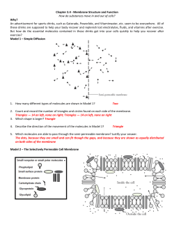


© Copyright 2026