ABC
docz
Explore
Log in
Create new account
Download
Report
No category
Modelling bilberry and cowberry yields in Finland: different
DEAL Project Final Conference: Sustainable Local Food Event (May 2015)
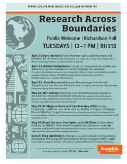
Research Across Boundaries - Forest Ecosystems & Society
the Registration Form - Kortright Centre for Conservation
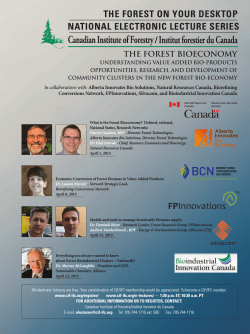
NATIONAL ELECTRONIC LECTURE SERIES THE FOREST ON
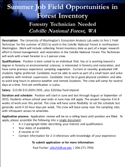
Forest Inventory Technicians
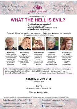
WHAT THE HELL IS EVIL?
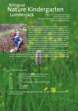
Nature Kindergarten - Lumberjack Waldkindergarten
here.
Contact: Tom Knappenberger, 503
Kerala Forests & Wildlife Department is organising an event
© Copyright 2026
About abcdocz
DMCA / GDPR
Report