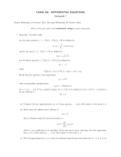
INSTITUTE OF PHYSICS PUBLISHING
JOURNAL OF PHYSICS A: MATHEMATICAL AND GENERAL
J. Phys. A: Math. Gen. 35 (2002) 9499–9515
PII: S0305-4470(02)38332-X
The spectral dimension of random trees
Claudio Destri and Luca Donetti
Dipartimento di Fisica G Occhialini, Universit`a di Milano-Bicocca and INFN, Sezione di Milano,
Piazza delle Scienze 3, I-20126 Milano, Italy
E-mail: [email protected] and [email protected]
Received 17 June 2002, in final form 9 September 2002
Published 29 October 2002
Online at stacks.iop.org/JPhysA/35/9499
Abstract
We present a simple yet rigorous approach to the determination of the spectral
dimension of random trees, based on the study of the massless limit of the
Gaussian model on such trees. As a by-product, we obtain evidence in favour
of a new scaling hypothesis for the Gaussian model on generic bounded graphs
and in favour of a previously conjectured exact relation between spectral and
connectivity dimensions on more general tree-like structures.
PACS number: 02.50.−r
1. Introduction and summary
The spectral dimension d¯ was first introduced by Alexander and Orbach [1] to characterize
the low frequency vibration spectrum of fractals. Nowadays, it is considered by most the right
generalization of the Euclidean dimension of regular lattices to irregular structures in general,
whether fractal or not, such as polymers, glasses, percolation clusters, dendritic growths and
so on. This is verified at least in many experimental situations, as well as in some theoretical
model examples, whenever the physical dimensionality explicitly enters observables such as
the spectrum of density fluctuations, the long-time properties of random walks, the critical
exponents of statistical models and many others.
In a theoretical setting, we may consider a connected graph as a model of generic irregular
structure, with physical microscopic degrees of freedom attached to the nodes and interaction
among them associated with the links. This scheme implies that the coordination of nodes is
bounded (the number of nearest neighbours of an atom, molecule or basic building block has
a geometrical upper bound) and, if the graph in question is infinite, that the surface of any Van
Hove ball (defined in terms of the chemical distance alone) must be negligible with respect to
the volume when its radius goes to infinity. In other, more physically immediate words, we
say that the structure is embeddable as a whole in a finite-dimensional Euclidean space and a
standard thermodynamic limit of infinite systems exists. We are thus led to consider bounded
graphs [2] and to study their spectral dimension.
0305-4470/02/459499+17$30.00
© 2002 IOP Publishing Ltd Printed in the UK
9499
9500
C Destri and L Donetti
To be precise, we refer here to the average spectral dimension, that is a global property
of the graph, related for instance to the infrared singularity of the Gaussian process or,
equivalently, to the density of small eigenvalues of the Laplacian or the graph average of the
long-time tail of the random walk return probability [3]. On macroscopically inhomogeneous
structures this average dimension may differ from the local one, which enters the long-time tail
of the random walk return probability on a given node [3]. However, it is the average spectral
dimension that plays the same role of the lattice Euclidean dimension in many contexts, as for
instance in providing a consistent criterion on whether a continuous symmetry breaks down
at low temperatures [4].
In this work, we address the problem of determining the average spectral dimension
of bounded trees and in particular of statistically homogeneous random trees [2] (this
homogeneity actually implies that local and average spectral dimensions coincide), which
are defined by the following branching algorithm: given a set of coordination fractions
{fz , 1 z z¯ } that are properly normalized and have average coordination 2
z¯
z=1
fz = 1
z¯
zfz = 2
(1)
z=1
an infinite random tree is built by first selecting with probability fz the coordination of the
origin and then, proceeding shell by shell away from the origin, by choosing the coordination
of every new node with probability fz except for the first node of each shell, when the modified
probability f˜z = (z − 1)fz is used to implement the non-extinction preconditioning (this is
algorithm B of [2]). These random trees represent a generalization of the incipient infinite
percolation clusters on Bethe lattices [5], since the branching probabilities are freely assigned
rather than being fixed by a single percolation probability. They also generalize to arbitrary
coordination fractions fz the infinitely large specimens of the branched polymers studied for
instance in [6].
Since the introduction of spectral dimension, the value of d¯ = 4/3 has been conjectured
for the incipient infinite percolation cluster in any dimension. This conjecture was proved
false at low dimensions, while has been considered valid in the limit of infinite dimension
(percolation on Bethe lattices). Leyvraz and Stanley [7] had in fact produced a heuristic scaling
argument in favour of d¯ = 4/3 already in 1983. Several years later, a more rigorous approach
was pursued in [6], where the branched polymer phase of two-dimensional quantum gravity
was proved to have indeed d¯ = 4/3. Branched polymers correspond to a grand canonical
ensemble of trees with all possible sizes, which is generated by a branching process like ours
above but without the non-extinction preconditioning. In this case the definition of spectral
dimension itself is subtle since such a concept does not apply to finite graphs. This is the
major difficulty in the approach of [6]. Another mathematically well-founded approach to
the problem is given in [8], where the exponent θ of the anomalous diffusion on our class
of random trees is determined as θ = 1 (the author reports only the shorter and simpler of
the two different derivations, which turns out to be more than 20 pages long, and states that
the other, more complete treatment is ‘monstrously long’). It is commonly held, although
never rigorously established in general, that θ is connected to the spectral dimension and the
(average) connectivity (or intrinsic Hausdorff ) dimension d¯c as
1
d¯
=
.
(2)
2+θ
2d¯c
Therefore θ = 1 would imply d¯ = 4/3, since d¯c = 2 for random trees [2].
In this paper, we provide a new, independent and fairly rigorous derivation of d¯ = 4/3
based on the infrared properties of the Gaussian model on our random trees (section 5).
The spectral dimension of random trees
9501
The connection of the Gaussian model with the random walk on any graph is a well-known
fact that we briefly review for completeness in section 2. As a by-product, we also obtain an
argument in favour of the conjecture (2), for any infinite graph for which the thermodynamic
limit of the Gaussian model exists: it is natural in fact to expect the scaling form
¯
µ ∼ µ0 r d c f (µ0 r γ )
(3)
for the effective squared mass of the Gaussian model in terms of a very small ‘bare’ squared
mass µ0 and the very large radius of a graph (see section 2 for the proper definitions); moreover
we also conjecture that the finite-size exponent γ coincides with 2 + θ , which is sometimes
called the random walk dimension and characterizes the scaling t ∼ r 2+θ between the time
needed by a random walker to visit with non-negligible frequency nodes at distance r from
its starting point; then the existence of the thermodynamic limit on the effective mass implies
¯
that f (x) ∼ x −d c /γ and so
1−d¯c /γ
µ ∼ µ0
¯
1−d/2
yielding exactly equation (2), since in general µ ∼ µ0
as µ0 → 0 (see section 2).
In our treatment of random trees we are indeed able to explicitly derive the scaling law
(3) with d¯c = 2 and γ = d¯c + 1 = 3, demonstrating d¯ = 4/3. It is interesting to note that if
the scaling law (3) is assumed a priori, with d¯c = 2 as well known for random trees, then the
¯ follows from a very simple ‘geometrical’
precise numerical value of γ (and therefore of d)
¯
fact: as shown in section 5, the first correction to the finite tree behaviour µ ∝ µ0 r d c comes
2d¯c +1
from the sum of squared volumes of all subtrees, which grows like r
if the volume of the
¯
tree grows like r d c . Then
2d¯c
d¯ = ¯
dc + 1
(4)
which is also a known conjecture, even with d¯c = 2, for the incipient percolation cluster and
other tree-like disordered structures [9]. Note that d¯ is monotonically increasing from 1 to
4/3 as d¯c grows from 1 to 2.
Let us observe that d¯c = 2 and d¯ = 4/3 are the greatest values among all known average
connectivity and spectral dimensions for bounded trees. This fact leads us to formulate the
following conjecture: for all bounded trees d¯c 2 and d¯ 43 , with saturation only in the case
of random trees. Evidently this must be true only for the average dimensions; there indeed
exist examples of trees (such as NTD [10]) whose local connectivity and spectral dimension,
dc and d, exceed 2 and 4/3, respectively; these present however macroscopic inhomogeneities
so that the local dimensions are different from the average ones which do satisfy the bounds
at 2 and 4/3. Let us also observe that equation (4) does not apply in the same examples if the
average dimensions are replaced by the local ones.
At the moment these upper bounds are only conjectured, but it has been rigorously proved
that d¯ 2, since bounded trees are always recurrent on the average [11].
2. Gaussian model, random walks and spectral dimension
The Gaussian model on a generic connected infinite graph G is defined [12] by assigning a
real-valued random variable φx to each node x ∈ G with the following probability distribution:


1
1
dνr [φ] =
exp−
φx (Lxy + µ0 δxy )φy 
dφx
(5)
Zr
2
x,y∈B(o,r)
x∈B(x,r)
9502
C Destri and L Donetti
for the collection φ = {φx ; x ∈ B(o, r)} relative to any Van Hove ball
B(o, r) = {y ∈ G : d(o, y) r}
o∈G
0r <∞
where d(o, y) is the chemical distance. In equation (5) Zr is the proper normalization factor
(the partition function), µ0 > 0 is a free parameter (the squared mass in field-theoretic sense)
and
Lxy = zx δxy − Axy
(6)
is (minus) the Laplacian matrix on G , zx being the coordination or degree of x and Axy the
adjacency matrix).
The thermodynamic limit is achieved by letting r → ∞ and defines a Gaussian measure
for the whole field φ = {φx ; x ∈ G } which does not depend on the centre o of the ball [13] if
G is bounded. The covariance of this Gaussian process reads
φx φy ≡ Cxy (µ0 ) = (L + µ0 )−1
xy
(7)
and setting
Cxy =
(1 − W )−1
xy
Wxy =
zx + µ0
Axy
zy + µ0
one obtains the standard connection with the random walks over G [12]:
∞
(1 − W )−1
=
(W t )xy =
W [γ ]
xy
(8)
(9)
γ :x←y
t=0
where the last sum runs over all paths from y to x, each weighted by the product along the
path of the one-step jump probabilities in W :
W [γ ] = Wxyt −1 Wyt −1 yt −2 , . . . , Wy2 y1 Wy1 y .
(10)
t
Note that, as long as µ0 > 0, we have x (W )xy < 1 for any t, namely the walker has a
nonzero death probability. This implies that Cxy is a smooth function of µ0 for µ0 > 0.
In the limit µ0 → 0 the walker never dies and the standard random walk is recovered; then
the sum over paths in equation (9) is dominated by the infinitely long paths which sample the
large scale structure of the entire graph (‘large scale’ refers here to the metric induced by the
chemical distance alone). This typically reflects itself into a singularity of Cxy at µ0 = 0.
Consider for instance a diagonal element Cxx of the covariance and suppose that its singularity
is power-like
γ = (x, yt−1 , . . . , y2 , y1 , y)
⇒
d/2−1
Sing Cxx (µ0 ) ∝ µ0
(11)
.
Then by equation (8) one sees that the same power-like behaviour appears, as λ → 1, in the
discrete Laplace transform Pxx (λ) of the random walks return probability Pxx (t) at x. In turn
this implies the long-time behaviour
Pxx (t) ∝ t −d/2
t →∞
(12)
identifying d with the local spectral dimension, which does not depend on the specific node
x [12]. To be precise the denomination ‘spectral dimension’ refers to the behaviour of the
¯
spectral density ρ(l) of low-lying eigenvalues of the Laplacian L, namely ρ(l) ∼ l d/2−1 . In
fact, it can be shown [3] that d¯ is connected to the long-time behaviour of the graph average
of Pxx (t), or equivalently to the infrared power-like singularity of the graph average C(µ0 ) of
Cxx , that is
1
¯
Cxx (µ0 ) ∝ (µ0 )d/2−1
(13)
Sing C(µ0 ) = Sing lim
r→∞ |B(o, r)|
x∈B(o,r)
The spectral dimension of random trees
9503
where |B(o, r)| is the volume of B(o, r). d¯ is therefore sometimes called the ‘average’ spectral
dimension. On regular lattices it coincides with the local spectral dimension and the usual
Euclidean dimension.
By definition, the diagonal elements Cxx of the covariance may be written as
Cxx = dϕ ϕ 2 Zx (ϕ)
(14)
where
Zx (ϕ) = lim
r→∞
dνr [φ]δ(φx − ϕ).
Thanks to the fundamental self-reproducing property of Gaussian integrations, Zx (ϕ) is
necessarily a normalized Gaussian in ϕ, that is
µ 1/2
2
x
Zx (ϕ) =
e−µx ϕ /2
2π
where, for consistency with equation (14)
1
(15)
µx (µ0 ) =
2Cxx (µ0 )
is the ‘effective mass’ at x.
3. The Gaussian model on random trees
Let us now consider the Gaussian model on an infinite bounded tree T . Any node x ∈ T may
be regarded as the root of an infinite branching process which produces T as a family tree
rooted at x. This simply means that x has as many descendants, or children, as its coordination
zx , while any other node x has zx − 1 children one step further away from the unique ancestor
x and a father one step closer to x. In particular, the zx children y of x are themselves roots of
disjoint subtrees, or branches Ty , which may or may not be infinite. Now, by the simple rules
of Gaussian integration, one easily verifies the following relation between the effective mass
at x, relative to the entire T and the effective masses at children y of x, each one relative to the
corresponding branch Ty :
µy [Ty ]
.
(16)
µx [ T ] = µ0 +
1 + µy [Ty ]
y children
of x
A similar relation holds for the effective masses µy [Ty ] in terms of the zy − 1 masses of y’s
children, and so on for the rest of the tree.
Next, suppose that the branching process is the Galton–Watson random one, with the
non-extinction preconditioning, described in the introduction (and in more detail in [2]), so
that T is an infinite random tree. Because of the preconditioning, T may be regarded as
the union of infinitely many subtrees generated by independent and identically distributed
(i.i.d.) random branching processes, without the non-extinction preconditioning, whose roots
are attached to the nodes of a half-infinite chain (the spine) that starts from x. This means that
only one of the branches at x is a priori guaranteed to extend to infinity, while the other zx − 1
are the family trees of i.i.d. random branching processes which might stop after finitely many
generations.
Let us consider first the probability distributions relative to the branching process itself
and in particular the probability Pr (µ) that the effective mass at the root x be exactly µ when
the branching algorithm is iterated for r generations, that is
Pr (µ) = δ(µx − µ)r
9504
C Destri and L Donetti
where the average is over all realizations of the tree with r generations, namely on all possible
histories of the branching algorithm with r shells completed. Taking equation (16) and the
spinal decomposition into account, we may write


z
z
µ
j
 Pr• (µ1 )
fz dµ1 dµ2 · · · dµz δ µ − µ0 −
Pr◦ (µj )
(17)
Pr+1 (µ) =
1
+
µ
j
z
j =1
j =2
where P ◦ (µ) is the same probability without the non-extinction preconditioning and fulfils
the functional recursion


z−1
z−1
µ
j 
◦
(µ) =
fz dµ1 dµ2 · · · dµz−1 δ µ − µ0 −
Pr◦ (µj )
(18)
Pr+1
1
+
µ
j
z
j =1
j =1
while Pr• (µ) is the probability when also the coordination of the root is extracted with the
modified probability f˜z and satisfies therefore


z−1
z−1
µ
j  •
•
Pr (µ1 )
Pr+1
f˜z dµ1 dµ2 · · · dµz−1 δ µ − µ0 −
(µ) =
Pr◦ (µj ). (19)
1
+
µ
j
z
j =1
j =2
As r → ∞ we expect all these probability distributions to converge to their limiting forms
◦
•
P∞ (µ), P∞
(µ) and P∞
(µ), turning equations (17), (18) and (19) into highly nontrivial coupled
◦
•
integro-functional equations for P∞ (µ), P∞
(µ) and P∞
(µ) with a parametric dependence on
µ0 . In particular, we are interested in their infrared behaviour as µ0 → 0.
4. Statistical homogeneity and auto-averaging property
Before addressing the problem just mentioned, we need to establish the precise relation with
the original problem, that of determining the µ0 → 0 behaviour of C(µ0 ) on a given ‘generic’
infinite random tree T produced by our algorithm. By ‘generic’ in this context we mean
an infinite T belonging to the subset of unit measure of trees that fulfil the auto-averaging
property for local observables. To be explicit, consider the frequency F (r, τ ) of occurrence in
T of a given rooted tree τ with r generations. In terms of the Van Hove balls B(x, r), regarded
as subtrees of T , we may write F (r, τ ) as the graph average
1
FR (r, τ ) =
δ[B(x, r) = τ ]
F (r, τ ) = lim FR (r, τ )
R→∞
|B(o, R)|
x∈B(o,R)
where o is an arbitrary node of T and δ[τ = τ ] is one if its argument is a true statement and
zero otherwise. F (r, τ ) does not depend on the choice of o (T is a bounded graph) and it is
convenient to identify o as the root, or origin, of the infinite branching algorithm.
Let us then recall that any T produced by the algorithm may be decomposed into the
spine S (the origin o plus all the nodes on which the coordination was extracted with f˜z ) and
the transverse family trees of the identical, independent and non-preconditioned branching
processes starting from the nodes of the spine (see [2, 8] for more details). Evidently, the
intersection of the transverse family trees rooted at s ∈ S with B(o, R) contains at most
R − d(s, o) generations, so that they contribute differently, even on average, to FR (r, τ ).
Therefore, to simplify our derivation, we consider a modified thermodynamic limit, in which
the infinite tree is not recovered through a Van Hove ball with diverging radius, but as R → ∞
limit of the set
ωs,R
R =
s∈SR
The spectral dimension of random trees
9505
where SR is the restriction of the spine to the first R generations of T and ωs,R is the union of
all transverse family trees rooted at s and restricted to the first R generations. Thus we redefine
FR (r, τ ) as
|ωs,R |
FR (r, τ ) =
ws,R Qs,R (r, τ )
ws,R =
|R |
s∈S
R
Qs,R (r, τ ) =
1
δ[B(x, r) = τ ].
|ωs,R | x∈ω
s,R
Note that, by construction, the random weights ws,Rare all identically distributed and are all
independent except for the normalization constraint s∈SR ws,R = 1. The random frequencies
Qs,R (r, τ ) are all identically distributed, but are not independent because a ball B(x, r) will
>
in general intersect several ωs,R if d(x, s) < r. Therefore we split ωs,R into ωs,R
, formed by
nodes x such that d(x, s) > r, and its complement ωs , which does not depend on R for large
R. This implies an analogous splitting for the random weights and the random frequencies.
Now the random frequencies Q>
s,R (r, τ ) are all independent since the two events B(x, r) = τ
>
and B(x , r) = τ are independent if x ∈ >
s,R and x ∈ s ,R with s = s . Note also that
Qs,R (r, τ ) and ws ,R are independent when s = s .
Thus we have
FR (r, τ ) = FR (r, τ ) + FR> (r, τ )
with FR (r, τ ) getting contributions solely from nodes at distances not larger than r from the
spine. Clearly, in the limit R → ∞, these nodes form a subset of zero measure of T , since
¯
s ωs (r, τ ) is essentially one dimensional while a generic T has d c = 2. Hence, as R → ∞,
F (r, τ ) = lim FR> (r, τ ).
R→∞
By analogous dimensionality arguments we get that almost always limR→∞ ws,R = 0, although
the sum of all these random weights stays properly normalized.
We may now invoke directly the law of large numbers for FR> (r, τ ), which is the weighted
average of i.i.d. random variables. Hence, for any finite r, F (r, τ ) is almost always nonfluctuating on infinite trees and
F (r, τ ) = Q> (r, τ )◦
◦
where Q> (r, τ ) is any one of the limR→∞ Q>
s,R (r, τ ) and the average · is taken with respect
to the algorithm without the preconditioning on non-extinction. But any node x on such
trees lying at a distance larger then r from the origin enjoys statistical homogeneity for the
event B(x, r) = τ , since the branching is i.i.d. on every node (but the origin, at most) and
B(x, r) = τ cannot contain the origin. Moreover, the unique path connecting x to o plays the
role of the spine for a branching process rooted at x and preconditioned on non-extinction for
at least r generations, since the trees contributing to Q> (r, τ )◦ have at least r generations.
We conclude therefore that almost always an infinite random tree T has the auto-averaging
property
F (r, τ ) = δ[B(o, r) = τ ]
(20)
with respect to the probability itself that the first r shells of T build up to form the given finite
tree τ . Then this property holds for any local observable and in particular for the effective mass
µx [B(x, r)] of a Gaussian model restricted to B(x, r). Thus the probability distribution Pr (µ)
coincides with the frequency of the event µx [B(x, r)] = µ, as x varies throughout a ‘generic’
infinite random tree T . The same would evidently apply to the probability distribution of the
variable (2µ)−1 and the frequency of the event Cxx [B(x, r)] = (2µ)−1 .
9506
C Destri and L Donetti
5. Scaling
Let us now return to the recursion relations (17), (18) and (19) for the probability distributions
Pr (µ), Pr◦ (µ) and Pr• (µ), respectively. We are interested in the thermodynamic limit r → ∞
of infinite trees followed by the massless limit µ0 → 0. These two limits can actually be
applied simultaneously, provided we identify the correct scaling variables. Suppose in fact
that, as r → ∞ and µ, µ0 → 0, the scaling law (3) applies; since µ is really a random
variable, a better formulation is in terms of its probability, that is
β β
(21)
Pr (µ; µ0 ) µ0 F µµ0 , µ0 r γ
for suitable scaling exponents β and γ and scaling function F (u, s). β is then directly related
¯ thanks to equation (11), the results of the previous
to the spectral dimension, as β = −1 + d/2,
section and the existence of the thermodynamic limit; γ provides instead a measure of finitesize effects at very large sizes. In particular, if we let µ0 → 0 too fast, so that µ0 r γ → 0 even
if r → ∞, we must recover the massless behaviour characteristic of finite trees. This amounts
to linearizing the effective mass formula (16), so that
µx [T ] = µ0 v[T ]
where v[T ] is the volume of T . Thus
−1 ˆ
ˆ
Pr (µ; µ0 ) µ−1
0 P r (µ/µ0 ) = µ0 P r (v)
where Pˆ r (v) is the volume probability at radius r, which for large r has a scaling form in
terms of v/r 2 explicitly determined in [2] (thus implying d¯c = 2). Since this scaling form is
highly nontrivial, with exponentially small behaviour also for v/r 2 → 0, compatibility with
the scaling hypothesis (21) requires 1 + β = 2/γ , that is
d¯
d¯
1
= = ¯ .
γ
4
2d c
One is therefore led to the identification (compare with equation (2) in the introduction)
γ = 2+θ
relating finite-size effects to the exponent of anomalous diffusion. Of course, since relation (2)
is only a well-founded conjecture, an explicit derivation of γ = 2 + θ would provide a proof of
the conjecture for our random trees. Let us stress the point: γ measures the scaling behaviour
of the Gaussian model (and therefore of the random walk) on finite random trees of very large
radius r; 2 + θ characterizes instead the scaling t ∼ r 2+θ between the time needed by a random
walker to visit with non-negligible frequency nodes at distance r from its starting point. The
two concepts are certainly related but quite distinct, so that the identification γ = 2 + θ has a
nontrivial content.
Let us come back now to the opposite limiting behaviour of the probability distributions
β
that is the subject of this work, namely r → ∞ and µ, µ0 → 0 with u = µµ0 fixed and
γ
s = µ0 r finite and possibly very large. We shall show now that the scaling law (21) is indeed
correct with the precise values
β = −1/3
γ =3
(22)
implying d¯ = 4/3. The detailed proof, by induction on all moments of Pr (µ), Pr◦ (µ) and
Pr• (µ), is rather simple albeit notationally a bit cumbersome and is reported in the appendix.
Here we only provide a sketch of the derivation.
The first step consists in rewriting the recursion relations (17), (18) and (19) into a more
tractable form. In fact they are amenable to a direct treatment via Laplace transform only in
The spectral dimension of random trees
9507
the limit µ0 → 0 at fixed r, while we are interested in a regime where the nonlinearity in the
effective mass formula (16) plays a crucial role. Therefore we consider the expansion in all
powers of µ0
µx [ T ] =
∞
(−1)n+1Vn (x)µn0
(23)
n=1
where the coefficients Vn (x) are integer-valued random variables satisfying composition laws
obtained by equating powers of µ0 on both sides of equation (16). These read
V1 (x) = 1 +
V1 (y)
y children
of x
[V2 (y) + V1 (y)2 ]
V2 (x) =
V3 (x) =
V4 (x) =
y children
of x
y children
of x
[V3 (y) + 2V1 (y)V2 (y) + V1 (y)3 ]
[V4 (y) + 2V1 (y)V3 (y) + V2 (y)2 + 3V1 (y)2 V2 (y) + V1 (y)4 ]
y children
of x
V5 (x) = · · ·
which we write in general as
Vn (x) = δn,1 +
Fn (V1 (y), V2 (y), . . . , Vn (y))
(24)
y children
of x
where the form of Fn can be easily induced from the previous formulae. Note that V1 can
be interpreted as the volume of the subtree, V2 as the sum of the squares of all sub-volumes
and so on. Now we may write recursion relations for the probability of the coefficients Vn (x)
themselves. For instance, in the branching algorithm without non-extinction preconditioning,
we have
◦
(V1 , . . . , Vn ) =
Pr+1
fz
z
×
n
k=1

z−1
V1,1 ,...,V1,z−1 i=1
V2,1 ,...,V2,z−1
···
Vn,1 ,...,Vn,z−1
δ Vk − δn,1 −
z−1
Pr◦ (V1,i , . . . , Vn,i )

Fk (V1,j , . . . , Vk,j )
(25)
j =1
with similar expressions for probabilities Pr (V1 , . . . , Vn ) and Pr• (V1 , . . . , Vn ) corresponding
to those for the effective mass Pr (µ) and Pr• (µ). For brevity we do not write them here; they
can be found in the appendix.
The advantage of this new formulation lies in the fact that Fn ({V1,i , . . . , Vn,i ) is by
construction linear in Vn,i . This allows us to set up a systematic control of the large r behaviour
of the recursion relations for the multiple moments of Pr (V1 , . . . , Vn ), Pr◦ (V1 , . . . , Vn ) and
Pr• (V1 , . . . , Vn ). Consider for example the lowest moments: from equation (25) and its
analogues in the appendix we get
9508
C Destri and L Donetti
V1 ◦r+1 =
fz (1 + (z − 1)V1 ◦r ) = 1 + V1 ◦r
z
V1 •r+1
=
(z − 1)fz (1 + V1 •r + (z − 2)V1 ◦r ) = 1 + V1 •r + g (1)V1 ◦r
z
V1 r+1 =
fz (1 + V1 •r + (z − 1)V1 ◦r ) = 1 + V1 •r + V1 ◦r
z
where g(λ) is the so-called probability generating function
fz λz−1 = f1 + f2 λ + f3 λ2 + · · ·
g(λ) =
(26)
z
which thanks to equations (1) enjoys the properties
g (1) = 1.
g(1) = 1
(27)
Hence we obtain the asymptotic behaviour for large r
V1 ◦r ∼ r
V1 r ∼ V1 •r ∼ r 2
(28)
which implies d¯c = 2 since V1 is just the volume. Next consider the averages of V2 and V12 ;
the recursion rules read
◦ ◦
(z − 1)fz V2 ◦r + V12 r = V2 ◦r + V12 r
V2 ◦r+1 =
V2 •r+1 =
z
•
◦ (z − 1)fz V2 •r + V12 r + (z − 2)V2 ◦r + (z − 2) V12 r
z
V2 r+1
•
◦
= V2 •r + V12 r + g (1)V2 ◦r + g (1) V12 r
•
◦
= V2 •r + V12 r + V2 ◦r + V12 r
and
2 ◦
◦
V1 r+1 = 1 + V12 r + g (1)(V1 ◦r )2 + 2V1 ◦r
•
◦
2 •
V1 r+1 = 1 + V12 r + 2V1 •r + g (1) V12 r + V1 ◦r V1 •r + 2V1 ◦r + g (1)(V1 ◦r )2
2
•
◦
V1 r+1 = 1 + V12 r + 2V1 •r + V12 r + V1 ◦r V1 •r + 2V1 ◦r + g (1)(V1 ◦r )2 .
We can read right away the r → ∞ asymptotic behaviour
2 ◦
V1 ∼ r 3
2 r
V1 r ∼ r 4
V2 ◦r ∼ r 4
(29)
V2 r ∼ r .
(30)
5
Evidently the moments of Pr• (V1 , . . . , Vn ) all have the same asymptotic behaviour as those of
Pr (V1 , . . . , Vn ) and need not be written out explicitly.
Let us make use of the results (28) and (29) for the mean value of the effective mass at
the root o:
∞
µr =
(−1)n+1 Vn r µn0 µ0 r 2 (c0 + c1 µ0 r 3 + · · ·)
(31)
n=1
where c0 and c1 are constants. If we assume the scaling law (21) for the probability Pr (µ; µ0 ),
then clearly
γ
µr µ−β
o F1 (µ0 r )
The spectral dimension of random trees
9509
with F1 (s) finite in the limit s → ∞; consistency with (31) now requires that F1 (s) ∼
s 2/γ (1 + O(s 3 )) as s → 0 to reproduce the correct r behaviour on large but finite trees; but
matching also the powers of µ0 implies
1 + β = 2/γ
2 + β = 5/γ
yielding exactly the desired result (22). This argument may be turned around to avoid
referring to the scaling hypothesis (21) for the probability and to better clarify the role of the
thermodynamic limit. In fact, the first two terms of the µ0 -expansion in (31) suggest that, as
r → ∞ and µ0 → 0 at fixed µ0 r 3 ,
µr µ0 r 2 G1 (µ0 r 3 )
(32)
for a suitable scaling function G1 (s). Now the existence of the thermodynamic limit [12]
1/3
requires that G1 (s) ∼ s −2/3 for large s, yielding again µ∞ ∼ µ0 , that is β = −1/3. Of
course this formulation is only tentative, since we still need to verify that, for any other n > 2,
the nth term in the µ0 -expansion of µr contains r 3n+2 as the highest power of r. Moreover,
even if we can prove the scaling (32) of µr , this does not imply the scaling (21) for the whole
probability Pr (µ; µ0 ). In the appendix we demonstrate by induction that, as r → ∞
k
Vnj ∼ r 3 j nj −k [1 + O(r −1 )].
(33)
j =1
r
Hence, by retaining only the dominant r behaviour, we have
3i+2
+ · · · µ0 r 2 G1 (µ0 r 3 )
µr c0 µ0 r 2 + c1 µ20 r 5 + c2 µ30 r 8 + · · · + ci µi+1
0 r
and, by the same token
µ2 r =
∞
(−1)k µk0
k=2
k−1
Vj Vk−j r µ20 r 4 G2 (µr 3 ).
j =1
Similarly one obtains for any n
µn r µn0 r 2n Gn (µ0 r 3 )
so that, requiring the existence of the thermodynamic limit, one obtains as µ0 → 0+ at r = ∞
n/3
µn ≡ lim µn r = bn µ0
r→∞
where
bn = lim s 2n/3 Gn (s).
s→∞
We may also reformulate this result as
n/3
µn r µ0 Fn (µ0 r 3 )
where Fn (s) = s 2n/3 Gn (s) has a finite nonzero limit as s → ∞. This general form of the
moments of Pr (µ; µ0 ) implies the scaling form (21) with β = −1/3, γ = 3 and
Fn (s) = du un F (u, s)
for the probability Pr (µ; µ0 ) itself.
Let us close this section with one more observation concerning the universality of the
scaling law (3) or (21) with respect to the coordination distribution defined by the fz numbers
or, equivalently, by the probability generating function g(λ). A more careful analysis of the
9510
C Destri and L Donetti
Pintegrated = 0.05, 0.2, 0.5, 0.8, 0.95
r = 250
r = 500
r = 1000
r = 2000
r = 4000
0
u
10
–1
10
–2
10
–2
10
0
10
2
10
4
10
6
10
s
Figure 1. Lines of constant integrated probability from the numerical data.
dominant large r terms in the recursion rules for Vn expectations shows that (see the appendix
for details)
k
Vnj ∼ α j nj r 3 j nj −k
j =1
r
where α = g (1) measures the fluctuations of the coordinations since
(z − 2)2 fz .
α=
z
We may therefore refine the scaling law (21) to
Pr (µ; µ0 ) (αµ0 )−1/3 F ((αµ0 )−1/3 µ, αµ0 r 3 )
(34)
where F (u, s) is a universal scaling function.
6. Numerical checks
As an extra check on our derivation and to determine the profile of the universal function
F (u, s), we numerically evaluated Pr (µ; µ0 ) by directly calculating the effective mass µ for
each member of a large set of trees produced by our branching algorithm. For each one of the
selected values of µ0 and r we obtained several thousand values of µ that may be arranged into
a histogram providing a discretized estimate of Pr (µ; µ0 ) dµ. This procedure does not require
much computer time or memory thanks to the recursive structure of the mass composition
formula (16). Our results for the integrated probability at the five values 0.05, 0.2, 0.5, 0.8 and
−1/3
0.95 are plotted in figure 1 using the scaling variables u = µ0 µ and s = µ0 r 3 (with our
specific choice of fz we have α = 1). The data show a very good scaling profile with a very
well-defined crossover, as s gets larger, from the behaviour typical of small trees, µ ∝ µ0 ,
1/3
to that characteristic of large trees, that is µ ∝ µ0 . The vertical section of the data at
The spectral dimension of random trees
9511
0.16
r = 5000
4
s ∼ 10
0.14
0.12
F(u,s)du
0.1
0.08
0.06
0.04
0.02
0
0
0.5
1
1.5
2
2.5
3
3.5
4
u
Figure 2. Numerical distribution for F(u, s) for 10 000 random trees.
s 104 provides a good estimate of the probability distribution F (u, ∞) du and is reported
in figure 2.
7. Conclusions and outlook
Let us remark once more on the two distinct levels of our approach: our proof by induction of
equation (33) provides a rigorous basis for the scaling form (21) of Pr (µ; µ0 ) with β = −1/3
and γ = 3. Thanks to the auto-averaging property, this implies in turn that indeed
¯
d/2−1
d¯ = 4/3.
Sing C(µ0 ) ∝ µ0
Moreover, due to the statistical homogeneity of our random trees, we see that the local and
average spectral dimensions coincide. On the other hand, if we assume scaling, as natural and
common in this context, then the determination d¯ = 4/3 follows solely and very simply from
the large r asymptotic behaviour of V2 r , that is the average of the sum of squared volumes
¯
of all subtrees of the tree. Since the volume V1 scales as r d c , with d¯c = 2, then V2 must scale,
2d¯c +1
; then
almost by definition, as r
¯
¯
µr µ0 r d c (c0 + c1 µ0 r d c +1 + · · ·)
which is consistent with scaling only if
2d¯c
d¯ =
.
(35)
d¯c + 1
Note that this holds true even if d¯c < 2, as could happen for different types of bounded trees.
We conjectured in [2] that d¯c 2 for any bounded tree, with saturation only for random trees.
Then automatically d¯ 4/3 for any bounded tree, with saturation only for random trees. The
general expression (35) was conjectured years ago from very different considerations [9].
Another relevant issue concerns the spectral weight w¯ of infinite random trees. This is
¯
d/2−1
singularity of C(µ0 ) as µ0 → 0, that is
the coefficient of the µ0
−1/3
C(µ0 ) ∼ wµ
¯ 0
.
9512
C Destri and L Donetti
It is clear from equation (15) and the auto-averaging property that the spectral weight is related
to the scaling function F (u, s) by
du
F (u, ∞).
w¯ =
2u
On the other hand, it is known [12] that on any given infinite graph with local spectral
dimension d < 2, the local spectral weight does not really depend on x, that is
d/2−1
Cxx (µ0 ) ∼ wµ0
(36)
for any node x. Moreover, thanks to statistical homogeneity, it is clear that on a given tree
w = (2u)−1 , with u a specific instance of a random variable distributed according to F (u, ∞).
Since F (u, ∞) is not δ-like (see the previous section), we have in general w = w,
¯ that is the
local and average spectral weights differ in general, unlike the spectral dimension. One might
wonder then about the auto-averaging property, since w does not fluctuate over the tree. Of
course the resolution of this apparent contradiction is in the order of limits: averaging over the
infinite graph and small µ0 asymptotics of Cxx (µ0 ) are operations that cannot be commuted
in general.
These last remarks suggest a further development in the explicit calculation of the universal
limit function F (u, ∞). Another interesting direction of research is in the construction of
modified tree-generating algorithms such that scaling is preserved with d¯c < 2, in order to
check the general formula (35).
Acknowledgments
We thank R Burioni and D Cassi for many valuable comments and suggestions.
Appendix. Asymptotic behaviour of moments
First of all let us write the explicit form of Fn
Fn (V1 , V2 , . . . , Vn ) = Vn +
n−1
n ···
k=2 n1 =1
n−1

δ n −
nk =1
k
j =1

ni 
k
Vnj .
j =1
In the case without the non-extinction condition we will prove that
k
◦
Vnj ∼ α j nj −1 r 3 j nj −k−1 .
j =1
(A1)
r
First of all let us prove this equation when all nj = 1; the case k = 1 is known from
equation (28) while for arbitrary k is proved by induction; in fact if
j ◦
V1 r ∼ α j −1 r 2j −1
(A2)
is assumed for j k we have
k+1 ◦
V1 r+1 =
fz
z
=
1+
V1,1 ,V1,2 ,...,V1,z−1
z
fz
V1,1 ,V1,2 ,...,V1,z−1
z−1
V1,i
k+1 z−1
i=1
Pr◦ (V1,i )
i=1
k+1
V1,i
+k
k
V1,i
+ ···+ 1
z−1
i=1
Pr◦ (V1,i )
The spectral dimension of random trees
9513
k
k+1 ◦
j ◦ k+1−j ◦
= V1 r + α
V1 r V1
r
j =1
k
+ g (1)
j1 ,j2 ,j3 =1
j1 ◦ j2 ◦ j3 ◦
V1 r V1 r V1 r δ(k + 1 − j1 − j2 − j3 ) + · · ·
k
◦
j ◦ k−j ◦
+ k V1k r + α
V1 r V1 r + lower order terms
j =1
◦
∼ V1k+1 r + α k r 2k
(A3)
where all addends which
consist
of a product of three or more averages and those that come
from lower powers of
V1,i are negligible in the limit r → ∞ thanks to equation (A2), so
that
k+1 ◦
V1 r ∼ α (k+1)−1 r 2(k+1)−1
extending equation (A2) from k to k + 1.
Now,
let us prove equation (A1) by induction; in this case the induction is on the quantity
N = 3 kj =1 nj − k. Let us denote by n¯ the greatest among n1 , n2 , . . . , nk ; we have
z−1
◦
k
k
z−1
Vnj
=
fz
Fnj V1,i , . . . , Vnj ,i
Pr◦ (V1,i , . . . , Vn,i
δnj ,1 +
¯ )
j =1
V1,1 ,...,V1,z−1 j =1
V2,1 ,...,V2,z−1
···
Vn¯ ,1 ,...,Vn¯ ,z−1
z
r+1
=
k
◦
+
Vnj
j =1
+α
∼
r
k
k n
j −1
j =1
Vl Vnj −l
Vnj
+α
Vnj
j =1 l=1
◦ j ∈S
◦
S
i=1
r
j
◦
nj −1 3
j =j
◦
Vnj r
+ lower order terms
Vnj
j ∈S
/
i=1
r
r
j
nj −k−2
r
where S are all the possible ordered subsets of {n1 , n2 , . . . , nk }. Now equation (A1) follows
but a few remarks are needed. First, all terms on the right-hand side involve averages whose
value of N is smaller than those on the left-hand side. Then all the terms that are not explicitly
written are proportional to lower powers of r: some of them in fact consist of the product
of three or more averages (each of them carries a ‘−1’ in the exponent), some others are
expressions with more than k + 1 factors Vn , and finally some others come from products
involving the δnj ,1 .
We turn now to the probability P • (V1 , . . . , Vn ) with non-extinction condition for which
the recursion reads
z−1
•
f˜z
(V1 , . . . , Vn ) =
Pr• (V1,1 , . . . , Vn,1 )
Pr◦ (V1,i , . . . , Vn,i )
Pr+1
z
×
n
k=1

V1,1 ,...,V1,z−1
V2,1 ,...,V2,z−1
···
Vn,1 ,...,Vn,z−1
δ Vk − δn,1 −
z−1
j =1
i=2

Fk (V1,j , . . . , Vk,j ) .
9514
C Destri and L Donetti
We will prove that
k
•
∼α
Vnj
j =1
j
nj 3
r
nj −k
j
(A4)
.
r
Some special cases, including k = n1 = 1 have already been
shown in section 5, while the
•
general case is proved by induction. In fact the recurrence for kj =1 Vnj r reads (writing only
leading order terms, as before)
k
•
k
z−1
Vnj
=
(z − 1)fz
Fnj V1,i , . . . , Vnj ,i
δnj ,1 +
j =1
V1,1 ,...,V1,z−1 j =1
V2,1 ,...,V2,z−1
···
Vn¯ ,1 ,...,Vn¯ ,z−1
z
r+1
z−1
× Pr• (V1,1 , . . . , Vn,1
¯ )
k
=
+
j =1
+α
r
k
∼
k n
j −1
j =1 l=1
• Vnj
j ∈S
•
S
j =1
j
nj 3
r
Vl Vnj −l
•
+α
Vnj j =j
◦
k
◦
Vnj
j =1
r
r
+ lower order terms
Vnj
j ∈S
/
r
+α
Vnj
Pr◦ (V1,i , . . . , Vn,i
¯ )
i=2
•
Vnj
i=1
r
j
nj −k−1
r
with the same remarks as in the previous case.
Finally the recursion for the probability P (V1 , . . . , Vn ) reads
Pr+1 (V1 , . . . , Vn ) =
fz
z
n
×

Pr• (V1,1 , . . . , Vn,1 )
V1,1 ,...,V1,z
V2,1 ,...,V2,z
···
Vn,1 ,...,Vn,z
z
Pr◦ (V1,i , . . . , Vn,i )
i=2
δ Vk − δn,1 −
z

Fk (V1,j , . . . , Vk,j )
j =1
k=1
and, following the same steps as before,
k
k
z
Vnj
=
fz
Fnj V1,i , . . . , Vnj ,i
δnj ,1 +
j =1
z
r+1
V1,1 ,...,V1,z j =1
V2,1 ,...,V2,z
···
Vn¯ ,1 ,...,Vn¯ ,z
i=1
× Pr• (V1,1 , . . . , Vn,1
¯ )
=
Vnj + lower
j =1
r
j nj 3
j nj −k
∼α
r
Pr◦ (V1,i , . . . , Vn,i
¯ )
i=2
•
k
z
.
order terms
The spectral dimension of random trees
References
[1]
[2]
[3]
[4]
[5]
[6]
[7]
[8]
[9]
[10]
[11]
[12]
[13]
Alexander S and Orbach R 1982 J. Phys. Lett. 43 625
Destri C and Donetti L 2002 J. Phys. A: Math. Gen. 35 5147
Burioni R and Cassi D 1996 Phys. Rev. Lett. 76 1091
Cassi D 1996 Phys. Rev. Lett. 76 2941
Burioni R, Cassi D and Vezzani A 1999 Phys. Rev. E 60 1500
Essam J W 1980 Rep. Prog. Phys. 43 833
Jonsson T and Wheater J F 1998 Nucl. Phys. B 515 549
Leyvraz F and Stanley E 1983 Phys. Rev. Lett. 51 2048
Kesten H 1987 Ann. Inst. H Poincar´e B 22 425
Havlin S and Ben-Avraham D 1987 Adv. Phys. 36 695–798
Burioni R and Cassi D 1995 Phys. Rev. E 51 2865
Donetti L 2002 Preprint cond-mat/0206149
Hattori K, Hattori T and Watanabe H 1987 Prog. Theor. Phys. Suppl. 92 108
Burioni R, Cassi D and Vezzani A 1999 J. Phys. A: Math. Gen. 32 5539
9515