ABC
docz
Explore
Log in
Create new account
Download
Report
technology and computing
internet technology
web search
REVISITING GUIDED IMAGE FILTER BASED STEREO MATCHING AND SCANLINE
QXT-700 Quad Core HD Touch Screen / Controller
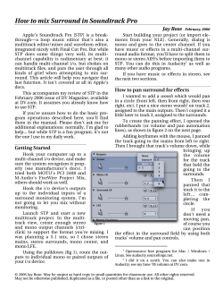
How to mix Surround in Soundtrack Pro Jay Rose
Document 333491
AUCTION SATURDAY, NOV. 1 • 9:30 A.M. OWNER: JACI MORGAN
CHEVERNY II-XLR Prestigious symmetric audio stereo cable
How To Teach Stereoscopic Matching? (Invited Paper) Radim ˇS´ara
Large-Scale Dense 3D Reconstruction from Stereo
A/V Extender (100m) EOC-VA1H
Guidance on how to complete our application form
Measurement of Micro-bathymetry with a GOPRO Underwater Stereo Camera Pair
Elevation-Based MRF Stereo Implemented in Real
Cortical mechanisms of binocular stereoscopic vision
© Copyright 2026
About abcdocz
DMCA / GDPR
Report