
DOES WORKING FROM HOME WORK? EVIDENCE FROM A CHINESE EXPERIMENT
DOES WORKING FROM HOME WORK? EVIDENCE FROM A CHINESE EXPERIMENT Nicholas Blooma, James Liangb, John Robertsc and Zhichun Jenny Yingd November 6, 2014 Abstract: A rising share of employees now regularly work from home (WFH), but there are concerns this can lead to “shirking from home.” We report the results of a WFH experiment at Ctrip, a 16,000employee, NASDAQ-listed Chinese travel agency. Call center employees who volunteered to WFH were randomly assigned either to work from home or in the office for 9 months. Home working led to a 13% performance increase, of which 9% was from working more minutes per shift (fewer breaks and sick days) and 4% from more calls per minute (attributed to a quieter and more convenient working environment). Home workers also reported improved work satisfaction and their attrition rate halved, but their promotion rate conditional on performance fell. Due to the success of the experiment, Ctrip rolled out the option to WFH to the whole firm and allowed the experimental employees to re-select between the home and office. Interestingly, over half of them switched, which led to the gains from WFH almost doubling to 22%. This highlights the benefits of learning and selection effects when adopting modern management practices like WFH. Keywords: working from home, organization, productivity, field experiment, and China Acknowledgements: We thank Jennifer Cao, Mimi Qi and Maria Sun from Ctrip for data, advice and logistical support. We thank Chris Palauni, David Butler, Jared Fletcher and Michelle Rowan for their time discussing home-working and the call-center industries. We thank our formal discussants Mushfiq Mobarak, Rachael Heath, Sabrina Pabilonia, Shing-Yi Wang, our editors (Larry Katz and Andrei Shleifer) and our four anonymous referees, and numerous seminar audiences for many helpful comments. We thank the National Science Foundation and Toulouse Network for Information Technology (which is supported by Microsoft) for co-funding for this project. Conflict of interest and IRB statement: No funding was received from Ctrip. James Liang is the cofounder of Ctrip. During the experiment we report here he was non-executive Chairman of Ctrip. Since the end of the experiment he has returned to Ctrip as CEO. No other co-author has any financial relationship with Ctrip. Neither the results nor the paper were pre-screened by anyone. The experiment received Stanford IRB approval. The IRB did not require changes in our experimental design. a Stanford Economics, SIEPR, CEPR and NBER; b Beijing University Guanghua Management School and Ctrip, c Stanford GSB and SIEPR, d Stanford Economics and Cornerstone Research. 1 I. INTRODUCTION Working from home (also called telecommuting or telework, but hereafter referred to as “WFH”) is becoming an increasingly common practice. In the United States, the proportion of employees who primarily work from home has more than tripled over the past 30 years, from 0.75% in 1980 to 2.4% in 2010 (Mateyka et al. 2012).1 At the same time, the wage discount (after controlling for observables) from primarily working at home has fallen, from 30% in 1980 to zero in 2000 (Oettinger, 2011). Home-based workers now span a wide spectrum of jobs, ranging from sales assistants and realtors to managers and software engineers, with a correspondingly wide range of incomes (Figure I).2 Internationally, working from home also appears to be common. Figure II shows the share of managers allowed to “work from home during normal working hours”, from a major telephone survey we ran on over 3,000 medium sized (50 to 5000 employee) manufacturing firms during 2012-2013.3 This is a broader measure of WFH as it covers managers that are allowed to WFH occasionally, for example, one day a week. We find two interesting findings. First, the share of managers in the US, UK and Germany allowed to WFH during normal hours is almost 50%, signaling this is now a mainstream practice. Second, the share in many developing countries is surprisingly high, at 10% or 20%. Survey respondents from developing countries told us that WFH is becoming increasingly common because of rising traffic congestion and the spread of laptops and cell-phone connectivity. Having employees work from home raises two major issues. First, is it a useful management practice for raising productivity and profitability? This is an important question that lacks systematic evidence or consensus. Even within a single industry practices often vary dramatically. For example, at JetBlue Airlines, call-center employees all work from home, American Airlines does not allow any home work, and United Airlines has a mix of practices. More generally, Bloom et al. (2009) reported wide variation in the adoption rates of managers and employees of WFH within every 3-digit SIC industry code surveyed. The second issue relates to the concerns over deteriorating work-life balance and the potential of working from home to help address this. The share of US households with children in which all parent(s) were working has increased from 40% in 1970 to 62% by 2012 (Council of Economic Advisors, 2014). The increasing pressure for parents to work is leading governments in the US and Europe to investigate ways to promote work-life balance, with again a shortage of evidence: A factor hindering a deeper understanding of the benefits and costs of flexibility is a lack of data on the prevalence of workplace flexibility and arrangements, and more research is needed on the mechanisms through which flexibility influences workers’ job satisfaction and firms’ profits to help policy makers and managers alike. 1 This share was 1% in 1990 and 1.4% in 2000, so has been steadily increasing. Our experiment studies call-center employees, who are in lower income deciles, while professionals, managers and even academics would be typical of those in the top deciles. Interestingly, the polarization of WFH into top and bottom deciles looks similar to broad employment trends (e.g. Autor, Katz and Kearney, 2006) 3 This data comes from questions included in recent waves of management surveys following the survey protocol outlined in Bloom and Van Reenen (2007) and Bloom et al. (2014). 2 2 (Council of Economic Advisors, 2010, Executive Summary) The efficacy of WFH as a management practice was what concerned Ctrip, China’s largest travel agency, with 16,000 employees and a NASDAQ listing. Its senior management was interested in allowing its Shanghai call-center employees to work from home because they perceived potential benefits from reducing office rental costs, which were increasing rapidly due to the booming real estate market in Shanghai. They also thought that allowing WFH might reduce the high attrition rates the firm was experiencing by saving the employees from long commutes. But the managers worried that allowing employees to work at home, away from the direct oversight of their supervisors, would lead to a large increase in shirking. The call center workforce was mainly younger employees, many of whom might well have been expected to struggle to remain focused working from home without direct supervision. Given the uncertainty surrounding the effects of working from home in the research literature as well as in practice, the firm’s senior management decided to run a randomized controlled trial. The authors assisted in designing the experiment and, essentially whenever feasible, our recommendations were followed by management. We had complete access to the resulting data, as well as to data from surveys conducted by the firm. We also conducted various surveys ourselves and numerous interviews with employees, line supervisors and senior management. In summary, Ctrip decided to run a nine-month experiment on working from home. They asked the 996 employees in the airfare and hotel departments of the Shanghai call center whether they would be interested in working from home four days a week, with the fifth day in the office. 4 Approximately half of the employees (503) were interested, particularly those who were married, had children and faced long commutes. Of these, 249 were qualified to take part in the experiment by virtue of having at least six months tenure, broadband access and a private room at home in which they could work. After a lottery draw, those employees with even-numbered birthdays were selected to work from home, while those with odd-numbered birthdates stayed in the office to act as the control group. Office and home workers used the same IT equipment, faced the same work order flow from a common central server, carried out the same tasks and were compensated under the same pay system, which included an element of individual performance pay. Hence, the only difference between the two groups was the location of work. This allows us to isolate the impact of working from home versus other practices that are often bundled alongside this practice in attempts to improve work-life balance, such as flexible work hours. We found several striking results. First, the performance of the home workers went up dramatically, increasing by 13% over the nine months of the experiment. This improvement came mainly from a 9% increase in the number of minutes they worked during their shifts (i.e., the time they were logged in to take calls). This was due to reductions in breaks, time off and sick-days taken by the home workers. The remaining 4% improvement came from home workers increasing the number of calls per minute worked. In interviews, the workers attributed the increase in time worked to the 4 The one-day-a-week specification was meant to allow for on-going training, which was important because Ctrip introduced new services frequently. We are not aware of much debate at Ctrip about the “right“ number of days to set for WFH, although JetBlue requires only one day per month. 3 greater convenience of being at home (e.g. the ease of getting tea, coffee, lunch or using the toilet) and the increased output per minute to the relative quiet at home. Second, there appear to be no spillovers to the rest of the group. Comparing the control group to similar workers in Ctrip’s other call center in the city of Nan Tong, which was not involved in the experiment, we see no performance drop despite the control group’s having lost the treatment lottery. Third, attrition fell sharply among the home workers, dropping by 50% versus the control group. Home workers also reported substantially higher work satisfaction and had more positive attitudinal survey outcomes. Fourth, one downside of WFH appears to be that, conditional on performance, it was associated with reduced rates of promotion of about 50%. There are some obvious concerns with these results. First, was quality sacrificed for quantity by the home workers? Using two different quality metrics we found no impact on quality of home working. Second, could the results be driven by the control workers’ becoming frustrated by losing the randomization lottery and then performing worse? To examine this, we compared the Shanghaibased control group to similar employees in Nan Tong, and found no almost identical results. Third, perhaps our results are driven by attrition bias. It turns out that in fact our results probably are biased by attrition, but biased downwards, so the true impact of WFH is probably substantially larger. The overall impact of WFH was striking. The firm improved total factor productivity by between 20% to 30% and saved about $2,000 per year per employee working at home. About two third of this improvement came from the reduction in office space and the rest from improved employee performance and reduced turnover. 5 This led Ctrip to offer the option to work from home to the entire firm. It also allowed members of the treatment and control groups to re-select their working arrangements. Surprisingly, over half of all the employees changed their minds, indicating the extent of employee’s learning about their own suitability for working from home. In particular, two thirds of the control group (who initially all had volunteered to work from home 10 months earlier) decided to stay in the office, citing concerns over the loneliness of home working. In reverse, half of the treatment group changed their minds and returned to the office – especially those who had performed relatively badly at home, but also ones who found the lack of social contact particularly costly. This learning and re-selection led to the longer-run impact on employee performance from working at home to rise to 22%, almost double the direct experiment effect of 13%. The reason was strong selection effects: workers with relatively worse performance at home over the 9 month experiment period returned to the office, while those who performed well at home stayed at home. Strikingly, this ratio of selection plus direct effects (22%) to direct effects (13%) is similar to the 2:1 ratio in Lazear’s well-known study of introducing piece-rate pay in Safelite Auto Glass (Lazear 2000). This highlights how selection effects of employees across different working practices are an important part of the impact of management practices, and makes this experiment – which followed employees over the experiment and subsequent firm roll-out – particularly informative. This highlights the learning by both the firm and employees around the adoption of a new management practice like working from home. Ex-ante, both groups were unsure about its impact, 5 See Online Appendix O.A for derivations of these figures. 4 and the 9-month experiment and subsequent roll-out process were essential for their ability to evaluate it. These gradual learning effects are likely a factor behind the slow adoption of many modern management practices, and we see the results as being similar to the adoption process for product innovations, like hybrid seed-corn as emphasized in Griliches’ (1957) classic article. This experiment is, we believe, the first randomized experiment on working from home. As such, it also provides causal evidence to supplement the prior case-study and survey research. It is also unusual in that it involves a randomized controlled experiment within a large firm. Moreover, we were also granted exceptional access not only to data but also to Ctrip management’s thinking about the experiment and its results. This was because one of the co-authors of this paper, James Liang – the co-founder and current Chairman and CEO of Ctrip – was a doctoral student at Stanford GSB while we were working on the project.6 As a result, the paper benefited from unusually rich insight into the rollout and adoption of a new management practice in a large, multinational firm. Of course the experiment involved a particular group of employees – those working in call-centers – who tend to be lower paid and with a high share (about half) of their compensation based on performance pay. As such, the direct implications for performance are limited to these types of jobs. But as Figure I shows, there are still many millions of US employees working from home in lowerpaid jobs, many of whom are in roles with measurable outcomes like telesales and IT support. More generally, we also believe that the results on attrition and promotion have broader applicability – many employees do seem to strongly prefer working from home, but may fear this reduces their chances of promotion. Our study also highlights the importance of learning and experimentation around working from home – Ctrip’s management and more than half their employees appear to have changed their views in light of the experiment. This paper connects to three strands of literature. First, there is a long literature that links the puzzling dispersion of productivity between firms to differences in management practices (see the literature from Walker (1887) to Leibenstein (1966) to Syversson (2011), Gibbons and Henderson (2013) and Bloom et al. (2013)).7 Our paper suggests that uncertainty about the efficacy of new practices may play a role in the slow diffusion of these practices, including those addressing issues of work-life balance such as WFH. These practices have potentially large effects on measured productivity. For example, based on the methodology that is used to measure productivity in Census data (e.g. Foster, Haltiwanger and Krizan, 2000) Ctrip would have experienced a measured productivity increase of around 20% to 30% after introducing working from home, even before accounting for selection effects, because it increased output while cutting capital and labor inputs. The second strand of literature is on the adoption of workplace flexibility and work-life balance practices. It is based primarily on case-studies and surveys across firms. These tend to show large positive associations of WFH adoption with lower employee turnover and absenteeism and with higher productivity and profitability.8 However, these studies are hard to evaluate because of the non-randomized nature of the programs. One exception is Kelly et al. (2014), who examined the 6 For the four years during which Liang was a Stanford doctoral student he was non-executive Chairman rather than the CEO of Ctrip. 7 There is also a literature on performance in call centers - an industry which employs around 1 million people in the US (Batt et al. 2004) – for example, Nagin et al. (2002) on how increased call monitoring reduces “rational cheating”. 8 See, for example, see the survey in CEA (2010). 5 impact of a work-life balance training program randomized across branches of a large firm, finding significant reductions in employee work-family conflict, and improved family-time and schedule control. There is also a connection to the urban economics literature. Reducing the frequency of commuting will reduce vehicle miles travelled, lowering emissions, but also reducing population centrality as people move out to the suburbs (Bento et al. 2005).9 WFH is also part of the wider impact of IT on firm fragmentation arising from the increasing ease of long-distance communicating (e.g. RossiHansberg et al., 2009 and Glaeser, 2013). Ctrip has now set up regional offices to employ workers in lower-wage, inland Chinese cities using the same WFH technology used in this experiment. II. MODELLING WORKING-FROM-HOME DECISIONS To anchor our thinking before examining the data we map out a simple model of the impact of working from home on: (i) firm profits, (ii) employees hours, and (iii) selection effects. In all three cases we find the impact is theoretically ambiguous, motivating Ctrip’s decision to experiment. Firm Profits: We model the impact on profits of WFH as primarily driven by four effects10: A) B) C) D) Hours: The number of hours worked from the official shift (as opposed to taken on breaks) Call rate: The number of (quality adjusted) calls completed per hour Attrition: The impact on quit rates (which drive hiring and training costs) Capital: The impact on capital inputs, through office space and equipment requirements. To highlight these we consider the firm’s profit per worker as a function of the fraction of the workweek spent at home, denoted θ ∈ [0, 1]. Initially, we will assume that if a positive level of θ is selected (WFH is implemented), all employees will choose to work from home this fraction of time. We will later investigate if employees will choose to WFH or stay in the office. Assume employees’ weekly shift is H hours per week, and they produce c (quality adjusted) calls per hour worked. Calls have unit value of v to the firm. The number of actual hours worked is the employee’s choice: H = 40 – B, where B is the time spent on breaks, and 40 hours is the nominal shift length. The firm incurs three sets of costs. First, it must pay the employee a fixed base salary, f, and a per call piece rate, w. Second, if the employee quits, the firm incurs recruitment and training costs of t. We denote the probability of quitting by a. Finally, the firm needs to pay for its officespace, k, at rental rate r, and WFH should reduce this space requirement. This yields the call-center profits per employee as a function of the location of work: vH ( )c( ) f wH ( )c( ) ta( ) rk ( ) , 9 For example, JetBlue allowed home-based call center employees to live up to 3 hours drive from the office as they needed to come into the office only one day per month. As a result, many employees chose to live in rural areas. 10 For tractability we are ignoring any longer-run impacts from adjusting wages, prices and skill levels. For example, home-based employment might allow the firm to access other labor markets, e.g. people living in the outer suburbs of Shanghai or women with young children. Empirically ignoring this is a reasonable short-run assumption as they did not change during our experiment (their inclusion should make WFH relatively more attractive). 6 where we have allowed the location of work, θ, potentially to affect the amount of breaks the employee takes, the call rate c, the attrition rate and the capital needs. If the firm considers WFH (setting θ at a positive level), the first-order effect on profits is given by: (v w)(c ' H H 'c) ta ' rk ', where all derivatives are with respect to θ. If WFH is required, the effect on quits could go either way, but assuming that the employee chose to work at home, a positive θ should reduce quitting. Then ta ' ≥ 0. The reduction in capital costs from WFH, should also be positive, so rk ' ≥ 0. Meanwhile, the term v w is positive (per call revenue is above marginal cost), so the focus is on the terms c' H and H 'c , embodying the call rate and hours worked effects. The call rate effect from work location, c' H , is ambiguous. It depends, for example, on the benefits of supervisor support in the office versus the quieter working environment at home. This ambiguity would seem likely in other contexts too. Tasks requiring concentration, such as writing papers, may be best undertaken at home, while others involving team-work may be best undertaken in the office. Employees hours: To evaluate the hours worked effect, H 'c , we need to consider the employee’s problem. We take the employee’s utility to depend on income, Y, the amount of breaks during the week, B, the amount of leisure L the employee enjoys over the work-week, and the location of work. We write L as 80 T (1 ), where 80 is the number hours during the week when the employee is not expected to be at work and T is the weekly commute time. Assuming for simplicity that utility is linearly separable in income, the employee seeks to maximize f wc ( )(40 B ) U ( B,80 T (1 ), ). Taking the derivative with respect to B yields c( ) w U1 . Treating this as a first-order condition yields the familiar trade-off of less income versus the utility gain from breaks. Just how the employee’s time choice will depend on the location of work, θ, is then governed by the sign of the cross-partial of utility with respect to B and θ: if it is negative (positive) then the employee will take less (more) breaks when working from home.11 This cross-partial is wc '( ) U12T U13 . Thus, there are three channels that determine the direction of the effect of location on the hours worked. First is the effect through c’: if productivity is higher (respectively, lower) at home, then this leads to fewer (more) breaks when WFH. The second term reflects the impact on the attractiveness of breaks from having more leisure from less commuting. This term is probably negative because breaks and leisure are likely substitutes. Finally, the last term reflects the direct impact of location on the attractiveness of breaks. This too could go either way: breaks at work allow social interactions, but breaks at home allow watching television or playing games. So the overall impact of WFH on hours is ambiguous. 11 See, for example, Milgrom and Roberts (1995). 7 Selection Effects: Finally, we turn to the selection issue: given the option, will employees chose to work from home? Let τ* indicate the employee’s optimal choice of how much time to spend at home. In the Ctrip case, τ* was required to be 0 or θ, but for now we treat it as unconstrained. Then the employee’s utility as a function of τ* can be written as V ( ) c( *) w(40 B( *)) U( B( *),80 (1 *)T , *), where B(τ*) is the optimal choice of breaks given τ*. A standard envelope theorem argument indicates that dependence of this payoff on the location of work is determined by the sign of c '( *) w(40 B( *)) U 2T U 3. . Two things are worth noting about this. First, the sign of this is ambiguous at τ* = θ, so ex ante it is hard to predict if employees will choose to work from home. Second, this condition is distinct from the condition for WFH to increase hours worked, wc '( ) U12T U13 0, and from that for it to increase firm profits, (v w)(c ' H H 'c) ta ' rk ' 0 . Hence, selection effects could be either positive or negative, a further motivation for Ctrip to experiment. III. THE EXPERIMENT III.A. The Company Our experiment took place at Ctrip International Corporation, a leading travel agency in China with operations also in Hong Kong and Taiwan. Like other travel agencies internationally, Ctrip aggregates information on hotels, flights and tours; makes reservations and obtains tickets for clients; and generates revenue through commissions from hotels, airlines and tour operators. Because of lower Internet penetration in China, Ctrip does much more of its business on the telephone than leading U.S. agencies like Expedia, Orbitz or Travelocity. Ctrip was established in 1999, was quoted on NASDAQ in 2003, and was worth about $5bn at the time of the experiment. It is the largest travel agency in China in terms of hotel nights and airline tickets booked, with over 50% market share in 2010. Exhibit I displays photos of the Ctrip Shanghai office, a modern multistory building that housed the call center in which the experiment took place, as well as several other Ctrip divisions and its top management team. The firm also operates a second call center in Nan Tong, a city about 1 hour away from Shanghai, which employs about 5,000 call center staff. Both locations operate in the same fashion, with the same equipment under the same procedures. Call center representatives are organized into small “teams”12 of around 10 to 15 people (mean of 11.7 and median of 11), grouped by department and the type of work. There were four jobs in each of the two departments – hotel and airline – involved in the experiment. These were order takers, who answered customer calls, took orders, and entered them into the Ctrip information system; order placers, who dealt with the airlines and hotels and then notified the clients; order correctors, who resolved problems such as a flight being canceled; plus a night shift that both placed and corrected orders. The members of a given team sat together in one area of the floor, typically 12 The call-center jobs involved little “teamwork” and there was no group-based pay, but we stick with the term “team” because that was what Ctrip called the work groups operating under a common supervisor.. 8 occupying an entire aisle. Each call center representative worked in a cubical with equipment including a computer, a telephone and a headset. When team members were ready to start work, they logged on to Ctrip’s IT system and, in the case of order takers, client calls were automatically routed into their headsets. Order placers and order correctors were also allocated tasks automatically. The allocations between the two Shanghai and Nan Tong call centers were handled centrally, using a standard computerized call queuing system. When employees wanted to take a break, they logged out of the system. The team leaders patrolled the aisles to monitor employees’ performance as well as help resolve issues with reservations, provide ongoing training, and give emotional support to employees dealing with difficult clients. The employees typically worked 5 shifts a week, scheduled by the firm in advance. All members of a team worked on the same schedule, so individuals could not choose their shifts. A team shared the same team leader and the same work schedule, as well as the same call center working area. Monthly earnings were composed of a flat wage and a bonus. The flat wage depended on seniority, education, and prior experience, averaging around ¥1300 per month. The bonus portion depended on the individual’s monthly performance, and also averaged about ¥1300 per month. The bonus was primarily a linear function of call and order volumes, but with small adjustments for call quality (penalties were applied for call quality scores below certain thresholds) and shift type (night shifts, for example, were paid at a higher flat rate). Promotion to team-leader was also partially based on performance, so both current pay and career concerns provided incentives for employees to perform well. Since no other Chinese firm had previously experimented with home-working for call center employees, there was no local precedent. In the US, the decision to allow employees in call centers to work from home varies across firms, even those within the same industry, suggesting a lack of any consensus on its impact. Meanwhile, the prior academic literature on call centers also offered limited guidance, being based on case studies of individual, firm-level interventions. Given this uncertainty, and the management’s belief in data-driven decision making13, they decided to run an experiment. III.B. The Experimental Design The experiment took place in the airfare and hotel booking departments in the Shanghai call center. The treatment in our experiment was to work 4 shifts (days) a week at home and to work the 5th shift in the office on a fixed day of the week determined by the firm.14 Treatment employees still worked on the same schedule as their teammates because they had to work under the supervision of the team leader (who was always office-based), but they operated from home for 4 of their 5 shifts. For example, in a team the treatment employees might work from home from 9am to 5pm on Monday, Tuesday, Wednesday and Friday and in the office from 9am to 5pm on Thursday. The control employees from that team would work in the office from 9am to 5pm on all five days. Hence, the experiment changed only the location of work, not the type or the hours of work. Because all incoming phone calls and work orders were distributed by central servers, the work 13 See, in particular, the discussion in Garvin and Dai (2012) about Ctrip’s adoption of scientific management. Ctrip had considered allowing for more variation in the number of days at home – for example, allowing employees to choose between 0 and 4 – but thought this would be too complex to organize alongside the experiment. Meanwhile, they wanted employees in the office once a week for on-going training on new products and services. 14 9 flow was also identical between office and home locations. Home workers also used the same Ctrip-provided computer terminals, communications equipment and software, faced the same pay structure and undertook the same training as the control group (although for the treatment employees this occurred only the day they were in the office). Importantly, individual employees were not allowed to work overtime outside their team shift, because doing so would require their team leader to supervise their work. Hence, entire teams could have their hours changed – for example all teams had their shifts increased during the week before Chinese New Year – but individuals were not able to work overtime on their own. In particular, eliminating commuting time, which was 80 minutes a day for the average employee, did not permit the treatment group to work overtime, and so this is not a factor directly driving the results. Three factors other than location did differ between treatment and control. First, the treatment group’s spending less time commuting meant that they would sometimes be able to take care of personal and family responsibilities without taking breaks or leaving early from work. As we will see, this appears to have had a significant effect. Second, the treatment workers did not have as much support from their supervisors, because technological limitations meant that they could not get real-time help while dealing with clients. If anything, this presumably reduced the effectiveness of the treatment workers. Finally, the work environment differed between treatment and control. The former were working alone, typically in what was reported to be a quieter environment. Being alone had some negative effects in terms of high levels of reported loneliness (see Appendix B), but the quietness had positive effects on productivity. In early November 2010, employees in the airfare and hotel booking departments were informed of the working from home program. They all took an extensive survey documenting demographics, working conditions and their willingness to join the program. When asked about their willingness to join the program, employees were not told the criteria that they would have to meet in order to participate in the program. Employees who were both willing and qualified to join the program were then recruited for the experiment. Of the 994 employees in the airfare and hotel booking departments, 503 (51%) volunteered for the experiment. They tended to have a longer commutes, less tenure in the firm, less education and their own bedrooms (see Table I). Importantly, prior performance (measured simply by the gross wage, given that almost 50% of earnings were performance-related pay) was not predictive for the take-up of working from home. This helped to assuage one concern of the firm, that worse performing employees would be more tempted to work from home to avoid the direct supervision of their team leaders. We also find that the r-squared for predicting volunteering for WFH was rather low, at 3%, demonstrating how this choice is strongly influenced by individual preferences. Interestingly, 49% of employees did not volunteer to work from home, despite the potentially considerable saving in commuting time and cost. The major reason given for this in later interviews was the loneliness of working from home and the lack of opportunities to socialize in the office and after work. Another reason, mentioned much less often, was the possible negative impact of WFH on promotion, which, as we discuss in section IV below, appears perhaps to have been a somewhat legitimate concern. 10 To qualify to work from home, an employee also needed to have tenure of at least 6 months, have broadband internet at home to connect to the network, and an independent workspace at home during their shift (such as their own bedroom). Among the volunteers, 249 (50%) of the employees met the eligibility requirements and were recruited into the experiment. The treatment and control groups were then determined from this group of 249 employees through a public lottery. Employees with an even birth date (a day ending 2, 4, 6, 8, etc.) were selected into the treatment and those with an odd birth date were in the control group. This selection of even birthdates into the treatment group was randomly determined by the Chairman, James Liang, by drawing a ping pong ball from an urn in a public ceremony one week prior to the experiment’s start date (see Exhibit II).15 The treatment group was notified and computer equipment was installed in each treatment participant’s home the following week. Comparison between treatment and control groups (see Appendix Table AII) shows there was a 5% significant difference between them in only 1 of the 18 characteristics: the control group was more likely to be have children. Running a joint test on all characteristics finds no significant differences.16 Furthermore, since our main estimations have individual fixed-effects this should help to control for any chance differences between the treatment and control groups. The experiment commenced on December 6, 2010 and lasted for 9 months, which employees knew in advance. All treatment employees had to remain at home for this period, even if they changed their minds and wanted to return to the office. On August 15, 2011, employees were notified that the experiment had been a success and that Ctrip would roll out the experiment to those who were qualified and wanted to work at home in the airfare and hotel booking departments on September 1st, 2011. The employees were told throughout the experiment that it would be evaluated to guide future company policies, but they did not learn the actual policy decision until the end of the experiment on August 15th. Because of the large scale of the experiment and the lack of dissemination of experimental results beyond the management team prior to the roll-out decision, employees were uncertain about what that decision would be. Employees in the treatment group had to remain working at home for the duration of the experiment (even if they wished to return to the office). Likewise, the control employees had to remain in office for the full duration. Hence, the treatment and control assignments were fixed for the full 9 months, except for a few cases where employees changed apartments and lost access to their own rooms or where a functioning Internet connection to Ctrip could not be established17. Figure III shows compliance with the experiment throughout the experimental period, and for one year after the general roll-out. During the experiment, the percentage of treatment group working at 15 It was important to have this draw in an open ceremony so that managers and employees could not complain of “favoritism” in the randomization process. The choice of odd/even birthdate was made to ensure the randomization was straightforward and transparent. 16 The F-test on all 18 characteristics in the randomization had a p-value of 0.466. 17 In all estimations, we use the even birthdate as the indicator for working-at-home, so these individuals are treated as home workers. In a probit for actually working from home during the experiment, none of the observables are significant, suggesting that returning to the office during the experiment was observationally random. One reason is that the IT group policed this heavily to prevent employees fabricating stories to enable them to return to the office. 11 home hovered between 80% and 90%. Since compliance was imperfect, our estimators take even birth date status as the treatment status, yielding an intention to treat result on the eligible volunteers. But as a robustness check in Table O.V (in the online appendix) we run the two-stage instrumental variables estimation and find similar results to our main findings in Table II. After the experiment, we see in Figure III that about 50% of the treatment group immediately decided to return to the office, despite having to incur the financial and time costs of commuting. Strikingly, only about 35% of the control employees – who all had volunteered initially to work from home – actually moved home when they were allowed to do so. The main reasons both groups gave for changing their minds were concerns over loneliness at home. Finally, we also see that about 10% of the workers who did not initially volunteer changed their minds after the experiment and decided to work from home. It is worth noting that the firm’s management was surprised by two of the findings. First, they were struck by how many employees changed their minds about working from home. More than 50% of the volunteer group and 10% of the non-volunteer group switched preferences after the 9-month experiment, primarily because of feeling isolated and lonely at home. The management thought these types of problems would have been foreseen by employees in advance, but apparently not. Second, despite the time and financial savings from not having to commute, more than half of the workers eligible to work at home decided to return to work in the office, suggesting they placed a high value on social interactions at work (Hamermesh, 1990). This is particularly striking because, as we note below, we find no negative impact of home-working on performance or quality of service. III.C. Data Collection Ctrip had an extremely comprehensive central data collection system, in large part because its founding team came from Oracle and had extensive database software experience. The bulk of the data we used in our paper were directly extracted from the firm’s central database, providing extremely high data accuracy. The data we collected can be categorized in 7 fields: performance, labor supply, attrition, promotions, reported employee work satisfaction, detailed demographic information, and survey information on attitudes towards the program. Performance measures varied by the job: the 134 order takers versus the 11 order placers, order correctors, and night shift workers (details in Appendix A1). Order takers’ key performance measures were the number of phone calls answered and number of orders taken. The key measures for the other three groups were the numbers of different types of calls made. For order takers, we could also accurately measure time spent working (in terms of minutes on the phone) because phone calls and call lengths were recorded in the central database. The firm used these measures to monitor the work of its employees. We also calculated phone calls answered and completed per minute as a measure of labor productivity for these workers. We have daily performance measures of all employees in the airfare and hotel booking departments from January 1st, 2010 onwards, as well as daily minutes on the phone for order takers. We also collected data on different types of promotion by September 2012, almost 2 years after the experiment commenced. The firm ran internal surveys of the employees during the experiment on 12 work exhaustion, and positive and negative attitudes. We conducted two rounds of surveys, in November 2010 and August 2011, to collect detailed information on all the employees in the two departments including basic demographics, income, and attitudes toward the program, and ran extensive interviews and focus groups with the employees. Finally, in May 2013 we ran a mandatory post-experiment survey on 957 employees (all remaining treatment, control and non-experimental employees, and a random sample of 200 new employees) to investigate their experiences and views on the costs and benefits of working from home (see Appendix B). IV. IMPACT ON THE FIRM We analyzed the effect of home-working both in terms of its impact on the firm, which we cover in this section, and the impact on the employees, which we cover in the next section. IV.A. Individual Employee Performance We first estimated the intention to treat effect on weekly employee performance for the eligible volunteers prior to and during experimental period data via equation (1) , , (1) where Treati is a dummy variable that equals 1 if an individual belongs to the treatment group defined by having an even-numbered birthday; Experimentt is a dummy variable that equals 1 for the experimental period December 6th to August 14th; and Employee Performancei,t is one of the key measures of work performance. This includes the log of weekly phone calls answered, log of phone calls answered per minute on the phone, log of weekly sum of minutes on the phone, and an overall performance z-score measure (performance score normalized to mean=0 and standard-deviation=1 based on pre-experiment performance for each task). Finally, reflects a full set of weekly time dummies to account for seasonal variation in travel demand, such as the World Expo in 2010 and the Chinese New Year, and reflect a full set of individual fixed effects. To make performance of different types of workers comparable, we use performance z-scores. For each individual we subtract the pre-experiment mean for the set of individuals holding the same job (“worker type”) and divide by the pre-experiment standard deviation for the worker type. Hence, this normalized z-score measure has a mean 0 and standard deviation 1 across all employees within each type of worker during the pre-experiment period. In column (1) of Table II, overall performance of the treatment group is found to be 0.232 standard deviations higher than the control group after the experiment started, significant at the 1% level. Column (2) limits the sample to only performance data during the experiment and compares the treatment group to the control group without controlling for individual fixed effects. The coefficient is slightly smaller but similar.18 If we limit the sample to the 134 order-takers, we can use phone 18 Because we have a randomized intervention we can examine either the difference between treatment and control (evaluated over the experimental period), or the difference of differences (evaluated as the change in performance 13 calls answered as the key performance measure. The z-scores of phone calls account for different volumes and average lengths of phone calls in two departments. In column (3), we look only at the phone calls performance measure and find it is 0.248 standard deviations higher in the treatment group. In column (4), we look at the log of phone calls and find a coefficient of 0.120, meaning that treatment employees were making 13% (noting that 13%=exp(0.120)) more phone calls per week. We can also see these results in Figure IV where we plot the raw number of phone calls per week for the treatment and control groups from Jan 1st 2010 until the end of the experiment in August 14th 2011. Before the experiment started, the treatment group trended closely together with the control group, both of which bounced around due to seasonal fluctuations in demand. But once the experiment began, the treatment group started to outperform the control group, answering about 40 more phone calls per person per week. Interestingly, the difference in performance was greatest during the middle of the experiment, from about 2 to 6 months. It seems the smaller rise in performance during the first 2 months was due to installation and learning effects. It took several weeks for all the IT and logistical bugs to be addressed. The gradual decline in the performance gap from 6 months onwards reflects two trends. First, poorly performing employees in the control group were more likely to quit than those in the treatment group (see section IV.B and Table VIII), boosting the control group’s performance absolutely and relative to the treatment group. Second, from surveys and interviews we learned that some employees in the treatment group felt lonely working at home after a few months and wanted to return to the office but could not because of the experimental design. This potentially affected their motivation. Figure V plots the cross-sectional distribution of performance for treatment and control groups at 3 months into the experiment, highlighting the broad distributional improvement from working-fromhome (rather than the results being driven by a few outliers). We further decomposed the difference in performance observed in column (4) into phone calls answered per minute on the phone (a measure of productivity), and minutes on the phone (a measure of high-frequency labor supply). In column (5), we found treatment employees were handling 3.3% more phone calls per minute, which the employees attributed to home being quieter than the office. They told us this meant it was easier to hear the customers, so they did not have to ask them to repeat themselves as often and could process the orders more quickly. This suggestion matches the psychology literature, which has shown that background office noise can reduce cognitive performance (see, for example, Banbury and Berry, 1998). The largest factor increasing the home-workers performance is that, as shown in column (6), they worked 9.2% more minutes per day. This was despite the fact that home and office workers both worked the same nominal shift. The reason home-workers could increase minutes on the phone was between treatment and control over the experimental period versus the pre-experimental period). Since employees have large pre-existing cross-sectional variations in performance we appear to obtain more accurate (lower mean-squared error) estimations from using the difference in difference specification, estimated using the panel with employee fixed effects. However, comparing columns (1) and (2) we see the estimators are quantitatively similar and within onestandard deviation of each other. We also investigated two-way clustering by individual and week following (Cameron, Gelbach and Miller, 2006) and found the results remained significant: for example, in Table II, column (1) the standard error increased from 0.063 to 0.069, reducing the t-statistic from 3.70 to 3.35. 14 that, within their shifts, they were available to take calls for more time, meaning they were taking less break time off during their shifts. Finally, in column (7) we look at another performance measure, which is the employees’ gross wages (base pay plus bonus). Treatment employees’ wages rose by 9.9%, equivalent to about 250 Yuan (40 dollars) extra a month from higher bonus pays. IV.B. Individual Employee Labor Supply In Table III, we investigate the factors driving this increase in minutes worked within each shift. Column (1) repeats the result of a 9.2% increase in minutes on the phone from Table II. Columns (2) and (3) break this difference in minutes on the phone down into two pieces. In column (2), we look at whether treatment workers spent more minutes on the phone per day worked, and column (3) looks at whether they worked for more days. Column (2) shows that about three quarters of the difference in the time on the phone was accounted for by the treatment group’s spending more time on the phone per day worked. This is because: (a) they started work more punctually, a phenomenon which they attributed to avoiding the impact of events like bad traffic or the heavy snow in Shanghai in February 2011;19 (b) they could schedule personal matters, like doctor’s appointments, in the time they saved by not commuting (rather than having to leave early); and (c) they took shorter breaks during the day because breaks (for lunch or toilet) were less time-consuming at home In column (3) we see that the other one-quarter of the difference in time worked between treatment and control was explained by treatment employees’ working more days because they took fewer sick-days (which are paid). The most common reason employees provided in our post-experimental survey was that they would work at home even when they were too ill to come into the office. To investigate these effects further we interacted the WFH treatment dummy with a long commute indicator. Individuals with long commutes should be more likely to increase their hours when WFH since they are more likely to suffer commuting delays. Indeed looking at columns (4) to (6) we see suggestive evidence for this: the differences in the weekly time on the phone as well as time on the phone per day worked are larger for employees with a commute times of above 120 minutes per day. 20 We also tried other interactions with marital status, children, education and tenure (the variables that predicted WFH in Table I) and found no significant interactions.21 IV.C. Quality, Spillovers One question is whether quality of the service was compromised for the increase in output in the treatment group. We constructed two quality measures: conversion rates and weekly recording 19 Ctrip is strict with punctuality of its workers. If a worker comes to work late, it is recorded as taking time off. 21.3% of employees commuted for more than a total of 120 minutes per day. 21 This of course raises multiple inference problems in that we tested multiple interactions with marital and children status as well as for commuting, and only reported the significant interactions with commuting. As such, these results on the impact of commuting should be taken as more tentative. 20 15 scores. Conversion rates were calculated as the percentage of phone calls answered that resulted in orders, while the weekly recording scores came from the 1% of phone-calls that were randomly evaluated by an external monitoring team. In summary (with the full details in online Appendix Table O.III), we find no impact of working from home on quality using either measure. Another related question is whether the improvement associated with working from home came from an actual improvement in the treatment group or from a deterioration in the control group. Perhaps the gap between treatment and control was caused not by the treatment group performing better but by the control group performing worse after they “lost” the randomization lottery. The group winning the treatment lottery saved themselves 9 months of commuting time and costs, a substantial gain worth about 17% of their salary, evaluated at their Ctrip wage rate.22 We collected data on two other “quasi” control groups to answer this question. The first group was the employees in the Nan Tong call center who would have been eligible under the selection rules for the experiment. This call center also had airfare and hotel departments, and calls were allocated across the Shanghai and Nan Tong call centers randomly from the same central server. The second group was the 190 employees in the Shanghai call center who did not volunteer to participate in the WFH experiment but met the eligibility requirements to work from home. We think these two groups were comparable to the treatment and control groups for two reasons. First, all four groups faced the same demand for their services. Second, they all met the requirements for eligibility to participate in the experiment. Comparisons of these alternative control groups are also reported in Table IV. Comparing the Shanghai treatment group to Nan Tong or the non-experimental sample shows similar large positive performance gains, while the control group shows no significant difference. This suggests that the gap between the treatment and control group reflects an improvement in the performance of the treatment group rather than any deterioration of the control group.23 IV.D. Potential Hawthorne and Gift-Exchange Effects Another explanation for the superior performance of the treatment group are Hawthorne effects, which suggest that the employees were motivated by the experiment, possibly deliberately so that the firm would roll out WFH permanently. We should note four things, however, that make this appear unlikely. First, there were 131 employees working from home, so each individual employee had little impact on the overall evaluation of the experiment, and thus little incentive to try to manipulate it. Second, those employees who changed their minds and returned to the office performed no worse in the last 3 months than during the first 6 months, suggesting their reduced incentive to make the experiment succeed had no significant impact on their performance.24 Third, the gap between home-based employees and office-based employees widened after the experiment 22 The average employee made about $100 per week for a 40 hour week. The average commuting time was 40 minutes each way and the corresponding out-of-pocket commuting cost averaged $0.50. Hence, the saving in time is about $13 a week in time costs and about $4 per week in out–of-pocket costs. 23 We could in principle do a differences in differences comparison of the performance of treatment and control groups during the days the treatment groups worked at home versus the days they worked in the office. Unfortunately, these were not comparable because the team leaders often scheduled weekly team meetings during the days treatment groups worked in the office 24 Formally, the F-test on the difference of difference between returners and non-returners between months 1 to 6 and months 7 to 9 for the performance z-score and log(phone calls) had a p-value of 0.174 and 0.389 respectively. 16 ended, as we shall see in the next section. Finally, the firm was itself so convinced that the success of the experiment was not due to Hawthorne type effects that it rolled out WFH to the entire airfare and hotel divisions. An alternative story might be a gift-exchange type response (e.g. Falk and Kosfeld, 2006) in that employees felt more positively towards Ctrip for allowing them to work at home and reciprocated by working harder. This is of course possible, but some evidence appears to suggest this is not the primary driver. First, the WFH “gift” was randomly allocated, so it is not obvious how much more grateful treatment employees would feel than control employees. Second, in the May 2013 survey we explicitly asked “How did working from home improve your performance?” Employees were able to pick multiple options from seven different choices, with all 141 current and past WFH employees responding. The most popular responses were “Convenience for toilet, lunch, tea, coffee etc” which garnered 19% of the votes, “Quieter working environment” with 17% of the vote, and “Can work even if I do not feel like coming into the office” with 13% of the vote. The gift-exchange option “Feeling more positive towards Ctrip for allowing me to work from home” was next with 12% of the responses25. So, gift-exchange appeared to play some role, but was arguably not the main driver. IV.E. Post-Experiment Selection In August 2011, management estimated that each employee working from home was worth about $2,000 per year more to Ctrip (see details in Online Appendix O.A), so they decided to extend the option to work from home to the entire hotel and airfare departments. Employees in these departments were notified that the experiment had ended and they were entitled to choose their locations of work (conditional on being eligible), so control employees who still wished to move home could now WFT, and treatment employees who wanted to return to the office could do so too.26 As shown in Figure VI – which plots the difference in normalized phone-calls between home and office workers – post-experiment selection substantially increased the performance impact of working from home. The reason is that workers who had performed badly at home tended to return to the office. This increased the performance z-scores from home-working from about 50 calls per week during the experiment to more than 100 calls per week 9 months after the end of the experiment. This is also evaluated in Table V, which estimates the performance impact of workingfrom-home during and after the experiment. In Table V, column (1) repeats our baseline results for z-scores. In column (2) we see that the average z-score rose by 28.4% after the experiment. Once we control for quits by using a balanced panel in column (3) we find similar increases in performance of 25% for z-scores. In column 4 we examine instead our direct performance measure, which is the number of phone calls, again repeating our baseline specification. Column (5) is the key result – the post-experiment effect of WFH rises to 24.6%, almost double the 13.3% increase in the baseline. Finally, in column (6) we 25 The other three options – “less stress”, “no commuting” and “more flexibility on work time and breaks” – all received between 10% to 11%, while “other (specify in text box)” was never selected. 26 Treatment group employees who were working at home and wanted to come back to work in the office full-time were allowed to come back on September 1st, 2011, 2 weeks after the announcement of the roll-out. Control group employees who wanted to work at home started to do so gradually from the beginning of November 2011. 17 again control for quits with the balance panel and the increase in performance after the end of the experiment is 105% of the baseline.27 The fact that the balanced panel results show an even larger increase in performance indicates that it is sorting of employees between home and the office (rather than differential attrition) that drove the further improvement from WFH during the postexperiment roll-out period. This sorting effect was driven by treatment workers who had performed relatively badly at home returning to the office. This is shown in Table VI, top panel, columns (1) to (4), which runs probits on whether a treatment worker returned to the office. The results reveal that treatment workers who performed relatively worse at home versus the office returned to the office. This was despite the fact that all treatment workers had initially volunteered to work from home, suggesting that many of them subsequently discovered home working was not as attractive as they initially believed it would be. In the bottom panel we find no significant evidence of differential sorting in the office-based control group, suggesting less learning occurred in this group who did not get to experience homebased working directly. These results are similar to those of Lazear (2000) and Bandiera, Barankay and Rasul (2007), who find the introduction of performance-related pay improves performance both by motivating individual employees to work harder and by attracting or sorting higher ability employees into the work. In our case the selection effect is over the location of work, suggesting the impact of many management practice changes may have these additional selection effects if they are introduced as voluntary. V. IMPACT ON THE EMPLOYEES V.A. Employees’ self-reported outcomes Ctrip management was also interested in how employee self-reported wellbeing was affected by the program. They thus ran two sets of surveys: a satisfaction survey and a work attitude survey. Details of survey questions and methodology are listed in online Appendix Table O.II. In summary, these were standard employee satisfaction and attitude tests developed by psychologists in the 1970s and 1980s (see, e.g., Maslach and Jackson 1981, Clark and Tellegen 1988). The satisfaction survey was conducted five times throughout the experimental period: once in early November, before the randomization took place, and four times after the experiment had started. The first three columns of Table VII show three different satisfaction measures. The treatment group reported no difference in satisfaction levels from the control group at the first survey, but the treatment group reported statistically significantly higher satisfaction once the experiment began. The work attitude survey was conducted every week. The first weekly survey was conducted in late November 2010, before the experiment began but after the randomization had occurred. Interestingly, the treatment group already reported higher positive attitude (significant at the 10% level), less negative attitude and less exhaustion from work. This group had yet to move home, so this difference was presumably due to the control group’s learning they lost the working from home lottery while the treatment group learned they had won. This highlights the importance of 27 105%=[(exp(0.203)-1)/(exp(0.104)-1)]-1 18 comparing our treatment group with other control groups like Nan Tong and the eligible nonexperiment group to rule out results coming from the control group becoming demoralized from losing the randomization lottery. After starting the experiment, the gap between the treatment and control group rose further, so that the treatment group reported significantly higher positive attitude and less work exhaustion. V.B. Attrition One of the key reasons Ctrip was interested in running the experiment was to lower the rate of employee attrition. The turnover rate among Ctrip call center representatives had historically hovered around 50% per year, which was typical of the call center industry in China.28 Training a new worker costs about eight weeks salary (see Online Appendix O.B), and there were also costs of identifying, screening and hiring new employees. Figure VII plots the cumulative attrition rate of treatment and control group separately over the experimental period. Shortly after the commencement of the experiment, cumulative attrition rates diverged between the two groups and the difference rapidly became statistically significant. By the end of the 9-month experiment, the total attrition rate in the treatment group (17%) was less than half of that in the control group (35%). This 50% drop in attrition is extremely large – for example, Autor and Scarborough (2008) report substantial performance benefits from pre-employment testing that arose from 10% reductions in quite rates. Of course these figures are dependent on the market circumstance: the fact that no other call centers offered home-working in Shanghai was likely to render Ctrip’s practice particularly effective in reducing attrition. For policy evaluation we would ideally adjust for this, since if all firms introduced WFH the reduction in quit rates would presumably not be as dramatic. We further tested whether selective attrition existed by running probit regressions in Table VIII. The dependent variable is whether an employee quit the job during the experimental period between December 6, 2010 and August 14, 2011. Column (1) confirms the finding in Figure VII that treatment employees’ rate of attrition was about half that of the control group. In column (2) we looked instead at performance during the experiment and find that high-performers are unlikely to quit. To measure performance we used the average individual weekly performance z-scores during the experimental period (from December 6th 2010 until August 14th 2011) or, for employees who quit, their performance until their last full week. We found that low performers were significantly more likely to quit, particularly in the control group. In column (3) we control for both the experimental status and performance, finding an independent role for both. That is, working from home seems to reduce quitting both directly and also indirectly by improving employees’ performance.29 In column (4) we jointly tested whether employees with worse performance were more likely to leave the firm from the treatment group compared to the control group. We find a positive interaction, but which is only significant at the 10.3% level, providing weak evidence that quit rates 28 2010 Report on Chinese Call Center Operation and Management. Note that Ctrip could in principle fire employees, but this was rare, and no employees in these two divisions were fired over this period (as far as we can discern). 29 Conceptually column (3) tries to tease out the partial effects of WFH on quitting. That is, if we call quitting Q, working from home H and performance P, column (1) estimates the total derivative dQ/dH, while column (3) estimates the partial derivatives ∂Q/∂H and ∂Q/∂P. 19 are less sensitive to performance in the treatment than control group. Columns (5) and (6) investigate this further by estimating the impact of WFH on quitting in the treatment and control groups separately. We found a large and strongly significant impact in the control group and a smaller, but still weakly significant impact in the treatment group. Interviewing the employees, we heard that control group employees who underperformed tended to quit for other similar call center or office jobs, which were easy to find. Treatment employees, however, were much less likely to quit because no other comparable home-working jobs existed, substantially reducing selection from the treatment group. This differential attrition, of course, also raises the question of whether our estimated impact of WFH is biased. Specifically, the concern is that the estimated impact is mainly driven by differential attrition. We note that this is unlikely, because in Table VIII we see that employees with worse performance in the control group were more likely to quit. This suggests that the observed control group performance level was larger than it would have been without attrition, generating a smaller performance gap between treatment and control than if no attrition had occurred. In other words, our estimated treatment effect is likely biased downwards.30 To address this issue more formally, we used the Lee (2008) bounds estimator. This provides upper and lower bounds on the effect of differential selection on performance across groups, assuming that attrition is monotonically driven by the performance variable. This allows us to generate two bounds – the upper bound that assumes that the extra attrition in the control group is based on a negative correlation with performance (as we saw in Table VII), while the lower bound assumes a positive correlation of attrition with performance. These bounds are shown in Online Appendix Figure O.I, revealing that the upper bound – which is the more plausible, given that it assumes low performers are more likely to quit as found in Table VII - lies about 50% above the actual treatment-control estimated impact, suggesting that the actual treatment effect is, if anything, larger than estimated. V.C. Promotions and career concerns One possible negative effect from working at home is that long-run career opportunities could be damaged by less on-the-job training from team leaders and less “face-time” in the office. To investigate this, we collected promotion data on the 249-employee experimental sample. We defined promotion as either being promoted to team leader or being moved to a more advanced function (i.e., switch to the quality-control team) which often occurred shortly before promotion to team leader. Both would require a formal evaluation by team leaders and departmental managers. During the period from the start of the experiment in December 2010 until the end of September 2012, a total of 17 employees from the treatment group received promotions or more advanced job functions and 23 from the control group. In Table IX we show the results from running probit regressions on performance before the experiment, performance during the experiment, as well as some demographic controls. We see in column (1) that working from home has no overall impact on promotion. In column (2) we investigate performance and see this is associated with significantly higher rates of promotion. In 30 Of course, to the extent that lower-performing employees quit, the firm is less concerned with their loss, although the firm still would have rather kept them because of the substantial costs of recruitment and training. 20 column (3) we include both variables and find when we control for their performance WFH had a negative but only weakly significant impact on promotion. So, it appears that the total impact of WFH on promotions is insignificant, but its partial impact controlling for performance is negative.31 That is, in column (1) the improved performance from WFH is offsetting the roughly equal negative effect from being home based. In column (4) we add demographics and the story is very similar. Finally, in column (5) we interact WFH with the performance measure and find a negative coefficient in addition to a negative WFH levels effect. One story that is consistent with this is that home-based employees are “out of sight, out of mind”. As a result supervisors did not notice their performance and qualifications as much and were less likely to promote them. We heard some anecdotal evidence for this from employees and managers during focus groups and interviews, and it was one factor that led some employees to return to the office to avoid what they perceived as a WFH promotion ‘discrimination’ penalty. Another possibility is that WFH employees lack opportunities to develop the interpersonal skills to succeed in managerial jobs and therefore are less likely to be promoted. A third explanation is WHF employees do not want to be promoted because it means returning to the office and so they do not apply for consideration for promotion. 32 This might be especially the case among the more productive home-workers, who were relatively well paid and had less to gain from promotion. VI. PROFIT, PRODUCTIVITY AND FIRM LEARNING One of the most interesting aspects of the experiment was the learning process for both the firm and the individual employees on the costs and benefits of working from home. Both groups were initially unsure about these, because no other Chinese call center had offered this option before. However, we were able to monitor both management’s and employees’ learning over the course of the experiment because of our extensive access to the Ctrip’s top management team and frequent employee surveys and interviews. Before discussing this we first present the estimated impacts on firm profits and productivity from allowing employees to work from home (details in Oline Appendix O.C). VI.A. Profit and productivity impact The firm saw working from home as a way to save on office costs, but was worried that employees would shirk at home or that call quality would decline due to multi-tasking on other activities which are prohibited in the office, like playing computer games or watching TV. While managers had previously been allowed to work from home on an ad hoc basis, no non-managerial level employees had been allowed to do so. The research literature provided very little guidance on what might happen.33 31 Conceptually column (3) tries to tease out the partial effect of WFH on promotions. That is, if we call promotion PRO, working from home H and performance P, column (1) estimates the total derivative dPRO/dH, while column (3) estimates the partial derivatives ∂PRO/∂H and ∂Q/∂P. 32 See Online Appendix O.B on the details of the promotion policy. 33 What little evidence there is suggests that routine jobs are, if anything, less effectively carried at home For example, Dutcher (2012) ran lab experiments on routine and non-routine tasks with and without remote monitoring, and found the more routine ones were negatively affected by mimicking a home-based environment. He conjectured that the lack of peer and manager effects, which have been shown to be important in low-level tasks in field environments by Falk and Ichino (2006), Bandiera, Barankay and Rasul (2005) and Mas and Moretti (2009), could explain this. 21 Running the experiment revealed, however, that working from home actually generated an improvement in employee performance, worth about $230 per employee per year (evaluated at the 13% performance and 9.2% wage changes from Table II). In addition, the firm estimated capital cost savings of about $1400 per employee from lower office and IT costs, and reduced turnover savings of about $260 per employee per year. Hence, given the annual saving of about $1900 per employee, the firm rolled the program out in August 2011, accompanied by an aggressive poster campaign to persuade employees to take up the home-working option. A related question is what was the impact on total factor productivity (TFP)? To investigate this we generated two different measures of TFP: the first is “true” TFP calculated using the extremely detailed employee data we have on minutes worked per day; while the second is “commonly measured” TFP calculated assuming we observed only employee numbers and shift-length, as occurs in standard datasets (like the US Census and Compustat) that are used in the productivity literature (see, for example, Foster, Haltiwanger and Syversson (2008) and Syversson (2011)). We found that “true” TFP rose by about 21% while “commonly measured” TFP rose by about 28%. This increase in “true” TFP came from two sources. First, efficiency rose by 3.3% calls per minute and second, capital input fell by 54% from the lower usage of office space and IT equipment. The increase in “commonly measured” TFP had an additional gain from the 9% increase in labor minutes per day. Given these different concepts of TFP, and the assumptions required in making these calculations, a range of 20% to 30% for the TFP improvement seems more appropriate than a spot estimate. These productivity impacts are large however we measure them. The cross-sectional standarddeviation of TFP in US manufacturing plants reported in Foster, Haltiwanger and Syversson (2008) is 26%, while the impact of the 6-month experimental management intervention in Indian in Bloom et al. (2013) increased TFP by 17%. This highlights how differences in the adoption of WFH across firms could potentially account for large differences in measured productivity. VI.B. Firm learning The firm learned four important things from running the formal experiment versus the nonrandomized pilot that they had initially been considering. First, they learned that WFH improves performance. Without running a formal experiment, their view was that they could have interpreted the drop in treatment performance shown in Figure IV as a negative treatment effect. The period of the experiment (December 2010 to August 2011) coincided with a business slow-down for Ctrip due to a combination of the (predicted) end of Shanghai Expo 2010 and an (unpredicted) increase in competition from other travel agencies. As a result, the difference in performance for the treatment group relative to their pre-experiment baseline was negative, and is only positive when evaluated as a difference of differences against the control group. This highlights the importance of having a well matched (ideally randomized) control group to strip out these kinds of seasonal and demand effects. Second, ex ante there was very little discussion of selection effects on employee performance, but by running the experiment and then rolling it out it became clear that allowing employee choice generated a far greater effect than requiring working from home. The impact of working from home 22 was positive, on average, but appears to have a large variance, so that employee choice led to a much higher effect, as shown in Figure VI. Third, having the large sample of treatment and control employees allowed the firm to evaluate the impact on different types of employees. Somewhat surprisingly, they found no significant difference across types of employees (noting these interactions have large standard errors). For example, in Figure VIII, we plot the impact on the top half of the treatment versus control distribution and the bottom half of the treatment vs control distribution. To calculate this, both groups were split in half by the pre-experiment median performance and then compared. What we see is a similar improvement in performance for both groups. Ctrip’s ex ante expectation had been that the bottom half of employees were the less motivated ones, and they would perform far worse at home. Table O.IV in the online appendix shows a similar result, that the impact of WFH was not statistically different across a range of other characteristics, including gender, commute time, age, prior experience and living arrangements. While the standard errors of these interaction tests are quite large, they do suggest there cannot be substantial differences between these groups. These results have led Ctrip to offer WFH to all employee groups rather than any selected sub-samples (such as high-performers), which they once planned. Finally, management was surprised by the dramatic drop in attrition that highlighted how many of their employees valued working from home. They anticipated a reduction, but nothing like the 50% drop they observed. VI.C. Employee learning One direct measure of the extent of employee learning is the number of employees who changed their minds about working from home. Figure III shows that after the experiment about 50% of the initial treatment and control volunteers changed their minds and decided to work in the office after the end of the experiment, while 10% of the initial non-volunteer group opted to work from home. We also designed a survey to inquire into employees’ evolving views toward the program from across all 994 airfare and hotel department employees. We administered the same survey with the help of the Ctrip management in November 2010 and August 2011. Employees were asked specifically whether they were interested in participating in the Work-at-Home Program if they were eligible. They could choose from three answers: “yes”, “no” or “undecided”. We found that only 53% of employee maintained their views, with the remaining 47% changed their minds. Of those, 24% went from “yes” or “undecided” to “no”, while 12% went from “no” or “undecided” to “yes”, with the remainder switching from “yes” or “no” into “undecided”. In follow-up interviews and the May 2013 survey, most of the interviewed employees who had decided they no longer wanted to work from home cited social reasons. Another group who had thought working from home would be attractive found that it was troublesome for the people with whom they lived (often parents), especially if they were called to work outside normal business hours. In reverse, a number of employees switched to working from home because they saw the success of their peers who worked from home.34 34 Ctrip did not have the kind of explicit ranking feedback schemes, such as those analyzed by Barankay (2014) in furniture sales, which could have introduced a separate learning channel. 23 VI.D. Why did the firm not introduce working from home before? Finally, one question that arises is why Ctrip (or any other similar firm) did not introduce working from home earlier, given it was highly profitable. From extensive discussion with the senior management team there seemed to be two reasons. First, there was the classic free-rider problem that arises with all forms of process innovation where the absence of intellectual property rights makes it hard to prevent imitation. Ctrip believed that the private benefits of home-based working would be short-lived (if it was successful), as rivals would copy the scheme and use it to drive down commission margins in the travel agent market, while the costs of experimentation would be borne entirely by Ctrip. Hence, they viewed themselves as paying the full cost of experimentation but only capturing part of the benefits because of imitation based on knowledge spillovers. Second, within Ctrip the senior management had incentives that provided limited upside and extensive downside from the experimental outcomes. Senior managers were primarily motivated by career concerns, with limited bonus or equity compensation. As a result, their incentives to experiment were muted – they gained little from a successful experiment, but risked career damage if the experiment failed. James Liang, the Chairman and co-founding CEO, had more balanced incentives to promote the experiment since he owned extensive Ctrip equity and had no firm-level career concerns. He played a major role in persuading the Ctrip executives to run the experiment. Both factors – the threat of imitation and risk-aversion from the career concerns of senior managers – are likely to represent forces deterring process innovations in other large firms, so they may be pervasive forces curtailing experimentation in managerial and operational practices. VII. CONCLUSIONS The frequency of working from home has been rising rapidly in the U.S. and Europe, but there is uncertainty and skepticism over the effectiveness of this practice, highlighted by phrases like “shirking from home”. We report the results of the first randomized experiment on working from home, run in a 16,000 employee, NASDAQ-listed Chinese firm, Ctrip. Employees who volunteered to work from home were randomized by even/odd birth-date into a treatment group who worked from home four days a week for nine months and a control group who were in the office all five days of the work week. We found a highly significant 13% increase in employee performance from home-working, of which about 9% was from employees working more minutes of their shift period (fewer breaks and sick days) and about 4% from higher performance per minute. We found no negative spillovers onto workers who stayed in the office. Home workers also reported substantially higher work satisfaction and psychological attitude scores, and their job attrition rates fell by over 50%. Further, when the experiment ended and workers were allowed to choose whether to work at home or in the office, selection effects almost doubled the gains in performance. This experiment highlights how complex the process of learning about new management practices is. For Ctrip, the lack of precedent in terms of similar Chinese firms that had adopted working from home for their employees led them to run this extensive field experiment. Given their success, other firms are now likely to copy this practice, generating the type of gradual adoption of a new 24 management practices that Griliches (1957) highlighted. More generally, given the large impact of this practice on firm performance – about $2000 per employee improvement in profit and a 20% to 30% increase in TFP – this also provides a management-practice based explanation for heterogeneous firm performance. While our results suggest a promising future for working from home, we should note that several distinctive factors at Ctrip contributed to the success of the experiment and the practice’s implementation. First, the job of a call center employee is particularly suitable for telecommuting. It requires neither teamwork nor in-person face time. Quantity and quality of performance can be easily quantified and evaluated. The link between effort and performance is direct. These conditions apply to a range of service jobs such as sales, IT support, and secretarial assistance, but they are far from universal. Second, the firm can closely monitor the performance and labor supply of the employees thanks to its extensive centralized database. Team leaders and managers could generate a report from the database of the performance of the team members daily and easily detect problems in individual employees’ performance. Third, the extent of WFH was limited, so that it did not require a significant reorganization at the workplace. Team leaders continued to supervise their teams with a mix of home and office workers without any major reshuffling of team membership. While these features arguably favored successful implementation of working from home at Ctrip, we believe the practice of working from home is worth further exploration. After all, much of the research for this paper and its writing were done by the authors working from home. 25 V. BIBLIOGRAPY Autor, David, Lawrence Katz, and Melissa Kearney, “The Polarization of the US Labor Market,” American Economic Review, 96 (2006), 189-194. Autor, David, and David Scarborough, “Does Job Testing Harm Minority Workers? Evidence from Retail Establishments,” Quarterly Journal of Economics, 121 (2008), 219-277. Banbury, Simon and Dianne Berry, “Disruption of Office Related Tasks by Speech and Office Noise,” British Journal of Psychology, 89 (1998), 494-517. Bandiera, Oriana, Iwan Barankay, and Imran Rasul, “Incentives for Managers and Inequality Among Workers: Evidence from a Firm Level Experiment,” Quarterly Journal of Economics, 122 (2007), 729-773. Bandiera, Oriana, Iwan Barankay, and Imran Rasul, “Social Preferences and the Response to Incentives: Evidence from Personnel Data,” Quarterly Journal of Economics, 120 (2005), 915-62. Barankay, Iwan, “Rank Incentives: Evidence from a Randomized Workplace Experiment”, Working paper, The Wharton School, University of Pennsylvania, 2012. Batt, Rosemary, Alex Colvin, Harvey Katz, and Jeff Keefe, “Telecommunications 2004: Strategy, HR Practices and Performance”, Center for Advanced Human Resources Studies, Cornell University, Working Paper Series, Working paper 04 –18, 2004. Bento, Antonio, Maureen Cropper, Ahmed Mobarak, and Katja Vinha, "The Impact of Urban Spatial Structure on Travel Demand in the United States," Review of Economics and Statistics, 87 (2005), 466-478. Bloom, Nicholas, and John Van Reenen, “Measuring and Explaining Management Practices across Firms and Countries” Quarterly Journal of Economics, 122 (2007), 1351–1408. Bloom, Nicholas, Tobias Kretschmer and John Van Reenen, “Work-life Balance, Management Practices and Productivity’, in International Differences in the Business Practice and Productivity of Firms, Richard Freeman and Kathryn Shaw, eds. (Chicago, IL: University of Chicago Press, 2009). Bloom, Nicholas, Benn Eifert, Aprajit Mahajan, David McKenzie and John Roberts, “Does Management Matter: Evidence from India,” Quarterly Journal of Economics, 128 (2013), 151. Bloom, Nicholas, Renata Lemos, Raffaella Sadun, Daniela Scur, and John Van Reenen, “The New Empirical Economics of Management,” Journal of the European Economic Association, 12 (2014), 835–76, Cameron, Colin, Jonah Gelbach, and Douglas Miller, “Robust Inference with Multi-Way Clustering,” NBER Technical Working Paper 0327, 2006. Chinese Call-Center Operation and Management, “The Call Center Industry in China,” (translation of the Chinese title), (Beijing, China: CC-CMM, 2010). Clark, Lee Anna, and Auke Tellegen, “Development and Validation of Brief Measures of Positive and Negative Affect: the PANAS Scales,” Journal of Personal Social Psychology, 54 (1988), 1063-70. Council of Economic Advisors (2010), “Work-life balance and the economics of workplace flexibility,” http://www.whitehouse.gov/files/documents/100331-cea-economics-workplaceflexibility.pdf 26 Council of Economic Advisors (2014), “Nine facts about American families and work,” http://www.whitehouse.gov/sites/default/files/docs/nine_facts_about_family_and_work_real _final.pdf Dutcher, E. Glenn, “The Effects of Telecommuting on Productivity: An Experimental Examination. The Role of Dull and Creative Tasks”, Journal of Economic Behavior and Organization, 84 (2012), 355-363 Falk, Armin and Michael Kosfeld, “The Hidden Costs of Control,” American Economic Review, 96 (2006), 1611-1630. Falk, Armin and Andrea Ichino. “Clean Evidence on Peer Effects,” Journal of Labor Economics, 24 (2006), 39 – 57 Foster, Lucia, John Haltiwanger. and C.J. Krizan, "Aggregate Productivity Growth: Lessons from Microeconomic Evidence," in New Developments in Productivity Analysis, Edward Dean, Michael Harper and Charles Hulten , eds. (Chicago, IL: University of Chicago Press, 2000, 303-372). Foster, Lucia, John Haltiwanger and Chad Syversson, “Reallocation, Firm Turnover, and Efficiency: Selection on Productivity or Profitability?” American Economic Review, 98 (2008), 394-425 Garvin, David and Nancy Dai, “Ctrip: Scientifically Managing Travel Services”. Harvard Business School case study, # 312 092, 2012.. Gibbons, Robert, and Rebecca Henderson, “What Do Managers Do? Persistent Performance Differences in Seemingly Similar Enterprises,’ in Robert Gibbons and John Roberts, eds. The Handbook of Organizational Economics, (Princeton, NJ: Princeton University Press, 2013, 680-731). Glaeser, Edward (2013), “Employees Belong in Cities, Not Just in Cubicles”, Bloomberg News http://www.bloomberg.com/news/2013-03-06/employees-belong-in-cities-not-just-in-cubicles.html Griliches, Zvi, “Hybrid Corn: An Exploration in the Economics of Technological Change”, Econometrica, 25 (1957), 501-522. Hamermesh, Daniel (1990), "Shirking or Productive Schmoozing: Wages and the Allocation of Time at Work," Industrial and Labor Relations Review, 43 (1990), 121-133. Kelly, Erin, Phyllis Moen, J. Michael Oakes, Wen Fan, Cassandra Okechukwu, Kelly Davis, Leslie Hammer, Ellen Ernst Kossek, Rosalind Berkowitz King, Ginger Hanson, Frank Mierzwa and Lynne Casper, “Changing Work and Work-Family Conflict: Evidence from the Work, Family, and Health Network,” American Sociological Review, 79 (2014), 485-516. Lazear, Edward, “Performance Pay and Productivity,” American Economic Review, 90 (2000), 1346-1361. Lee, David, “Training, Wages and Sample Selection: Estimating Sharp Bounds on Treatment Effects,” Review of Economic Studies, 76 (2008), 1071-1102. Leibenstein, Harvey, “Allocative Efficiency vs. X-efficiency," American Economic Review, 56 (1966), 392-415 Mas, Alexandre, and Enrico Moretti, “Peers at Work”, American Economic Review, 99 (2009), 112 - 145 Maslach, Christina, and Susan Jackson, Maslach Burnout Inventory. Research edition. (Palo Alto, CA: Consulting Psychologist Press, 1981). Mateyka, Petr J., Melanie Rapino and Liana Christin Landivar. “Home-Based Workers in the United States: 2010,” United States Census Bureau, Current Population Reports, 2012. 27 Milgrom, Paul, and John Roberts, “Complementarities and Fit: Strategy, Structure and Organizational Change in Manufacturing,” Journal of Accounting and Economics, 19 (1995), 179 – 208. Nagin, Daniel, James Rebitzer, Seth Sanders, and Lowell Taylor (2002), “Monitoring, Motivation and Management: The Determinants of Opportunistic Behavior in a Field Experiment,” American Economic Review, 92 (2002), 850-873. Oettinger, Gerald, “The Incidence and Wage Consequences of Home-Based Work in the United States, 1980-2000,” Journal of Human Resources, 46 (2011) 237-260 Rossi Hansberg, Esteban, Pierre-Daniel Sarte, and Raymond Owens, (2009), “Firm Fragmentation and Urban Patterns,” International Economic Review, 50 (2009), 143-186. Syversson, Chad, “What Determines Productivity?” Journal of Economic Literature, 49 (2011), 326-365. Walker, Francis, “The Source of Business Profits,” Quarterly Journal of Economics, 1 (1887), 265288. 28 Appendix A: Data The data and Stata do-files to replicate all the results in the paper are available on www.stanford.edu/~nbloom/WFH.zip. Appendix AI: Table for different types of workers and their key performance measures Types of Workers Department Airfare Hotel Airfare Hotel Hotel Key Performance Measures Number of Workers Phone Calls Answered 88 Order Takers Orders Taken 46 Notifications Sent 43 Order Placers Reservation Phone Calls Made 25 Order Correctors Orders Corrected 36 Reservation Phone Calls Made Night Shift Workers Hotel 11 Orders Corrected In the analysis, the Order Takers, Order Correctors and Night Shift Workers were grouped together. Appendix AII: Comparison between treatment and control groups Treatment Control Number 131 118 Prior performance z-score -0.028 -0.040 Age 24.44 24.35 Male 0.47 0.47 Secondary technical school 0.46 0.47 High school 0.18 0.14 Tertiary 0.35 0.36 University 0.02 0.03 Prior experience (months) 18.96 16.76 Tenure (months) 26.14 28.25 Married 0.22 0.32 Children 0.11 0.24 Age of the child 0.53 0.71 Rent apartment 0.25 0.20 Cost of commute (Yuan) 7.89 8.34 Internet 0.99 1.00 Own bedroom 0.97 0.99 Base wage (Yuan, monthly) 1540 1563 Bonus (Yuan, monthly) 1031 1093 Gross wage (Yuan, monthly) 2950 3003 Number of order takers 68 66 Number of order placers 36 32 Number of order correctors 19 17 Number of night shift workers 8 3 Stan Dev. p-value 0.581 3.55 0.50 0.50 0.36 0.48 0.15 25.88 21.92 0.44 0.38 1.92 0.42 6.96 0.06 0.14 16 625 790 0.88 0.85 0.99 0.80 0.39 0.94 0.34 0.50 0.45 0.07 0.01 0.45 0.44 0.61 0.34 0.22 0.26 0.44 0.59 0.86 0.63 0.74 0.14 Notes: Treatment includes employees in airfare and hotel department in November 2010 who are both willing and eligible to participate in the WFH program and have an even birth date (2nd, 4th, 6th, etc. day of the month). Control includes employees in airfare and hotel department in November 2010 who are both willing and eligible to participate in the WFH program and have an odd birth date (1st, 3rd, 5th, etc. day of the month). Note that 1 Yuan was about 0.16 US Dollars at the time of the experiment.. 29 Appendix B: Results of the post working-from-home survey In May 2013 Ctrip ran a short on-line compulsory survey of 957 workers, spanning the 47 remaining control workers, 80 treatment workers, 630 randomly drawn non-experimental workers (who were around during at least part of the experiment) and 200 randomly drawn workers who joined after the end of the experiment. Of this sample of 957 workers, 141 were currently or previously WFH and 836 were not. Responses were anonymous and went straight to the Stanford research team. The tables below summarize the results (in the same order as the questions were asked in the survey, translated from the Chinese). Table BI: Impact of WFH on individual performance How did WFH improve performance? (top 4 responses) Convenience for toilet, lunch, tea and coffee etc Quieter working environment Can work even if I do not feel well enough to come to the office Feeling more positive towards Ctrip for allowing WFH 19% 17% 13% 12% How did WFH reduce performance? (top 4 responses) Less motivation without my team around Temptations at home from television, computer, phone etc. Noise at home (TV, other people talking, neighbors etc) Distractions from family and friends 4% 4% 2% 1% Note: Responses from WFH employees only (N=141). Top four most popular responses (out of seven) listed in each category. Employees could select multiple responses. Table BII: How did WFH change in attractiveness over time? WFH became more attractive because I changed my lifestyle (eating, sleeping, shopping etc) to fit WFH I got a better room at home to work in I became more able to motivate myself at home I moved further from work 29% 21% 20% 14% WFH became less attractive because I started to get lonely My room got worse (e.g. change of roommate, change of rental) I started to find it hard to concentrate I moved closer to work 23% 4% 2% 1% Note: Responses from WFH employees only (N=141). Top four most popular responses (out of seven) listed in each category. Employees could select multiple responses. Table BIII: What did you do with the extra time saved from no commuting? More sleep 65% More leisure time (TV, computer games etc) More time with family 55% Started (or increased) other paid work 44% 1% Note: Responses from WFH employees only (N=141). Top four most popular responses listed. Employees could select multiple responses. Table BIV: How did you learn about the costs and benefits for WFH? Talking to colleagues that are currently WFH 47% Talking to managers 29% Own experience Other sources 5% 1% Note: Responses from currently non-WFH employees only (N=836). All possible responses listed. Employees could select multiple responses. Table BV: Why might an employee that is WFH work less hard? Employees that WFH Lower motivation from feeling lonely 14% Temptations at home from television, computer, phone etc. 7% Distractions from friends and family 6% Employees that do not WFH Temptations at home from television, computer, phone etc. Distractions from friends and family Lower motivation from feeling lonely 19% 18% 16% Note: Responses from all employees only (N=957, with 141 WFH and 816 not-WFH). All possible responses listed. Employees could select multiple responses. 30 Table I. WFH volunteers were more likely to be married, have children, have less education and tenure, and face longer commutes Dependent variable is volunteer to work from home Children Sample (7) mean 0.084 0.08 (0.084) Married+ 0.095** 0.057 0.15 (0.044) (0.068) Daily commute (minutes+) 0.072** 80.6 (0.0032) Own bedroom 0.089** 0.60 (0.037) Tertiary education and above -0.086** 0.42 (0.034) Tenure (months+) -0.401*** 25.0 (0.117) Gross wage (1000 Yuan) -0.019 0.048** 2.86 (0.017) (0.024) Age -0.002 23.2 (0.007) Male 0.010 0.32 (0.036) Number of Employees 994 994 994 994 994 994 994 994 Notes: The regressions are all probits at the individual level of the decision to work from home. Marginal effects calculated at the mean are reported. The total sample covers all Ctrip employees in their Shanghai airfare and hotel departments. Willingness to participate was based on the initial survey in November 2010. Employees were not told the eligibility rules in advance of the survey (own room, 6+ months tenure, broadband internet connect). Robust standard-errors are reported. *** denotes 1% significance, ** 5% significance, * 10% significance, and + denotes the coefficients and standard errors have both been multiplied by 100 for scaling purposes. The Pseudo r-squared for the table rises from 0.0042 in column (1) to 0.033 in column (7), highlighting how most volunteering to working from home was unpredicted by demographic characteristics. (1) 0.123** (0.056) (2) (3) 0.054 (0.083) 0.012 (0.065) 0.062** (0.030) 0.095*** (0.035) (4) 0.075 (0.083) 0.054 (0.066) 0.062** (0.031) 0.088** (0.035) -0.080** (0.033) -0.268*** (0.080) (5) 0.081 (0.083) 0.052 (0.066) 0.071** (0.032) 0.089** (0.036) -0.088*** (0.033) -0.415*** (0.110) 0.048** (0.024) (6) 31 Table II: The performance impact of WFH was positive, about 1/3 from more calls per minute and 2/3 from more minutes Dependent Variable Period Dependent Normalization Experimentt*Treatmenti (1) Overall Performance (2) Overall Performance (3) (4) (5) Phonecalls Per Minute (6) Minutes on the Phone Phonecalls Phonecalls Pre and during experiment During experiment Pre and during experiment z-score z-score (7) Pre and during experiment Pre and during experiment Pre and during experiment Pre and during experiment z-score log log log Log 0.232*** 0.248*** 0.120*** 0.032** 0.088*** 0.094*** (0.063) (0.058) (0.025) (0.001) (0.027) (0.032) Gross Wage 0.184** Treatmenti (0.086) Number of Employees 249 249 134 134 134 134 249 Number of Time Periods 85 37 85 85 85 85 20 Individual Fixed Effects Yes No Yes Yes Yes Yes Yes 17806 7476 9426 9426 9426 9426 4648 Observations Notes: The regressions are run at the individual by week level (except column (7) which is run at the monthly level), with a full set of individual and week (month) fixed effects. Experiment*treatment is the interaction of the period of the experimentation (December 6th 2010 until August 14th 2011) by an individual having an even birthdate (2nd, 4th, 6th, 8th etc day of the month). The pre experiment period refers to January 1st 2010 until November 28th 2010. During the experiment period refers to December 6th, 2010 and ended on August 14th, 2011. Overall performance is the z-score for each employee on their main task. The z-scores are constructed by taking the average of normalized performance measures (normalizing each individual measure to a mean of zero and standard deviation of 1 across the sample). Since all employees have z-scores but not all employees have phonecall counts (because for example they do order booking) the z-scores for overall performance covers a wider group of employees than for phonecall. Minutes on the phone is recorded from the call logs. Three employees have been excluded because they lack pre-experimental data. Once employees quit they are dropped from the data. Standard errors are clustered at the individual level. *** denotes 1% significance, ** 5% significance and * 10% significance. 32 Table III: The increase in minutes from WFH came about two-thirds from more minutes per day and one-third from more days VARIABLES Experimentt*Treatmenti (1) Minutes on the Phone (2) Minutes on the Phone/Days Worked (3) Days Worked (4) Minutes on the Phone (5) Minutes on the Phone/Days Worked (6) Days Worked 0.088*** 0.063*** 0.025** 0.069** 0.049* 0.021 (0.027) (0.024) (0.012) (0.030) (0.027) (0.013) 0.069* (0.036) 0.055* (0.031) 0.014 (0.017) 134 134 134 Experimentt*Treatmenti* [total commute>120min]i Number of Employees Number of Weeks Observations 134 134 134 85 85 85 85 85 85 9426 9426 9426 9426 9426 9426 Notes: The regressions are run at the individual by week level, with a full set of individual and week fixed effects. Experiment*treatment is the interaction of the period of the experimentation (December 6th 2010 until August 14th 2011) by an individual having an even birthdate (2nd, 4th, 6th, 8th etc day of the month). The pre experiment period refers to January 1st 2010 until November 28th 2010. During the experiment period refers to December 6th, 2010 and ended on August 14th, 2011. In column (4)-(6), Experiment x Treatment is further interacted with a dummy variable indicating whether an employee’s total daily commute (to and from work) is longer than 120 minutes (21.3% of employees have a commute longer than 120 minutes). Standard errors are clustered at the individual level. Once employees quit they are dropped from the data. *** denotes 1% significance, ** 5% significance and * 10% significance. Minutes on the phone are recorded from the call logs. 33 Table IV: The impact of WFH also looked positive benchmarked against Nan Tong and non-experimental employees VARIABLES Comparison group Experimentt*treatmenti Experimentt*controli (1) Overall Performance (z-score) Nan Tong 0.194*** (0.047) -0.035 (0.048) (2) Phone calls (z-score) Nan Tong 0.281*** (0.048) -0.011 (0.043) (3) Overall Performance (z-score) Non-experiment 0.302*** (0.060) 0.066 (0.061) (4) Phone calls (z-score) Non-experiment 0.312*** (0.064) 0.019 (0.061) Observations 99753 86589 27823 15261 Notes: Nan-Tong refers to Ctrip’s other large call center, located in Nan-Tong, a city about 1 hour drive outside of Shanghai. This call center also had airfare and hotel departments, and calls were allocated across the Shanghai and Nan Tong call centers randomly. The “Eligible non-experimental group” are the individuals that were eligible for the experiment (own room, 6+ months of tenure and broadband) but did not volunteer to participate in the WFH experiment in the two departments in Shanghai. The regressions are run at the individual by week level, with a full set of individual and week fixed effects. Experiment*treatment is the interaction of the period of the experimentation (December 6th 2010 until August 14th 2011) by a Shanghai based individual having an even birthdate (2nd, 4th, 6th, 8th etc day of the month), while Experiment*control is the interaction of the period of the experimentation by a Shanghai based individual having an odd birthdate. All performance measures are z-scores (constructed by taking the average of normalized performance measures, where these are normalizing each individual measure to a mean of zero and standard deviation of 1 across the sample). Once employees quit they are dropped from the data. Standard errors are clustered at the individual level. *** denotes 1% significance, ** 5% significance and * 10% significance. 34 Table V: Selection Effects: Employees who chose to WFH after the experiment ended showed performance improvements almost double the experimental impact Dependent Variable Dependent Normalization Sample Experimentt*WFHi,t (1) (2) (3) (4) (5) (6) Performance Performance Performance Log(Phonecalls) Log(Phonecalls) Log(Phonecalls) z-score z-score z-score Log log log All All Balanced All All Balanced 0.244*** 0.221*** 0.174*** 0.134*** 0.125*** 0.104*** (0.059) (0.049) (0.057) (0.029) (0.035) (0.041) 0.284*** 0.245*** 0.220*** 0.203*** (0.082) (0.089) (0.059) (0.066) Post-Experimentt*WFHi,t Number of Employees 249 249 150 134 134 73 Number of Weeks 85 144 144 85 144 143 Observations 17614 25449 18214 9440 13278 8866 Notes: WFHi,t here is defined as working-from home at least one day that week. The regressions are run at the individual by week level, with a full set of individual and week fixed effects. The pre-experiment period is January 1st 2010 until November 28th 2010. Experiment*WFH is the interaction of the period of the experimentation (December 6th 2010 until August 14th 2011) with an individual having worked from home at least one day a week by week. Post-experiment*WFH is the interaction of the period after the experimentation from August 14th 2011 until end of September 2012 with an individual having worked from home at least one day a week by week. Balanced panel drops anybody that quits before the end of March 2012. Once employees quit they are dropped from the data. Individually clustered standard errors *** denotes 1% significance, ** 5% significance and * 10% significance. 35 Table VI: Employee switches after the end of the experiment: those who performed poorly at home tended to return to the office Dep. Variable is to Switch Status (1) (2) (3) (4) Sample: Treatment (home workers) Home to Office Home to Office Home to Office Home to Office Performance during the experiment -0.075 -0.168** -0.229*** (0.058) (0.079) (0.082) 0.009 0.143 0.214** (0.066) (0.094) (0.096) Performance before the experiment Married -0.214** (0.071) Live with parents -0.186* (0.101) Cost of commute -0.010 Observations Sample: Control (office workers) Performance during the experiment 110 110 110 (0.008) 110 Office to Home Office to Home Office to Home Office to Home 0.057 0.063 0.063 (0.083) (0.109) (0.111) 0.039 -0.011 -0.022 (0.106) (0.141) (0.146) Performance before the experiment Married 0.100 (0.132) Live with parents 0.056 (0.138) Cost of commute Observations 0.011 74 74 74 (0.011) 74 Notes: The regressions are all probits at the individual level. Marginal effects calculated at the mean are reported. Pre-experiment performance is the average of individual weekly performance z-score during the pre-experimental period from January 1st 2010 to November 28th 2010. During experiment performance is the average of individual weekly performance z-score during the post-experimental period from December 6th 2010 to August 14th 2011. Sample for returning to the office includes the 110 treatment workers still at Ctrip at the end of the experiment in September 2011; 27 petitioned to come back to the office, yielding a 24.5% return rate. The sample for moving home includes the 74 control group employees still in the experiment by September 1st, 2011. Out of 74 control workers, 27 petitioned to work at home, yielding a 36.5% join rate. Robust standard errors: *** denotes 1% significance, ** 5% significance and * 10% significance. 36 Table VII: Working from home is associated with improved employee self-reported satisfaction and attitude scores Variables: Data source: Experiment *treatment Announcement*treatment (1) Satisfaction 0.155*** (0.058) (2) General Satisfaction Satisfaction survey 0.072*** (0.024) (3) Life Satisfaction (4) Exhaustion 0.168*** (0.053) -0.564*** (0.168) -0.102 (0.167) (5) Positive Attitude Emotion Survey 0.160*** (0.040) 0.080* (0.042) (6) Negative Attitude -0.183*** (0.058) -0.095 (0.058) Observations 855 855 855 5109 5109 5109 Notes: The satisfaction survey used in columns (1) to (3) was conducted five times throughout the experimental period: once in early November before the randomization took place and four times after the experiment had started. Treatment defined as having an even birthdate. See details of survey questions and methodology in Online Appendix A3. The emotion survey used in columns (4) to (6) was conducted every week. The first week was conducted in late November 2010, before the experiment began but after the randomization so that individuals had been informed of their status in the treatment or control groups. All the dependent variables are logged values. The regressions are run at the individual level with a full set of time-dummies. Experiment*treatment is the interaction of the treatment group with the period of the experimentation. Announcement*treatment is the interaction with the treatment group with the period of postannouncement but pre-experiment. Standard errors are clustered at the individual level. Once employees quit they are dropped from the data. *** denotes 1% significance, ** 5% significance and * 10% significance. 37 Table VIII. Attrition: Poor performers were more likely to leave Dependent variable: Quit Sample Treatmentt (1) Total -0.172*** (0.055) (2) Total (3) Total -0.110** (0.054) -0.202*** (0.046) (4) (5) (6) Total Control Treatment -0.053 (0.067) Performancei,t -0.218*** -0.279*** -0.354*** -0.088* (0.046) (0.063) (0.078) (0.047) Performancei,t*Treatmentt 0.152 (0.096) Age -0.031*** -0.026*** -0.026*** -0.027*** -0.024 -0.027*** (0.010) (0.009) (0.010) (0.010) (0.018) (0.010) Men 0.074 0.017 0.020 0.017 -0.022 0.056 (0.056) (0.059) (0.058) (0.059) (0.098) (0.065) Married -0.078 -0.111 -0.108 -0.128 -0.227 -0.047 (0.097) (0.099) (0.098) (0.103) (0.209) (0.100) Cost of Commute 0.008** 0.007** 0.007** 0.008** 0.011 0.005* (0.004) (0.003) (0.003) (0.003) (0.009) (0.003) Children 0.231* 0.417* 0.370** 0.414** 0.445* 0.365 (0.145) (0.162) (0.165) (0.180) (0.252) (0.251) 249 Observations 249 249 249 118 131 Notes: The regressions are all probits at the individual level. Marginal effects calculated at the mean are reported. The dependent variable is whether the employee quit over the experimental period between December 6th 2010 and August 14th 2011. During this period, control group has an attrition rate of 35.0%, compared to 17.0% in the treatment group. Treatment defined as having an even birthdate. Performance is the average of individual weekly performance z-score during the experimental period from December 6th 2010 to August 14th, 2011 (or the week before they quit in the case of quitters). Performance*treatment is the interaction of the performance measure by an individual having an even birthdate. Cost of commute is measured at daily level in Chinese Yuan (note that 1 Yuan is about 0.15 Dollars). Robust standard errors are reported. *** denotes 1% significance, ** 5% significance and * 10% significance. 38 Table IX. Promotion: WFH seems to have a promotion penalty, conditional on performance Dependent Variable: Promoted to team leader or more advanced function Specification Treatment Performance during experiment (1) (2) (3) (4) (5) Probit Probit Probit Probit Probit 0.075*** (0.029) -0.087* (0.048) 0.086*** (0.030) -0.085* (0.048) 0.092*** (0.032) -0.091** (0.047) 0.150*** (0.046) -0.105* (0.061) 0.082* (0.048) 0.001 (0.001) 0.003 (0.062) -0.065 (0.047) Performance during experiment*treatment Men 0.080* (0.049) 0.001 (0.001) -0.002 (0.061) Tenure (months) Education: high school and below Observations 249 249 249 249 249 Notes: All regressions are with the dependent variable being whether promoted to team leader or more advanced job function during a 22-month period between Dec 6th, 2010 and Sep 30th, 2012. During this period, a total of 40 employees were promoted, resulting in a 15.9% promotion rate. Performance during the experiment is the average of individual weekly performance z-score during the experimental period from December 6th 2010 to August 14th, 2011. For probits, marginal effects evaluated at the mean are reported. Performance*treatment is the interaction of the performance measure by an individual having an even birthdate (2nd, 4th, 6th, 8th etc day of the month). Robust standard errors are reported. *** denotes 1% significance, ** 5% significance and * 10% significance. 39 11/5/2014 .06 .05 .04 .03 .02 Share of workers working primarily at home Figure I: In the US primarily working from home is relatively more common for the highest and lowest wage deciles. 1 2 3 4 5 6 7 8 Wage decile (lowest to highest) 9 10 Note: The figure includes all workers of all ages with positive earnings and more than 20 hours of work per week on average during the last twelve months. Self-employed workers are excluded. We classify workers as primarily working from home if they answer “work from home” to the census question “How did you get to work last week?” Employees are divided into 10 deciles by annual wage. Share of workers working at home is calculated within each wage decile. Taken from the 2010 American Community Survey sample from IPUMS Figure II: Working from home (primarily or occasionally) is common in the US, Northern Europe and even many Developing Countries United Kingdom Germany United States France Spain Turkey Colombia Brazil Mexico Chile Argentina Nigeria Nicaragua Zambia Tanzania Kenya 0 .1 .2 .3 .4 Share of managers allowed to work from home .5 Note: Data from telephone surveys of 3,210 firms randomly picked from the population of manufacturing firms with 50 to 5,000 employees (public and privately held firms) following the approach outlined in Bloom and Van Reenen (2007) and Bloom et al. (2014). Plant managers were asked “Are managers allowed to work from home during normal working hours?” Country choice driven by research funding and population dataset availability. For more details see www.worldmanagementsurvey.com 1 11/5/2014 Figure III: CTrip share of employees working at home Share of employees working from home Experiment began on December 6th 2010 Experiment ended on August 14th 2011 Treatment (♦) Control (+) Non-volunteer (●) Note: Data from January 4th 2010 until June 1st 2012. Percentage of workers working at home = (number of workers working at home / number of workers still employed) calculated for treatment (even-numbered birthdays), control (odd-numbered birthdays) and non-volunteer workers (those did not volunteer to WFH). First vertical red line indicates the beginning of the experiment on December 6, 2010 and the second vertical red line indicates the end of the experiment on August 14, 2011, after which the option to work from home was available to all employees. There is about a two week transition lag in returning to the office. There is also some WFH before the start of the experiment due to the installation period (the IT department had to set up computer terminals in every employee’s home). The sample is all employees in airfare and hotel departments in Ctrip’s Shanghai headquarters who were employed on December 6, 2010. During-Experiment Treatment (°) 400 450 Pre-Experiment Control (+) 300 350 Phonecalls per week 500 550 Figure IV. Performance of treatment and control employees: phone calls Note: Data from January 4th 2010 until August 14th 2011. Number of phone calls made for order-takers (the group for whom number of phone calls taken is a performance metric) calculated separately for treatment (even-numbered birthdays) and control (odd–numbered birthdays). Once employees quit they are dropped from the data 2 11/5/2014 Density of employees Figure V. Cross-sectional performance spread during the experiment Note: Histograms of the performance z-score (SD=1 across individuals in the pre-experimental data). for the treatment and control groups after 3 months into experiment Difference between home and office (normalized calls per week) Figure VI. Selection further increased the performance impact of home working during the company roll-out Before the experiment During the experiment Company roll-out Note: Data from January 4th 2010 until October 1st 2012. Phone calls in z-scores (normalized so the pre-experiment values are mean zero and standard deviation 1) shown as the difference between home and office workers. The drop in performance before the start of the experiment is due to the disruption from the transition from office based to home based working for the treatment group. The dip at the end is similarly the disruption for home based employees that are moving back to the office (who until they are fully office based are coded as home workers). Once employees quit they are dropped from the data. 3 11/5/2014 35 30 10 15 20 25 Control (●) 5 Treatment (♦) 0 Cumulative attrition (percent) 40 45 Figure VII. Attrition is halved by working from home 0 2 4 6 8 10 12 14 16 18 20 22 24 26 28 30 32 34 36 38 Note: Cumulative attrition rate equals number of employees attrited by week x of the experiment divided by total number of employees at the beginning of the experiment, calculated separately by treatment and control group. Dashed lines represent 95% point-wise confidence intervals calculated by bootstrap. Experiment started on week1 and ended on week 38. Figure VIII. The top and bottom half of employees by pre-experiment performance both improved from working at home .4 During the experiment -.2 0 .2 Top half (+) Bottom half (●) -.4 Difference between home and office (normalized calls per week) Before the experiment Note: Data from January 4th 2010 until August 14th 2011. Phone calls in z-scores (normalized so the pre-experiment values are mean zero and standard deviation 1). Calculated separately for the difference between the top half of the treatment and control groups and the bottom-half of the treatment and control groups, where performance halves are based on pre-experiment performance. Once employees quit they are dropped from the data. 4 11/5/2014 Exhibit I: Ctrip is a large and modern Chinese firm Headquarters in Shanghai Main Lobby Call Center Floor Team Leader Monitoring Performance Exhibit II: The randomization, and examples of home-workers Treatment groups were determined by a lottery Working at home Working at home Working at home 5


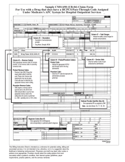


© Copyright 2026