
Statistical Analysis of data from Breast Cancer patients By Thomas Hunter Smith
Statistical Analysis of data from Breast
Cancer patients
MSc Dissertation
By Thomas Hunter Smith
School of Mathematical Sciences
University of Nottingham
I have read and understood the School and University Guidelines on plagiarism. I
confirm that this work is my own, apart from acknowledged references
Abstract
This report uses Survival Analysis techniques to analyse data on Breast Cancer patients
and attempts to determine factors which are associated with survival. Using the Nottingham Prognostic Index as a guideline and applying Kaplan-Meier, Log-Rank and Cox
Proportional Hazard Models; four main prognostic factors were identified to be directly
related to survival.
Contents
1 Introduction
1.1 Background . . . . . . . . . . . . . . . . . . . . . .
1.1.1 How did this particular project come about?
1.2 Methodology . . . . . . . . . . . . . . . . . . . . .
1.3 Results . . . . . . . . . . . . . . . . . . . . . . . . .
1.4 Breast Cancer and the NPI . . . . . . . . . . . . .
1.5 How it works..... . . . . . . . . . . . . . . . . . . . .
1.6 Geography of Breast Cancer . . . . . . . . . . . . .
1.7 The Evolution of Statistics in Medicine . . . . . . .
1.8 The Nottingham Prognostic Index . . . . . . . . . .
2 Data and Variables
2.1 Introduction to the Data . . . . . . . . .
2.1.1 A note on computing..... . . . . .
2.2 Missing Data . . . . . . . . . . . . . . .
2.2.1 Still some missing data though!! .
2.2.2 Complete Case Analysis . . . . .
2.2.3 Single Imputation . . . . . . . . .
2.2.4 Multiple Imputation . . . . . . .
2.2.5 Maximum Likelihood Estimation
2.2.6 Dealing with the missing data . .
2.3 Exploratory Analysis . . . . . . . . . . .
2.3.1 Relationships between Variables .
2.3.2 External Factors . . . . . . . . .
2.3.3 Method of Detection . . . . . . .
2.4 Summary of this Chapter . . . . . . . . .
.
.
.
.
.
.
.
.
.
.
.
.
.
.
.
.
.
.
.
.
.
.
.
.
.
.
.
.
.
.
.
.
.
.
.
.
.
.
.
.
.
.
.
.
.
.
.
.
.
.
.
.
.
.
.
.
.
.
.
.
.
.
.
.
.
.
.
.
.
.
.
.
.
.
.
.
.
.
.
.
.
.
.
.
.
.
.
.
.
.
.
.
.
.
.
.
.
.
.
.
.
.
.
.
.
.
.
.
.
.
.
.
.
.
.
.
.
.
.
.
.
.
.
.
.
.
.
.
.
.
.
.
.
.
.
.
.
.
.
.
.
.
.
.
.
.
.
.
.
.
.
.
.
.
.
.
.
.
.
.
.
.
.
.
.
.
.
.
.
.
.
.
.
.
.
.
.
.
.
.
.
.
.
.
.
.
.
.
.
.
.
.
.
.
.
.
.
.
.
.
.
.
.
.
.
.
.
.
.
.
.
.
.
.
.
.
.
.
.
.
.
.
.
.
.
.
.
.
.
.
.
.
.
.
.
.
.
.
.
.
.
.
.
.
.
.
.
.
.
.
.
.
.
.
.
.
.
.
.
.
.
.
.
.
.
.
.
.
.
.
.
.
.
.
.
.
.
.
.
.
.
.
.
.
.
.
.
.
.
.
.
.
.
.
.
.
.
.
.
.
.
.
.
.
.
.
.
.
.
.
.
.
.
.
.
.
.
.
.
.
.
.
.
.
.
.
.
.
.
.
.
.
.
.
.
.
.
.
.
.
.
.
.
.
.
.
.
.
.
.
.
.
.
.
.
.
.
.
.
.
.
.
.
.
.
.
.
.
.
6
6
6
7
7
8
9
10
10
12
.
.
.
.
.
.
.
.
.
.
.
.
.
.
19
19
20
20
21
22
22
23
24
25
29
37
38
41
43
3 Survival Analysis
44
3.1 Survival Function . . . . . . . . . . . . . . . . . . . . . . . . . . . . . . . . 45
3.2 The Hazard Function . . . . . . . . . . . . . . . . . . . . . . . . . . . . . . 46
3.3 Applications of Survival Analysis . . . . . . . . . . . . . . . . . . . . . . . 47
1
3.4
3.5
3.6
3.7
Censoring . . . . . . . . . . . . .
Purpose and Presumption . . . .
Non-parametric Survival Analysis
3.6.1 Kaplan-Meier Estimates .
3.6.2 Greenwoods formula . . .
3.6.3 Life Table Method . . . .
3.6.4 Nelson-Aalen Estimators .
Log-Rank Test . . . . . . . . . .
.
.
.
.
.
.
.
.
.
.
.
.
.
.
.
.
.
.
.
.
.
.
.
.
.
.
.
.
.
.
.
.
.
.
.
.
.
.
.
.
.
.
.
.
.
.
.
.
49
51
51
52
55
61
61
62
.
.
.
.
.
.
.
66
67
69
70
70
78
78
78
Research
. . . . . . . . . . . . . . . . . . . . . . . .
. . . . . . . . . . . . . . . . . . . . . . . .
. . . . . . . . . . . . . . . . . . . . . . . .
82
82
83
85
4 Cox Proportional Hazard Models
4.0.1 Log Likelihood test . . . . . . . . .
4.0.2 Other Methods of Model Checking
4.1 Model Building using R . . . . . . . . . .
4.1.1 Model Building . . . . . . . . . . .
4.2 Index . . . . . . . . . . . . . . . . . . . . .
4.3 Model Checking . . . . . . . . . . . . . . .
4.3.1 Schoenfeld Residuals . . . . . . . .
5 Summary, Conclusion & Further
5.1 Summary and Conclusion . . .
5.2 Further Research . . . . . . . .
5.3 Acknowledgements . . . . . . .
.
.
.
.
.
.
.
.
.
.
.
.
.
.
.
.
.
.
.
.
.
.
.
.
.
.
.
.
.
.
.
.
.
.
.
.
.
.
.
.
.
.
.
.
.
.
.
.
.
.
.
.
.
.
.
.
.
.
.
.
.
.
.
.
.
.
.
.
.
.
.
.
.
.
.
.
.
.
.
.
.
.
.
.
.
.
.
.
.
.
.
.
.
.
.
.
.
.
.
.
.
.
.
.
.
.
.
.
.
.
.
.
.
.
.
.
.
.
.
.
.
.
.
.
.
.
.
.
.
.
.
.
.
.
.
.
.
.
.
.
.
.
.
.
.
.
.
.
.
.
.
.
.
.
.
.
.
.
.
.
.
.
.
.
.
.
.
.
.
.
.
.
.
.
.
.
.
.
.
.
.
.
.
.
.
.
.
.
.
.
.
.
.
.
.
.
.
.
.
.
.
.
.
.
.
.
.
.
.
.
.
.
.
.
.
.
.
.
.
.
.
.
.
.
.
.
.
.
.
.
.
.
.
.
.
.
.
.
.
.
.
.
.
.
.
.
.
.
.
.
.
.
.
.
.
Appendices
86
A Some further Interesting findings
87
2
List of Figures
1.1
Lymphatic System . . . . . . . . . . . . . . . . . . . . . . . . . . . . . . . 13
2.1
2.2
2.3
2.4
2.5
2.6
2.7
2.8
2.9
2.10
2.11
2.12
2.13
2.14
2.15
2.16
2.17
Lymphatic System . . . . . . . . . . . . . . . . . . . . . . . . . . . . .
Estimated Survival Curves of Chemo-status amongst patients . . . . .
Scatter Plot of NPI against Survival . . . . . . . . . . . . . . . . . . . .
Scatter Plot of NPI against Survival with Fitted Survival Lines . . . . .
Scatter Plot of NPI for patients dying from Breast Cancer . . . . . . .
Scatter Plot of NPI for patients leaving the Study for Other Causes . .
Distribution of Survival for Patients Dying from Breast Cancer . . . . .
Distribution of Survival for Patients leaving the Study for Other Causes
Distribution of Survival for Patients still Alive at the end of the Study
Distribution of NPI scores across Centres (1-6) . . . . . . . . . . . . . .
Distribution of Tumour Size for Centre 1 . . . . . . . . . . . . . . . . .
Percentages of different Types of Tumour found in Centre 1 . . . . . .
Scatterplot of Tumour Size against Survival with fitted linear model . .
Histogram of age of Patients at 1st Operation . . . . . . . . . . . . . .
Histogram of age of Patients at 1st Operation . . . . . . . . . . . . . .
Distribution of Tumour Size for patients detected by screening . . . . .
Distribution of Tumour Size for patients not detected by screening . . .
3.1
3.2
3.3
Kaplan-Meier Curve computed from Table 3.6.1 . . . . . . . . . . . . . .
Kaplan-Meier Curves of Uncategorised NPI Scores . . . . . . . . . . . .
Kaplan-Meier Curves of NPI Groups with 5-year and 10-year Survival
Times . . . . . . . . . . . . . . . . . . . . . . . . . . . . . . . . . . . . .
Kaplan-Meier Curves of Tumour Size (cm) categorised into 3 groups . . .
Kaplan-Meier Curves of different types of Tumour . . . . . . . . . . . . .
Kaplan-Meier Curves for different age groups . . . . . . . . . . . . . . . .
Kaplan-Meier Curves for Endocrine Therapy . . . . . . . . . . . . . . .
Kaplan-Meier Curves for Menopausal Status . . . . . . . . . . . . . . . .
3.4
3.5
3.6
3.7
3.8
3
.
.
.
.
.
.
.
.
.
.
.
.
.
.
.
.
.
.
.
.
.
.
.
.
.
.
.
.
.
.
.
.
.
26
28
30
32
33
34
34
35
35
36
37
38
39
40
41
42
42
. 54
. 56
.
.
.
.
.
.
57
58
59
60
62
64
4.1
4.2
4.3
Kaplan-Meier Curves of Histological Grades of Tumour, as well as of the
three factors involved in calculating the grade: Pleomorphism P, MitosisM
and Tubule Formation T . . . . . . . . . . . . . . . . . . . . . . . . . . . . 71
Estimated Survival curves for 7 groups of new variable Total=T+P+M . . 72
Plots of scaled Schoenfeld residuals against transformed time for each covariate in the final CPH model . . . . . . . . . . . . . . . . . . . . . . . . . 80
A.1 Histogram of Survival for patients dying within 10 years of prognosis with
predicted survival of 85% . . . . . . . . . . . . . . . . . . . . . . . . . . . . 88
A.2 Kaplan-Meier Curves of NPI with 95% CI . . . . . . . . . . . . . . . . . . 89
A.3 Kaplan-Meier estimates of Estrogen Receptor Status . . . . . . . . . . . . 90
4
List of Tables
1.1
1.2
NPI Scores . . . . . . . . . . . . . . . . . . . . . . . . . . . . . . . . . . . . 12
Co-variates and their characteristics . . . . . . . . . . . . . . . . . . . . . . 18
2.1
2.2
2.3
Overview of the Breast Cancer Centres . . . . . . . . . . . . . . . . . . . . 21
Different Combinations of NPI . . . . . . . . . . . . . . . . . . . . . . . . . 29
NPI 5-Year Scores against actual Scores from Centre 1 . . . . . . . . . . . 30
3.1
3.2
Censoring Percentages across all centres . . . . . . . . . . . . . . . . . . . 51
Computation of Kaplan-Meier curve from section of Survival . . . . . . . . 53
.
5
Chapter 1
Introduction
”The Nottingham Prognostic Index (NPI) is an accepted prognostication tool in the management of breast Cancers. The latest overall 5-year and 10-year Breast Cancer survival
has been reported to be 85% and 77%”,
- BreastCancerResearch.com
1.1
Background
The aim of this report was to develop a thorough understanding of the branch of statistics
known as Survival Analysis and its application in Primary breast Cancer research. This
would be approached by evaluating the creation, function and application of the Nottingham Prognostic Index as well as applying methods used in Survival Analysis to a set of
data on Breast Cancer patients in an attempt to identify factors associated with survival.
1.1.1
How did this particular project come about?
Having not been particularly inspired by any of the dissertation topics kindly provided
by the University, I took it upon myself to seek an alternative subject. My passion
for medical research prompted me to look within the NHS. I managed to make contact
with Dr. Chan, a consultant at the Oncology Department at Nottingham City Hospital
and Professor Graham Ball, head Biostatistician at the John Van Geest Cancer research
centre, Nottingham. I was lucky enough to come to an arrangement which would give
me the chance to explore new statistical techniques on a real data set with information
on 16,965 Breast Cancer patients. I hope to take full advantage of this great opportunity
and deliver a final report which will include a comprehensive analysis of the data, and
perhaps include findings which may be of use in future Breast Cancer research.
6
1.2
Methodology
One of the first decisions made was to cut down the analysis to just one section of the
data which contained information on 2,203 patients. A comprehensive analysis of the
full 16,965 patients with the fluctuating inclusion and exclusion of certain co-variates and
data was unrealistic given the time frame of the report. Several different methods were
considered when dealing with the missing data, Little & Rubin (2002), including imputation and complete-case analysis - with the final consensus being that single imputation
is the most appropriate approach, implemented by an algorithm constructed in statistial
software package, R. The analysis of histograms was used to investigate distributions of
co-variates, and other visualisation techniques were used to examine the behaviour of the
data. Kaplan-Meier curves were used to compare survival times amongst the different
outcomes of a variable and the existence of significant differences between groups was
tested using log-rank. Proportional Hazard Models, Cox & Oakes (1982), were used to
identify which factors are significant in predicting a patients survival. Model checking
techniques included the Log-Liklihood ratio test, Kendall (1973), and the use of residuals,
Schoenfeld (1981) to identify violation of Proportional Hazards.
1.3
Results
Following the analysis, four prognostic factors remained significant in determining survival: Tumour Size, Histological Grade, Lymph Nodes (all of which make up the original
prognostic index) and Lymphovascular Invasion (LVI). Lymph Node involvement was
deemed to be the most important factor in determining prognosis for Breast Cancer. Despite prior thoughts to the contrary, this report found that a patients menopausal status
remains an insignificant factor, as was proven through both the log-rank test and Proportional Hazard models. The same was also true for age, although a re-categorised age
variable hinted there is evidence to suggest that these factors are not entirely insignificant
in determining prognosis. Time dependent factors such as recurrence and metastasis were
influential in determining survival, but were not considered while generating a Prognostic
Index using Proportional Hazard models, as they are unlikely to be present as prognostic
factors at the time of diagnosis. The same can be said of therapy variables. The presence
of a certain type of therapy on an individual is dictated by the biology of the tumour, thus
a patient’s survival chances must also be dictated through the biology of tumour. Rather
this than a patient’s prognosis being based on a set of information which is based on
another set of information, potentially leading to bias, loss of information and confusion.
It appears that the methods which are used to measure tumour size aren’t always fully
accurate. While measurements were being made to the nearest millimetre, an unusual
number of measurements were rounded to the nearest 0.5 of a centimetre. While this
7
rounding is for the most part compensated by the rescaling of tumour size in the Nottingham Prognostic Index, it did not fully remove the inevitability that on occasion there will
be rounding which will effect the prognostic index in a way that will alter the predicted
survival of a patient. Amongst the most significant findings was that a patient was up
to 20% more likely to survive from Breast Cancer if they have regular screening than if
they don’t. The 10 different types of tumour which existed, within the set of patients
analysed, did not prove to be an important factor in survival, although a patient with
Tumour Type 1 seemed to have smaller survival % than a patient with one of the other
nine types.
1.4
Breast Cancer and the NPI
”It is already the top Cancer in women both in the developed and the developing world,and
in many countries, it’s becoming more common.”,
World Health Organization, 2011
Breast Cancer makes up almost 1/5 of all Cancers found in women. In 2010, in the UK
alone, over 11,000 women lost their lives as a result of invasive Breast Cancer. As such, the
UK government continues to invest millions of pounds each year to aid and contribute to
various different areas of research, which share the common goal of prolonging a diagnosed
patient’s life for as long, and as pain free, as possible. Statistics is one of these areas.
• In 2010, 49,564 women and 397 men in the UK were diagnosed with invasive Breast
Cancer.
• In 2010 there were 11,633 deaths from invasive Breast Cancer in the UK.
• The most common symptom of Breast Cancer in men is a hard, painless lump that
develops on one of the breasts.
• In 2005-2009, 85 percent of women in England survived their invasive Breast Cancer
for five years or more.
• Breast Cancer is often thought of as only affecting women. Men can also develop
it, although it’s much less common. It affects just one in every 100,000 men in
England.
• In 2010, 5,765 women and 26 men in the UK were diagnosed with non-invasive
Breast Cancer.
8
1.5
How it works.....
Everybody is well aware of Cancer and the devastating effects it can have on people and
their lives, but surprisingly little people know HOW the Cancer can become fatal. In
tumours that grow inside of some vital organs, the very presence of the tumour itself
can interfere enough with the organ’s function that it eventually imparts lethal effects on
that organ. A good example of this would be a brain tumour. A brain tumour causes
tremendous amounts of localised swelling and it doesn’t have to be a large thing in order
to begin to crush vital brain tissue, leading to coma and death. Tumours of the lung can
plug off airways in a manner that leads to respiratory compromise, failure, and then death.
Cancers of the colon can obstruct the intestine or perforate, and both of these problems
can be fatal to the patient. Some tumours that arise from hormone secreting tissue such
as the adrenal glands or thyroid can actually cause such a great release of hormones that
it overwhelms the patient, leading to a fatal state. Tumour growth requires a tremendous
amount of bodily energy expenditure. This is fast growing tissue and, as a result, uses
up all of the normal energy stores and building blocks for healthy tissue such as protein.
Cancer risk increases with age:
Most Cancers are caused by DNA damage that accumulates over a person’s lifetime. Cancers that are directly caused by specific genetic faults inherited from a parent are rare. But
we all have subtle variations in our genes that may increase or reduce our risk of cancer
by a small amount - World Health Organisation
Breast Cancer, isn’t going to cause death due to the presence of the tumour in the breast
because the breast isn’t a vital organ. Breast Cancer can mestastasize to other organs
such as the liver and cause enough local destruction there to kill by way of organ damage, but even this is rare. Breast Cancer most often kills by spreading to many sites
in the body and creating enough tumour burden so that the patient is physiologically
overwhelmed, and they become cachectic and are susceptible to secondary illnesses such
as infections which ultimately lead to their demise. As the total mass of cancerous tissue
spreads throughout and the body accumulates multiple kilograms, it doesn’t matter if
it’s interfering with specific organ functions any more. The tumour burden itself starts
to make the patient ill. They begin to waste away. At that point, it’s a lot like having
AIDS or other such devastating diseases. The body becomes unable to combat even the
most minor illnesses it becomes exposed to. In these cases, patients succumb to secondary
processes like pneumonia or other infections. Not an experience that I would wish upon
anybody. So there are several different ways in which a Breast Cancer can develop and
harm the body.
9
1.6
Geography of Breast Cancer
There are surprisingly large differences in the incidence of Breast Cancer across different
parts of the world. Belgium has the highest rates at 109 out of 100,000 people (0.109%),
with other developed countries such as Australia with a 0.084% incidence rate. Compare
these to developing countries such as India (0.023%) and Mongolia which has as little
as 8 people per 100,000 diagnosed. No one has an answer to why this is the case one
train of thought is that women have children and begin breast feeding at an earlier age in
developing countries which is thought to reduce a womens chances of developing breast
cancer. But this still does not explain relatively large variations amongst countries where
the average age a women gives birth are very similar; Lifestyle, inheritance patterns, there
are many potential reasons. On the other hand, recovery rates are higher in developed
countries. ”Breast Cancer survival rates [range] from 80% or over in North America,
Sweden and Japan to around 60% in middle-income countries and below 40% in lowincome countries,” according to the WHO. The aim of this report is to draw upon the
medical data taken from 16,000 patients diagnosed with breast cancer and, through the
use of Survival Analysis and Proportional Hazard models, construct a model which will
accurately model a patients 5-year survival score. This is created with the intention
of providing the patient with as much accurate information as possible regarding their
Cancer, to help them decide upon the best course of action for themselves. There does,
of course, already exist a model which does exactly this.
1.7
The Evolution of Statistics in Medicine
It wasnt until around the 17th century that statistics was used in medicine. The idea of
statistical analysis itself was a relatively fresh and emerging concept. And indeed its use
in medicine would continuously breathe new life into medical research up right up until
the present day.
Prior to this very successful marriage, both concepts had lived very different lives.
Statistics had only really been around for a couple hundred years, while medicine itself
has been a primal instinct of humans ever since the dawn of civilisation. Prehistoric man
treated illness as a spiritual event, and would perform a whole manner of ritualistic methods to try and remove these demons. Popular techniques included Trephination (piercing
holes on the skull to ventilate these spirits) and the application of herbal medicines. For
some reason the former of these has fallen out of favour with most modern healthcare
systems, while the latter has proved more popular, and is still widely used in areas such
as Homeopathy. The evolution of medical practises was specific to the part of world it
orginated, with Europe, China, India and Native America all having their own remedies
to medical issues. It was not until the introduction of Medical Schools that medicine
really began to develop as a science, the first one of these is claimed to have been in
10
Salerno, Italy in the 13th Century. This allowed brilliant minds to work together, and
the renaissance led to revolutionary changes in the theory of medicine. In the fteenth
century, Vesalius repudiated Galens incorrect anatomical theories and Paracelsus advocated the use of chemicals instead of vegetable medicines. From the sixteenth-century
development of the microscope by Janssen and Galileo to the seventeenth century theory
of the circulation of blood (Harvey), scientists learned about the actual functioning of the
human body. The eighteenth century saw the development of modern medicines with the
isolation of foxglove (digitalis) by Withering, the use of inoculation (against smallpox) by
Jenner, and the postulation of the existence of vitamins (vitamin C, antiscorbutic factor)
by Lind.
Our knowledge (or indeed the invention and development) of Statistics on the other hand,
endured a far slower and less eventful growth spiral. Of course medical care has always
been an important part of our existence, but up until a few hundred years ago no-one
would have thought that mathematical theory could be used to help sustain and improve
human life. One of the birth places of statistics and probability was said to have been
born around 300AD when ancient greeks wanted to describe the outcome of a game of
dice between Zeus, Hades and Poseidon. Its theory developed through to the 13th century with the book of Abacus by Fibonacci and the 15th century with Luca Pacccioli
with his basic principles of probability. Cardano, Galileo, Pascal, Fermat, Bernoulli (and
his nephew) and Gataker all had significant inputs. These ideas were further refined by
scientists including Huygens (1657), Leibniz (1662), and Englishman John Graunt (1660)
wrote further on norms of statistics, including the relation of personal choice and judgment to statistical probability. Graunt in particular provided some of the first evidence
of Statistics being employed in medicine when he categorized the cause of death of the
London populace using statistical sampling. James Lind, a Royal Navy surgeon, carried
out the rst recorded clinical trial in 1747. In looking for a cure for scurvy, he fed sailors
aficted with scurvy six different treatments and determined that a factor in limes and oranges (subsequently found to be vitamin C) cured the disease while other foods did not.
His study was not blinded, but as a result (although not for 40 years)limes were stocked
on all ships of the Royal Navy, and scurvy among sailors (limeys) became a problem of the
past. By the 19th century medical research received a boom with the fast development
of technology to aid the understanding of the human anatomy. This gave birth to Case
studies which would use statistics to prove whether or not a treatment was beneficial.
Most research done before the twentieth century was more anecdotal than systematic,
consisting of descriptions of patients or pathological ndings. Many if not most of the
Statistical tests which we are familiar with today were established in the 20th century
by Sir Ronald Fisher, Archie Cochrane and Austin Bradford Hill, the first of whom is
considered by many to be the father of modern statistics. Epidemiological studies and
statistical modelling became increasingly popular, and lead to continued advancements
11
such as accelerated time failure and proportional hazard models. Statistics developed
for the purposes of medical research became commonplace across medicine, including of
course, Cancer research.
The publication by J. Mayer (2002) has a particularly fascinating take on the evolution
of medicine and statistics.
1.8
The Nottingham Prognostic Index
The Nottingham Prognostic Index (NPI) is used to determine prognosis following surgery
for Breast Cancer. Its value is calculated using three pathological criteria: the size of the
lesion; the number of involved lymph nodes; and the grade of the tumour. The formula
is shown in(1.1)
NPI = N + G + {0.2 × S}
(1.1)
Where:
• S is the size of the index lesion in centimetres (ie the Size of the Tumour)
• N is the number of lymph nodes involved: 0 = 1, 1 − 3 = 2, > 3 = 3
• G is the grade of tumour: Grade I =1, Grade II =2, Grade III =3
The resulting scores from this formula are then divided up into scores which would determine a patients predicted 5-year survival score. These scores are displayed in Table 1.8
These scores would be taken in to account when determining the patients prognosis, and
Score
5-Year Survival (%)
≥ 2.0 to ≤ 2.4
> 2.4 to ≤ 3.4
> 3.4 to ≤ 5.4
> 5.4
93
85
70
50
Table 1.1: NPI Scores
provide them with accurate information on their cancer, and their survival prospects.
The Nottingham Prognostic Index was originally derived from clinico-pathological correlation of a large series of symptomatic Breast Cancer patients. It is likely that it will need
to be revised in the near future to allow its effective application to screening patients.
- Breast Pathology on the Web
12
4
NPI
5
6
7
Figure 1.1: Lymphatic System
●
●●
●
●
●
●
●● ●
● ● ●
●
●●
●
●
●●●●● ●
●
●
●
●
●
● ● ●● ●
●
● ●
●
●●●
●●
●
●● ●●● ●
● ●
●● ●
●
●
●
●
●
●
●
●● ●
●
●
● ●
●
●
●
● ● ●●●
●
● ●
●
●
●
● ●●●
●●
● ●
●
●
●
●
●
●● ●●●
● ●● ●
●
●
●
●
●
●
●
●
●
●
●
●
● ●●
● ●●
●●
● ● ●
●
●
● ●
●●
●
●●●
●●
●●●
●● ●
●
● ●●
●●●●
●
●●
●
●
●
● ● ●
●●
● ●●●●●●
●● ●●●●●
●
●
●●
● ●
●●● ●●
● ●
●
●●● ● ●
●●
●
● ● ●
●●
●
●
●
●
●
●
●
●
●
●● ● ●● ● ● ●●●
● ●
●
●●●●●
●●●●● ●
●
● ●●
●
● ●● ●
●
●
●
●
●
●●
●
●●●●
● ●● ●●● ●●●● ●
●
●● ● ●●
● ●
●
●
●
●
●
●
●
●●
●
●●
●●●
●
●●
●●● ●
● ●● ●●
●●●●●
●
●●
●
●
●
●
●
●●
●
●
●●
●●
●
●●●
●●
●
●●●●●
●● ●
●
●●● ● ● ● ● ●
● ● ●
●●
●●●●
●● ●●
●
●
●●
● ●● ●
●
●
●
● ●
●
●
●
●
●
3
●
●
●●●●
●●
●
●
●
● ●
●
●
2
●
0
●
●
● ●
●
●
● ●
●●
50
●
●
●●
●
●●
●
●
●
● ●●
●
●
●●●
●
●
● ● ●●
●
●
●
●
●
●
●
●●
●
●●● ●
●
● ● ●● ●
●
●
●
●
100
150
●● ● ●
200
Survival (months)
Originally formulated over 30 years ago, many Cancer centres across the world have used
the above 5-year survival score derived from the NPI as one of their primary sources to
determine prognosis following surgery. While this index has proved very successful over
the years in terms of pairing up a patient to the correct surgery, scientists and statisticians
are unanimous in their opinion that there is plenty of room for improvement. An example
of such an updated version would be the development of NPI+; a new updated version
of the old index. One fact which is widely accepted across all prognostic index’s is that
the most important factor in determining prognosis is the patients Lymph Node Status.
This status is based on the number of nodes from the lymphatic system involved in the
tumour (pictured) While this revised index is considered by most to be a more proficient
at prescribing the correct surgery, there is, as always, continued room for improvement.
While conducting research for this report, many online forums were encountered regarding
the correct prognostic index, with many sufferers received contrasting answers from different places. It seems that there are still large variations in the methods used to determine
prognosis out there, even with in the UK. Unfortunately, no unique and widely accepted
method has been established and this leads to a great deal of worry across women diagnosed with Breast Cancer. This uncertainty could be detrimental to patients chances of
13
survival due to the delays it will cause in their choice of treatment. It seems ridiculous,
but this amount of disparity draws comparisons to the inconsistencies of prehistoric medical practise mentioned earlier.
Hopefully one day, our improved knowledge of the biology of Breast Cancer and the advancement of ever more sophisticated statistical techniques will see a Unified Prognostic
Index developed which will optimise a patients survival time. The best way of understanding mathematical function is to see it in action, so let us have look at some example
of a patients Nottingham Prognostic Index taken from our study:
Patient ID 4231 had a size of 2.1cm, a histological grade of 3 and no Lymph nodes involved. The simple calculation of 0.2 × 2.1 + 1 + 3 yields a prognostic index of 4.42. From
the index, this provides a an estimated 5-year survival score of 70%. This would have provided the patient and the NHS with valuable information to aid them when deciding the
next best approach for treating the Cancer. As the 5-year survival score was relatively
middle ground in relation with other NPI scores, there might have been some difficult
choices with regards to the kind of therapy to go with. As it turned out, the patient
underwent Radio Therapy and was still alive at the age of 60, almost 9 and a half years
after the Prognostic Index was assigned. This is an example of the NPI working well;
the score would have suggested a relatively intensive treatment to maximise the patients
survival, and it paid off.
Patient ID 4612 had a tumour size of 4.8cm, 4 lymph nodes involved and a histological
grade of 3, yielding a very high prognostic index of 6.96. This comprehensively gave the
patient a 5-year survival score of 50 percent. This would mean that the patient would
require chemotherapy or run a high risk of not surviving more than 5 years. This index
score once again worked well, as the poor prognosis it administered prompted the patient
to go ahead with chemotherapy and was still alive 7 and a half years after the study began
at the age of 65.
Patient ID 2271 was looking in reasonably good shape at the beginning of the study and
was assigned a Prognostic Index score of 4.4, which is equivalent (according to the NPI)
to a 5-year survival score of 70 percent. The patient was told she stood a good chance
of living past 5 years, and could perhaps decide against undergoing chemotherapy. As
a result, the patient did not undergo any kind of chemotherapy treatment and unfortunately died at 58 only 3 years after the prognosis. This is an example of the Index going
wrong the patient may well have been misled with her prognosis and skipped therapy
which while being severe, may well have saved her life.
The final patient (ID 2758) provides an example that the Nottingham Prognostic Index
was used by the patient to make a concious decision about how to proceed. In the three
examples above patients were not forced into any kind of therapy assigned from the NPI,
14
the index merely provides them with information on their chances of survival and recommends them with an appropriate plan of action which will hopefully prologue their lives
for as long as possible. This particular patient was given a very poor prognosis with an
index score of 6.9, rating their 5-year survival at 50% or less. This NPI score would normally imply a patient undergoes Chemotherapy. But on this occasion data suggests the
patient weighed up the options and decided to stay away from the very undesirable effects
of chemotherapy and live out the rest of her live in as stress free a manner as possible.
She ended up dying 3 years later at the age of 41. These moral issues are very hard to
comprehend at the best of times, let alone attempting to explain them using mathematics.
So this report shall for the main part focus away from these delicate matters and focus
on delivering a prognostic index which will give the patient as much accurate information
as possible and make their choices based on well-grounded, truthful medical evidence.
Many more patients would need to be run through the NPI to develop a good idea of how
well the index works, but already its usefulness is evident. The application of the index,
and its effectiveness will be looked at in greater detail later on.
The process of constructing a prognostic index is an arduous one. First and foremost
the statistician would be looking for as large and complete a data set as possible, and of
course with the appropriate information. Information on the age of the patient at first
diagnosis and their current status (living or dead) is simply not enough. In the case of
this analysis, as much information on the biological and surgical status of each patient is
essential. The current Nottingham prognostic index considers only 3 factors associated
with Breast Cancer, but it has long been known that it can be improved, most likely with
the addition information from other areas. The dataset analysed in this study ticked most
of these boxes: It had information on more than 16,000 patients suffering from invasive
Breast Cancer. There did, inevitably exist sections of missing data, but nothing that
could not be managed. There was information on all biological factors suspected to relate
to breast cancer as well as information on all of the surgery and therapy the patients
went through. The information was taken over a set period of time, so the patients would
not be monitored until death but only to the end of the study. It is wholly unfeasible to
conduct this level of monitoring over a long period of time for more than a few patients.
Thankfully there are techniques available to deal with this. With the exception of a few
small cases of missing, there is as much information as one could hope for at this stage.
In addition to these are Time Dependent Variables: Distant Metastases, Local Recurrence, Contralateral Breast Cancer and Regional Recurrence. These were omitted from
the Model building process, the reason for which shall be explained later. With all of
this information at hand the analysis could begin. This would roughly follow the process
displayed below:
15
1. Conduct a thorough exploratory analysis of the data. Through the use of graphical
analysis and statistical tests, develop a thorough understanding of the co-variates
and their behaviour eg. using tests to determine significance and histograms to
understand distributions
2. Once the basic knowledge of the data has been established, begin to explore intereactions and correlations within the data set, which will provide useful information
for later on when constructing a statistical model. Pearson correlation,chi-squared
test
3. Use appropriate techniques to solve the problems regarding missing data, these techniques are context dependent but the main aim is to maintain as much of the data
as possible while minimizing the bias in the process
4. Begin applying survival analysis to the data, such as calculating and plotting KaplanMeier curves, to understand differences in survival amongst variables and their outcomes Begin to sub categorise variables using log ranks tests
5. Fit Cox Proportional Hazard models to the data and slowly but surely remove variables which have little to no impact on survival, and eventually have a model which
only contains variables (and any potential interactions and necessary transformations) which effect survival from breast cancer
6. Assess the validity and accuracy of the model by running new data through it, and
measure its expected outcomes against observed outcomes. Plot residuals and test
to ensure model does not not reject the assumption of proportional hazards Wald,
Likelihood and Score. Check diagnostics: for violation of assumption of proportional hazards, for influential data and for non-linearity in the relationship between
the log hazard and the co-variates
16
7. Using the coefficients from the model, construct a new prognostics index with new
5-year survival scores
In order to complete as effective an analysis as possible we must be able to weigh up all
potential factors effecting prognosis, and whenever possible, disregard any prior beliefs
which may distort potential truths which spill out from the study. It is often the case
(and indeed was the case at several points during the study) that a piece of information
pops up which completely contradicts previous inferences on the topic. More often than
not, this is a mistake on the statisticians part or perhaps a mis-collection of data. But
every so often this isn’t the case, and the findings might be very interesting and open new
windows for discovery. Data analysis should be entered with as open a mind as possible
(within reason), and should never disregard findings which lie in the face of those previous,
unless they can be categorically disproved. Employ tried and tested methods but also try
new approaches- History tells us that people have been blinded to the truth for centuries,
simply by not even questioning a long standing and respected statement. Breast Cancer
is one of the foremost areas of medical research, and is always at the tip of a biomedical
statisticians tongue. This report may not be that elusive cure but hopefully will add a
little piece to the jigsaw which scientists from all over the world are trying to complete.
17
Variable (R-code)
Description
Menopausal Status
meno
1=Pre-Menopause, 2=Post-Menopause
63% patients post menopausal
Lymph Nodes
lymphnode
1={0 Lymph Nodes Involved},
2 = {1 − 3}, 3 = {3 <}
Tumour Type
type
Nominal Categorical
10 different types
Age at first Operation
age
Range from 18-70
Mean age 54
Tumour Size(cm)
size
Continuous Variable
Range={0.1, ..., 4.9}, Mean=1.85cm
Method of Detection
detection
1=Screening 2=Other
Screening→ regular checkups
Lymphovascular Invasion
LVI
1=Cancer cells in Blood vessels
2=Not present in Blood Vessels
Tubule formation T
> 75% =1, 10 − 75% =2, < 10% =3
Mitosis M
Mitotic Count: 1=0-9,
2=10-19,3=20+
Nuclear Cells 1=Ok
2=Bad, 3=Worse
1 = {3, 4, 5}, 2 = {6, 7}
3 = {8, 9}
Indicator Variable
1=Therapy 2=No Therapy
”” ””
Pleomorphism P
Histological Grade (T+P+M)
grade
Chemotherapy
chemo
Radio Therapy
radio
Axillary Surgery
axillary
Endocrine Therapy
endo
”” ””
”” ””
Table 1.2: Co-variates and their characteristics
18
Chapter 2
Data and Variables
2.1
Introduction to the Data
The dataset provided by the NHS contains information on 16,965 women diagnosed with
Breast Cancer taken from 10 centres around the world. This data set provides a set of
information on each diagnosed patient, mainly the biological and surgical points of interest
which are considered to be relevant in this study. A brief overview of the variables and
what is going on is displayed in Table 1.8. A detailed description of these variables, in
the context of Breast Cancer is provided in the glossary towards the end of this report:
When dealing with such a large data set, it is very easy to become overwhelmed by the
sheer size of the task which lies ahead. It is very difficult to know where to start, which
way you should approach the analysis, what goals you should be aiming for, and so on.
- A thorough understanding of Survival Analysis and the Nottingham Prognostic Index
would be needed before beginning any serious analysis. Since R would be used extensively throughout the analysis, the anticipation and interpretation of its output would
be crucial. Analysis is often a trial and error game, but that is all for nothing if you
cannot tell between a meaningful result and a meaningless result
- If a dataset of this size was ever to be analysed with some useful findings under the given
time frame, some compromises would need to be made. Would a thorough analysis of
all 16000+ patients be possible? Would all of the variables be maintained ; some of
which surpassing 50 percent missingness?
- The data needed to be as complete as possible, so techniques would need to be identified to handle the missing data. Ideally these would maintain as much information as
possible without introducing any serious bias
- Efficiency in the choice of methodology, it is no use spending weeks using one technique,
then deciding that it is no good; I would need to be strategic with my selection
19
- In addition, there are never any guarantees than any real breakthroughs will come
about, so knowing when to stop is important-no research is ever pointless!
2.1.1
A note on computing.....
The analysis for this research project was conducted solely on Microsoft Excel and R,
both of which are excellent packages. In Excel, the built in package ”Data Analysis” was
used extensively for the exploratory analysis, and was very useful for summarising and
producing basic plots of the data. The R package ”survival” was used throughout the
Survival Analysis. This has many features, including inbuilt functions which can quickly
produce survival curves as well as fit and check Proportional Hazard Models.
2.2
Missing Data
It is never a massive surprise to come across missing data when dealing with large datasets
in any field; be it engineering or analytics or medicine, for whatever reason, the existence
of missing data is almost a forgone conclusion. Having considered the magnitude of the
task ahead, and the great volumes of analysis to be performed, it was decided early
on that the focus would be on just one centre. Given the time frame of this study,
a comprehensive study across all 10 centres, all of which with having vast differences
in the information provided (such as the variables described and missing data), would
realistically be infeasible. Looking at the varying information on the patients provided
across all 10 centres, it was important to choose a centre with minimal amounts of missing
data. This goes without saying, but perhaps more important consideration , would be to
choose a centre where the missing data (each one of the 10 centres had varying counts
of missing values, spread across all variables), it was insignificant enough to not distort
the analysis in any significant way. After careful consideration and preliminary analysis,
it was finally decided that the study would be focused on Centre (1). The main reasons
being as follows:
• The Number of patients was large enough for there not be any doubt over the
accuracy of the study (Which may have been an issue if, say, centre (2) was looked
at) and was digestible enough for R to handle the analysis, which again may have
been an issue if ,say, centre (9) was looked at.
• Using prior information on the variables which may play an important role in survival, centre 1 has an almost full data set, with almost complete information across
all variables considered important for the purposes of constructing an accurate and
effective CPH model
20
Centre
1
2
3
4
5
6
7
8
9
10
No. Patients
2203
1308
562
2391
1321
604
1539
1491
4136
1410
Mean NPI
4.07
3.23
3.83
3.45
3.66
3.92
3.63
3.83
3.45
4.12
Table 2.1: Overview of the Breast Cancer Centres
• The information the censoring of patients is almost complete, as a pose to most
of the other centres, where there are vast gaps in the information, which would of
course make matters a lot more complicated
2.2.1
Still some missing data though!!
One of the main reasons Centre (1) was chosen as the focal point of the study was the
relatively small ammounts of missing information it had when compared to other centres.
Survival analyses based on a data collection process which the researcher has little control
over are often plagued by problems of missing data. Deleting cases with any missing data
will result in information loss and usually results in bias, while many analytic procedures
that retain this information in some form underestimate the resulting uncertainty in
parameter estimates and other output. Despite this, there were still some gaps in the
information on many of the key variables:
• Several of the variables (eg. Parafin Block, Frozen tissue) which were monitored in
other centres were not monitored in centre (1). For the purposes of this study, these
variables shall be disregarded. In perhaps future studies, these variables can be
analysed across the other centres, and cross referenced with the results from centre
(1), to unearth their potential importance
• There some missing points in most of the remaining variables. Ideally the solution
to this problem would not involve completely removing patients with these missing
points from the study.
Several papers were covered in the search for the best approaches to handle missingness
in a survival analysis dataset. The correct/most effective approach is obviously context
dependent but Little and Rubin (2002) stood out for its clarity and general content.
21
These approaches are more applicable for higher levels of missingness, and only one of the
variables had higher than 5% missingness. So some amount of exploration into different
methods would be useful. Such an exploration would (i) undoubtedly be useful for future
data analysis, such as going on to analyse the other centres with greater chunks of information missing, (ii) provide further insight into the data itself; it is not unusual to make
interesting discoveries as bi-products of other analysis. There were 4 main approaches:
(a) Complete Case analysis (CC) (b) Single Imputation (SI) (c) Multiple Imputation (MI)
(d) Maximum Likelihood Estimation (MLE) Like almost all statistical techniques, these
have their benefits and drawbacks.
2.2.2
Complete Case Analysis
A direct approach to missing data is to exclude them. In the regression context, this
usually means complete-case analysis: excluding all units for which the outcome or any
of the inputs are missing. There are a few different ways to do this; list wise deletion (an
entire patient would be removed from the study if they had any missing data points) and
pairwise deletion ( the patient would be removed if there were data missing from any of
the variables used in the study). Immediately these strike as nave solutions for a study
with as many covariates as this. Generally speaking, there are two main problems arise
with complete-case analysis:
1. If the units with missing values dier systematically from the completely observed
cases, this could bias the complete-case analysis
2. If many variables are included in a model, there may be very few complete cases, so
that most of the data would be discarded for the sake of a simple analysis
The small amount of missing values are well spread across the data, and the application
of CC would see almost 11 % of patients being removed from the study, so this approach
has not been deemed viable.
2.2.3
Single Imputation
Albeit a relatively simple approach, single imputation is a very easy and efficient way to
replace missing values in a data set. Once again there are several paths one can go down
with this methodology:
1. Matching: This involves identifying a variable which correlates well with the one
with missing points, and comparing data points, so for example we know that
menopausal status has a strong relationship with age so a missing value in either
could be inferred from the other
22
2. Hot-deck imputation involves sorting a dataset according to any of a number of
variables, thus creating an ordered dataset. The technique then finds the first missing value and uses the cell value immediately prior to the data that are missing to
impute the missing value. Another method is known as cold-deck imputation, which
substitutes a value (with similar correlations) taken from another cold dataset of
the same nature
3. Rth nearest neighbour: a similar approach to matching and is essentially an algorithm for imputing missing data. Rather than comparing variables of single observations, it looks at numerous observations to conjure a value to impute. This is very
useful when looking at genetic arrays where there are 10s of thousands of missing
points
4. Mean substitution: substitutes the mean of the known data of the variable for the
missing data
A consideration for these methods is dealing with categorical data such as deciding which
value to take when that calculated lies in between the categories. For example when testing
mean substitution on the variable Did the patient receive Endocrine Therapy? the mean
value from the known data was 1.57 (1=Yes, 2=No) so how would we decide which answer
to give to the 52 patients with no information? Around 80% of the variables in the dataset
are indicator or categorical, so this is of obvious concern. In addition, mean imputation
ruins the correlations among variables because it changes the way two variables co-vary.
That is, if two variables move in tandem then using mean imputation to fill in the missing
values destroys the natural relationship between the predictor and outcome variables since
the imputed values will all be the mean of the predictor and remains static for all missing
values while the outcome still varies independently.
2.2.4
Multiple Imputation
Becoming increasingly popular with the continued development of computing power, multiple imputation methods are the most popular and generally most effective method of
dealing with missing data. In order to deal with the problem of increased noise due to imputation, Rubin and Little(1987) developed a method for averaging the outcomes across
multiple imputed data sets to account for this. The way this works is that imputation
processes similar to stochastic regression are run on the same data set multiple times and
the imputed data sets are saved for later analysis. Each imputed data set is analyzed
separately and the results are averaged except for the standard error term (SE). The SE
is constructed by the within variance of each data set as well as the variance between
imputed items on each data set. These two variances are added together and the square
23
root of them determines the SE, thus the noise due to imputation as well as the residual
variance are introduced to the regression model.
*statistical noise is a term that refers to the unexplained variation or randomness that is
found within a given data sample or formula
There are many, many different techniques when implementing multiple imputation, sometimes they can be tailored to suit a set of data exclusively and sometimes they can be
used across a whole range of datasets. Below are a few examples:
(i) multiple imputation without inclusion of the outcome (MI-)
(ii) multiple imputation with inclusion of the outcome (MI+)
(iii) Multiple Imputation using regression switching with predictive mean matching
(MICE)
(iv) multiple imputation using regression switching with predictive mean matching (MICE
PMM)
(v) multiple imputation using flexible additive imputation models
2.2.5
Maximum Likelihood Estimation
Maximum likelihood involves the estimation of parameters based on the observed data
using Bayesian estimation techniques. So MLE can use information already known about
a dataset, and use that to estimate a parameter of interest, say missing data. A likelihood function is the probability or probability density for the occurrence of a sample
configuration x0 , x1 , ..., xn given that the probability density f (x | θ) with parameter θ is
known.
L(θ | x) = f (x1 | θ)f (x2 | θ); ...f (xn | θ)
n
Y
=
f (xi | θ)
(2.1)
i=0
The Maximum Likelihood Estimator (MLE) θˆ can be obtained by maximising L(θ | x) as
a function of θ. As such it is usually far more convenient to work with the log-likelihood:
l(θ | x) = logL(θ | x)
n
1X
f (xi ; θ)
=
n i=1
(2.2)
∂
ˆ There are also more developed methods
l(θ; x) = 0 To obtain a value for θ.
Then set
∂θ
which use iterative procedures for parameter estimation, namely the E-M Algorithm.
24
The iterations alternate between performing an expectation (E) step, which creates a
function for the expectation of the log-likelihood evaluated using the current estimate for
the parameters, and a maximization (M) step, which computes parameters maximizing
the expected log-likelihood found on the E step. The ebook by Millar (2011) gives a more
modern take of MLE and how it has evolved along with computing.
Maximum likelihood estimation is equivalent to multiple imputation in most cases though
maximum likelihood is easier to implement than multiple imputation thus usually more
preferred, but multiple imputation has slightly more situations in which it is applicable.
2.2.6
Dealing with the missing data
Having already disregarded Complete Case analysis, the choice remained between single
and multiple imputation. When necessary, multiple imputation can be very effective but
it can also be very complicated. It was decided that in this instance it was not necessary,
as all but one of the variables are less than 5 % missingness. Any potential extra bias
which would be brought on by using single imputation will be minimal, and would not
effect the outcome and accuracy of the analysis.
In the Endocrine therapy example mentioned above, rather than replace the 52 missing
values with the value 2 as the average was 1.57, a function in R was used to randomly
insert the values based on the values already taken for this variable. So in this example the
random.impfunction randomly inserted 32Nos and 20 Yess into the missing data points.
random.imp <- function (a){
missing <- is.na(a)
n.missing <- sum(missing)
a.obs <- a[!missing]
imputed <- a
imputed[missing] <- sample (a.obs, n.missing, replace=TRUE)
return (imputed)
}
This algorithm worked extremely well for the majority of variables missing points, however there were a few which required more attention:
Internal Mammary Nodes
Of the 1564 patients accounted for in this variable, 98.15% 0 Internal Mammary Nodes,
with 1.66 % having 1 and 0.29 % having 2. With around 30 % missing, this was the variable had by far the most missing information (with all others being less than 5 percent
25
Figure 2.1: Lymphatic System
700
120.00%
600
100.00%
500
# of Patients
80.00%
400
60.00%
300
40.00%
200
20.00%
100
0
0.00%
3
4
5
6
7
8
9
More
T+P+M
missingness), imputing new values would be a relatively arduous task. With this being the
only variable with substantial missing information, conditions are ideal for non response
weighting to be applied. This would be a long and relatively fruitless task, considering
the fact that it correlates strongly with number of Axillary nodes positive. Due to this
high level of correlation, the decision was made to
Tubile Formation, Pleomorphism and Mitosis
These three factors are used to calculate the final Histological Grade of the tumour.
Twenty five patients had all three of these missing at once, and a further 5 had just Mitosis
missing. Fortunately, every single patient had their final histological grade, so it wasn’t
difficult to impute values such that they didn’t violate the criteria. For example, one
patient had information on the final grade, as well as Tubile formation and Pleomorphism
both being graded 3. The histological grade was 2, so the only value Mitosis could
take would be 1, otherwise there would be inconsistency in the model. The sub grade
information for T, M, P for those patients with all three missing was imputed under the
assumption that:
• those with a histological grade of three would automatically have a grade of 3 for
Tubile formation and Pleomorphism
26
• those with a histological grade of one would automatically have a grade of 1 for
Mitosis and Pleomorphism
Having manually filled in the points to match this criterion, the random.imp function
could be used to randomly insert the rest of the missing data for T,P and M.
Recurrence
The problem with these recurrence variables is that their potentially hazardous effects
don’t usually become present until some time after the patient has had initial surgery.
This means recurrence is a time-dependent covariate, which has the potential to make
the model building process far more complex. It is clear from the data that the recurrence variables have a large say in the patient’s survival, so it is important that they are
taken into account when modelling survival. Unfortunately the fact that they remain
anonymous until sometime until after the patient’s first prognosis means that they will
essentially be useless in a Prognostic Index as it is unlikely that any sign of them will
appear until some months and years after the patients first 5-year survival score is given.
There does exist methods which accommodate Time dependent variables into a model,
but in this situation they are not required: while it will be possible how the existence
of recurrence effects survival, it is unlikely that a model will exist which can accurately
predict if recurrence will occur. As such the time dependent variables which involve recurrence were removed from the study.
Chemotherapy and the 9s....
An interesting problem arose when it was unveiled that 59 (2.7%) patients had observation
which contained 9s in place of where the standard 1’s and 0s would be for Chemotherapy.
Figure 2.2 shows that this third outcome has even lower survival times than those who
underwent chemotherapy. One possible answer to this is that patients who had this outcome did undergo chemotherapy, but ceased the treatment as their cancer had developed
to a point that survival seemed unlikely. The choice was made to keep these data points as
they are, and treat chemotherapy as an ordinal categorical variable. This decision makes
sense in that there is a clear difference in the survival times for these three outcomes.
Later research using the log-rank test confirmed a clear separation in survival between
the three outcomes.
Summing up this section, there was a substantial amount of lists and a,b,c-ing which
explains the great variety of methods which exist for handling missing data. As was
mentioned earlier, the right approach is always context dependent but, even in matters
regarding a single issue there are often several approaches to take. Another major con27
0.2
0.4
^
S(t)
0.6
0.8
1.0
Figure 2.2: Estimated Survival Curves of Chemo-status amongst patients
0.0
Chemotherapy
No Chemotherapy
Unknown Therapy
0
50
100
150
t
28
200
sideration are the time restraints put in place. In the case of this report the choice of
approach was not complicated by this factor due to the low levels of missingness which
required only the simple matter of single imputation. The application of methods of multiple (regression based )imputation would probably have resulted in reduced biased, but
give the low levels of missing data and the given time restraints, single imputation was
deemed adequate.
2.3
Exploratory Analysis
A long time was spent exploring variables, their relationships with each other, distributions and effect on survival. Considering the behaviour of the original NPI against
survival provided a reasonably good starting point. We can see that the prognostic index
scores are segregated into five clear groups, which makes good sense if we break down the
combinations of the score in Table (2.3). S = 0.2×Tumour Size ≈ 0.36 ± 0.12, based on
the median values for tumour size, is assumed be consistent for each combination.
This is reflected in Figure 2.3, with the patients clustered around the NPI regions of
Group
(1)
(2)
(2)
(3)
(3)
(3)
(4)
(4)
(5)
Lymph Node Status
1
1
2
2
3
1
3
2
3
Histological Grade
NPI Score
1
≈ 2.36 ± 0.12
2
≈ 3.36 ± 0.12
1
”” ””
2
≈ 4.36 ± 0.12
1
3
”” ””
2
≈ 5.36 ± 0.12
3
”” ””
3
≈ 6.36 ± 0.12
”” ””
Table 2.2: Different Combinations of NPI
(2.24,2.48), (3.24,3.48), (4.24,4.48),(5.24.,5.48),(6.24,6.48) and is even more evident in
the distribution of the NPI scores in Figure2.10. The size of these regions is down to
the first and third Quartiles of Size multiplied by the 0.2 as noted in the index. The
data points lying outside of these regions were patients with either exceptionally small or
exceptionally large tumour sizes.
The majority of the observations lie in the groups (2) and (3) of the index. What may
be of interest now, and potentially useful for looking at constructing a new index later
on is to see how these five groups differ in survival. For groups (1) and (2), the majority
29
4
2
3
NPI
5
6
7
Figure 2.3: Scatter Plot of NPI against Survival
●●● ●
●
●●
●●
●
●
●●
● ● ●
●
●
●●
●
●●●
●
●
●●
●● ●
●
●●
●
●
●
●
●
●●
●
●
●
●
●
●
●●●●● ●
●
●
●● ●
●
●
● ●
●
●
●
●
●
●● ●●● ●●●
●
●
●
●● ●
●
●●
● ● ●●
●●● ●
●
●
●
●
●
●
●
●
● ●● ●●
●
●
●●
●●
●
●
●
● ● ●●● ● ●●
● ●●
●● ●
●●
● ●●● ● ●
●●●
●●
● ●●●●
●●
●
● ●
●●●
●●
●
●● ●●
●●
●●
●●●●●
● ● ●● ●
●
●
●
●
●
●
●
●
●
●
●
●
●
●
●
●
●
●
●
●
●
●
●
●
●
●
●
●
●
●
●●
●
●● ●●● ●
●●
●● ●●
● ●
●●●
●●
●●
●●
●●
●●●
●
●
●
●● ● ●●
●●●
● ●●● ●
●● ●
●
●
●
●
●●●
●
●
●●
●
●●
●
●
●
●
●●
●●
●
●
●
●●
●
● ●
●●●
●●●
●
●●●● ●●
●
●
●
●●
●● ●
● ●●
●●●
●●
●●●●
●●●
●
●
●
●●●
●
●
●●
●
●
●
● ● ●●
●
●●●
●
●
●
●●
●
●
● ●●●
●●
●●
●●
●
●●
●●
●●●
●
●
●
●●●●
● ●
●●●
●●●●
●●
●●● ●●●●●●●
●●
●
●
●
●●●● ● ●
●
●
●
● ● ● ●● ● ●● ●●
● ●●
●●●
● ●
●●
●●●● ●● ●● ●● ●●
● ●●
●
●
●
●
●
●
●●
●●
●
●
●
●●●●
●
●● ●
●● ●
●
● ●
●
●
●
●
●
●● ●●
●● ●● ●●● ● ●● ●●
● ● ●
●●
●●
●
●
●● ●
●
●
●● ●
●
● ● ●●
●
●●
●
●●
●●●●
●
●
●
●● ●●
●
●●
●●
●
●
●●
●
●
●●
●●
●●
●●
●●
●
●●
●
● ●● ●
●
●
●
●
●●
●
● ●●
●
●
●
●
●
●
●
●
●
●
●
●
●●
●
●●
●●●
●
●
● ● ●
●
●
●
●
●
●
●●
●
●
●
●
●
●
●
●
●
●
●
●
●
●
●
●
●
●
●
●
●
●
●
●
●
●
●
●
●●●●
●●
●
●●
●
●
●
●
●
●
●
●
●
●
●
●
●
●●
●●●
●
●
●
●
●
●
●
●
●
●
●
●
●
●
●
●
●
●
●
●
●●
●●
●
●
●●●
●
●●●
●●
●
●●
●
●
●
●
●
●
●●
●●●
●
●
●
●
●
●●
●
●
●
●
●
●●
●
●●
●
●
●
●
●
●
●
●
●
●
●
●
●
●
●
●
●
●
●
●
●
●
●
●
●
●
●
●
●
●
●
●
●
●
●
●●
●
●
●●
●
●
●
●
●
●
●
●●
●
●
●●● ●
●
●
●
●
●
●●
●●
●
●
●
●
●
●
●
●● ●●●
●
●
●
●●
●
●
●
●
●
●
●
●
●
●
●
●●
●
●
●
●
●
●
●
●
●
●
●
●
●
●
●●
●
●
●
●
●
●
●
●
●
●
●
●
●
●
●
●
●
●
●
●
●
●
●
●
●
●
●
●
●
●
●
●
●
●●●
●
●
●
●
●
●
●
●
●
●
●
●
●
●
●
●
●
●
●
●
●
●
●
●
●
●
●
●
●
●
●
●
●
●
●
●
●
●
●
●
●
●
●
●
●
●
●
●
●
●
●
●
●
●
●
●
●
●
●
●
●
●
●●
●
●
●
●
●
●
●
●
●
●
●
●
●
●
●
● ●●●
●
●
●
●
●
●
●
●
●
●
●
●
●
●
●
●
●
●
●
●
●
●
●
●
●
●
●
●
●
●
●
●
●
●
●
●
●
●
●
●
●
●
●
●
●
●
●
●
●
●
●
●● ●
●
●● ●●●
● ●
●
● ● ●●
●
●●●●
●●
●
●●
●
●
●
●
●●●●
●●
●●●● ● ●
●
●
●
●
●
●
●
●
●
●
●
●
●
●
●
●
●
●
●
●
●
●
●
●
●
●
●
● ● ● ●●
● ●
●
● ●
●●●● ●
●
●
●
●
●
●
● ●● ●
●
●
● ● ● ● ●● ●●
● ●●
●
●●
●
●●
●●
● ●●
●
●
● ●●●●●
●●
●●
●●
●
●
●
●
● ●
●
●
●
●●
●●●●●
●
●
●
●
●
●●●
● ●●●
●●
●
●
●● ●
●
●
●
●
●
● ●●
●
●
●
●
●
●
●
●●
●
●●
●●●
●
●
●
●
●
●
●
●
●
●
●
●
●
●
●
●
●
●
●
●
●
●
●
●
●
●
●
●
●
●
●
●
●
●
●
●
●
●
●
●
●
●
●
●
●
●
●
●
●
●
●
●
●
●
●
●
●
●
●
●
●
●
●
●
●
●
●
●
●
●
●
●
●
●
●●
●
●
●●
●
●
●●
●
●
●●
●
●
●
●
●
●●
●●
●●
●●
●
●●
●
●
●
●
●
●
●
●●●
●●● ● ●●
● ●
●
●
●
●
●
●
●
●
●
●
●
●
●
●
●
●
●
●
●
●
●
●
●
●●
●●
●
●
●
●
●
●
●
●
●
●
●
●
●
●
●
●
●
●
●
●
●
●
●
●
●
●
●
●
●
●
●
●
●
●
●
●
●
●
●
●
●
●
●
●
●
●
●
●
●
●
●
●
●
●
●
●
●●
●
●
●
●●●
●
●
●●
●●●●●●
●
●●
●
●
●
●
●
●
●
●
●
●
●
●
●
●
●
●
●
●
●
●
●
●●
●●●
●
●
●
●
●
●
●
●
●
●
●
●
●
●
●
●
●
●
●
●
●
●
●
●
●
●
●
●
●
●
●
●
●
●
●
●
●
●
●
●
●
●
●
●
●
●
●
● ●●●
●● ● ● ●
●
● ●●● ●
●
●
●
● ●
●
●
● ● ●● ●
●
●●
●
●
●●
●●● ●
●●
●
●
●
●●
● ●
●
● ●
●
●●
●
● ●● ●●●●
●●
●
●
●
●
●
●
●
●
●
●
●
●
●
●
●
●
●
●
●
●
●
●
●
●
●●
●
●
●
●
●
●
●
●
●
●
●
●
●
●
●
●
●
●●●●
●
●
●●
●
●●●
●
●
●
●
●
●
●
●
●
●
●
●
●
●● ●●
●
●
●
●
●
●
●
●
●
●
●
●
●
●
●
●
●
●
●
●
●
●
●
●
●
●
●
●
●
●●
●
●
●
●
●
●
●
●
●
●
●
●
●
●
●
●
●
●
●
●
●
●
●
●
●
●
●
●
●
●
●●
●
●●●
●●
●
●
●
●
●
●
● ●●●●
●●
●
●●
●●
●
●●
●●
●
● ● ●
●
●
●
●
●
●
●
●
●
●
●
●
●
●
●
●
●
●
●
●
●
●
●
●
●
● ● ●
●
●
●
●
●
●
●
●
●
●
●
●
●
●
●
●
●
●
●
●
●
●
●
●
●
●
●
●
●
●
●
●
●
●
●
●
●
●
●
●
●
●
●
●
●
●
● ●●●●
●●
● ●● ●●
● ●● ●
●●
●
● ● ●●●
●
●
●●
●
●● ●
●
●
0
50
100
●
150
200
Survival (months)
of the patients had a survival time of more than 80 months, and while the same applies
for (3), there is an clear increase of patients surviving < 80 months. A measure of the
accuracy and performance of the NPI against the 2203 patients from Centre (1) can be
easily obtained. Table (2.3) shows the 4 different categories of NPI scores, the number of
patients and the actual survival percentages of each group in Centre (1).
It is immediately transparent that there are huge differences between the index score
5-Year Survival (NPI Score)
90% (≥ 2− ≤ 2.4)
85% (> 2.4− ≤ 3.4)
70% (> 3.4− ≤ 5.4)
50% (≥ 5.4)
Number of Patients
% Survival Actual
321
96.4% (307 patients)
468
95.1% (445 patients)
1107
86.2% (954 patients)
308
61% (188 patients)
Table 2.3: NPI 5-Year Scores against actual Scores from Centre 1
and the actual score - is this intentional? Looking at the different categories of 5-year
survival, these patients do not match very well with the predicted survival percentages. The lower scores (< 2.4)for the NPI matches well with insignificant difference
30
(pairedt − test, α = 0.05) however the three subsequent categories are less encouraging.
For the next two stages, the prognostic predicted survival differs significantly(α = 0.05)
with 10% and 11% difference respectively, with more patients surviving beyond the 5-year
mark than the index anticipated. And the final category anticipated 10% more people
surviving then actually did. Additionally 85% survive longer than 5 years, which emphasises how the vast majority of patients have low range NPI scores. It is initially surprising
to see that less than 50% of the patients survive for less than 10 years, but this is likely to
be a figure severely distorted by censoring, meaning that the survival times for this data
take into account patients who were still alive at the end of the study, from which point
their age cannot be monitored. Thus it that age is used for the analysis. Since many of
these studies will last less than 10 years, the true percentage survival at 10 years is tricky
to establish. The 5-year survival is far easier to clarify, as almost all studies of this nature
will last at least 5 years. So we have seen there are significant inconsistencies, and you
would expect something as developed as the NPI to be more accurate there are several
possible reasons for this.
Were possibly not enough patients tested on? There seem to be different levels of survival
across centres Centre (1) seems to have reasonably high levels
Perhaps the index is designed to be under predict survival by around 10% to make
patients think more cautiously about their choices. I would be interesting to hear the
truth, and if indeed this is the truth, is it morally right for NHS to distort information
for the patients in such a way?
Or perhaps the NPI is that inaccurate and in desperate need to revising?
Interesting thought......when counting up the patients surviving less than 5 years after diagnosis there was quite a high intensity of patients dying slightly after the 5-year
survival time, especially 6-7 years as can be seen in Figure A.1. This shows the distribution of time of death for patients with NPI score > 2.4to3.4 ≤ dying before 10 years.
This is one of a few examples where 5 years as time point of reference for survival seems
inappropriate. On this evidence, were this particular prognostic index to be used, either
the survival % for each group should be increased by 10% or the time point be increased
to 7 years. If this was to be performed to the scores from centre 1, the actual scores would
be insignificantly different (α = 0.05) to the NPI scores. Figure 2.4 demonstrates how the
predefined categories segment the data. The vertical red line represents the 5 year mark,
and the blue horizontal lines mark the different categories which determine survival. So
as we are moving upwards through the sections we are expecting the number of points on
the right to decrease and on the left to increase (in propotional terms for that particular
category). While this is the case, it does not fit in with the levels of survival stated by
the NPI. The green lines represent the actual times which would need to be assigned
to this dataset if the prognostic index was to maintain the survival percentages for its
31
4
3
2
NPI
5
6
7
Figure 2.4: Scatter Plot of NPI against Survival with Fitted Survival Lines
●●● ●
●
●●
●●
●
●
●●
●
● ● ●
●
●
●●
●
●
●
●
●
●
● ●●● ●● ●●
● ●●
●
●
●●
●
●
●
●
●
●
● ●
●● ●●
●
●
● ●
●● ●●●
●
●
● ●●
●
●
●● ●●● ●●●
●
●
●
●
●
●
●
●
●
●
●
●
●● ●●
●
●
●
●
●
●
●
●
●
● ●
●
●
●●
●●
●
●
●
● ● ●●● ● ●●
● ●●
●● ●
●●
● ●●● ● ●
●●●
●●
● ●●●● ●
●
● ●
●●●
●●
●●
●
●● ●●
●●
●
●●●
●●
●
●● ● ●●
●
●
●● ● ● ●●
●
●
●●
●●●● ● ● ●
●
●
●
●
●
●
●
●
●
●
●
●
●
●
●
●
●
●
●
●
●
●
●
●
● ●
●●
●●
●
● ●●●●●
●
●●●
●
●
●● ●
●● ● ●●
●●●
● ●
●
●
●●
●●●
●
●●
●
●●●
●
●
●
●
●●
●
●
●● ●
●●
●
●
●●
●
●
●●
●
● ●
●●●
●●●
●
●●●● ●●
●●●●
●
●●
● ●●
●●
●● ●
● ●●
●
●
●●●
●
●
●●
●
●
●
● ● ●●
●
●●
●
●●●
●
●
●
●●
●
●
●●
●●
●
●
●●
●●●
●
●
●
●●●●
● ●
●●●
●●●●
●●
●●● ●●●●●●●
●●
●●
●● ●●
●
●
●
●●●● ● ●
●●
●
●
●●
●
● ● ● ●● ● ●● ●●
●●
● ●
●●
●●●● ●● ●● ●● ●●
● ●●
●
●
● ●
● ●●
●●
●●
●
●
●
●
●
●● ●
●
●
● ●
●
●
●●●
●
●
●● ●●
●● ●● ●●● ● ●● ●●
● ●
●●
●●
●
●
●
●● ●
●
●
●● ●
●
● ● ●●
●●
●
●●
●●●●
●
●
● ●●● ●●
● ● ●●
●●●
●
●
●
●●
●
●
●●
●●
●●
●●
●●
●
●●
●
● ●● ●
●
●
●
●
●
●
●●
●
● ●●
●
●
●
●
●
●
●
●
●
●
●
●
●●●
●
●
●
●
●
●
●●
●
●●
●●
●●●●●●
●●●
●●●
●
●
●
●●●
●●
●●
●
●
●
●
●
●
●
●
●●
●
●●
●●
●
●
●●
●
●●●●
●●
●
●●
●
●
●
●
●
●
●
●
●●
●●●
●
●
●
●
●
●
●
●
●
●
●
●
●
●
●
●
●
●
●
●
●
●
●
●
●
●
●
●
●
●
●
●
●
●
●
●
●
●
●
●
●
●
●
●
●
●
●●
●
●●
●
●●
●
●
●
●
●
●
●
●
●
●
●
●●
●
●
●
●
●
●
●
●
●
●
●
●
●
●
●
●
●
●
●●
●
●
●
●●
●
●●
●
●●
●
●
●
●
●●
●
●
●●
●
●
●● ●
●
●
●
●
●●
●●
●●●
●
●
●●
●
●
●
●
●
●● ●●●
●
●
●
●●
●
●●●
●
●
●
●
●
●
●
●●
●
●
●
●●
●
●
●
●
●
●
●●
●
●●
●
●
●
●
●
●
●
●
●
●
●
●
●
●
●●
●
●
●
●
●
●
●
●
●
●
●
●
●
●
●
●
●
●
●
●
●
●
●
●
●
●
●
●
●
●
●
●
●
●
●
●
●
●
●
●
●
●
●
●
●
●
●
●
●
●
●
●
●
●
●
●
●
●
●
●
●
●
●
●
●
●
●
●
●
●
●●
●
●
●
●●
●
●
●
●
●
●
●
●
●
●
●
●●
●●● ●●●
● ●●●
●
●●
●
●
●
●
●
●
●
●
●
●
●
●
●
●
●
●
●
●
●
●
●
●
●
●
●
●
●
●
●
●
●
●
●
●
●
●
●
●
●
●
●
●
●
●
●
●●
●●● ●
●●● ●●
●
●
●
●
●
●
●
●
●
●
●
●
●
●
●
●
●
●
●
●
●
●
●
●
●● ●●
●
●
●● ●●●●●●●
●
●●
●
●
●● ●
●● ● ●
●
●
●
●
●●●
●
● ● ●●●
●
●
●
● ●●
● ●
●
●
●
●
●●●
●
● ●
●
●
●
●
● ● ●● ●●
● ●● ●
●
●
●
● ●●
●
●
●
●●
●●
● ●●
●
●
● ●●●●●
●●
●●
●
●●
●●
●
● ●
●●●
●●
●
●●
●●●●●
●
●
●
●
●
●●●
●
●● ●
●●
●
●
●● ●
●●
●
●
●
●
●
●
●
●
●
●
●●
●
●●
●
●
●
●
●
●
●●
●
●
●
●
●
●
●
●●
●
●
●
●
●
●
●
●
●
●
●
●●●
●●●
●
●
●●
●
●● ●
●●
●
●
●
●
●
●
●
●
●
●
●
●
●
●
●
●
●
●● ●● ●●
●
●
●
●
●
●
●
●
●
●
●
●
●
●
●
●
●
●
●
●
●
●
●
●
●
●
●
●
●
●
●
●
●
●●
●
●●
●
●
●
●
●
●
●
●
●
●
●
●
●●
●
●
●
●●
●
●
●●●
●
●
●●●
●
●
●
●●
●
●●
●●
●●
●●
●
●●
●
●
●
●
●
●
●
●
●
●●
●●
●●
●
●●
●
● ●● ●
●
●
●
●
●
●
●
●
●
●
●
●
●
●
●
●
●
●
●
●
●
●
●
●
●
●
●
●
●
●
●
●
●
●
●
●
●
●●
●
●
●
●
●
●
●
●
●
●
●
●
●
●
●
●
●
●
●
●
●
●
●
●
●
●
●
●
●
●
●
●
●
●●●
●
●
●●
●●●
●●
●
●
●
●
●●
●
●●●
●●●●
●●●
●●
●
●
● ●● ●
●●●●●
●
●
●
●
●
●
●
●
●
●
●
●
●
●
●
● ●●●
● ●●● ● ●
●● ● ● ●●
●
●
●
●
●
●
●
●
●● ● ●
●
●●
●
●●
● ● ● ● ● ●●
●
●
●
●
●●
●
●
●
● ●
●
●●
●
● ●● ●●●●
●●
●
●
●
●
●
● ●
●
●
●
●
●
●
●
●
●
●
●
●
●
●
●
●
●
●●
●
●
●
●
●
●
●
●
●
●
●
●
●
●
●
●
●
●
●
●
●
●
●
●
●
●
●
● ● ●●●
●
●
●●●
●
●
●
●● ●●
● ●●● ●
● ●●
●
●
●
●●
●
●
●
●
●●
●
●
●
●
●
●
●
●●●
●
●
●
●●
●
●
●●●
●●●
●
●
●
●
●
●
●
●
●
●
●
●
●
●
●
●
●
●
●
●
●
●
●
●
●
●
●
●
●
●
●
●
●
●
●
●
●
●
●
●
●
●
●
● ● ●
●●
●
●●
●
●
●
●●
●●
●●
●
●●●
●●●
●
●● ●
●
●
●
●
●●
●●●
●●●
●●
●
●●
● ●
●●
●
●
●
●
●
●
●
●
●
●
●
●
●
●
●
●
●
●
●
●
●
●
●
●
●
●
●
●
●
●
●
●
●
●
●
●
●
●
●
●
●
●
●
●
●
●
●
●
●
●
●
●
●
●●●●
●
●
● ● ● ●●
●
● ● ●● ●
●
0
50
●
100
survival
32
150
200
4
NPI
5
6
7
Figure 2.5: Scatter Plot of NPI for patients dying from Breast Cancer
●
●●
●
●
●
●
●● ●
● ● ●
●
●●
●
●
●●●●● ●
●
●
●
●
●
● ● ●● ●
●
● ●
●
●●●
●●
●
●● ●●● ●
● ●
●● ●
●
●
●
●
●
●
●
●● ●
●
●
● ●
●
●
●
● ● ●●●
●
● ●
●
●
●
● ●●●
●●
● ●
●
●
●
●
●
●● ●●●
● ●● ●
●
●
●
●
●
●
●
●
●
●
●
●
● ●●
● ●●
●●
● ● ●
●
●
● ●
●●
●
●●●
●●
●●●
●● ●
●
● ●●
●●●●
●
●●
●
●
●
● ● ●
●●
● ●●●●●●
●● ●●●●●
●
●
●●
● ●
●●● ●●
● ●
●
●●● ● ●
●●
●
● ● ●
●●
●
●
●
●
●
●
●
●
●
●● ● ●● ● ● ●●●
● ●
●
●●●●●
●●●●● ●
●
● ●●
●
● ●● ●
●
●
●
●
●
●●
●
●●●●
● ●● ●●● ●●●● ●
●
●● ● ●●
● ●
●
●
●
●
●
●
●
●●
●
●●
●●●
●
●●
●●● ●
● ●● ●●
●●●●●
●
●●
●
●
●
●
●
●●
●
●
●●
●●
●
●●●
●●
●
●●●●●
●● ●
●
●●● ● ● ● ● ●
● ● ●
●●
●●●●
●● ●●
●
●
●●
● ●● ●
●
●
●
● ●
●
●
●
●
●
3
●
●
●●●●
●●
●
●
●
● ●
●
●
2
●
0
●
●
● ●
●
●
● ●
●●
50
●
●
●●
●
●●
●
●
●
● ●●
●
●
●●●
●
●
● ● ●●
●
●
●
●
●
●
●
●●
●
●●● ●
●
● ● ●● ●
●
●
●
●
100
150
●● ● ●
200
Survival (months)
set categories. From this visual demonstration we see that we would need to squeeze or
retract the blue lines enough so that the green line matches the red line. This would
require altering the margins to something more or less than 1 (or 2), and obviously. The
nature of this obviously requires on the distribution of the points. Were they uniformly
distributed, it would be easier to see how the index would needed to be altered to fit the
data.
In the case of centre 1, the data are gathered in 5 groups, but there are only 4 categories
for these to fall into. There is no immediate explanation for this, but it is a reminder that
the model building is just part of the process, and the subsequent index requires some
amount of visualising.
Figures 2.5 and 2.6 represent the difference in NPI scores for patients dying from breast
cancer those leaving the study from other causes. These can help visualize the possibility
of informative censoring.
After looking at the age distributions for Death from Cancer in Figure (2.7), leaving the
study other causes (Figure 2.8) and still alive at the end of the study (Figure 2.9), they
all have strong suggestion that they belong to a family of normal distributions. But by
33
Figure 2.6: Scatter Plot of NPI for patients leaving the Study for Other Causes
●
● ●
●
●
6
●
●
●
● ●●
●
●
●
●
●
●
●
●●
●
●
●●
●
●
5
●
●
●
●
● ●
●
●
●
●
4
NPI
●
●●●● ●
●
● ● ●●
●
●
● ●●
●● ● ● ●
● ●
●
● ●
●
● ●
●
●
●
●● ● ●
●
3
●
●
●
● ●●
●
● ●● ●
● ● ●
●
●
●
●
●
●
●
●
● ● ●
●● ●● ●
● ●
●
●
2
●
●
0
●
●
●
●
●
●
●
●●● ●
● ●●
●
●
●
●
●
●●
● ● ●● ●
● ●
● ●
●● ● ● ●●
50
●
●
●
●
●
●
100
●
●
●
●
●
●
●
●
●●
●
●
●
●
●●●
●●
●
●
150
●
200
Survival (months)
Figure 2.7: Distribution of Survival for Patients Dying from Breast Cancer
485 patients dying of from breast cancer
40
35
Frequency
30
25
20
15
10
5
0
Age
34
Figure 2.8: Distribution of Survival for Patients leaving the Study for Other Causes
173 patients dying from other causes
25
Frequency
20
15
10
5
0
40
44
48
52
56
60
64
68
72
76
80
84 More
Age
Figure 2.9: Distribution of Survival for Patients still Alive at the end of the Study
1545 patients still alive at the end of the study
140
120
Frequency
100
80
60
40
20
0
Age
35
Figure 2.10: Distribution of NPI scores across Centres (1-6)
Distribution of Nottigham Prognostic Index Scores across
patients from Centres 1-6
800
700
Frequency
600
500
400
300
200
100
0.1
0.3
0.5
0.7
0.9
1.1
1.3
1.5
1.7
1.9
2.1
2.3
2.5
2.7
2.9
3.1
3.3
3.5
3.7
3.9
4.1
4.3
4.5
4.7
4.9
5.1
5.3
5.5
5.7
5.9
6.1
6.3
6.5
6.7
6.9
More
0
NPI
comparing these histograms, information can be gathered which may give more insight
into the nature of the censoring. The similar patterns all three groups follow follow suggest that the reasons for those who left the study for other causes, may be linked to the
breast cancer. While these deaths might not come directly from breast cancer, they may
be directly associated with it.
Spreading across other centres, Figure (2.10) looks at the NPI of over 8,000 patients. It
can be seen that the patterns of the histograms follow a similar shape to the other groups
looked at. But Immediately it is evident that something is not quite right as the graph
is displaying a number of patients with NPI scores of less than the base rate of 2. This
will be the result of either missing information on the Tumour Grade or the Number of
Lymph Nodes involved.
Looking at Figure (2.11), once again a normal distribution comes to mind. On closer
inspection it becomes evident that there is a disproportionate frequency of patients with
a Tumours Sizes with factor 0.5, implying that for more than a few patients, this measurement is being rounded up/down to the nearest factor of 0.5, which is surprising. The
histogram suggests that it is possible to accurately measure the size of a tumour to the
nearest mm, yet it is obvious that less accuracy has been used in many instances. Given
that the size of the tumour plays a relatively large role in determining prognosis, hence
the choice of surgery, hence the chances of a patients survival, perhaps more time and
36
Figure 2.11: Distribution of Tumour Size for Centre 1
Distribution of Tumour Size amongst patients in Centre 1
250
Frequency
200
150
100
50
0
0.2
0.4
0.6
0.8
1
1.2
1.4
1.6
1.8
2
2.2
2.4
2.6
2.8
3
3.2
3.4
3.6
3.8
4
4.2
4.4
4.6
4.8
5
0
Tumour Size (cm)
effort could be invested in measuring the tumour size as accurately as possible. Having
said that, the potential dangers of this measurement strategy will be limited substantially
be the fact that Tumour Size is only 20% present in the final NPI. It is quite possible that
those involved in the measurement process were well aware of this fact. Were Tumour Size
to carry more power within a Prognostic Index, perhaps there would be more emphasis on
the accuracy. Additionally it seems more accuracy is used for measuring smaller tumours
(< 1.5cm), and as the size increases, so does the amount of rounding.
There were 9 different types of tumour found in the patients. Figure (2.12) shows that
the majority are of type 1, with type 11d also making up a large share of the patients.
With such a range of tumour types, instinct dictates that differentiation between types
may influence survival in some way. A pie chart is no way to measure this but later on,
differences in survival between types will be investigated using Kaplan-Meier estimators.
2.3.1
Relationships between Variables
With the range of types of variable in the dataset, there does not exist a single generalised method to detect relationships. Since there exists continuous data (eg Survival),
nominal categorical (eg Tumour type), ordinal categorical (eg Histological Grade) as well
as binary/indicator variables (eg Endocrine therapy; a great deal of care must be taken
in choosing the correct method for each situation. A rigorous procedure of comparing
37
Figure 2.12: Percentages of different Types of Tumour found in Centre 1
% Spread of Tumour Types
T12
1.54%
Missing
0.50%
T11d
24.33%
T8
0.22%
T1
58.24%
T7
5.44%
T3
6.72%
T6
0.18%
T5
1.50%
T4
1.32%
variables is not a necessity but in an ideal world a good working knowledge of the main
relationships would be attained before throwing the variables into a statistical model.
Having already had a look at the behaviour of the NPI against survival, it might be of
interest to explore its relationship against another continuous variable, say size, as shown
in Figure 2.13
While not being immediately striking, the data points are mainly populated around about
90-170 months in survival with Tumour size (< 2.5cm. And there is a trend appearing
after about 90 months of survival, the smaller the tumour size the longer the survival as
might expect. This is echoed by the line, which is the linear relationship between the two
variables. While this is heading in the right direction, it is certainly not a true relationship
between the variables as it ignores several key attributes to the data such as censoring.
2.3.2
External Factors
There is always the possibility that there are factors which are not included in the study
which could affect a patients survival. Censoring (which shall be looked at in greater
depth later on) takes into account situations where the patients survival has been compromised by factors unrelated to Breast Cancer. But there are times where the collection
of information for variables maybe inconsistent amongst patients. For example the time
38
5
Figure 2.13: Scatterplot of Tumour Size against Survival with fitted linear model
●
●
●
●
●
●
●
● ●
●
● ●
●
●
●
●
●
●
●
● ●
●
●
●
●
●
●
●
●
● ●
●
●
●●
●
●
●
●●
●
● ●● ●
●●● ●
●
●●
●
●
●
●
●
●
● ●●●
●
●
●
●
●
●
●
●
● ●●
● ●
● ●
●● ●
●
● ●
● ●●●
●● ●
● ● ●● ● ●●●●●
● ●●
●
●
●
● ●●●
●
●●●●●
●
● ●
● ●●
● ● ●
● ●●
●
●●
●
●● ● ●●●
●● ● ● ●
●●
● ●● ●
●
●
●●
●
●
●
●
●
●● ●
●
●●●● ● ●● ●
●
●●●
● ●
●
●
●
● ●
●●
●●●
●●
●● ●
●●●●
●
● ●●● ●●● ●●
●
●●
●●
●●
●●
●●●
●● ●●●●
● ●
●●
●●
● ●
●●
● ● ●●
●●●
●●
●
●●
●
● ●●● ●● ●●●●
● ● ●●
●
●●●●●●
●●
●● ●
●
●
● ● ●
●● ●●● ●
●●
●●●
● ●● ●
● ● ●
●●
●
●
●
● ● ●●
●
● ●●
●
● ●●
●●
● ●
●
●
●
●
● ●● ●●
●●
● ●●●
● ●
● ● ●●
● ●●
● ●
●
●
●●●
● ●● ●●●●●
●●
●●
● ●●●
● ●● ●●●●
●
●●●● ●● ●●●●●●
●
●
●
●
●
●
●
●
●
●
●
●
●
●
●
●
●
●
●
●
●
●
●
●
●
●
●
●
●
●
●
●
●
●
●
●
●
●
●
●
●
●
●
●
●
●
●
●
●
●
●
●
●
●
●
●
●
●
●
●
●
●
●
●
●
●
●
●
●
●
●●
●●●
● ●
●●
● ●●● ●●
●
●
●
●
● ● ● ●●●
●
●
●
●
●●●● ●
● ●●● ●●
●
●
●●
●●●
●
●
●●●●
●●● ●●●●●●●
●
●●
●●●
●●●
●●
●
●
●
●●●●●● ●● ●
●●● ●●●
●
● ●● ●
● ●●
●
●●
●●
●●● ●
●●
●●●
●●
●
●
●●● ●●
●●●
●
●
● ●
●●
●●●●
●●●●
●
●●●●
●
●
● ●●
●●● ●
●
●
●
●●
● ●●
●
● ●●● ●
●
●
● ●
● ●
● ●● ●
● ●●
●
●● ●●●
●
●●●● ●
●● ●●
●●●●
●●
●●
●
● ●●●
●
●●
●●
●●
●●
●
●
●●
●
●
●●●
●
●
●
●●
●
●
●●
●
●●●
●
●●
●●
●
●●
●
●●
●
●
●
●
●
●●●
●●
●
●
●
●
●
●
●
●
●
●
●●
●
●
●
●
●
●
●●
●●
●
●
●●
●
●●●
●● ●
●
● ●● ●● ●● ●
●●●●●●
●●●
●
● ●
●●● ●●●
● ●●● ●
●
●●
●● ●
● ●
●
●
●●●● ●●●●●● ●●● ●
●
●
● ● ●
● ● ●
●● ● ●●●
●●●● ●
● ● ●● ●●
●●
●
●
●●●
●●●●
●
●●
●
●●●
●●
●●
●
●●
●●
●
●
●
●●●●
●
●●
●
●●●●●
●
●●
●●
●
● ●●● ●●
●
●●●●● ●● ●
●
● ●● ●●●●●
●
●● ●●
●●
●
●
●●
●
●●
●
●
●
●●
●●●●
●
●
●●●●●●
●●
●●● ●
●●●
●
●
●●●
● ●●●
●
●
●
●
●
●
●● ●
●
●
●●●
●
●●●
●●● ● ●● ●●
●
●
● ●●
●
●
●
●
●●
●●
● ●●
●●●
●
●●●●
●●●●
●
●
●● ●●● ●●
●
● ●
●
●●
●
●●
●●
●
●●●
●● ● ●
●
●●●●●
●●●
●●
●●
●●●●
●●
● ●●
●●
● ● ●●
●●
●
●
●●●
●●
●
●●●
●
●
●
●●●
●
●●
●
●
●
●●●
●
●●●
●
●●●
●
●
●
●
●●
●●●
●
●
●
●
●●
●
●
●
●
●
●
●
●●
●
●● ●
●
●
●
●
●
●
●●
●●
●
●●
●
●●
●●● ●●
●
●●
● ●
●●●
●●
●
●●●
●
●
●●
●●●●●
●
●
●
●
●●● ●● ●
● ● ●●●●●●
●
● ● ● ●●
● ●
●●
● ● ●● ●
●
●
●●
● ●●
● ●● ●●
●
●
●
●●●●
●
●
●
●
●
●●●
●
●
●
●
●●●
●●
●
●
●●●●
●
●
●●●
●
●●
●●
●●●●●
●
●●●
●
●●
●
●
●●●●
●
● ●● ●●●
● ●●
●●
● ●
●●●●
●●●
●
●●●●
●●
●●
●●●
●
●
●
●●
●●
●
●
●
●
●
●●
●●●
●●●●
●
●●●
●
●● ● ●●●
●● ●
●
●
●● ● ● ●● ●●
●●
● ● ● ● ● ●●●
●
●
●
●
●
●
●
●
●
●
●
●
●
●
●
●
●
●
●
●
●
●
●
●
●
●
●
●
●
●
●
●
●
●
●
●
●
●●
●●●
● ●●●
● ●●
●
●● ●
●
●
●●
●●●
●
●●
●●
●● ●●
●●●
●●
● ●●
●●
●
●
●●●
●
●●●●●
●
●
●●
●●
●●
●
●
●●
●●●●●●
●●
●
●
● ●●
●
●
● ●●●●
● ●● ●●
●●●
●
●
●
●
●
●
●
●●●
●●
●
●
●
●●
●●
●
●
●●
●
●
●●
●
●
●●●● ●●● ●● ●
●●●●● ● ●
●●●
●●
●●●
●
● ●●
●
●●
●
●●
●
●
●
●
●●●
●●●
● ●●
●●
●
●●
● ● ●●●●●● ●●●
● ●
●
●●● ●
●
●
●
● ●● ● ● ●●
●
●
●●●
●
●
● ●
●
●
●●
●
●● ● ●●● ● ●●●
●●●● ●
●
●
●
●●
● ●● ●● ● ● ●●
●
●
●●●●
● ● ●● ●● ● ● ● ●
● ●● ●
●●●
●
●
● ● ● ● ● ●
●
●
● ● ● ●● ●
● ● ●●● ●
●●●
●
●
● ●●● ● ● ●
●
● ●● ●
●
●
●●
●
● ● ●
● ●●● ●
●
●●
●●
●●
●●
● ●
●
●
● ●
● ● ●●
●
●
● ●●
●
●
●
●
0
1
2
Size(cm)
3
4
●
●●●
●
0
50
100
Survival
39
150
200
Figure 2.14: Histogram of age of Patients at 1st Operation
Frequency
Patients age at 1st Operation
200
180
160
140
120
100
80
60
40
20
0
Age of Patient at 1st Operation
between a person having cycles of chemotherapy may be fluctuate between patients due
to different waiting times in hospitals. Or the time taken between initial diagnosis and
the first operation may be affected by a factor not looked at in this study, such as delays
in readily available equipment/medication or the mental state of a patient. One of the
variables that may be an important factor is the date of diagnosis; however information
on this is unavailable. The closest information relevant to this is the date of the 1st operation, the distribution of which is displayed in Figure 2.14. While there might be time
variations between the date of diagnosis and the date of first operation for each patient,
it should be noted that the cancers progression will be dictated by the characteristics of
the tumour, all of which are taken at the same point for each patient. Figure 2.14.
One variable which provides insight into the stage of cancer for each patient going into
the study is Method of Detection This refers to the circumstances in which the tumour
was first detected and has two possible outcomes: Detected through Screening or Not
detected through screening. The patients who had detected a tumour through screening
would have, on average, a less progressed breast cancer. On the other those who were
diagnosed out with screening are likely to have further progressed cancer. This makes
intuitive sense, as the regular frequency of screening would help ensure that the tumour
was identified as early as possible. Patients not having regular screening check ups run the
risk of a tumour sitting unnoticed for a long period of time, bringing with it far greater
40
0.2
0.4
^
S(t)
0.6
0.8
1.0
Figure 2.15: Histogram of age of Patients at 1st Operation
0.0
Screening
Other Method
0
50
100
150
200
t
risk. A way of measuring the effect that late diagnosis can have on a patient is to plot a
Kaplan-Meier curve showing survival. Figure 2.15 shows the different percentage survival
rates of patients over time for patients who’s tumour was detected by screening against
those who was not. This striking difference in survival for these two methods of detection
may suggest that it may well be a factor in determining survival, but then again cancers
severity is dictated by its biological characteristics, which represent themselves regardless
of the time they were detected.
2.3.3
Method of Detection
Exploring the difference in methods against other variables provides interesting results.
Take Figures (2.16) and (2.17). Comparing the histograms on tumour size of Screening
against not screening roughly show two normal distributions, however the tumour size
for screening is centred around 1.2cm, while the histogram for the patients who did not
undergo screening was centred around 1.8cm. So if a patients tumour was first caught out
in screening, they can expect to have a tumour 60mm less in size than if their tumour was
detected another way. It is certainly true that there will be a relationship between the
therapy a patient undergoes and their subsequent prognosis. This does not necessarily
41
Figure 2.16: Distribution of Tumour Size for patients detected by screening
Tumour Size Histogram - Method One (722 Patients)
70
60
Frequency
50
40
30
20
10
5
4.8
4.6
4.4
4
4.2
3.8
3.6
3.4
3
3.2
2.8
2.6
2.4
2
2.2
1.8
1.6
1.4
1
1.2
0.8
0.6
0.4
0
0.2
0
Tumour Size (cm)
Figure 2.17: Distribution of Tumour Size for patients not detected by screening
Tumour Size Histogram - Method Two (1481 Patients)
140
120
80
60
40
20
0
0
0.2
0.4
0.6
0.8
1
1.2
1.4
1.6
1.8
2
2.2
2.4
2.6
2.8
3
3.2
3.4
3.6
3.8
4
4.2
4.4
4.6
4.8
5
Frequency
100
Tumour Size (cm)
42
depend on the success of the therapy, but on the nature of the therapy. For example, a
patient undergoing Chemotherapy treatment is more likely to have a poor prognosis than
a patient undergoing hormonal treatment. These are two different processes likely to be
prescribed at different developmental stages of the cancer. Chemotherapy is considered
the most severe treatment, and is only used if all other treatments are not successful. So
a patient undergoing chemotherapy is likely to have worse survival chances than patients
undergoing other treatments such as radiotherapy and Endocrine therapy.
2.4
Summary of this Chapter
Exploratory analysis is a fairly systematic exercise, and the results displayed in this chapter are amongst the most interesting from many, many comparisons, investigations and
plots. With the frequent use of Scatter plots and Histograms; visualisation is often the
way to unravel any secrets lurking in the data. While the exploratory Analysis is more
about trial, error and instinct, handlign the missing data is a far more subtle exercise. In
addition to Little & Rubin (2002), Allison,P (2001) contains a well refined list of methods.
Now the missing data has been dealt with, and any hidden secrets within the variables
has been unearthed, now is as good a time as any to move on with the Survival Analysis.
43
Chapter 3
Survival Analysis
The term ”survival analysis” is a statistical approach designed to take into account the
amount of time an experimental unit contributes to a study. That is, it is the study of
time between entry into observation and a subsequent event. Less formally, a unit may be
a particular patient under study or a structure under observation while the event would
be the focal point of the study such as death. Survival Analysis made an immediate impact in medical research in particular. When observing units as unpredictable as humans
over a certain time frame, problems would arise such as patients leaving before the timeframe of the study had elapsed. This could be for a number of reasons, such as quitting
the study, moving too far away to continue monitoring or dying from reasons unrelated
to the topic under investigation. As a result of these unpredictable and uncontrollable
events, the researcher was forced to withdraw the units and all associated data from the
study. This would have been extremely frustrating as units which would have provided
valuable information to the study, have to be completely disregarded. As a result these
studies could never be entirely regarded as trust worthy, as there was simply too much
information missing.
Thankfully techniques called censoring enabled researchers to analyse incomplete data
due to delayed entry or withdrawal from the study. Survival analysis meant that studies
could start without all experimental units enrolled at start of observation time and could
end before all experimental units had experienced an event. This allowed each and every
experimental unit to contribute all of the information possible to the study considering
the amount of time the researcher was able to observe the unit. In a similar fashion to
those involved in the construction of the Nottingham Prognostic Index, this project shall
focus on the use of Survival Analysis.
44
3.1
Survival Function
Survival Analysis relies on the Survival Function S(t). This function is a property of any
random variable that maps a set of events, usually associated with mortality or failure of
some system, onto time. It captures the probability that the system will survive beyond
a specified time. Let T be a non-negative random variable representing the waiting time
until the occurrence of an event. For simplicity this report shall adopt the terminology of
survival analysis, referring to the event of interest as ’death’ and to the waiting time as
’survival’ time, but the techniques to be studied have much wider applicability. Assuming
for that T is a continuous random variable with probability density function f (t) and
cumulative distribution function F (t) = P r{T ≤ t} giving the probability that the event
has occurred by duration t.
<t+4t)
f (t) = lim4t→0 P (t≤T4t
(3.1)
The Survival Function is often referred to as the Complementary cumulative distribution
function. This can be seen below, with the Survival Function conventionally denoted S(t),
for some time t and T (usually representing time of death or failure) be a continuous
random variable with cumulative distribution function F (t) on the interval [0, ∞). Its
survival function is
S(t) = P (T > t)
Z ∞
f (u)du
=
0
= 1 − F (t)
(3.2)
Simply put, (3.2) shows the probability that the time of death is later than some specified
time t. This has the following properties:
• Every survival function S(t) is monotonically decreasing.The survival function must
be non-increasing: S(u) ≤ S(t)if u ≥ t. This property follows directly from F (t) =
1 − S(t) being the integral of a non-negative function. This reflects the notion
that survival to a later age is only possible if all younger ages are attained. Given
this property, the lifetime distribution function and event density (F and f below)
are well-defined; the survival function is usually assumed to approach zero as age
increases without bound, i.e., S(t) → 0 as t → inf, although the limit could be
greater than zero if eternal life is possible.
• The survivor function is smooth and right continuous
• The time, t = 0, represents some origin, typically the beginning of a study or
the start of operation of some system. S(0) is commonly unity but can be less to
represent the probability that the system fails immediately upon operation. In other
45
words one would usually assume S(0) = 1, although it could be less than 1 if there
is the possibility of immediate death or failure.
This function would be used for two main reasons. Firstly determining a patients probability of surviving to time t and secondly determining the % which survive survive to
time t.
The roots of survival analysis can be traced back to mortality tables from centuries ago,
however it was not until the second world war that the Survival Analysis of the modern
day began rapid development. Ironically, his new era was stimulated by interest in reliability (or failure time) of military equipment. It seems that it was the divine incentive
to kill rather that to save which really pushed forward this breakthrough. At the end of
the war these newly developed statistical methods emerging from strict mortality data
research to failure time research, quickly spread through private industry as customers
became more demanding of safer, more reliable products. As the uses of survival analysis
grew, parametric models gave way to non-parametric and semi parametric approaches
(all of which I shall discuss in greater detail later on) for their appeal in dealing with the
ever-growing field of clinical trials in medical research.
3.2
The Hazard Function
The Hazard function h(t) is, in short, used to measure the failure rate for very small
intervals (or continuous) time. This provides a crucial link between Survival analysis
and Proportional Hazard models, and assesses the instantaneous risk of demise at time t,
conditional on survival to that time:
h(t) = lim4t→0 P rd{t ≤ T ≤ t + 4t} | T ≥ te/4t
(3.3)
In words: the probability that if a unit survives to t, that unit will succumb to the event
in the next instant.In terms of the survival function:
f (t)
s(t)
d
= − lnS(t)
dt
= slope of − lnS(t)
h(t) =
= how many (in %) die at time t
(3.4)
This can be interpreted by considering an individual alive at time t. The chances of dying
in a small interval [t, t + 4t) are then given by:
qt =
S(t) − S(t + 4t)
≈ h(t)4t
S(t)
46
(3.5)
Which can be alternatively written as:
h(t) =
N o of deaths in [t, t + 4t)
N o person-years at risk in[t, t + t)
(3.6)
It should be noted that, unlike the survival function S(t), the hazard function is NOT a
probability so can take values of less than 0 and more than 1. Also, unlike the survival
function, the hazard function can instantaneously decrease OR increase (OR both) over
time.The modelling of survival data usually employs a hazard function or the log-hazard.
For example, assuming a constant hazard, h(t) = v, implies an exponential distribution
of survival times, with density function p(t) = ve−vt . In essence the Survival increases
with t as the Hazard decreases with t and vice versa.
3.3
Applications of Survival Analysis
Despite the assumptions that one may make from its name, Survival Analysis is not only
restricted to modelling cases concerning the actual transition of an organism from living
to death. It has a much broader application, using essentially the same methodology
across various different fields. Some examples of this include event-history analysis used
in sociology, reliability theory used in Engineering and duration analysis in economics. It
is not all that difficult to imagine how this topic is so easily transferable across various,
and in many ways very different areas. . So a question posed in Medical research such as
What proportion of a group suffering from an undesirable condition will survive past a
certain point? could be answered with exactly the same statistical techniques as a question
asked by an incompetent Engineer What proportion of these houses will collapse before
a certain point? Or a psychiatrist looking for an answer to the question What effect does
electroshock therapy have on a patients mental stability? would need only go as far as the
answer to an economists question What effect does David Cameron have on the United
Kingdoms economic stability? or perhaps even a combination of the two What effect does
electro-shock therapy have on David Cameron?
Perhaps these examples are a little far fetched, but never the less give you a taste of the
diversity and transferability of Survival Analysis. As such, it is used increasingly in areas
such as Political science, where these approaches can be extremely informative.
– In international relations; war duration, alliance longevity, peace duration, length
of trade agreements, etc
– In generalized politics; Government durations, length of civil wars, , confirmation
durations, political careers, bill co-sponsorship, policy innovation/adoption coalition
durability, etc
47
– In America, where the political structure is a lot more complex than simply Democratics Vs. Republicans; Campaign contributions (which, on the evidence of last
years US elections , may well be worth Billions of dollars), Congressional overrides
of Supreme Court decisions, etc
Or in other problems such as economics, sociology, anthropology,
– Length of a career (within a single role, including redundancies and promotions etc),
Strike durations
– Issues dealing with criminals and their employability etc, success in life based on
marital/childhood circumstances, in music, the chances of a band being able to
make a record label a sizeable profit
– Various health and development related issues
More generally, survival models are useful for any issue in which the phenomenon of
interest is a duration, and/or the response is the occurrence of a discrete event in time.
As with any statistical approach, process, method or model, there are certain rules which
apply, and with these rules often come problematic issues. But first lets have a look at
the characteristics of Time-To-Event Data
1) Take place over time
2) Discrete events (i.e., not continuous)
3) the unit may not experience the event (i.e., possibility of censoring)
Criteria for Survival Analysis
Unfortunately these characteristics bring with them several problems and boxes which
must be ticked if they are to function in the correct manner. Bringing the concept of time
into any scenario makes things a whole lot trickier as is the case with Survival Analysis;
- all of the duration data is strictly non-negative (unfortunately time travel has still eluded
even the sharpest of scientists)
- Also, the data are conditional: to survive to some time t, one must necessarily have
survived up to t-1 as well
- Additionally, observations are regularly encountered which have not failed yet (i.e.,
censored data)
Thankfully there does exist well exercised methods of dealing with these problems, which
shall be covered in greater detail in the next section.
48
3.4
Censoring
Censoring is a form of missing data problem which is common in survival analysis. A
thorough understanding of censoring and its role are crucial to completing a comprehensive
analysis of the survival data, and hence fitting the proportional hazard models.
• Left censoring a data point is below a certain value but it is unknown by how much
• Interval censoring a data point is somewhere on an interval between two values
• Right censoring a data point is above a certain value but it is unknown by how
much
• Type I censoring occurs if an experiment has a set number of subjects or items
and stops the experiment at a predetermined time, at which point any subjects
remaining are right-censored
• Type II censoring occurs if an experiment has a set number of subjects or items and
stops the experiment when a predetermined number are observed to have failed; the
remaining subjects are then right-censored
• Random (or non-informative) censoring is when each subject has a censoring time
that is statistically independent of their failure time. The observed value is the
minimum of the censoring and failure times; subjects whose failure time is greater
than their censoring time are right-censored
Ideally, in a medical scenario (involving patient monitoring based on life and death) such
as this, both the birth and death dates of a subject are known, in which case the lifetime
is known. If it is known only that the date of death is after some date, this is called right
censoring. Right censoring will occur for those subjects whose birth date is known but
who are still alive when they are lost to follow-up or when the study ends. If a subject’s
lifetime is known to be less than a certain duration, the lifetime is said to be left-censored.
It may also happen that subjects with a lifetime less than some threshold may not be
observed at all: this is called truncation. Note that truncation is different from left
censoring, since for a left censored datum, we know the subject exists, but for a truncated
dataset, we may be completely unaware of the subject. Truncation is also common. In a
so-called delayed entry study, subjects are not observed at all until they have reached a
certain age.
Left censoring of data can occur when a person’s survival time becomes incomplete on
the left side of the follow-up period for the person. As an example, we may follow up a
patient for breast cancer from the time of them being diagnosed. We may never know the
exact time that said patient will have had the tumour for.
49
Looking at the censoring in the context of our dataset, the ”birth” of our patient is now
considered the point at which they were first diagnosed with Breast Cancer. At the end
of the study, there are three considered and categorised outcomes which each patient shall
face: They shall either
- Have survived beyond the period of study (Often the most likely scenario, as realistically
studies cannot extend to decades, and the expected survival time of any diagnosed
patient far surpasses this)
- Have died as a direct or indirect result of having breast cancer
- Have left before the end of the study
The latter of these outcomes can be from a variety of reasons; the patient may have
decided (through poor health or otherwise) that they no longer wished to be monitored,
they might have (as a direct or indirect result of breast cancer) suffered other serious
illnesses which became more serious etc. The table 3.1 provides more of an insight into
the nature of the censoring in this particular study, where
0 = The patient was still alive at the final point of study
1 = The patient died as a result of Breast Cancer
2 = The patient has left the study for other reasons
For obvious reasons, 3.1 provides further justification of the decision to focus the study
on Centre (1). The nature of this categorisation may seem relatively straightforward, however its application and legitimacy divides opinions of statisticians around the world. The
main point of discussion being how to draw the line between ”related” and ”unrelated”
deaths? How can one be certain that the ”unrelated” deaths are not as an indirect result
of having a tumour ?
For example, following surgery a patient may become more susceptible to other potentially
fatal infections. Lets say a patient has undergone chemotherapy, which can significantly
repress a bodies immune system, and they later are diagnosed and killed with pneumonia.
For the case of the data monitoring and collection, this death would usually be classified as
death by other causes. Naturally these questions open up a whole new range of problems,
and unfortunately cannot be fully addressed in this report (due to limited information on
the patients, time constraints etc). As a result, this study shall neglect this eventuality,
and concentrate on analysing the censored data in the form it is presented.
While it is likely that left censoring is present within this dataset, and that some of the
patients may have had had the tumour for some ammount of time before they were diagnosed, for the purposes of this project, all patients will be considered to be right censored.
50
Centre
1
1-5
6-10
Patients
2203
7785
9180
0
70.1%
73.2%
72.8%
1
22%
12.8%
11.4%
2
7.9%
3.8%
3.4%
Missing info on Censoring
0%
10.2%
12.4%
Table 3.1: Censoring Percentages across all centres
The vast majority cases in Centre (1), and indeed the entire dataset are Right Censored.
3.5
Purpose and Presumption
The 3 main goals of Survival Analysis are:
1. To estimate and interpret survival characteristics, for example looking a Kaplan
Meier plots of our variables to see how they behave against survival
2. Compare survival for different groups, for example using the log-rank test to see
how different outcomes of a variable effect survival
3. To asses relationship of Explanatory variables to survival time using a Cox Proportional Hazards model
These all run under two main assumptions:
1. Independent Observations
2. Independent Censoring
Independent observations, speaks for itself, the outcome of one patient will in no way
affect the outcome of another. Independent censoring: Consider two random individuals
both alive at time t, such that the first individual is not censored and the second individual
is censored at some point before t. Censoring is called independent if these individuals
have equal chances of survival.
3.6
Non-parametric Survival Analysis
Once the time to event data has been collected, the first task is to describe it usually
this is done graphically using a survival curve. Visualisation plays a large role in Survival
Analysis and allows the appreciation of temporal patterns in the data. It also helps us to
identify an appropriate distributional form for the data. If the data are consistent with a
parametric distribution, then parameters can be derived to efficiently describe the survival
pattern and statistical inference can be based on the chosen distribution. Non-parametric
51
methods are used when no theoretical distribution adequately ts the data. There are
three non-parametric methods for describing time to event data:
• the Kaplan-Meier method
• the Life table method
• the Nelson-Aalen method
All three of these methods have their place in modern day Survival Analysis, although
Kaplan-Meier is generally accepted to be the most effective technique.
3.6.1
Kaplan-Meier Estimates
Kaplan-Meier estimators shall play a crucial role in determining the varying effects which
the variables have on survival. The Kaplan-Meier curves which these estimators yield
show a plot of percentage survival against time. They are often a used in survival analysis
provide a very digestible graphical output, which can be easily interpreted by those less
familiar with the statistical concepts at work. The Kaplan-Meier method is based on
individual survival times and assumes that censoring is independent of survival time (that
is, the reason an observation is censored is unrelated to the cause of failure). Kaplan-Meier
estimator of survival at time t is shown in (3.7).
S(ti )
=
Q
0≤j≤n
P r(T > ti | T ≥ ti )
= S(tj−1 )P r(T > tj | T ≥ tj )
nj − mj
for 0 ≤ t ≤ T
= S(tj−1 )
nj
(3.7)
Here tj , j = 1, 2, ....n is the total set of failure times recorded, T is the failure time with
distribution F and density f , mj is the number of failures at time tj , and nj is the number
of individuals at risk at time tj . Note that:
1. for each time period the number of individuals present at the start of the period
is adjusted according to the number of individuals censored and the number of
individuals who experienced the event of interest in the previous time period, and
2. for ties between failures and censored observations, the failures are assumed to occur
first
A note on Kaplan and Meier....... Both were students of the famous John Tukey.
In 1952, Paul Meier started working on the duration of cancer while at Johns Hopkins
University, Chicago, USA. Edward Kaplan later started working on the lifetime of vacuum tubes in the repeaters of sub-oceanic telephone cables while at Bell labs. They
independently submitted their research on survival times to the Journal of the American
52
Statistical Association, whose editor encouraged them to submit a joint paper, which they
did: Kaplan & Meier (1958).
Here is an example of survival times (in months) taken directly from our dataset, the +s
indicate censoring has occurred:
88 66 179+ 188+ 121 136 179 177+
So the uncensored survival times show that the patient has deceased from breast cancer
that long after the study began. The censored times indicate that the patient was still
alive and at that age once the study period had expired OR that they had died from
other causes during the same period. The table 3.6.1 below shows how a Kaplan-Meier
would be computed from the above survival times by taking into account censoring. The
resulting curve is shown in Figure 3.1 - notice the red line’s corresponding to the values
of S(tj ).
• t(j) = Ordered failure times
• mj = N o of patients at tj )
• nj = # failure times at t(j)
• qj = # censored in [tj , tj+1 )
• S(tj ) =
#survivingpastt(j)
n(j)
t(j)
mj
nj
qj
S(tj )
nj − mj
t(0) = 0 m(0) = 8 n(0) = 0 q(0) = 0 S(t(j) ) =
S(tj−1 )
nj
8−7
× 1 = 0.875
66
8
1
0
8
88
7
1
0
0.75
121
6
1
0
0.625
136
5
1
0
0.5
177
4
0
1
0.5
179
3
1
1
0.335
188
3
0
1
0.335
Table 3.2: Computation of Kaplan-Meier curve from section of Survival
53
0.0
0.2
0.4
^
S(t)
0.6
0.8
1.0
Figure 3.1: Kaplan-Meier Curve computed from Table 3.6.1
0
50
100
t
54
150
3.6.2
Greenwoods formula
The KaplanMeier estimator is a statistic, and several estimators are used to approximate
its variance. Once such approximation is:
X
qj
ˆ j )) = S(tj )2
(3.8)
V ˆar(S(t
n (nj − qj )
t <t j
j
This result in (3.2) is known as Greenwoods formula. Its derivation may be questioned
because it conditions on the nj which are random variables, but the result is in the
spirit of likelihood theory, conditioning on all observed quantities, and has been justied
ˆ
rigourously. Peterson (1977) has shownq
that the K-M estimator S(t)
is consistent, and
ˆ − S(t)) converges in law to a Gaussian
Breslow and Crowley (1974) show that n(S(t)
process with expectation 0 and a variance-covariance function that may be approximated
using Greenwoods formula.
As already been seen, Kaplan-Meier curves are very good at giving an immediate idea of
the behaviour of different groups with survival, especially when the variable of interest
can only take 2-4 values. One of the good things about K-M curves are that they are
very quick and easy to interpret, and as such one can skim through large amounts of
variables/outcomes and inference behaviour in a small space of time.
Since NPI is a continuous variable and can take many values, there are many survival
curves on the Plot 3.2, which is quite frankly a mess. Not much information at all can be
taken from this so a way of organising the NPI data must be found such that it will not
result in the Survival curves looking like a box of string. If the NPI is intuitively broken
down into groups, then making sense of its relationship with survival is a possibility.
Spitting a continuous variable up into a categorical variable can be a delicate issue as
there are several points which need to be addressed:
- How many categories will the variable be group up into? Are there any trends in the
variable which can provide clues on the best way to do this?
- Shall the categories be of even interval or shall they be adjusted to cater for specific
behaviour in its continuous form?
- Are there methods in place to help with these decisions?
In the case of Figure 3.2, the variables were separated into 4 groups with the same intervals
as the index (In Table 1.8). These intervals are not of even length, so the scientists
behind the NPI decided that there were patterns in the Prognostic Indexs relationship
with survival which suggested that intervals of equal length were not appropriate. Figure
55
0.0
0.2
0.4
^
S(t)
0.6
0.8
1.0
Figure 3.2: Kaplan-Meier Curves of Uncategorised NPI Scores
0
50
100
150
t
56
200
0.2
0.4
^
S(t)
0.6
0.8
1.0
Figure 3.3: Kaplan-Meier Curves of NPI Groups with 5-year and 10-year Survival Times
0.0
5−Year Survival
10−year Survival
0
50
100
150
200
t
3.3 and shows the survival curves of the 4 groups of the NPI.
There are methods of checking whether these categories are significantly different from
one another but from just looking at the plots we can deduce information about the NPI
scores from this set of 2203 patients. The curves are in the right ordering as we might
expect, with 2 < S ≤ 2.4 being the group with highest survival and S > 5.4 being at the
bottom, where S is the a patients NPI score at the beginning of the study. There is a
small amount of overlap between 2 < S ≤ 2.4 and 2 < S ≤ 3.4 categories of the index,
but the different curves seem to reflect the chosen intervals of index well. If you refer to
A.2 in the appendix, there is minimal overlap of CIs once again with exception to the top
two. The 5-year survival times from this are displayed in Table 2.3. This shows that the
NPI was miles off with its 5-year survival times. Coincidently, it seems like the actual
10-year survival time is closer to the 5-year survival times postulated by the index.
Another continuous variable which might have more predictive power when split into
categories and is also currently useless in a KM-plot is tumour size. History suggests that
57
0.2
0.4
^
S(t)
0.6
0.8
1.0
Figure 3.4: Kaplan-Meier Curves of Tumour Size (cm) categorised into 3 groups
0.0
Low to 1.5cm
1.51 to 2.5cm
2.51cm+
0
50
100
150
200
t
tumour size certainly is a factor in determining survival, so some time evaluating different
ways of using it to predict survival would be well spent. A variable of intrigue which
was touched on earlier was the tumour type, no emphasis had been put on this variable
as a potential prognostic factor but if an object has enough variation biologically to be
placed in to categories, then will its behaviour against survival still have enough variation
to be categorised? Eight of these types all cross over and follow very similar patterns of
survival, however there are two types which stand out. One has visibly better survival
time then the other types, but there are so few cases of this that we cannot statistically
prove any significant difference. And secondly there is a type which has visibly lower
survival times than the others. Now, this variable has more points, so there may be a
chance that this type is significantly different to the others. The method which would
usually be used to deduce this plays a large role in Survival Analysis and is known as the
Log-Rank Test.
Interesting finding: While age does not seem to play an important part in determining
survival based on Proportional Hazards (p=0.21); it may be of interest to see how age
58
0.0
0.2
0.4
^
S(t)
0.6
0.8
1.0
Figure 3.5: Kaplan-Meier Curves of different types of Tumour
0
50
100
150
t
59
200
0.2
0.4
^
S(t)
0.6
0.8
1.0
Figure 3.6: Kaplan-Meier Curves for different age groups
0.0
Under 40
In their 40's
In their 50's
60 and over
0
50
100
150
200
t
behaves as an ordinal categorical variable as opposed to a continuous one. Splitting
the age at first operation up into 4 groups: ≤ 40 (185 patients), 40 < to ≤ 50 (554
patients), 50 < to≤ 60 (761 patients) and > 60 (703 patients). As shall be seen later,
no significance was found in R through Cox Proportional Hazards(p=0.34). Every so
often however, intrigue persists, and the exploration of this idea continued. Figure 3.6
shows ploted survival estimates of the 4 age categories formed. Immediately, there was
graphical evidence that those diagnosed with breast cancer at younger than 40 would
have significantly less percentage survival than other age groups (especially between 5-8
years where the survival is a full 10% less than the other groups, which themselves do
not differ between each other in any significant way). A possible reason for this is that
more people at a younger age left the study (censored = 2) or another reason could be
the smaller numbers in that group. Kaplan-Meier estimates are invaluable in modern day
survival analysis, but there are a few restrictions which can occasionally make it difficult
to use them effectively:
1. Requires categorical predictors, as we saw earlier we had to order the continuous
variables into groups which can often lead to significant loss of information
60
2. Cannot accommodate time dependent variables; the cumulative survival approach
the method takes means that variables which vary over time will not be explained.
Thankfully the variables we are looking at are independent of time, so this is not
an issue
3. The don’t control for covariates
4. Descriptive, they are very useful at providing insight on the data but no real statistically significance can be formally derived
3.6.3
Life Table Method
The life table method (also known as the actuarial or Cutler Ederer method) is an approximation of the Kaplan-Meier method. It is based on grouped survival times and is
suitable for large data sets. The life table method assumes that subjects are withdrawn
randomly throughout each interval therefore, on average they are withdrawn half way
through the interval. This is not an important issue when the time intervals are short,
but bias may introduced when time intervals are long. This method also assumes that
the rate of failure within an interval is the same for all subjects and is independent of
the probability of survival at other time periods. Life tables are produced from large
scale population surveys (e.g. death registers) and are used less-frequently these days.
Generally speaking, the Kaplan-Meier method is preferred because it is less prone to bias.
3.6.4
Nelson-Aalen Estimators
The Nelson - Aalen estimator can be used to provide a non-parametric estimate of the
cumulative hazard rate function. Instantaneous hazard is dened as the proportion of the
population present at time t that fail per unit time. The cumulative hazard at time t, H(t)
is the summed hazard for all time up to time t. The relationship between cumulative
hazard and survival is as follows: H(t) = ln[S(t)] or S(t) = eH(t) The Nelson-Aalen
estimator of cumulative hazard at time t is dened as:
X
H(t) =
dj /rj , for 0 ≤ t ≤ t+
j:tj ≤t
Intuitively, this expression is estimating the hazard at each distinct time of death tj as the
ratio of the number of deaths to the number exposed.The cumulative hazard up to time t
is simply the sum of the hazards at all death times up to t, and has a nice interpretation
as the expected number of deaths in (0, t] per unit at risk. This estimator has a strong
justification in terms of the theory of counting processes.
61
0.2
0.4
^
S(t)
0.6
0.8
1.0
Figure 3.7: Kaplan-Meier Curves for Endocrine Therapy
0.0
With Therapy
Without Therapy
0
50
100
150
200
t
3.7
Log-Rank Test
Previously, this report was exploring ways of clarifying whether there were significant
differences between groups in terms of survival. There was often strong suggestion from
the Kaplan-Meier curves that there were significant difference, but there was no way of
proving this using a simple plot. The Log-Rank test can be used perform comparisons
of survival curves using hypothesis tests. It is always of interest to measure the effect a
kind of therapy has on patients survival; The Kaplan-Meier plot in 3.7 shows that there
are obvious differences in the survival of patients who have had Endocrine (Hormonal)
therapy and those who have not. But the Log-Rank can be used to formally test if there
is significant between different groups, Rodriguez (2001). In strange way, making any
inferences of the performances of the therapies going on here is unlikely. These are not
Clinical trials, so are not comparing people who are not on the therapy against people in
the same condition who are not on the treatment (placebo). The patients who are not on
one kind of therapy will probably be on a range of other therapies. It is very difficult to
compare treatments for something as severe as cancer as there are many other underlying
factors such as the unpredictability of the tumour and other therapies the patient is
on. For example the situation in 3.7 had the people who were not on endocrine therapy
62
surviving longer than those who were on it, one might be thinking: Is this treatment really
working? In reality it is difficult to gauge a performance of this therapy as those who
are not using hormonal therapy may have further developed Cancer and using harsher
treatments such as Chemotherapy. Despite having a more intense treatment, their survival
chances will be less than those who do not require that treatment at that moment in time.
While its application in the above example is not in very useful for the purposes of our
study, there were some issues which were left earlier on which can be resolved using this
method. One of these was determining if there was significant difference in groups of
tumour type and also between the groups we created for the size of tumour.
Using the ”survdiff” function from the R survival package, the following output ensues
from Tumour Type:
Call:
survdiff(formula = surv ~ type, data = data)
n=2195, 8 observations deleted due to missingness.
N Observed Expected (O-E)^2/E (O-E)^2/V
type=1 1286
346
267.91
22.759
51.054
type=3
148
25
34.32
2.530
2.729
type=4
29
2
6.86
3.444
3.502
type=5
33
3
7.39
2.609
2.656
type=6
4
0
1.03
1.028
1.033
type=7
120
1
30.29
28.323
30.304
type=8
5
0
1.46
1.455
1.463
type=11 536
103
128.39
5.021
6.854
type=12
34
5
7.35
0.753
0.766
Chisq= 68.2
on 8 degrees of freedom, p= 1.12e-11
The p−value* shows straight away that there is significant difference between the groups.
Looking back at Figure 3.6, the younger age group seemed to have a slightly worse survival
time than the others - but at that time there was no concrete way to test these suspicions.
Step in the Log-Rank test (and R!)
* The p-value is the probability of obtaining a result as extreme or more extreme than the
one observed based on the current sample, given the null hypothesis is true.
Call:
survdiff(formula = surv ~ age.cat)
63
0.2
0.4
^
S(t)
0.6
0.8
1.0
Figure 3.8: Kaplan-Meier Curves for Menopausal Status
0.0
Pre−Menopause
Post−Menopause
0
50
100
150
200
t
age.cat=1
age.cat=2
age.cat=3
age.cat=4
N Observed Expected (O-E)^2/E (O-E)^2/V
185
54
39.6
5.243
5.723
554
123
128.1
0.206
0.281
761
155
168.4
1.063
1.632
703
153
148.9
0.113
0.164
Chisq= 6.6
on 3 degrees of freedom, p= 0.0842
As p= 0.0842 > 0.05, there is marginally insignificant difference in survival between these
age groups. That is not to say that there is NO difference, and there may well be other
factors contributing to these differences such as censoring. Menopause causes a great deal
of debate amongst scientists n breast cancer research. The original NPI did not consider it
an import factor, as have many other since but looking at the K-M plot 3.8, it seems like
there may be slight contrasts in survival between those who have/havent gone through
menopause.
Call:
survdiff(formula = surv ~ meno, data = data)
64
N Observed Expected (O-E)^2/E (O-E)^2/V
meno=1 817
190
185
0.1448
0.235
meno=2 1386
295
300
0.0892
0.235
Chisq= 0.2
on 1 degrees of freedom, p= 0.628
The log rank test above shows that there are no significant differences between the survival
of the two groups. Despite this, the menopausal status of a patient is still something
which could be looked into - it is obviously an indicator of age, but we have already seen
that age is not a large factor in survival. The K-M plot 3.8 shows that while there is
substantial cross over between the two groups, it is post-menopausal women who tend
to have the slight edge over those younger. Could this be something to do with the
fluctuating hormonal levels of a Pre-menopausal women? Perhaps there are some women
who have more volatile menstrual cycles, which can affect a women’s Oestrogen levels:
See the Appendix A.3. However, it should be remembered that Kaplan-Meier curves
are only informative and do not provide solid evidence of significance. Looking back
to the geography of Breast Cancer, it seemed that those who gave birth at an early
age in countries such as Mongolia were much less susceptible to breast cancer. These
are all interesting trends all of which could be relevant to breast cancer survival, and
hopefully continued research will reveal new information on Pre-Menopausal women and
their association with breast cancer.
65
Chapter 4
Cox Proportional Hazard Models
Cox Proportional Hazard Models are a class of survival models in statistics, first proposed
by Sir David Cox. Survival models relate the time that passes before some event occurs
to one or more covariates that may be associated with that quantity. In a proportional
hazards model, the unique effect of a unit increase in a covariate is multiplicative with
respect to the hazard rate. For example, taking a drug may halve one’s hazard rate for
a stroke occurring, or, changing the material from which a manufactured component is
constructed may double its hazard rate for failure. Other types of survival models such as
accelerated failure time models do not exhibit proportional hazards. These models could
describe a situation such as a drug that reduces a subject’s immediate risk of having a
stroke, but where there is no reduction in the hazard rate after one year for subjects who
do not have a stroke in the first year of analysis.
As mentioned, survival analysis typically examines the relationship of the survival distribution to covariates. Most commonly, this examination entails a specification of a
linear-like model for the log-hazard. For example, a parametric model based on the exponential distribution may be written as
loghi (t) = α + β1 xi1 + β2 xi2 + ..... + βk xik
(4.1)
or, equivalently
hi (t) = exp(α + β1 xi1 + β2 xi2 + ..... + βk xik )
(4.2)
that is, as a linear model for the log-hazard or as a multiplicative model for the hazard.
Here, i is a subscript for the observations, while the x’s are the co-variates. The constant
n this model represents a kind of log-baseline hazard, since loghi (t) = α when all of the
x’s are equal to zero.
66
The Cox model, in contrast leaves the baseline hazard function α(t) = logh0 (t) unspecified:
loghi (t) = α(t) + β1 xi1 + β2 xi2 + ..... + βk xik
(4.3)
or, again equivalently,
hi (t) = h0 (t)exp(β1 xi1 + β2 xi2 + ..... + βk xik )
(4.4)
This model is semi parametric because while the baseline hazard rate can take any form,
the covariates enter the model linearly. Now, if looking at two different observations (or
patients), say, i and i0 that differ in their x-values, with corresponding linear predictors
ηi = β1 xi1 + β2 xi2 + ..... + βk xik
(4.5)
and also
ηi0 = β1 xi0 1 + β2 xi0 2 + ..... + βk xi0 k
(4.6)
The Hazard ratio for these two observations,
hi (t)
h0 (t)eηi
=
hi0 (t)
h0 (t)eηi0
eηi
= η0
ei
ηi −ηi0
=e
(4.7)
which is independent of time t. Consequently, the Cox model is a proportional hazards
model. Even though the baseline hazard is unspecified, the cox model can still be estimated by the method of partial likelihood, developed by Cox in the same paper in which
he developed his original Proportional Hazards model.
4.0.1
Log Likelihood test
The Log Likelihood test will play a major part in the model building process. Its main
function is to compare two models, using hypothesis testing. The main criterion for this
test is that one model is nested in the other, with the nested model being the null hypothesis. An example would be comparing a model with 3 variables a, b, c against its
67
nested model with just two variables a, b to determine whether or not a models performance improves with the inclusion of the variable c. A test would then be performed to
determine whether or not the model is significantly better than the nested model. The
Log-Likelihood for the nested model is always going to be smaller than the alternative
model, but the p-value resting from the test will determine whether this significant or
not: If p < 0.05 then the null hypothesis is rejected and the alternative model is deemed
to be significantly better than the null model, conversely if p > 0.05 then the alternative
model is rejected so stick with the original model.
Very conveniently, this test is performed automatically when one is fitting models using
R; but to have s better idea of how it works, next is an example of the Log-Likelihood
test being used on the data.
Given a Proportional Hazards model with m variables
h(t | x1 , ...., xm ) = h0 (t)eβ1 x1 +β2 x2 +.....+βm xm
(4.8)
where xi are the co-variates such as Tumour Size, Menopausal Status etc. with βi their
respective coefficients and baseline hazard function h0 (t). The goal is to test whether or
not the model h(t | x) is improved with the inclusion of x1 =Tumour Grade.
Beginning with the null hypothesis
H0 : β1 = 0
(4.9)
H1 : β1 6= 0
(4.10)
With composite Hypothesis
This is essentially testing whether a proposed model
h(t | x1 ) = h0 (t)eβ1 x1
(4.11)
is significantly (α = 0.05) at least as accurate at predicting survival than the null model.
Using the test statistic
L(x0 | t, β)
D
= −2ln
L(x1 | t, β)
= −2ln(Likelihood of Null Model) + 2ln(Likelihood of Composite Model)
= 182.2
(4.12)
68
Reject H0 if D > χ21 at α = 0.05. Since comparing the difference of one parameter in the
model, there is 1 degree of freedom for the χ2 statistic, which is equal to 3.84 with 95%
confidence.
So D > 3.84 and reject H0 , concluding that x1 =Tumour Grade is an important factor in
determining survival.
4.0.2
Other Methods of Model Checking
Two alternative approaches for testing models is the Wald and Score statistics (which are
once again provided in the output of a model summary in R), which both also use the
likelihood to assess the models fit
Wald Statistic.... Again, say testing for β1 6= 0. The Wald test is that if
{
β1 2
} > χ21
SEβ1
(4.13)
then include x1 in the model.
This is far simpler than the above test, but for data that produce large estimates of the
coefficient, the standard error is often inflated, resulting in a lower Wald statistic, and
therefore the explanatory variable may be incorrectly assumed to be unimportant in the
model.
Score Statistic.... uses a simple null hypothesis that β is equal to some particular value
β1 .The statistic to test H0 : β = β1 is
S(β1 ) =
U (β1 )
I(β1 )
(4.14)
(4.15)
where
U (β1 ) =
∂logL(β1 | x)
∂β1
(4.16)
and fishers information
I(β1 ) = −E
∂2
logf (X; β1 ) | β1
∂ 2 β1
(4.17)
The score test once again uses S(β1 ) v χ21 to test the hypothesis. The main advantage
of the Score-test is that it does not require an estimate of the information under the
alternative hypothesis or unconstrained maximum likelihood.
69
4.1
Model Building using R
With this recently established understanding of the Proportional Hazards Model and how
it works, its now time to impute covariates in to the model in R and determine their
effectiveness by comparing them against the null model using the log likelihood ratio test.
The results are compared against a chi squared distribution at 95% confidence. This is
3.84 for 1 degree of freedom.
NB Care needs to be taken to not to confuse the log likelihoods when comparing models
in R; the output from a model automatically shows the log likelihood ratio against the
GLOBAL NULL model. The output will provide p-values for the test of each co-variate
being included/exclude in the model.
Three paths......remembering back, Histological Grade is made up of three components;
Mitosis, Tubular Formation and Pleomorphism. Perhaps one of these sub-variables is
more influential in predicting survival and can incorporated into the model. Figure 4.1
provides some insight. Tubular formation and Mitosis have very few patients of grade 1.
Grades 2 and 3 have good separation in Mitosis and Pleomorphism, less so with Tubular
formation, although the log-rank test shows significant difference (p= 4.29e-13). It might
be of interest to have a look at the survival of the summation of these grades in Figure
4.2, which shows the 7 groups. Remember the Tumour grade used in the current index
is calculated by the summation of these three factors, but can only take three values, so
perhaps a new variable of this form may maintain more information on the tumour. So
initially the model building process will be ran three times:
1. with the Histological Grade as a complete variable
2. with the Histological Grade removed and replaced by its components as three new
variables (M,P,T)
3. with the summation of the three component values (P+M+T)as a single variable
4.1.1
Model Building
The following shows the results of the full model (3) being run through the data in R.
The Variables associated with these R names can be seen in Table 1.8.
Call:
coxph(formula = surv ~ lymphnode + size + type + ER + ERc + radio +
axradio + chemo + endo + endotype + Op.type + detection +
axillary + total + LVI + age + nodespositive, data = data)
n= 2202, number of events= 485
70
Figure 4.1: Kaplan-Meier Curves of Histological Grades of Tumour, as well as of the
three factors involved in calculating the grade: Pleomorphism P, MitosisM and Tubule
Formation T
100
0.0
150
200
0
100
150
200
t
t
T
Histological Grade
0.0
0.4
^
S(t)
0.4
0.0
^
S(t)
50
0.8
50
0.8
0
0.4
^
S(t)
0.4
Grade I
Grade II
Grade III
0.0
^
S(t)
0.8
M
0.8
P
0
50
100
150
200
0
t
50
100
150
t
71
200
0.4
^
S(t)
0.6
0.8
1.0
Figure 4.2: Estimated Survival curves for 7 groups of new variable Total=T+P+M
0.0
0.2
T+M+P=3
=4
=5
=6
=7
=8
=9
0
50
100
150
t
72
200
coef exp(coef) se(coef)
z
lymphnode
0.321584 1.379311 0.102964 3.123
size
0.186466 1.204983 0.057591 3.238
type
0.019496 1.019687 0.013005 1.499
ER
-0.001122 0.998879 0.001072 -1.047
ERc
-0.105815 0.899591 0.185732 -0.570
radio
-0.104542 0.900737 0.077054 -1.357
axradio
0.081222 1.084611 0.068158 1.192
chemo
0.222189 1.248808 0.060984 3.643
endo
0.038994 1.039764 0.135264 0.288
endotype
-0.008773 0.991266 0.034322 -0.256
Op.type
0.112873 1.119490 0.107827 1.047
detection
0.280256 1.323469 0.121690 2.303
axillary
0.097829 1.102774 0.120183 0.814
total
0.346648 1.414319 0.044155 7.851
LVI
-0.413924 0.661051 0.103112 -4.014
age
0.012384 1.012461 0.005477 2.261
nodespositive 0.129774 1.138571 0.025323 5.125
--Signif. codes: 0 *** 0.001 ** 0.01 * 0.05 . 0.1
lymphnode
size
type
ER
ERc
radio
axradio
chemo
endo
endotype
Op.type
detection
axillary
total
LVI
age
Pr(>|z|)
0.001788
0.001205
0.133856
0.295277
0.568869
0.174867
0.233389
0.000269
0.773131
0.798264
0.295190
0.021277
0.415646
4.11e-15
5.96e-05
0.023756
2.98e-07
1
exp(coef) exp(-coef) lower .95 upper .95
1.3793
0.7250
1.1272
1.6877
1.2050
0.8299
1.0764
1.3490
1.0197
0.9807
0.9940
1.0460
0.9989
1.0011
0.9968
1.0010
0.8996
1.1116
0.6251
1.2946
0.9007
1.1102
0.7745
1.0476
1.0846
0.9220
0.9490
1.2396
1.2488
0.8008
1.1081
1.4074
1.0398
0.9618
0.7976
1.3554
0.9913
1.0088
0.9268
1.0602
1.1195
0.8933
0.9062
1.3829
1.3235
0.7556
1.0426
1.6800
1.1028
0.9068
0.8713
1.3957
1.4143
0.7071
1.2971
1.5422
0.6611
1.5127
0.5401
0.8091
1.0125
0.9877
1.0017
1.0234
73
**
**
***
*
***
***
*
***
nodespositive
1.1386
0.8783
1.0834
Concordance= 0.77 (se = 0.014 )
Rsquare= 0.182
(max possible= 0.961 )
Likelihood ratio test= 442.5 on 17 df,
Wald test
= 478.5 on 17 df,
Score (logrank) test = 614.4 on 17 df,
1.1965
p=0
p=0
p=0
After fitting the three full models, it is evident that all are very similar so there is not
much to go on but initial model construction shall begin with choice (3) with total
(T+P+M). The Appendix contains the summary of the R output of the other two
models. The likelihood ratio test shows that models (1), (2) and (3) have likelihood ratio
scores of 433.6, 445.1 and 442.5 respectively. This is very little to go on at this point,
and on first glance the second model would be chosen. But remembering that this has
two extra variables, and operating on 19 df, so χ219 = 30.14 > χ217 = 27.59 which pushes
the choice into the favour of (3). In addition the second model has Pleomorpism(P) as
insignificant, to remove it at this early stage might be slightly ruthless.
LVI = x7 , chemo = x4 and total = x6 are all highly significant(***). lymphnode= x1 and
size = x2 are significant(**) terms while age = x8 and detection = x5 are marginally
significant(*). While Tumour Type = x3 is not significant at this point, it is not far off
and the analysis on it earlier suggest that it might yet play a role. So the first model with
8 co-variates is:
h(t | xi ) = h0 (t)exp(β1 x1 + β2 x2 + β3 x3 + β4 x4 + β5 x5 + β6 x6 + β7 x7 + β8 x8 )
(4.18)
Based on earlier analysis, Tumour Type 1 had significantly lower survival than the other
types, so type shall be re-categorise to be new.type where (1=Tumour Type 1, 2= Any
other tumour type). The same will be done for age and will be recategorised into a new
variable age.cat with 4 distinct categories 40 >,40 − 50,> 50 − 60 and 60 <.
Call:
coxph(formula = surv ~ lymphnode + size + new.type + chemo +
detection + total + LVI + age.cat, data = data)
n= 2195, number of events= 485
lymphnode
coef exp(coef) se(coef)
0.65777
1.93048 0.06761
74
z Pr(>|z|)
9.729 < 2e-16 ***
size
0.19650
1.21714 0.05515 3.563 0.000367
new.type
0.01430
1.01440 0.11937 0.120 0.904648
chemo
0.18015
1.19740 0.02856 6.307 2.84e-10
detection 0.33580
1.39906 0.12175 2.758 0.005812
total
0.35735
1.42954 0.04110 8.696 < 2e-16
LVI
-0.34246
0.71002 0.09974 -3.434 0.000596
age.cat
0.14389
1.15476 0.05005 2.875 0.004043
--Signif. codes: 0 *** 0.001 ** 0.01 * 0.05 . 0.1
1
***
***
**
***
***
**
exp(coef) exp(-coef) lower .95 upper .95
lymphnode
1.930
0.5180
1.6909
2.2040
size
1.217
0.8216
1.0924
1.3561
new.type
1.014
0.9858
0.8028
1.2818
chemo
1.197
0.8351
1.1322
1.2663
detection
1.399
0.7148
1.1021
1.7761
total
1.430
0.6995
1.3189
1.5494
LVI
0.710
1.4084
0.5839
0.8633
age.cat
1.155
0.8660
1.0469
1.2738
Concordance= 0.761 (se = 0.014 )
Rsquare= 0.168
(max possible= 0.961 )
Likelihood ratio test= 404.3 on 8 df,
Wald test
= 390.9 on 8 df,
Score (logrank) test = 441.6 on 8 df,
p=0
p=0
p=0
lymphnode has now become the most significant variable; this is because there were other
variables which followed similar patterns and their removal has increased Lymph Nodes
power in the model. The re-categorised variable age.cat has seen it become significant
rather than marginally significant while new.type is still insignificant so it shall be removed from the model. LVI is the only negative term in the model, as it is numbered
1=Yes and 2=No; unlike all the other variables, if the value of LVI increases so does
the survival time for that patient. This is quite confusing, but it is merely a case of the
renumbering the variable. It was decided that chemo would be removed from the model.
Yes, it is a significant factor in determining survival, as one would expect: A patient who
undergoes Chemotherapy is likely to be in worse condition than someone who does nt,
thus it is a good indicator of survival. But this whole process is about establishing a
Prognostic Index which can weigh up all the current information on a patient soon after
they are diagnosed, and it is unlikely that they will have had any kind of Chemotherapy
by that point. Ideally a model would be constructed based around the information that
75
will be readily available for a patient as soon as possible so an Index score can be determined and the correct course of action can be taken. It does not make sense to be waiting
to see whether or no a patient is having Chemotherapy before telling them their survival
prospects.
The status of age.cat has also been reconsidered. Having been marginally insignificant
without categorisation, based on the exploratory analysis it was never going to be largely
significant in predicting survival. Yet, at this late stage, there it sits pretty in the model as
highly significant (***). This is not true, and after running the log-rank test on this new
variable it came to light that there were no significant differences between the 4 groups
(p=0.0842). So the second model is;
h(t | xi ) = h0 (t)exp(β1 x1 + β2 x2 + β5 x5 + β6 x6 + β7 x7 )
(4.19)
Call:
coxph(formula = surv ~ lymphnode + size + +detection + total +
LVI, data = data)
n= 2203, number of events= 485
coef exp(coef) se(coef)
z Pr(>|z|)
lymphnode 0.63653
1.88991 0.06813 9.343 < 2e-16
size
0.17292
1.18877 0.05481 3.155 0.001607
detection 0.18522
1.20349 0.11644 1.591 0.111660
total
0.33184
1.39353 0.03488 9.514 < 2e-16
LVI
-0.35262
0.70285 0.09856 -3.578 0.000347
--Signif. codes: 0 *** 0.001 ** 0.01 * 0.05 . 0.1
1
exp(coef) exp(-coef) lower .95 upper .95
lymphnode
1.8899
0.5291
1.6537
2.1599
size
1.1888
0.8412
1.0677
1.3236
detection
1.2035
0.8309
0.9579
1.5120
total
1.3935
0.7176
1.3014
1.4921
LVI
0.7028
1.4228
0.5794
0.8526
Concordance= 0.754 (se = 0.014 )
Rsquare= 0.152
(max possible= 0.961 )
Likelihood ratio test= 362.7 on 5 df,
p=0
Wald test
= 341 on 5 df,
p=0
76
***
**
***
***
Score (logrank) test = 379.4
on 5 df,
p=0
Now, immediately with the removal of age.cat, the detection goes from being highly
significant to being not significant at all. This could perhaps be explained by a possible
relationship between older people going for screening more often than younger. In some
ways this makes sense, as regardless of whether a person has been screened or not, their
survival is always going to be determined by the progression and nature of the tumour.
The fact that someone has had their tumour detected earlier on through screening may
well reduce the potential risks which the factors can have, but any such changes will be
explained by the variables themselves. So there is no need to include method of detection
as all the information it can bring is already provided through the 4 remaining variables.
Call:
coxph(formula = surv ~ lymphnode + size + total + LVI, data = data)
n= 2203, number of events= 485
coef exp(coef) se(coef)
z Pr(>|z|)
lymphnode 0.63797
1.89264 0.06815 9.361 < 2e-16
size
0.18506
1.20330 0.05407 3.423 0.000620
total
0.34047
1.40561 0.03455 9.855 < 2e-16
LVI
-0.36264
0.69584 0.09856 -3.679 0.000234
--Signif. codes: 0 *** 0.001 ** 0.01 * 0.05 . 0.1
1
***
***
***
***
exp(coef) exp(-coef) lower .95 upper .95
lymphnode
1.8926
0.5284
1.6560
2.1631
size
1.2033
0.8311
1.0823
1.3378
total
1.4056
0.7114
1.3136
1.5041
LVI
0.6958
1.4371
0.5736
0.8441
Concordance= 0.752 (se = 0.014 )
Rsquare= 0.151
(max possible= 0.961 )
Likelihood ratio test= 360.1 on 4 df,
Wald test
= 341.6 on 4 df,
Score (logrank) test = 378.9 on 4 df,
p=0
p=0
p=0
This leaves the final 4 factors. All of these are highly significant with the model, 3 of
which make up the original NPI. Notice that unlike the others, the coefficient for LVI is
negative. This is due to the fact that the variable was imputed with outcomes 1=Yes and
2=No, and moving in a positive direction numerically moves in a positive way in terms
77
of survival (No LVI −→ Better Survival), whereas as the other three variables move in a
positive direction, the survival moves in a negative direction. Which leaves the third and
final model:
h(t | xi )
= h0 (t)exp(β1 x1 + β2 x2 + β6 x6 + β7 x7 )
= h0 (t)exp(0.64x1 + 0.19x2 + 0.34x6 − 0.36x7 )
(4.20)
4.2
Index
Using the coefficients from the final model, an Index can be derived.
I = 0.64x1 + 0.19x2 + 0.34x6 − 0.36x7
(4.21)
Where
x1
= Lymph Node Involvement
x2
= Tumour Size (cm)
x6 = Mitosis+Pleomorphism+Tubular
x7
= Lymphovascular Invasion
(4.22)
4.3
Model Checking
After fitting an appropriate PH model for the given data, it is vital to check the goodnessof-fit and the residuals of the fitted model. The goodness-of-fit of a PH model mainly focuses on checking the validity of the assumption of the proportional hazards (i.e. whether
the effects of covariates on risk remain constant over time). Violations of PH assumption
can be resolved by:
• Stratification
• Adding time*covariate interaction
• Adding other time-dependent version of the covariate
4.3.1
Schoenfeld Residuals
For a more general Coxs regression model, the Proportional Hazards property is one of
the restrictions to using the model with time-fixed covariates. It assumes that the hazard
78
ratio between two sets of covariates is constant over time, because the common baseline
hazard function cancels out in the ratio of the two hazards. However, the impact of
time-varying covariates leads the hazard to vary over time, thus violating the assumption
of PH in the model. To test this PH assumption of Coxs regression model, Schoenfeld
(1980) introduced a dummy time-dependent covariate.
A Schoenfeld Residual......
is defined as the covariate value for the individual that failed minus its expected values
and yields residuals for each person that failed for each variable
OR
is the expected value of each covariate at time ti = a weighted average of the covariate,
weighted by the likelihood of failure for each individual in the risk set R at time tj
Schoenfeld residual
= xik −
Pj∈R(ti )
i=1
xjk pj
(4.23)
pj = Probability of event now for ith person
R(ti )
= Risk set
K
= Covariate of Interest
Xik
= Covariate-value for the person i
Plots of these residuals are useful in detecting non proportionality of predicted hazards
of the fitted model over the covariate space for each covariate. Under the proportional
hazards assumption, the Schoenfeld residuals have the sample path of a random walk;
therefore, they are useful in assessing time trend or lack of proportionality. Due to time
dependent covariates the generalized linear regression of the Schoenfeld residuals on functions of time gives a non-zero slope.Thus, a non-zero slope is an indication of a violation of
the proportional hazard assumption. As with any regression it is recommended to look at
the graph of the regression in addition to performing the tests of non-zero slopes. There
are certain types of non-proportionality that will not be detected by the tests of non-zero
slopes alone but that might become obvious when looking at the graphs of the residuals
such as nonlinear relationship (i.e., a quadratic fit) between the residuals.
In R, the cox.zph function (also found in the survival package) calculates tests of the
proportional hazards assumption for each covariate, by correlating the corresponding set
of Schoenfeld residuals with an appropriate transformation of time.
rho
chisq
p
lymphnode -0.057036 1.77e+00 1.84e-01
79
19
52
100
−2
0
2
4
● ●
●
●
●●
●●
●
●
●● ● ●●
●
●●●● ●●● ●
●
● ●
●●
●●
●
●
●
● ●●
● ●●
●●
●
●
●
●●
●
●
●●
● ●
●●
●●
●
●●● ● ●
●
● ●
●
●●
●
● ●●
●
●
●●●
●
● ●●
●●●● ●
●●●
●●● ●
●●
●● ●
●
● ● ●●
●
●
●
●
●
●
●
●
●
●
●
●
●
●
●
●
●
●●
● ●
●●
● ●
●
●
●
●●
●
●
●
●
●
●
●
●
●
●
●
● ●●●
●● ●
●●
● ●
●●●
●
●●●●
●
●
●
●
●●●
● ●●●
●
●
●●
●
●
●
●
● ●●
●
●
●
●●
●
●●●●
●
●
●
●●
●●●
●
●●
●●
●
●●
●●
●
●●
●●
●●
●
●
●●
●
●
●
●
●
●
●
●
●
●
●
●
●
●
●●
●● ●
●
●
●
●
●
●
● ●●●●
●● ●●
●●
●
●
●
●
●
●
●
●
●
●
●
●
●
●
●
●
● ●●● ● ●
●●
●
●● ●●
●
●●
●
●●
●●
●●
●
●
●
●
●
●
●
●
●●
●
●
●
●
●
●
●
●
●
●
●
●
●
●
●
●
●
●
●
●
●
●
●
●
●
●
●●● ● ● ● ● ●
● ●
●
●● ●
●●
●
●
●
●
●
●
● ● ●
●
●
●●
● ● ●●
●
●●
●●
●
●
●
●●
●
●
●●● ●●
●
●●●●
●
●●
●
● ●● ●●
●●●
●●●●
●
●
●●●●
●●
●● ● ●●●● ●●●
● ● ●●● ●●
●
●
●
●●●
●
●
●
●
●
● ●●
●● ●
Beta(t) for size
4
2
0
−2
Beta(t) for lymphnode
Figure 4.3: Plots of scaled Schoenfeld residuals against transformed time for each covariate
in the final CPH model
180
●
●
●
●●
●
● ● ●
●
●
● ●●●
●●●●
● ●●
●
●●
● ●● ● ●●
●●
●
●● ● ●
● ● ●●
●
● ●
●●
● ●● ● ●
●●
●
● ●●●●
●●
● ●●●
●
●
●
●●● ●
●● ●
●
●●
● ●
●
●● ●
●
●
●
●
●
●
●
●
●
●
●
●
●
●
●
●
●
●
●●●● ● ● ●
● ●● ●●
●●
●●
●
●
●
●●●●
●
●●●
●
●
●
●
●
●
●
●
●
●
●
● ●●●
●
●●●
●
●●●●●
●●●● ●
●●
●
●●
●● ●● ●
●●
●
●
●
●
●
●●●●●●●
●
●●●●
●
●
●
●
●
●●
●●●
●
●●
●
●●
●
●
●
●
●
●
●●
●●
●
●
●
●
●
●
●
●
●● ●
●● ●
●●
● ●●
●
●
●●
●
●
●
●
●
●
●
●●
●
●●●●
●
●
●●●
●
●
●
●
●
●
●
●
●
●
●
●
●
●●●●
●
●
●●
●
●●
●
●
● ●● ●
●
●
●
●●
●
●
●●
●●
●
●
●●
●
●
●
●
●
●
●
●
●
●
●
●
●
●
●
●
●
●
●
●
●
●
●
●
●
●
●
●
●
●
●
●
●
●
●
●
●● ●
●●
●●●
●● ●
●
●
●
●●
● ●●
●
●●●
●
●●
●●●
●
●
●
●
●
●
●●
●●●●● ●
●
●●●
●
●
● ●●●●●
●●
●●
●
●●
●
● ●
●
●
●●
●●
●
●
●●
● ● ●● ● ●
●●
●
● ●●
●
●
●●
●
●
●
19
52
52
100
0.005465
-0.344318
-0.000182
NA
4
2
0
−4
180
●
●
●● ● ● ● ● ● ● ● ● ●
●●●●
●
●●
●● ● ● ● ●
●
●● ●
●
●●●
●● ●
●
●
● ● ●●
●
●●
●●●●●
●
●
● ●
●
●
● ● ● ●
● ●
●
●
●● ●●
●
●
●
●
●
●
●
●
●
●
●
● ● ●●
●
●● ●
●
●
●
● ●●
●●●●●●●●
●
●
●
●
●
●
●
●
●
●
●
●
●
●●
●
●
●
●●
●
●
●
●●
●
●●
●
●
●●● ●●
●
●
●
●
●
●●
●
●
●
●
●
●
●
●
●
●
●
●
●
●
●
●
●●● ● ●●● ●●●
●●●●
●●●●
● ● ●●● ●
●
●●
●●●●● ● ●
● ●●●● ●●
●●
●
● ●●●
●
●
●
●
●
●
●●
●●●
●
● ●●
●
●●
●
●
●
●
●
●
● ●●
●
●●
●
●
●●● ●
●
●
●●●
●●
●●●
●
● ●●
●
●
●●●
●
●
●
●
●
●
●
●
●
●
●
●
●
●
●
● ●●
●●
●
●
●●
●●
●
●
●●
●
●
●
●
●
●●●
●
●
●●●
●●
●
●●
●
●
●
●●
●
●
●
●
●
●●●
●●
●●
●●
●
●
●
●●
●
●
●
●
●
● ●●
●●●
●
●
●
●
●
●● ●
●●●●●
●●
●
●
● ●●
●● ●
●● ●
●
●
●●
●
●●● ●
●
●●●●
●●●●●●●
●●●
●●
●●
●●
●
●
●●●
●
●
●
●
●
●
●
●
●●●● ●●●
●
●
● ●
●
●● ● ●
●
19
Time
size
total
LVI
GLOBAL
−2
●
●●●
● ●
●●
● ●●●●
●
●
●
●
●
●
●●
●●
●●
●
●
●
●●
●
●
●
●
●
●
●
●
●
●
●●
●
●
●
●
●●
●●
●
●
●
●
●
●
●●●
●
●
●
●
●
●
●
●●
●
●
●
●
●
●
●
●
●
●
●●
●
●
●
●
●●
●
●
●
●●●●
●
●
●
●
●
●
●
●
●
●● ●
●
●
●
●
●
●
●
●
●
●
●
●
●
●●
●
●
●
●
●
●
●
●
●
●
●
●
●
●
●
●
●
●
●●●
●●
●
●
● ●
●● ● ●
●
●
●●
●●
●●
●●
●●
●●●
●
●●● ●
●
●●
●
●●●
●
●
●●
●
●
●
●●
●
●
●
●●
●
●●● ●
●
●●●●●
●
●
●●●
●●●
●
●
●
●
●
●●
●
●
●
●
●
●
●
●
●
●
●
●
●●●● ●
● ●
●●●● ● ● ●
●
● ●
●
●
● ●●●● ● ●
● ●●
●
●●●●●●
●●
●
●
●
●● ●
● ●●● ●
●●
●●
●●
● ●●
●●● ● ●
●●●
●
●
●
● ●●
●
●
● ●
●
●
●●●●●
●
●
●● ●
●●●
●
● ●
●
●●
●
●
●
●
●
●
●
●
●
●●
●
●
●● ●● ●
● ● ●●●
●●
●●
● ●●
● ● ●●
●●
●● ●
● ●●
● ●●●●
●●
●
●●
●
●● ●●●●
●●
●●
●
●
● ●● ●
● ● ●
●● ●
●●
●●
●● ● ●
●
●
● ●
●
●
●
19
180
Time
Beta(t) for LVI
−0.5 0.5
−2.0
Beta(t) for total
1.5
Time
100
52
100
180
Time
1.41e-02
5.17e+01
1.67e-05
5.84e+01
9.06e-01
6.53e-13
9.97e-01
6.32e-12
The output R code above shows us that there is strong evidence of Non-proportional
hazards for the variable total. The object returned by cox.zph produces graphs of the
scaled Schoenfeld residuals against transformed time. Figure 4.3 shows the Schoenfeld
residuals, which are very useful in checking for violation of proportional hazards. The
solid line is a smoothing-spline fit to the plot, with the broken lines representing a ±2
standard error band around the fitted line. As expected from the original R output there
seems to be more of a trend in the residual plot of total than the other variables. One
method, Fox (2002) of perhaps attempting to remove this violation of proportional hazards
is to introduce an interaction term into the model. In this case, the model included an
interaction term between total and survival to try and remove the violation of PH.
As can be seen in the plot below this did not work out as planned, and now LVI and
lymphnode violate PH.
rho
chisq
p
80
lymphnode
0.09865
5.4777
size
0.02947
0.3935
total
0.00914
0.0807
LVI
-0.01023
0.0595
total:survival 0.31385 98.0970
GLOBAL
NA 455.8821
0.0193
0.5305
0.7763
0.8073
0.0000
0.0000
There is a lot of work going on by statisticians around the world in trying to refine
the model checking techniques for proportional hazards. The nature of these means
that more criteria have to be met than Linear and Generalized Linear models, such as
proportional hazards, which makes it difficult to construct a fully working model. For
a first attempt, having only one variable violating Proportional hazards is not bad. As
such, the prognostic index might well stand a chance of being a useful tool in predicting
survival. The interaction term will be swiftly removed and the final model is shown in
4.24. The higher the Index, the worse the Prognosis.
I = 0.64LN + 0.19T S + 0.34M P T − 0.36LV I
(4.24)
Where
LN
= Lymph Node Involvement
TS
= Tumour Size (cm)
M P T = Mitosis+Pleomorphism+Tubular
LV I
= Lymphovascular Invasion
81
Chapter 5
Summary, Conclusion & Further
Research
5.1
Summary and Conclusion
As with the all previous studies, Lymph Nodes was the most significant factor in determining survival (β1 = 0.64). The Histological Grade of the tumour was once again
a significant factor, although rather than be used represented as a three point categorisation of Tubular Formation (T), Mitosis (M) and Pleomorphism (P), it would instead
be represented as the 7-point categorisation of the summation (total in R), to prevent
loss of information. The 7-point categorisation seemed to work slightly better within the
model, with (β6 = 0.34 in the final Index. A third model was used which included T,P
& M each as individual variables, but it did not fair as well as the other two models.
One interesting finding did come from this model in that Pleomorphism was insignificant
within the model (p > 0.05) where as Mitosis and Tubular formation we very significant.
Lymphovascular Invasion (LVI) was the the fourth variable to come out significant after
the model building process, and was present in the final index with β7 = −0.36. The fact
that this variable is negative is purely down to the fact it was labelled different to the
other factors. Care should be taken if this Index is used on other datasets to make sure
that the co-variates are labelled the correct way around.
The recategorising of age into the variable(age.total) improved its predictive power
within the model, to a level of significance. Although this variable was eventually excluded
thorough lack of certainty over it, perhaps in the future more time can be exploring methods to include it in a prognostic index. The same can be said of a patients menopausal
status, the Kaplan-Meier estimates showed clear differentiation between pre-menopausal
and post-menopausal patients. The log-rank test rendered this difference marginally insignificant, but there is surely scope to find a way of incorporating these difference, in
however small a way, in a prognostic index. The fact that menopausal status is directly
82
correlated with age perhaps suggests the possibility that only one of them has a marginal
effect on survival, which is reflected in the other.
Further interesting points to come from exploratory analysis:
- The accuracy of measurement for tumour size seems questionable, with large numbers
represented for the factors of 0.5cm, specially for tumour sizes > 1.5cm. With tumour
size being a significant factor in the Nottingham Prognostic Index and in the Index
generated from this report (β2 = 0.19), this apparent rounding of tumour size effect the
5-year survival scores. It should be noted the knock on effect of this rounding will be
minimized in the NPI with Tumour Size weighted with a factor of 0.2 compared with 1
for Lymph node involvement and Histological grade
- There is a significant difference in survival for patients having their cancer detected
through screening against those who have their tumour detected through other methods.
Patients who have their cancer detected through screening generally identify the tumour
far earlier, hence improved survival. Figure 2.15 shows clear difference between the
survival % ’s, and Log-rank test shows clear difference between the groups (p < 0.05)
After deliberation, it was decided Method of detection should not be used in a prognostic
index because any decrease in the patients survival chances which result from late
detection would already be represented by the biological attributes of the tumour. Those
patients who do have regular screening have on average 10% better survival, yet only
32.8% have regular checks. This is perhaps the most striking statistic to come from this
report, and findings like this should act towards encouraging the female population to
attend regular check ups
As well as covering all of the main areas of survival analysis, this report has touched
upon less well known techniques. Kaplan-Meier curves proved the most useful method
of gaining insight into the behaviour by providing very readable visualisations of the
relationship of variables with survival. These visual plots are also beneficial in that
they can be used to explain findings to those less familiar with the statistical techniques
behind this research. Cox-Proportional Hazard models provide a very efficient way of
establishing significant variables, and using R one can very quickly single out important
pieces of information on their behaviour within the model. The correct approach to take
for checking a model remains an issue, although this report demonstrated their usefulness
in determining violations of Non proportionality.
5.2
Further Research
This has been a fascinating study to be a part of, and unfortunately there was simply
not enough time to achieve all that was hoped from the many points covered in this
83
project, each of which can open the door for further research. Such is the nature of these
modern statistical techniques, new questions are always arising and time would be well
spent seeking the answer to them.
1. The Prognostic Index designed (4.24) in Chapter 4 currently has no function other
than providing information on the factors involved with survival, and their comparative significance through their β-values. With further research, this Index could be
configured against data to separate the Index into groups and associate these with
% survival scores for different gradings constructed. With this Index and associated Survival Scores, this model could be validated by running patients though the
score and comparing their predicted survival with actual survival (and indeed that
obtained from the NPI). One point which was touched upon earlier in the report
was the possibility of rather than using 5-year scores, using a 7-year survival score.
This could also be explored
2. The four factors which were established as being important in predicting survival
came from a proportional Hazards model which violated the assumption of proportional hazards. More time could be invested in finding a way to augment the model
and the variables inside of it to improve its accuracy and goodness of fit. This report
explored Schoenfeld residuals as a method for testing a fit of a CPH model, (which
in themselves are many different areas to study) but there are different methods
out there such as Martingale residuals which could also be employed in the model
checking stages.
3. More of the same research looking at Centres other than (1), as was seen figure 1.8
there are quite significant differences in the average Nottingham Prognostic Index
scores. This could be for a number of reasons such as different methods of treatment,
or perhaps specialized for specific kinds of breast cancer, all of which would be very
interesting to look at.
4. Continue with the scrutiny of the NPI, and continue to gain insight into its shortfalls
and what can be learnt from it
5. Read further into the most effective way the three components of Histological Grade
can be used as predictive elements. Pleomorphism was insignificant when isolated as
a single variable, but more research could go into whether it is wholly insignificant
or if it is significant when used with other factors
6. Expand upon the interesting findings on the measurement of tumour size, and deduce whether this could truely be an issue in misrepresentation of a patient within
a prognostic index
84
5.3
Acknowledgements
I would like to thank Professor Andy Wood of Nottingham University for his continued
help and support throughout this eventful project. Special thanks must also go to Dr.
Steven Chan of Nottingham City Hospital and Professor Graham Balls for giving me the
opportunity to work on a dissertation of this nature.
85
Appendices
86
Appendix A
Some further Interesting findings
R Output of Full model (1) with Tumour Grade chosen.
Call:
coxph(formula = surv ~ lymphnode + size + grade + type + ER +
ERc + radio + axradio + chemo + endo + endotype + Op.type +
detection + axillary + LVI + age + nodespositive, data = data)
n= 2202, number of events= 485
(1 observation deleted due to missingness)
coef exp(coef)
lymphnode
0.299822 1.349618
size
0.197924 1.218870
grade
0.714215 2.042582
type
0.015806 1.015932
ER
-0.001346 0.998655
ERc
-0.155817 0.855716
radio
-0.105538 0.899840
axradio
0.083471 1.087053
chemo
0.221175 1.247542
endo
0.037318 1.038023
endotype
-0.012185 0.987889
Op.type
0.122273 1.130062
detection
0.291767 1.338791
axillary
0.092484 1.096896
LVI
-0.407942 0.665017
age
0.011634 1.011702
nodespositive 0.132179 1.141312
---
se(coef)
0.103543
0.056937
0.097810
0.012853
0.001070
0.184748
0.074691
0.065329
0.060331
0.135088
0.034601
0.107681
0.121626
0.120481
0.102926
0.005479
0.025645
87
z
2.896
3.476
7.302
1.230
-1.257
-0.843
-1.413
1.278
3.666
0.276
-0.352
1.136
2.399
0.768
-3.963
2.124
5.154
Pr(>|z|)
0.003784
0.000509
2.83e-13
0.218791
0.208654
0.399004
0.157659
0.201357
0.000246
0.782356
0.724723
0.256162
0.016445
0.442710
7.39e-05
0.033712
2.55e-07
**
***
***
***
*
***
*
***
Figure A.1: Histogram of Survival for patients dying within 10 years of prognosis with
predicted survival of 85%
10
120.00%
9
100.00%
8
Number of Patients
7
80.00%
6
5
60.00%
Frequency
4
Cumulative %
40.00%
3
2
20.00%
1
0
0.00%
NPI Scores
Signif. codes:
lymphnode
size
grade
type
ER
ERc
radio
axradio
chemo
endo
endotype
Op.type
detection
axillary
LVI
age
0 *** 0.001 ** 0.01 * 0.05 . 0.1
1
exp(coef) exp(-coef) lower .95 upper .95
1.3496
0.7410
1.1017
1.6533
1.2189
0.8204
1.0902
1.3628
2.0426
0.4896
1.6863
2.4742
1.0159
0.9843
0.9907
1.0419
0.9987
1.0013
0.9966
1.0008
0.8557
1.1686
0.5958
1.2291
0.8998
1.1113
0.7773
1.0417
1.0871
0.9199
0.9564
1.2355
1.2475
0.8016
1.1084
1.4041
1.0380
0.9634
0.7966
1.3527
0.9879
1.0123
0.9231
1.0572
1.1301
0.8849
0.9150
1.3956
1.3388
0.7469
1.0548
1.6992
1.0969
0.9117
0.8662
1.3891
0.6650
1.5037
0.5435
0.8137
1.0117
0.9884
1.0009
1.0226
88
0.0
0.2
0.4
^
S(t)
0.6
0.8
1.0
Figure A.2: Kaplan-Meier Curves of NPI with 95% CI
0
50
100
150
t
89
200
0.2
0.4
^
S(t)
0.6
0.8
1.0
Figure A.3: Kaplan-Meier estimates of Estrogen Receptor Status
0.0
ER Code Negative
ER Code Positive
0
50
100
150
t
90
200
nodespositive
1.1413
0.8762
1.0854
1.2001
Concordance= 0.772 (se = 0.014 )
Rsquare= 0.179
(max possible= 0.961 )
Likelihood ratio test= 433.6 on 17 df,
p=0
Wald test
= 467.1 on 17 df,
p=0
Score (logrank) test = 606 on 17 df,
p=0
R summary of full model (2) with individual variables T,P,M included
Call:
coxph(formula = surv ~ lymphnode + size + type + ER + ERc + radio +
axradio + chemo + endo + endotype + Op.type + detection +
axillary + T + P + M + LVI + age + nodespositive, data = data)
n= 2202, number of events= 485
(1 observation deleted due to missingness)
coef exp(coef) se(coef)
z
lymphnode
0.321164 1.378732 0.102950 3.120
size
0.181484 1.198996 0.057674 3.147
type
0.019126 1.019310 0.013274 1.441
ER
-0.001077 0.998924 0.001075 -1.002
ERc
-0.105176 0.900166 0.185757 -0.566
radio
-0.099991 0.904846 0.076269 -1.311
axradio
0.076435 1.079432 0.067495 1.132
chemo
0.221688 1.248182 0.061133 3.626
endo
0.045326 1.046369 0.135799 0.334
endotype
-0.006510 0.993511 0.034355 -0.189
Op.type
0.113824 1.120555 0.107772 1.056
detection
0.282151 1.325979 0.121720 2.318
axillary
0.088392 1.092417 0.120346 0.734
T
0.384513 1.468898 0.106985 3.594
P
0.154848 1.167480 0.126398 1.225
M
0.424319 1.528548 0.074003 5.734
LVI
-0.414804 0.660470 0.103185 -4.020
age
0.011928 1.012000 0.005483 2.176
nodespositive 0.130908 1.139863 0.025316 5.171
--Signif. codes: 0 *** 0.001 ** 0.01 * 0.05 . 0.1
91
Pr(>|z|)
0.001811
0.001651
0.149618
0.316378
0.571255
0.189844
0.257448
0.000287
0.738552
0.849709
0.290897
0.020447
0.462651
0.000326
0.220545
9.82e-09
5.82e-05
0.029579
2.33e-07
1
**
**
***
*
***
***
***
*
***
exp(coef) exp(-coef) lower .95 upper .95
lymphnode
1.3787
0.7253
1.1268
1.6870
size
1.1990
0.8340
1.0708
1.3425
type
1.0193
0.9811
0.9931
1.0462
ER
0.9989
1.0011
0.9968
1.0010
ERc
0.9002
1.1109
0.6255
1.2955
radio
0.9048
1.1052
0.7792
1.0507
axradio
1.0794
0.9264
0.9457
1.2321
chemo
1.2482
0.8012
1.1072
1.4071
endo
1.0464
0.9557
0.8018
1.3655
endotype
0.9935
1.0065
0.9288
1.0627
Op.type
1.1206
0.8924
0.9072
1.3841
detection
1.3260
0.7542
1.0445
1.6832
axillary
1.0924
0.9154
0.8629
1.3830
T
1.4689
0.6808
1.1910
1.8116
P
1.1675
0.8565
0.9113
1.4957
M
1.5285
0.6542
1.3222
1.7671
LVI
0.6605
1.5141
0.5395
0.8085
age
1.0120
0.9881
1.0012
1.0229
nodespositive
1.1399
0.8773
1.0847
1.1978
Concordance= 0.771 (se = 0.014 )
Rsquare= 0.183
(max possible= 0.961 )
Likelihood ratio test= 445.1 on 19 df,
p=0
Wald test
= 483 on 19 df,
p=0
Score (logrank) test = 624.8 on 19 df,
p=0
92
Bibliography
[1] D.R.Cox & D.Oakes, 1984, Analysis of Survival Data, Chapman & Hall
[2] G. Rodrguez, 2001, Non-Parametric Estimation in Survival Models, Princeton Press
[3] J.Fox, 2002, Cox Proportional-Hazards Regression for Survival Data
[4] R.J.Little & D.B.Rubin, 2002, Statistical Analysis with Missing Data, WileyInterscience
[5] M.Galea,R.Blamey,C.Elston,I.O.Ellis, 1992,The Nottingham Prognostic Index in Primary breast Cancer Kluwer Academic publishers
[6] N.E Breslow, 1976, Analysis of Survival Data under the Proportional Hazards
Model,International Statistical Review
[7] Schoenfeld, D , 1981, The asymptotic properties of nonparametric tests for comparing
survival distributions, Biometrika
[8] ,Kaplan,E.L.& P.Meier, 1958. Non-parametric Estimation from Incomplete Observations. J. Am. Stat. Assoc., 53:457481
[9] Allison,P D, 2001 Missing Data (1st ed.), Thousand Oaks: Sage Publications,
[10] D. Mayer, 2004, Essential Evidence Based Medicine, Cambridge Press Publication
[11] R.B Millar, 2011, Maximum Likelihood Estimation and Inference: With Examples in
R, SAS and ADMB,John Wiley & Sons,
[12] Kendall, M.G., Stuart, A. 1973, The Advanced Theory of Statistics, Volume 2 Griffin.
[13] N. Breslow & J. Crowley, 1974, A Large Sample Study of the Life Table and Product
Limit Estimates Under Random CensorshipAnn. Statist. Volume 2, Number 3
93


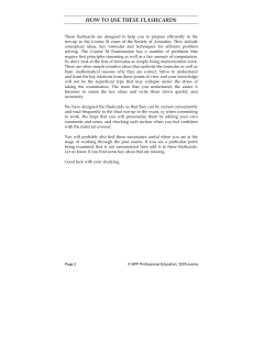


© Copyright 2026