
ANALYSIS OF NATURALLY OCCURRING RADIONUCLIDES IN FLY ASH AND GYPSUM SAMPLES By
ANALYSIS OF NATURALLY OCCURRING
RADIONUCLIDES IN FLY ASH AND GYPSUM SAMPLES
By
Angela R. Roper
Thesis
Submitted to the Faculty of the
Graduate School of Vanderbilt University
in partial fulfillment of the requirements
for the degree of
MASTER OF SCIENCE
In
Physics
August, 2012
Nashville, Tennessee
Approved
Professor Michael G. Stabin
Professor David S. Kosson
i
ACKNOWLEDGEMENTS
I would like to thank her thesis advisor, Dr. Michael Stabin, this work would not have
been possible without his guidance, encouragement and unlimited patience. He has started me
down the path to being a great academic researcher, and I am indebted to him. He will always
be my teacher and mentor. I would like to thank Dr. David Kosson for not only giving me the
opportunity to research this subject matter but to collaborate with him as well.
This work would not have been possible without finical support of grant 38-10-948 from
the Nuclear Regulatory Commission. I would like to acknowledge the US EPA Office of Research
and Development (S. Thorneloe, Research Triangle Park, NC) and ARCADIS U.S., Inc. (P. Kariher,
Research Triangle Park, NC) for providing CCR samples used in this project.
I would like to thank the individuals that contributed to this work including Rossane
Delapp, Susan Kost, and Dr. Hamp Turner. I am appreciative of the Department of Physics and
Astronomy for having me as a student, and the Department of Civil and Environmental
Engineering for adopting me as one of their own.
I would like to thank my family for their support, their love and guidance was invaluable
to the completion of this work. I would like to thank my parents for their direction and
unconditional love.
ii
TABLE OF CONTENTS
ACKNOWLEDGEMENTS ................................................................................................................... II
LIST OF TABLES ................................................................................................................................ V
LIST OF FIGURES ............................................................................................................................ VII
I. INTRODUCTION ........................................................................................................................ 1
II. LITERATURE REVIEW ............................................................................................................... 7
Pathways to radiation dose ..................................................................................................... 7
Literature on specific activity of fly ash and other pertaining material ................................ 13
Literature on 222Rn internal dose........................................................................................... 23
Gamma spectroscopy ............................................................................................................ 24
Literature on Monte Carlo simulations and external dose ................................................... 31
III. METHODS AND MATERIALS ................................................................................................. 33
Sample specific activity methods and materials ................................................................... 33
Headspace methods and materials ....................................................................................... 40
222
Rn dose methods and materials ........................................................................................ 43
Monte Carlo external dose methods..................................................................................... 44
Specific activity of fly ash, gypsum and other ....................................................................... 47
Headspace comparison ......................................................................................................... 58
Internal dose due to 222Rn ..................................................................................................... 62
External dose from Monte Carlo simulations........................................................................ 64
Cumulative dose for male, female and child (male 10 years old) ......................................... 75
Comparison results ................................................................................................................ 84
IV. DISCUSSION ......................................................................................................................... 88
Specific activity analysis......................................................................................................... 88
Headspace analysis ................................................................................................................ 89
Radon internal dose analysis ................................................................................................. 90
Monte Carlo external dose analysis ...................................................................................... 91
Internal and external total dose analysis .............................................................................. 93
iii
`
V. CONCLUSIONS....................................................................................................................... 95
APPENDIX A ............................................................................................................................... 97
REFERENCES ............................................................................................................................ 102
iv
LIST OF TABLES
Table 1. Specific activity throughout the combustion process. ................................................... 16
Table 2. Fly ash concentrations reported by other investigators (Bq kg-1). ................................. 17
Table 3. Coal concentrations reported by other investigators (Bq kg-1). ..................................... 18
Table 4. Cement concentrations reported by other investigators (Bq kg-1)................................. 19
Table 5. Concrete concentrations reported by other investigators (Bq kg-1). .............................. 20
Table 6. Soil concentrations reported by other investigators (Bq kg-1)........................................ 20
Table 7. Natural gypsum concentrations reported by other investigators (Bq kg -1).................... 21
Table 8. Brick concentrations reported by other investigators (Bq kg-1). .................................... 21
Table 9. Stone and rock concentrations reported by other investigators (Bq kg -1). .................... 22
Table 10. 222Rn inhalation (µSv y-1) with varying emanation coefficients. ................................... 24
Table 11. Bituminous fly ash concentrations (Bq kg-1). ................................................................ 48
Table 12. Sub-bituminous fly ash concentrations (Bq kg-1). ......................................................... 49
Table 13. Gypsum concentrations (Bq kg-1). ................................................................................. 50
Table 14. Scrubber sludges and fixated scrubber sludges concentrations (Bq kg -1). ................... 51
Table 15. 238U concentrations in the larger containers (headspace) and Petri dishes (no
headspace)............................................................................................................................. 58
Table 16. 232Th concentrations in the larger containers (headspace) and Petri dishes (no
headspace)............................................................................................................................. 59
Table 17. 40K concentrations in the larger containers (headspace) and Petri dishes (no
headspace)............................................................................................................................. 60
Table 18. Doses from 222Rn inhalation (mSv y-1), occupancy of 100%, concrete concentration 40
Bq kg-1. ................................................................................................................................... 62
Table 19. Doses from Indoor 222Rn inhalation (mSv y-1) occupancy of 65% and 25%; concrete
concentration assuming 40 Bq kg-1. ...................................................................................... 63
Table 20. External dose (mSv y-1), occupancy of 100%, adult male. ............................................ 64
Table 21. External dose (mSv y-1), occupancy of 65%, adult male. .............................................. 65
Table 22. External dose (mSv y-1), occupancy of 25%, adult male. .............................................. 66
Table 23. External dose (mSv y-1), occupancy of 100%, adult female. ......................................... 67
Table 24. External dose (mSv y-1), occupancy of 65%, adult female. ........................................... 68
Table 25. External dose (mSv y-1), occupancy of 25%, adult female. ........................................... 69
Table 26. External dose (mSv y-1), occupancy of 100%, 10 year old male.................................... 70
Table 27. External dose (mSv y-1), occupancy of 65%, 10 year old male...................................... 71
Table 28. External dose (mSv y-1), occupancy of 25%, 10 year old male...................................... 72
Table 29. External dose halfway across room ( mSv y-1), occupancy of 100%, adult male,
10x12x8 ft3. ............................................................................................................................ 72
v
Table 30. External dose halfway across room ( mSv y-1), occupancy of 65%, adult male, 10x12x8
ft3. .......................................................................................................................................... 73
Table 31. External dose halfway across room ( mSv y-1), occupancy of 25%, adult male, 10x12x8
ft3. .......................................................................................................................................... 73
Table 32. External dose three quarters across room ( mSv y-1), occupancy of 100%, adult male,
10x12x8 ft3. ............................................................................................................................ 73
Table 33. External dose three quarters across room ( mSv y-1), occupancy of 65%, adult male,
10x12x8 ft3. ............................................................................................................................ 74
Table 34. External dose three quarters across room ( mSv y-1), occupancy of 25%, adult male,
10x12x8 ft3. ............................................................................................................................ 74
Table 35. Total dose (mSv y-1), occupancy of 100%, adult male. ................................................. 75
Table 36. Total dose (mSv y-1), occupancy of 65%, adult male. ................................................... 76
Table 37. Total dose (mSv y-1), occupancy of 25%, adult male. ................................................... 77
Table 38. Total dose (mSv y-1), occupancy of 100%, adult female. .............................................. 78
Table 39. Total dose (mSv y-1), occupancy of 65%, adult female. ................................................ 79
Table 40. Total dose (mSv y-1), occupancy of 25%, adult female. ................................................ 80
Table 41. Total dose (mSv y-1), occupancy of 100%, 10 year old male. ........................................ 81
Table 42. Total dose (mSv y-1), occupancy of 65%, 10 year old male. .......................................... 82
Table 43. Total dose (mSv y-1), occupancy of 25%, 10 year old male. .......................................... 83
Table 44. Total dose (mSv y-1), occupancy of 100%. ..................................................................... 84
Table 45. Total dose (mSv y-1), occupancy of 65%. ....................................................................... 85
Table 46. Total dose (mSv y-1), occupancy of 25%. ....................................................................... 86
Table 47. External dose with center room offset (mSv y-1), occupancy of 100%, adult male,
10x12x8 ft3. ............................................................................................................................ 86
Table 48. External dose with center room offset (mSv y-1), occupancy of 65%, adult male,
10x12x8 ft3. ............................................................................................................................ 87
Table 49. External dose with center room offset (mSv y-1), occupancy of 25%, adult male,
10x12x8 ft3. ............................................................................................................................ 87
vi
LIST OF FIGURES
Figure 1. Energy production and usage in the United States. ........................................................ 1
Figure 2. 2010 Coal Combustion Product survey............................................................................ 2
Figure 3. 238Uranium decay series................................................................................................... 4
Figure 4. 232Th decay series. ............................................................................................................ 5
Figure 5. 40K decay scheme. ............................................................................................................ 6
Figure 6. Conceptual site model with groundwater contamination pathway. ............................ 10
Figure 7. US Geological Survey for natural radiation. .................................................................. 13
Figure 8. Mean diameter of ash throughout the combustion process. ....................................... 16
Figure 9. Electron-hole pair production........................................................................................ 25
Figure 10. Canberra HPGe detector. ............................................................................................. 26
Figure 11. Typical gamma spectrum. ............................................................................................ 28
Figure 12. Compton scattering. .................................................................................................... 29
Figure 13. Efficiency plot of an HPGe detector. ............................................................................ 30
Figure 14. Ortec gamma spectrum. .............................................................................................. 34
Figure 15. Ortec energy calibration. ............................................................................................. 35
Figure 16. Ortec efficiency calibration curve. ............................................................................... 37
Figure 17. Secular equilibrium plot. .............................................................................................. 38
Figure 18. Petri dish, and polypropylene jars for samples and standard and for calibration ...... 41
Figure 19. Sample containers showing airspace above sample material. .................................... 41
Figure 20. Sample containers showing the diameter of the containers. ..................................... 42
Figure 21. Monte Carlo simulation geometry............................................................................... 46
Figure 22. 238U results from this study, compared to values observed in the literature. ............ 52
Figure 23. 232Th results from this study, compared to values observed in the literature. ........... 53
Figure 24. 40K results from this study, compared to values observed in the literature. .............. 54
Figure 25. 238U concentrations; error bars are ± 1 standard deviation. ....................................... 55
Figure 26. 232Th concentrations; error bars are ± 1 standard deviation....................................... 56
Figure 27. 40K concentrations; error bars are ± 1 standard deviation. ......................................... 57
Figure 28. Variability of the natural radiation background in the US. .......................................... 94
Figure 29. Certificate of calibration for standard source. ............................................................ 97
Figure 30. QA sheet for Ortec detector. ....................................................................................... 98
Figure 31. Detector specs for Canberra detector. ........................................................................ 99
Figure 32. Standard Cs-137 QA graph for Canberra detector. ................................................... 100
Figure 33. 352 keV background QA graph for Canberra detector. ............................................. 101
vii
CHAPTER I
INTRODUCTION
Exposure to humans to natural radiation from cosmic rays and from soil is an everyday
occurrence. In addition to those forms of radiation, radionuclides from building materials may
cause further exposures. The burning of coal is a significant element in the US energy budget;
Figure 1* shows the primary forms of energy production in the United States.
Figure 1. Energy production and usage in the United States.
*
http://www.eia.gov/energy_in_brief/major_energy_sources_and_users.cfm
1
Coal fired power plants (CPPs) release naturally occurring radioactive material during
the combustion of coal. Fly ash, a by-product of CPPs, has many beneficial applications, for
example in roads, building materials, concrete, cement and other materials. From a survey
from American Coal Ash Association (ACAA 2010) 6.77x10⁷ short tons of fly ash were produced
in 2010 and 2.57x10⁷, 37.9%, was used beneficially, this percentage substantially greater than
many countries (Baykal et al. 2011, Papastefanou 2010). Figure 2 shows results of a survey
regarding fly ash use, along with other CCRs that can be used beneficially.
Figure 2. 2010 Coal Combustion Product survey.
2
However, use of fly ash has come under scrutiny due to recent accidents, as well as a
general interest in evaluating the possible dosimetric consequences for humans of use of this
material in these applications. A notable fly ash spill occurred in Kingston, TN at a facility
owned by the Tennessee Valley Authority (TVA) in 2008, in which over a billion gallons of fly ash
and coal slurry were spilled due to a disposal cell rupture. This was the largest spill of this
nature to occur in United States history. The Environmental Protection Agency (EPA) has thus
decided to review their policies on regulation of fly ash. The EPA’s proposal has two options, to
regulate coal combustion residues (CCRs) under subtitle C as special wastes or under subtitle D
as non-hazardous waste (40 CFR 75(118) 35128-35264); both options would operate under The
Resource Conservation and Recovery Act (RCRA). Beneficial use of fly ash could be affected by
this decision, though usage eliminates waste and saves money. Fly ash as an additive in
concrete not only reduces the amount of waste products produced by CPPs but also increases
the robustness of concrete by increasing the strength and durability of the concrete (Baykal and
Saygili 2011).
In this work, analyses of the radioactive content of samples of fly ash were performed
to determine if beneficial uses of fly ash in building materials could be of radiological concern.
Analysis was also performed on samples of gypsum, scrubber sludge and fixated scrubber
sludge. The content of 234U and 232Th decay series radionuclides, as well as of 40K, was
determined via gamma spectroscopy. Figures 2and 3 show the uranium chain and thorium
decay series.
3
Figure 3. 238Uranium decay series†.
†
ICRP 2012
4
Figure 4. 232Th decay series‡.
‡
ICRP 2012
5
40
K is not part of a decay series; it’s 1461 keV gamma is the key gamma.
Figure 5. 40K decay scheme.
After determination of typical fly ash radionuclide concentrations, a dosimetric analysis was
performed using Monte Carlo transport simulations in concrete structures of various sizes
assumed to contain different levels of incorporated fly ash.
6
CHAPTER II
LITERATURE REVIEW
Pathways to radiation dose
Radiation is ubiquitous; ionizing radiation from space constantly bombards our
atmosphere and naturally occurring radionuclides are present in soil, water, food, air, and the
human body. Radionuclides were produced when the universe first formed, although many
have decayed away since their creation. Three important naturally occurring radionuclide
decay chains – the uranium series, thorium series and actinium series, plus the radionuclide 40K
provide significant contributions to our external background radiation. 226Ra, a daughter
product of uranium, is responsible for the major fraction of internal dose, whether from
ingestion or inhalation through 222Rn gas. Uranium is present in soil and groundwater, which
contribute to human exposures through internal and external exposure pathways.
When radiation was first discovered there was little understanding of the potentially
deleterious effects of ionizing radiation to humans. Medical uses of x-rays and 226Ra
proliferated in the early 1900s, as the benefits of the medical uses of radiation began to be
realized. But soon, short and long term effects of radiation were beginning to be understood. In
1925, Dr. A. Mutscheller suggested a limiting dose of 1/100 of a threshold erythema dose per
month, an “R-unit.” Simple limits of dose to the whole body to 1/10 of a 'skin erythema dose'
per year, and an internal limit of 0.1 µg of radium in the body were proposed in 1941. Over
subsequent decades, the international scientific community studied these effects extensively,
7
and dose limits were refined; finally in 1959 the ICRP released a report in the Health Physics
Journal that laid the basis for a comprehensive system of radiation protection for radiation
workers and the public. This work was mostly adopted and released as the first formal national
US regulation of radiation exposures, Title 10 of the Code of Federal Regulations, Part 20, i.e.
10CFR20. (Stabin 2007).
Today, there are many laws regarding contamination from radiation exposure and
inhalation, chemical toxicity, air pollution and water pollution. Throughout the 1950s and
1960s, a general realization grew in the US of the need to formalize a regulatory basis for
protection of the environment from all forms of potential chemical and radiological damage,
and this led to the formation of the Environmental Protection Agency (EPA) in 1970. In the
recent years, nuclear regulations and policies have received heightened scrutiny because of the
disaster at the Fukushima nuclear installation and debate over the high level waste (HLW)
geologic repository in Yucca Mountain, Nevada. Some of the major laws regulating nuclear
materials and waste are listed below (Clarke 2012)
8
One of the most important regulations is the Atomic Energy Act (AEA) of 1954. It is the law that
governs nuclear materials and waste, and both the Nuclear Regulatory Commission (NRC) and
the EPA draw their enforcement jurisdiction from this act. The Nuclear Waste Policy Act (NWPA)
of 1983 was established to develop a geologic repository for high level wastes (HLW) from the
operation of nuclear power plants. The act authorized the creating of a repository, which after
much study and expenditure of federal funds was determined to be in Yucca Mountain,
Nevada. Due to political reasons, use of this site, as of this writing, has been put on hold
indefinitely.
The EPA also established laws relating to environmental contamination such as the Safe
Drinking Water Act (SDWA) and the Clean Air Act (CAA), which set limits of permissible levels of
contaminates, both radioactive and chemical. The EPA also oversees implementation of the
RCRA, which covers solid and hazardous waste. RCRA is important to this study because this is
the act that will govern fly ash disposal, either under Subtitle C as hazardous waste or under
Subtitle D as “special waste.” However, currently, and perhaps in the future, fly ash is
exempted from RCRA under the Bevell Amendment. When regulating hazardous materials, the
EPA considers all avenues of contamination and the best analysis of possible receptors is to
build a site conceptual model as in Figure 6 (Brown 2008).
9
Figure 6. Conceptual site model with groundwater contamination pathway.
When overseeing the release of contaminates, such as the fly ash spill in Tennessee in 2008, the
EPA uses such conceptual site models to determine the type of effect releases of this kind could
have on the air, water, biota and many other factors.
Since the EPA, NRC and other regulatory bodies have been overseeing releases of
radioactive materials to the environment, there have been areas found that have elevated
concentrations of some radionuclides. For those that live in those areas, depending on the
method of contamination, there are ways to circumvent this problem. For example, water
supplies in the Atlantic coastal plain areas and piedmont provinces were found to exceed the
existing radium limit of 185 Bqm-3 (5 pCiL-1) (Lucas 1982, EPA 1991) with a maximum of 958
10
Bqm-3 (Hess 1985 et al.). A study was performed to determine the most effective water
treatment method. Reverse osmosis and sodium ion-exchange processes were 92% effective
and lime-soda ash softening processes reduced concentrations from 75 to 95% (Brinck et al.
1978).
Areas with high indoor radon have been discovered, e.g. the now famous Watras house
in Pennsylvania. Mr. Watras worked at a nuclear power plant and set off radiation monitors
consistently. It was determined that the radiation was of natural origin, and the Watras home
was tested for 222Rn; the indoor radon concentration was found to be 100 kBq m-3 (2700 pCi L1
). The Watras were advised to vacate the premises by the Pennsylvania Department of Energy
Resources. This event has widely been seen as the triggering point that led to the Indoor
Abatement Act, which led to research of indoor radon concentrations (Cole 1993).
Fortunately, there are ways to reduce exposures to radon gas. A simple way is to use air
filtration systems or fans throughout the home to increase air turnover (Curling et al. 1990a,b).
One may seal openings in the foundations of the home or use “sub-slab suction” devices to
draw out the gas (Eisenbud and Gesell 1997). It is important to note that while exposure to
high levels of radon may be potentially dangerous, most levels are low and if higher
concentrations can be managed with the abatement methods described above. Risk informed
regulations should be implemented, so as to balance cost and benefit (Clarke 2012).
All building materials contain radionuclides at some levels Using fly ash in concrete,
increases the durability of the concrete, reduces the need to utilize natural resources and it
eliminates costly waste, but may raise the dose from naturally occurring radionuclides present
in the coal combustion residues.
11
Inhalation of radon gas is one of two pathways humans can receive a radiation dose
from fly ash within building materials, the second being external dose by gamma rays. Fly ash
contains radionuclides from the uranium series, thorium series and 40K. These nuclides emit
alpha, beta and gamma radiation. While alpha and beta radiation are particles will be absorbed
within the walls, gamma radiation is an electromagnetic wave and can penetrate through the
walls. However, both the uranium and thorium series have radon isotopes; radon is a noble gas,
and so can diffuse out of the concrete. It and its progeny emit alpha, beta and gamma radiation.
The dose one receives depends on the porosity of the concrete, the air exchange rate in the
room, the occupancy, distance and percentage of the concrete/fly ash mixture. The radon itself
is inhaled and exhaled quickly, but the progeny are usually attached to dust particles, due to
their electrostatic charge, and may be deposited on the walls of the respiratory tract and
deliver dose to important tissues there over their longer retention time (Eisenbud 1997).
12
A study from the US Geological Survey (USGS 1997) concluded that the majority of our
radiation exposure comes from natural sources.
Figure 7. US Geological Survey for natural radiation.
Most of the radiation dose we receive actually comes from natural sources – natural radon,
cosmic radiation and terrestrial from the soil. Furthermore, all building materials are
radioactive to some extent, whether from natural or artificial origin.
Literature on specific activity of fly ash and other pertaining material
There are conflicting views as to whether use of fly ash could represent a significant risk
to human health. A study from the European Commission (EC 112) found that there was
potential to have annual exposures above 1 mSv in buildings with concrete containing a high
13
percentage of fly ash and possible if the use natural building stones are used in bulk amounts.
They defined an 'activity concentration index' (I) for identifying whether a dose criterion is met
using the following formula:
Where CRa, CTh, CK is the specific activity of 226R, 232Th, 40K. The activity concentration index
should not exceed the following values below depending on the dose criterion and the way and
the amount the material is used in a building.
The study also found one could get an annual effective dose of about 0.25 mSv in addition to
the dose received outdoors living in an apartment block made of concrete with average
concentrations of 40, 30, and 400 Bq kg-1 for radium, thorium and potassium respectively
(Markkanen 1995).
The most common method to determine the specific activity of these materials is
gamma ray spectroscopy using HPGe (El Afifi et al. 2006), but other methods may be used, such
as alpha particle spectrometry, beta particle counting or gamma measurements after
radiochemical separation (Johnston 1997, Koler 2002). Also, it has been pointed out that radon
14
isotopes may not necessarily be in secular equilibrium with parent nuclides due to geo-chemical
processes (Kovler et al. 2005).
Specific activities for fly ash, building materials and other sources have been given in
Tables 2-9. Turhan et al. (2010) evaluated fly ash concentrations of 238U§, 232Th, and 40K and
found values between 17 to 2720, 9 to 696, 12 to 2974 Bq kg-1, respectively. This is a
considerable range, and many of the literature values have wide a wide range. Coles et al.
(1978), in a domestic study, the range was decreased and found lower overall maximum
concentrations, with 238U, 232Th, and 40K values between 70 to 130, 63 to 89, 233 to 300 Bq kg-1,
respectively. Similar results were given in a European Commission study (EC 112 1999), which
showed a much higher range of concentrations, with means of 180, 100, 650 Bq kg-1 for 238U,
232
Th, and 40K. Other studies have found concentrations of 117.5, 126.8, 687 and 134.2, 74.7,
646.9 Bq kg-1 for 238U, 232Th, and 40K (Nakaoka et al. 1984, Bem et al. 2002). Literature values
for natural gypsum have average means of 15, 13.6, 112 for 238U, 232Th, and 40K (EC 112 1999,
Trevisi et al. 2012, El Afifi et al. 2006, NCRP 1987).
The specific activity in uranium and radium is related inversely to the diameter of the
ash. Also, fly ash size varies depending on the stage within the coal fired power plant;
Papastefanou (2010) took fly ash from three separate stages in the combustion process and
found as the ash flows towards the stack, they decrease in diameter, as seen from below.
§
Assuming secular equilibrium with
226
Ra and
238
U
15
Figure 8. Mean diameter of ash throughout the combustion process.
Table 1. Specific activity throughout the combustion process.
The specific activities are seen to be different by as much as a factor of two depending on the
point in combustion.
16
Table 2. Fly ash concentrations reported by other investigators (Bq kg-1).
238
Mean
232
Max
356
263
950
574
460
870
97
44
169
Mean
100
40
Th
Min
Max
300
Mean
650
K
Min
Source
Max
1500
297
204
382
102
9
696
517
12
2974
74
33
126
728
185
1547
132
107
207
268
56
348
118
106
124
127
114
13
687
618
722
89
76
114
91
57
130
364
170
615
111
90
126
75
48
92
647
449
758
63
89
233
300
134
Mean
Standard
deviation
Min
Max
U
Min
94
185
70
130
228
159
363
101
65
198
520
241
1016
197
89
574
151
44
460
375
114
950
22
74
132
37
9
114
203
13
696
186
268
728
200
12
618
868
300
2974
EC 112 (1999)
Papastefanou
(2010 )
Papastefanou et
al. (1979)
Turhan et al.
(2010)
Tomczynska et
al. (1980 )
Mirshra et al.
(1984)
Nakaoka et al.
(1984)
Fardy et al.
(1989)
Hayumbu et al.
(1995)
Bem et al.
(2002)
Coles et al.
(1978)
Coal, like fly ash, can be highly variable in radionuclide concentration. One study found
the specific activity of uranium to be as high as 15,000 Bq kg-1 in coal from Freital, Germany
(Vandenhove 2000). Others have found 1,480 Bq kg-1 of 226Ra in coal samples from Illinois and
2,590 Bq kg-1 of 226Ra in coal from Northern Greece (Barber and Giorgio 1977, Papastefanou
and Charalambous, 1979, 1980).
17
Secular equilibrium between 238U and 226Ra in fly ash has been contested by many
(Kovler et al. 2005, Papastefanou and Charalambous, 1979, 1980) but it is usually assumed for
coal (Coles et al. 1978). One study hypothesized an surplus of 238U due to precipitation in
reduction zones in coal mines or removal of 234U by flowing waters (Papastefanou 2010).
Table 3. Coal concentrations reported by other investigators (Bq kg-1).
238
232
U
Mean
18
Mean
Stdev
Min
Max
40
Th
Min
1
Max
540
9
32
385
298
435
38
2
141
12
24
6
13
16
39
243
12
416
117
399
144
177
12
416
64
111
1
298
Mean
21
K
Min
2
Max
320
6
21
30
37
9
26
107
48
13
14
7
9
19
153
8
229
222
16
540
20
11
8
37
10
8
2
26
111
115
19
320
Mean
52
Source
Min
1
Max
710
27
52
294
95
37
7
759
200
72
40
180
108
26
106
59
227
108
87
26
294
29
22
1
59
355
301
52
759
Beck, DOE - 1980
Coles et al.(1978 US)
Papastefanou et al.
(1979)
Tomczynska et al.
(1980)
Mishra et al. (1984)
Nakaoka et al.
(1984)
Bem et al. (2002)
Papastefanou
(2010)
Tracy et al. (1985)
Font et al. (1993)
World average building material specific activity has been cited to be 50, 50, and 500 Bq
kg-1, with world average soil levels of 35 (17-60), 30 (11-64), 400 (140-850) Bq kg-1 for 226Ra,
232
Th, and 40K respectively (UNSCEAR 1993, UNSCEAR 2000). Radiation exposures from
18
radionuclides in building materials depend on the type of materials used; wood for example,
does not have much radioactivity but it shields less from cosmic radiation. Soil concentrations
can be highly variable, with levels reported as high as 1,000 Bq kg-1 for 238U, 360 Bq kg-1 for
232
Th and 3,200 Bq kg-1 for 40K (UNSCEAR 2008).
Table 4. Cement concentrations reported by other investigators (Bq kg-1).
238
232
U
Mean
18
Max
Mean
Min
K
Max
Mean
14
48
293
115
46
59
29
24
27
23
19
132
37
21
564
273
432
422
832
230
506
173
237
38
18
18
51
39
34
14
132
371
208
115
832
51
Mean
Stdev
Min
Max
Min
40
Th
19
Min
Source
Max
Ramadan et al.
(2006)
Beretka et al. (1985)
Malancea et al.
(1993)
Khan et al. (2001)
Kumar et al. (1999)
Amrani et al. (2001)
Ibrahim (1999)
Ackers et al. (1985)
Mollah et al. (1986)
Xinwei (2005)
NCRP (1987)
Table 5. Concrete concentrations reported by other investigators (Bq kg-1).
238
Mean
Limestone
Sandstone
31
1
Mean
Stdev
Min
Max
16
21
1
31
232
U
Th
Min Max Mean Min
30
40
37
12
35
1
9
9
19
89
15
K
Max Mean Min
190
400
190
430
65
354
95
152
392
7
89
385
120
260
30
16
19
41
133
54
65
190
435
489
89
780
27
14
9
40
16
15
1
37
40
342
126
89
430
163
135
7
290
Source
Max
1600
1600
766
1450
EC 112 (1999)
EC 112 (1999)
Ademola (2005)
Trevisi (2012)
NCRP (1987)
NCRP (1987)
1100 (Eicholz, 1980)
1269
335
766
1600
Table 6. Soil concentrations reported by other investigators (Bq kg-1).
238
US
World
Mean
Stdev
Min
Max
Mean
35
33
22
30
7
22
35
U
Min
4
4
---4
4
232
Max
140
140
---140
140
Mean
35
45
37
34
38
5
34
45
40
Th
Min
4
Max
130
1
258
Mean
370
420
400
483
3
2
1
4
194
91
130
258
418
48
370
483
20
K
Min
100
Source
Max
700
0
3200
50
71
0
100
1950
1768
700
3200
UNSCEAR(2000)
UNSCEAR (2000)
NCRP(1987)
UNSCEAR (2010)
Table 7. Natural gypsum concentrations reported by other investigators (Bq kg -1).
238
Mean
232
U
Min
Max
15
Mean
Stdev
Min
Max
15
---15
15
-------------
40
Th
Mean Min
10
--------------
9
28
7
1
25
14
10
7
28
13
17
1
25
K
Max Mean Min
80
100
100
91
5
30
129 126
148
77
40
30
100
112
32
80
148
66
86
5
126
Source
Max
EC 112 (1999)
Mustonen (1997)
Trevisi et al. (2012)
El Afifi et al. (2006)
NCRP (1987)
200
279
132
204
74
132
279
Table 8. Brick concentrations reported by other investigators (Bq kg-1).
238
232
U
Mean
Min
Max
Clay (red)
Sand-lime
4
Range
Clay
Mean
Stdev
Min
Max
Mean
50
10
180
48
11
111
111
---111
111
40
Th
4
180
4
0
4
4
180
0
180
180
30
22
10
50
Min
K
1
2
Max
200
310
140
164
1
140
1
1
1
2
191
71
140
310
21
Mean
670
640
598
636
36
598
670
Min
Source
7
12
Max
2000
4000
1200
1169
7
1200
9
3
7
12
1914
1218
1169
4000
EC 112 (1999)
EC 112 (1999)
Eicholz (1980)
Trevisi (2012)
NCRP (1987)
Eicholz (1980)
Table 9. Stone and rock concentrations reported by other investigators (Bq kg-1).
238
232
U
Mean
Min
40
Th
Max
Mean
Min
K
Max
60
Mean
Min
4000
Igneous
48
48
810
Sandstone
15
24
330
Shales
15
41
810
Limestone
Igneous - Basalt
Igneous - Mafic
Igneous - Salic
Igneous Granite
Shale
sandstones
Clean quartz
Igneous
plutonic
Igneous
volcanic
15
5
81
300
10
Max
640
310
7
Source
10
15
10
60
10
80
70
1100
40
70
1000
40
50
400
1500
NCRP (1987)
800
10
8
300
89
0
906
1049
24
2040
163
8
750
1295
170
2354
Metamorphic
21
0
142
395
0
1891
Granite
70
65
75
1560
1340
1780
56
42
5
163
17
27
0
65
315
367
8
906
734
449
81
1560
529
589
0
1340
1783
1166
300
4000
Mean
Stdev
Min
Max
30
19
10
60
7
---7
7
10
0
10
10
EC 112 (1999
- Europe)
Mustonen et.
al (1997)
UNSCEAR
(1958)
UNSCEAR
(1958)
UNSCEAR
(1958)
UNSCEAR
(1958)
NCRP (1987)
NCRP (1987)
NCRP (1987)
NCRP (1987)
NCRP (1987)
Trevisi et. al
(2012)
Trevisi et. al
(2012)
Trevisi et. al
(2012)
El Afifi et. al
(2006)
When fly ash is used as an additive in concrete, the increase of radionuclide
concentration is only about 3 percent in comparison to other building materials, such as red
22
brick, that contain higher natural concentrations of radionuclides (Eisenbud 1997). Direct
measurement of the increase in radon is difficult because radiation emanation from the soil
below the dwelling, which dominates the radon inhalation over building materials and other
sources (Eisenbud and Gesell 1997). However is it is estimated that concrete of all types only
contribute less than 10 percent of the indoor radon dose (Eisenbud 1997). Of more concern
from CCRs might include the leaching of constituents like arsenic, selenium and lead into
groundwater but concentrations of these elements are variable from site to site (Eisenbud
1997).
Literature on 222Rn internal dose
Addition of fly ash to concrete may have an effect on the radon exhalation rate, but
surprisingly there are several literature sources that claim that it has no effect (Ulbak et al.
1984, Van Dijk et al. 1991) and maybe even causes a reduction in the radon 'exhalation rate'
(Stranden, 1983, Ackers et al. 1985, Kovler et al. 2005). Others disagree and believe that the
addition of fly ash to concrete increases the radon exhalation rate (Siotis et al. 1984). Kolver et.
al 2005 calculated a typical dose due to 222Rn to 0.227 mSv y-1, assuming an 'emanation
coefficient', the fraction of radon that escape from a material, of 5%. Dose from 220Rn was only 9.5
µSv y-1 for the same emanation coefficient, so doses from 220Rn are low and are of very little
importance compared to that from 222Rn. A study was done for emanation factors of 1,5,10
and 15 percent; dose from radon increased with increases in the emanation factor (Kolver et al.
2005). The final results showed a reduction in radon emanation due to the 0.52 percent
emanation coefficient of fly ash, compared to the 7.65 percent coefficient of Portland cement,
23
despite the fly ash being three times higher in 226Ra content. The dose depends on the area in
question as well, whereas this study was done with small rooms vs. larger volumes (TaylorLange et al. 2012). It is debatable which is the best emanation coefficient to be used, one
study found the best number to use would be 5%, while another believed it should be given in a
range of 2-5%, and another used a variety of different ones but believed the best to 5% as well
(Siotis et al, 1984 Stranden 1983, Taylor-Lange et al. 2012).
Table 10. 222Rn inhalation (µSv y-1) with varying emanation coefficients.
Description
No fly ash
25% fly ash,5% emanation
1% emanation
5% emanation
10% emanation
µSv y-1 due to 222Rn inhalation
< 54
95
44
227
455
Source
Taylor-Lange et. al 2012
Taylor-Lange et. al 2012
Kolver et. al 2005
Kolver et. al 2005
Kolver et. al 2005
Gamma spectroscopy
For this experiment two p-type coaxial high purity germanium detectors (HPGe) were
used for gamma counting. The detectors have a P-I-N structure, which means there in an
Intrinsic (I) region is sensitive to the ionizing radiation from the X-rays and gamma rays. When
under a reverse bias, an electric field extends across the depleted region, also known as the
intrinsic region. When photons interact within the depleted region charge carriers, namely
holes and electrons, are produced and are swept away by the electric field to the P and N
electrodes. This charge is proportional to the energy deposited by the photon and it is
24
converted into a voltage pulse by an integral charge-sensitive preamplifier. The process is
illustrated in Figure 9**.
Figure 9. Electron-hole pair production.
These detectors have a low band gap and must be cooled by liquid nitrogen to reduce the
reverse leakage current to an acceptable level; otherwise noise destroys the energy resolution.
Coaxial HPGe detectors have a high efficiency, high resolution and it takes little energy (~1.1 eV)
to produce charge carriers, which makes it perfect for the current study (Canberra 1998).
Figure 10 shows a diagram of a typical Canberra HPGe detector††.
** http://www4.nau.edu/microanalysis/Microprobe/EDS-Detector.html
††
http://www.df.uba.ar/users/sgil/labo5_uba/recursos/Gamma_Detection_Canberra.htm
25
Figure 10. Canberra HPGe detector.
In any radiation counting, one must understand the counting system's detection limits;
with samples containing environmental levels of radioactivity, concentrations often may be
close to detection limits. The key quantity determining detectability is the Lower Limit of
Detection (LLD) (Currie 1968). Expressed mathematically this is:
where
=√
, with NB being the number of background counts
LLD is defined as the counts above background that can be seen with a 5% chance of
making a Type I or Type II error. A type I error is an error in which a background count is called
a positive count, and a Type II error is an error in which a positive count is called a background
count. The Minimum Detectible Activity (MDA) is the lowest level of activity that can be seen
at the LLD. The equation for MDA is (Currie 1968, Knoll 2000):
26
where f = radiation yield per disintegration
= absolute detection efficiency
T = counting time
Currie (1968) goes on to define three regions in which the analyst’s confidence can be defined.
1. LC (critical level) – the activity is different from zero with 95% confidence. LC = 2.33
2. LD (detection level) – also known as the MDA, smallest true signal that can be detected,
it keeps the Type I and II errors to 5%.
3. LQ (determination level) – the true value of the net signal has a relative standard
deviation of 10%. Mathematically it is
{
[
]
}
Currie really recommended that quantitative assessment be done only above LQ, however, the
majority of health physicists are comfortable reporting values above LD (the MDA), and for this
study MDAs were used to define the limit at which numerical values were reported (Currie
1968, Stabin 2000). One can extend this to be a minimum detectible activity concentration (Bq
kg-1) by dividing by the sample mass.
In gamma spectrometry, one must look at the spectrum of detected photons and
determine the origin of the peaks. An example spectrum can be seen below‡‡.
‡‡
http://www.pas.rochester.edu/~AdvLab/6-Gamma/Lab06%20GammaSp.pdf
27
Figure 11. Typical gamma spectrum.
The spectrum shows the gamma photopeaks of a typical radionuclide, as well as all the
interactions, including scattering events and other photopeaks. The three main photon
interactions of interest are photoelectric scattering, Compton scattering, and pair production.
When a photoelectric event occurs, the photon energy is completely absorbed, and the energy
event is shown as an event from a photon of this energy ('full energy' event in the diagram
above). Compton scattering occurs when a photon interacts with an orbital electron, the
photon is scattered in another direction and loses energy. The orbital electron is ejected from
the atom with the energy lost from the photon. The Compton equation is given as:§§
§§
http://hyperphysics.phy-astr.gsu.edu/hbase/quantum/compton.html
28
Figure 12. Compton scattering.
To get the equation in terms of energy we use
where
= Planck’s constant, 6.63*10-34 J-s
= frequency of the electromagnetic radiation s-1
λ = wavelength [m]
c = speed of light, 3*108 ms-1
where mo = the electron rest mass
Any and all scattering angles may occur in a given scattering event. Thus, a 'continuum' of
partial energy events will be shown in the spectrum (Figure 11, above) on which full photopeak
events are superimposed, representing partial photon deposition in the detector. However, if
one or more Compton events occur in the detector followed by a photoelectric event, all of this
29
energy will be scored within the detector event resolution time and will represent a full
photopeak event. If the photon energy is above 1.02 MeV, pair production events are possible.
In pair production, one or both of the 511 keV photons may be detected. If one is detected and
the other escapes, a ‘single escape peak’ results; if both annihilation photons escape the
detector, a ‘double escape peak’ is recorded. When two full photopeak events are detected at
the same time, it is registered as a photopeak event at the sum of the two photon energies,
thus representing a false 'sum peak'. After eliminating false peaks in a spectrum, true
photopeak events of parent or progeny nulcides are used to confirm identification of the key
photopeaks of interest. With nuclides in a decay chain in secular equilibrium, the areas under
the various photopeaks will be theoretically equal, when properly weighted for photon
abundance and detector efficiency at each energy.
A typical efficiency plot of HPGe detector is shown in Figure 13.
Figure 13. Efficiency plot of an HPGe detector.
30
The efficiency curve of a Ge detector consists initially of a quadratic function, then the tail turns
into a somewhat linear function, with the two being separated by a 'knee.'
Literature on Monte Carlo simulations
Monte Carlo simulation of radiation transport is a well-established and validated science.
Very simple codes can be written, for example to model photon attenuation in a uniform
medium. In most applications, however, the geometries and materials are complex, and
modeling of the transport of different types of radiation requires a complicated and well
validated code. Several of the widely available and used Monte Carlo codes are:
1. EGS4 (Ford and Nelson 1978) - electron gamma shower code, a general purpose code
for coupled transport of electrons and photons in different geometries for particles with
energies from a few keV to several TeV. Originally designed for modeling of radiation
therapy, but it can be used in external, internal and detector dose calculations.
2. MCNP (Briesmeister 1997) – Monte Carlo N-particle transport code, can be used for
neutron, photon, electron, or coupled neutron/photon/electron transport modeling in
complicated three-dimensional geometries. Originally designed for modeling of reactor
environments, but it can be used for external, internal, detector and many other dose
calculations.
3. ALGAMP (Ryman and Eckerman 1993) – Organ doses are calculated by scoring energy
deposition in all organs except skeletal tissues. It was the first to define all the original
absorbed fractions, and it was used for years in internal dosimetry. It was not
distributed widely, being mostly used within Oak Ridge National Laboratory in Oak
31
Ridge, TN, but it was used for many years to determine tables of absorbed fractions for
internal and external sources that were the basis for many important dosimetry
documents.
4. GEANT (Agostinelliae et al. 2003) - GEometry ANd Tracking, models a variety of different
particles over a range of 250 eV to TeV. Originally developed by CERN for high energy physics.
The latest generation of this software is Geant4,*** which is widely used in many applications
worldwide.
***
Copyright (c) Copyright Holders of the Geant4 Collaboration, 1994-2006.
32
CHAPTER III
METHODS AND MATERIALS
Sample specific activity methods and materials
Samples of bituminous fly ash (N = 30), sub-bituminous fly ash (N = 9), FGD gypsum (N =
20), and scrubber sludges and fixated scrubber sludges (N = 15) from US coals were analyzed
using two p-type High Purity Germanium (HPGe) photon detectors, one manufactured by
Canberra using the 'Genie 2000'††† software and the second by Ortec using the
'GammaVision'‡‡‡ software. The detectors were calibrated using a mixed nuclide NIST traceable
standard used from Eckert & Ziegler and was calibrated in 2008 with a total activity of 7.77x10⁴
Bq. The standard contains 100 grams of sand in a 250 mL polypropylene jar. The sample
containers were 250 mL (8 oz) polypropylene jars with a cap size of 89 mm from Fisher
Scientific. Samples were chosen to be around 40-50 g, so as to be similar to the counting
geometry of the standard. The atomic composition of the samples and density of the standard
were assumed to be reasonably similar.
Energy calibration of the detector with the standard was necessary before samples
could be counted. The procedure for energy calibration for the Ortec is as follows:
†††
‡‡‡
Copyright © 2001 Canberra Industries, Inc.
Copyright © 2003 Advanced Measurement Technology, Inc.
33
1. Place standard in the detector and count for five minutes.
2. Figure 14 shows a spectrum already calibrated with key gammas marked in red,
however, in this figure the calibration has already been done, with the 137Cs 661 keV
peak showing pertinent information. Before calibration this peak will not display the
radionuclide, since there is no information to understand the relationship between
channel number and absolute energy.
Figure 14. Ortec gamma spectrum.
3. From the spectrum peaks are highlighted and then the radionuclides are identified
using the standard calibration sheet, (Appendix A).
4. From the spectrum, the two well-known cobalt peaks at 1173 keV and 1332 keV are
easily identified. Other peaks are seen as well; this particular spectrum has
34
additional peaks at 60, 88, 122 and 662 keV for 241Am, 109Cd, 5757 and 137Cs
respectively. From these six radionuclides, an energy calibration can be completed.
5. Using the GammaVision software, one can input in these energies for each peak
highlighted as seen below, and a keV vs channel curve for the energy calibration is
created.
Figure 15. Ortec energy calibration.
The next step before counting samples is to do an efficiency calibration. The procedure
is as follows:
1. Obtain a spectrum from the calibration source for five minutes.
2. Determine the gammas/s for each nuclide after correction for radionuclide decay
since the date of calibration. The original gamma/s is given by the standard
calibration sheet. From the original calibration date, calculate the amount of days
35
that have passed then use the decay equation to get the correct gamma/s, as shown
below:
[
]
[
]
where t = time elapsed in days from calibration
3. Find the counts for each nuclide and divide by the time seconds passed to obtain the
counts per second. The counts per second is divided by the gamma/s,
mathematically shown here:
[
[
]
[
]
]
4. The counts/gamma is the efficiency of the detector, efficiency vs energy for the
nuclides, is the efficiency calibration.
5. One can input these numbers into GammaVision and the efficiency calibration is
done, as seen Figure 16.
36
Figure 16. Ortec efficiency calibration curve.
6. The efficiency curve is seen above, with a knee at 88 keV that separates the curve
from a quadratic to a linear fit.
The Canberra detector has different software, but the concepts are the same. Once the
energy and efficiency calibration were completed counting of fly ash began. Quality Assurance
(QA) was performed daily using the standard to confirm that the detector was functioning
correctly. The QA method consisted of tracking centroids, full width at half max (FWHM) and
net counts of 137Cs and 60Co. Background counts were taken for 12 hours, tracking
approximately 10 radionuclides (photopeaks at 186 keV, 352 keV, 511 keV, 661 keV, 1460 keV,
and others); a sample container like the ones used to hold the fly ash samples was filled with an
amount of deionized water approximately equal to the volume of the samples and placed in the
same counting geometry as the samples (the water is to provide some degree of photon
scattering similar to what will occur with a sample). Background levels of radon progeny were
37
variable, so the most recently obtained backgrounds (12 hour) were subtracted before analysis
of the specific activities of the samples. The samples were for sealed for several weeks to allow
for secular equilibrium between the radium parents and the radon progeny. As seen from
Figure 17, it was determined that 4 to 5 half-lives of 222Rn, 3.82 days, would be sufficient to
allow for secular equilibrium. It was assumed that the coal combustion process did not
interfere with isotopic composition, and thus equilibrium between uranium and the other
species down to radon, of the samples; radioactive equilibrium with radon and its progeny was
re-established by sealing the sample containers.
Figure 17. Secular equilibrium plot.
The fly ash samples were counted for eight hours; gypsum samples were counted for 72
hours and scrubber sludge samples for 24 hours; samples were then analyzed using the spectral
analysis software. A number of photopeaks were examined for use in the analysis including:
38
238
U decay series:
186 keV (226Ra)
295 keV (214Pb)
352 keV (214Pb)
609 keV (214Bi)
1754 keV (214Bi)
232
Th decay series:
583 keV (208Tl)
911 keV (228Ac)
Naturally occurring peaks:
511 keV (various)
662 keV (137Cs)
1460 keV (40K)
For analysis of the uranium and thorium series, one photopeak in each series was used
to determine specific activity for all nuclides in the series, rather than an average of multiple
photopeaks or other approaches. The 352 keV photopeak of 214Pb, the 583 keV photopeak of
208
Tl, and the 1461 keV photopeak of 40K were used to determine the specific activity of 238U,
232
Th, and 40K respectively. The partial branching for the 208Tl 583 keV photon was accounted
for during analysis. For each sample the MDAs were calculated using the Currie method (Currie
1968). Fly ash samples were separated into bituminous and sub-bituminous categories. Results
were graphed using 'box plots' in which the vertical line shows the range, the lower bound of
box is the 25th percentile, the middle horizontal line is the median, the upper box is the 75th
percentile and outliers are shown as circles. We then compared our results to other data found
in the literature. Since most literature studies provide only averages or ranges from a number
of samples, box plots could not be performed for these data; instead ranges were given by the
39
vertical lines with means indicated by circles. Basic plots are given as well, with these plots
additional building materials could be placed in the graphs, due to its smaller size. In the bar
graphs the whiskers show ± 1 s.d.
Headspace methods and materials
A potential concern arose that, due to the significant amount of headspace in the
original containers, radon gas might diffuse out of the sample material and occupy the airspace
above the sample. Sample volumes were chosen to be about the same as that of the mixed
nuclide calibration sand sample used to determine the detector efficiencies. All of the nuclides
in the standard are contained in the (approximately 1 cm) thickness of the material; if radon
was partially trapped in the samples, but partially filled the airspace above the samples, the
counting geometry difference could result in a difference in the efficiency values. The
containers were 89 mm capsize, 8 oz (250 mL) capacity as mentioned earlier. This container left
approximately 5 cm of headspace from the 50 grams of fly ash at the bottom to the top of the
lid. Figure 18 shows the two containers are the two containers to test this theory, along with
the standard.
40
Figure 18. Petri dish, and polypropylene jars for samples and standard and for calibration
Figure 19. Sample containers showing airspace above sample material.
41
Figure 20. Sample containers showing the diameter of the containers.
The original fly ash concentrations were determined in the larger containers (which are
identical to that of the standard). The fly ash samples were taken from the original containers
and placed in the smaller petri dishes. The samples were re-weighed and sealed to allow for
secular equilibrium. After a month had passed, the samples were recounted. The Canberra
detector was used solely for this comparison study, so as to rule out subtle differences between
the two detectors. Samples were counted for 8 hours, and background was subtracted (12
hour counts) before results were finalized. The data with and without headspace was
compared by calculating the ratio of the two results.
42
222
Rn dose methods and materials
The radon dose from inhalation was estimated using the following equation (TaylorLange 2012 et al.)
where Jf = radon exhalation rate from the building element
Q = fly ash mixture specific activity [Bq/kg]
η is the decay constant of radon, 2.1*10-6 s-1
ρ is the density of mixture
f is the radon emanating fraction, 5%
l0 is the diffusion length in concrete, .2 m
d is the half thickness of the building element
where Css = the steady state indoor radon concentration
A = concrete surface area [m2]
λ = air exchange rate [s-1],
V = volume of the area [m3]
Assume 25 µSv per Bq m-3
These equations, along with the constants, along with the assumed µSv per Bq m-3 conversion
factor were taken from Taylor-Lange et al. 2012 and UNSCEAR 1993. For this study, d = 0.125
m, λ = 3.4*10-4s-1, and A and V were chosen and applied to the different room sizes cited by the
EPA as standard room sizes (EPA 2011). The radon dose was taken from room sizes of 6x12x8
ft3, 10x12x8 ft3 and 12x15x8 ft3 for different percentages of fly ash and occupancy factors. The
occupancy factors were scaled from an occupancy of 100%, e.g. if the occupancy was 25%, the
dose results from 100% were multiplied by 0.25. The percentage of fly ash contributed to a
change in both the density of the mixture and the specific activity. The density of concrete was
43
assumed 2350 kg m-3, while the density of fly ash was assumed to be 1600 kg m-3. If the
mixture was 25%/75% for fly ash and concrete, the density was as follows:
(
)
The specific activity of the sample was found using the same method assuming the specific
activity of concrete being 40, 30 and 400 Bq kg-1 as given by the European Commission 112
1999 and fly ash concentrations found in this study using both bituminous and sub-bituminous
results.
Monte Carlo external dose methods
Voxel-based, realistic anthropomorphic phantoms were implemented in the Geant4
Monte Carlo radiation transport simulation environment to estimate yearly doses from usage of
fly ash in concrete. The worst case scenario in terms of dose was estimated to be a concrete
room, e.g. a prison cell, with a person spending approximately 24 hours per day. For other
situations, e.g. homes, offices, occupancy factors will be lower. The simulation was run with 20
million events or disintegrations for 238U and 232Th and 40 million events for 40K. The Monte
Carlo results reported dose in Gy per organ per starting particle, numerically equal to Sv, as
photon radiation weighting factors are 1.0. Effective doses were then calculated using tissue
weighting factors (ICRP 2007). The yearly dose was found using the following equation:
44
[
[
] [
]
[
] [
]
[
]
]
where V = volume of the concrete
ρ = density of the concrete (and fly ash mixture)
Q = specific activity of fly ash
H = total equivalent dose
The same methods were employed for varying room sizes, occupancy factors and fly ash
percentages as in the internal radon dose calculations.
An illustration of the Monte Carlo simulation can be seen in Figure 21, with photons
both hitting and missing the person represented inside since radiation is random in nature. The
walls are made of concrete and the person is standing in the center of the room.
45
Figure 21. Monte Carlo simulation geometry.
Simulations were performed on a male adult, female adult and male child of ten years.
In addition, simulations were done on the male at an offset from half the lateral distance and
three-fourths the distance away from the center of the room to determine if position was
dependent on the dose received.
46
CHAPTER IV
RESULTS
Specific activity of fly ash, gypsum and other
All fly ash samples had concentrations of 238U, 232Th, and 40K significantly above system
MDAs. Some gypsum and scrubber sludge sample results for 232Th and 40K were not above
MDA, even with extended sample counting times of up to 72 hours. Tables 11 and 12 show the
results for 238U, 232Th and 40K concentrations in bituminous and sub-bituminous fly ash samples,
with associated statistics (mean, median, standard deviation and range). Table 3 shows the
results of the gypsum samples and Table 4 shows the results for the scrubber sludge samples
and fixated scrubber sludge samples. Figures 22, 23 and 24 give the resulting box plots from
the current study, with comparison to the range of values from the literature cited above for
238
U, 232Th and 40K respectively.
47
Table 11. Bituminous fly ash concentrations (Bq kg-1).
Sample
1
2
3
4
5
6
7
8
9
10
11
12
13
14
15
16
17
18
19
20
21
22
23
24
25
26
27
28
29
30
Mean
Standard Deviation
Min
Max
Median
238
U
125
124
217
152
68
181
135
131
130
51
147
103
136
166
138
106
132
97
110
209
119
79
117
90
47
30
54
92
180
108
119
45
30
217
119
232
40
Th
90
86
97
101
58
120
103
91
99
39
77
78
90
108
84
89
85
73
82
71
63
35
66
10
37
35
33
69
60
78
73
26
10
120
77
K
606
617
790
462
630
576
547
552
758
426
641
534
738
694
773
693
552
432
741
735
216
177
518
750
287
369
244
506
928
574
569
184
177
928
571
48
Table 12. Sub-bituminous fly ash concentrations (Bq kg-1).
Sample name
1
2
3
4
5
6
7
8
9
Mean
Standard Deviation
Min
Max
Median
238
U
98
209
119
127
81
120
72
94
111
115
40
72
209
111
232
40
Th
71
110
93
91
60
94
53
76
84
81
18
53
110
84
K
303
245
115
158
87
195
162
108
168
171
69
87
303
162
49
Table 13. Gypsum concentrations (Bq kg-1).
Sample name
1
2
3
4
5
6
7
8
9
10
11
12
13
14
15
16
17
18
19
20
Mean
Standard Deviation
Min
Max
Median
238
U
4
5
7
1
11
10
7
9
3
24
6
12
12
8
10
8
14
14
11
11
9
5
1
24
10
232
40
Th
1
--1
--1
1
1
0.3
--3
1
2
2
0.2
--1
----1
1
1
1
--3
1
K
8
10
8
13
2
0.5
7
11
16
--12
17
16
11
--19
4
--5
--10
5
--19
11
50
Table 14. Scrubber sludges and fixated scrubber sludges concentrations (Bq kg-1).
Sample name
1
2
3
4
5
6
7
8
9
10
11
12
13
14
15
Mean
Standard Deviation
Min
Max
Median
238
U
117
6
10
16
114
12
40
19
7
0.2
23
109
95
135
174
58
58
0.2
174
23
232
40
Th
69
----6
85
--17
13
--0.3
16
9
10
3
10
22
28
--85
10
K
455
53
24
123
541
13
335
148
9
9
167
239
94
69
177
164
165
9
541
123
51
Figure 22. 238U results from this study, compared to values observed in the literature.
52
Figure 23. 232Th results from this study, compared to values observed in the literature.
53
Figure 24. 40K results from this study, compared to values observed in the literature.
54
238U
400
350
300
250
Bq kg-1 200
150
100
50
0
VU fly ash
VU FGD
gypsum
Fly ash
Cement
Soil
Concrete
Stones &
Rocks
Mean
Figure 25. 238U concentrations; error bars are ± 1 standard deviation.
55
Coal
232Th
160
140
120
100
Bq kg-1 80
60
40
20
0
Mean
Figure 26. 232Th concentrations; error bars are ± 1 standard deviation.
56
40K
1400
1200
1000
Bq kg-1
800
600
400
200
0
Mean
Figure 27. 40K concentrations; error bars are ± 1 standard deviation.
57
Headspace comparison
Table 15. 238U concentrations in the larger containers (headspace) and Petri dishes (no
headspace).
Sample name
1
2
3
4
5
6
7
8
9
10
11
12
13
14
15
16
17
18
19
20
21
22
23
24
25
26
27
28
29
30
31
32
33
34
35
Headspace 238U (Bq kg-1)
125
123
217
152
68
181
135
131
130
51
147
103
136
166
138
106
132
97
110
209
119
79
117
90
47
30
54
92
180
108
98
209
119
127
81
58
No head space 238U (Bq kg-1)
137
155
250
222
80
219
142
193
150
89
178
131
160
194
165
122
150
113
118
241
149
128
134
124
111
83
73
101
203
126
123
239
130
144
82
Ratio
1.10
1.25
1.15
1.45
1.18
1.21
1.05
1.48
1.15
1.77
1.21
1.27
1.17
1.16
1.19
1.14
1.14
1.16
1.07
1.15
1.25
1.61
1.14
1.38
2.34
2.71
1.35
1.10
1.12
1.17
1.25
1.14
1.09
1.13
1.02
Table 15, continued
36
37
38
39
120
72
94
111
141
79
108
123
1.18
1.10
1.16
1.11
Average
Standard Deviation
Variance
118
44
1914
144
47
2216
1.28
Table 16. 232Th concentrations in the larger containers (headspace) and Petri dishes (no
headspace).
Sample name
1
2
3
4
5
6
7
8
9
10
11
12
13
14
15
16
17
18
19
20
21
22
23
24
25
26
Headspace 232Th (Bq kg-1)
90
85
97
101
58
120
103
91
99
39
77
78
90
108
84
89
85
73
82
71
63
35
66
10
37
35
59
No head space 232Th (Bq kg-1)
90
91
119
115
60
118
114
131
106
59
104
96
106
122
112
93
92
77
97
79
74
54
73
91
107
40
Ratio
1.00
1.07
1.23
1.14
1.02
0.99
1.11
1.44
1.07
1.54
1.34
1.24
1.19
1.13
1.34
1.05
1.08
1.06
1.18
1.11
1.18
1.56
1.11
8.77
2.93
1.15
Table 16, continued
27
28
29
30
31
32
33
34
35
36
37
38
39
33
69
60
78
71
110
93
91
60
94
53
76
84
37
68
60
94
85
114
101
93
58
102
56
84
91
1.11
0.98
1.01
1.21
1.20
1.04
1.08
1.03
0.97
1.09
1.06
1.10
1.08
Average
Standard Deviation
Variance
75
24
594
89
23
549
1.38
1.25
Table 17. 40K concentrations in the larger containers (headspace) and Petri dishes (no
headspace).
Sample name
1
2
3
4
5
6
7
8
9
10
11
12
13
14
15
16
Headspace 40K (Bq kg-1)
606
616
790
462
630
576
547
552
758
426
641
534
738
694
773
693
60
No head space 40K (Bq kg-1)
687
686
814
786
776
758
541
857
899
767
772
682
861
784
928
928
Ratio
1.13
1.11
1.03
1.70
1.23
1.31
0.99
1.55
1.19
1.80
1.21
1.28
1.17
1.13
1.20
1.34
Table 17, continued
17
18
19
20
21
22
23
24
25
26
27
28
29
30
31
32
33
34
35
36
37
38
39
552
432
741
735
216
177
518
750
287
369
244
506
928
574
303
245
115
158
87
195
162
108
168
730
574
891
896
320
303
621
890
813
442
334
630
1083
783
361
314
175
133
80
225
144
183
167
1.32
1.33
1.20
1.22
1.48
1.71
1.20
1.19
2.83
1.20
1.37
1.24
1.17
1.37
1.19
1.28
1.52
0.84
0.92
1.15
0.88
1.69
0.99
Average
Standard Deviation
Variance
477
236
56
606
284
81
1.27
1.20
61
Internal dose due to 222Rn
Table 18. Doses from 222Rn inhalation (mSv y-1), occupancy of 100%, concrete concentration 40
Bq kg-1.
Type; FA%/Concrete%
Bituminous FA; 25/75
Sub-bituminous; 25/75
Concrete; 0/100
Bituminous FA; 15/85
Sub-bituminous FA; 15/85
Bituminous FA; 5/95
Sub-bituminous FA; 5/95
Room size
6x12x8 ft3
10x12x8 ft3
15x12x8 ft3
6x12x8 ft3
10x12x8 ft3
15x12x8 ft3
6x12x8 ft3
10x12x8 ft3
15x12x8 ft3
6x12x8 ft3
10x12x8 ft3
15x12x8 ft3
6x12x8 ft3
10x12x8 ft3
15x12x8 ft3
6x12x8 ft3
10x12x8 ft3
15x12x8 ft3
6x12x8 ft3
10x12x8 ft3
15x12x8 ft3
Indoor radon concentration Bq m-3
10.29
8.46
7.54
10.11
8.32
7.42
7.48
6.15
5.49
9.24
7.59
6.77
9.13
7.51
6.69
8.09
6.65
5.93
8.05
6.62
5.91
62
mSv y-1
0.26
0.21
0.19
0.25
0.21
0.19
0.19
0.15
0.14
0.23
0.19
0.17
0.23
0.19
0.17
0.20
0.17
0.15
0.20
0.17
0.15
Table 19. Doses from Indoor 222Rn inhalation (mSv y-1) occupancy of 65% and 25%; concrete
concentration assuming 40 Bq kg-1.
Type
Bituminous
Sub-bituminous
Concrete, no FA
Bituminous; 15%, 85%
Sub-bituminous; 15%, 85%
Bituminous; 5%, 95%
Sub-bituminous; 5%, 95%
occ .65, mSv yr-1
0.17
0.14
0.12
0.16
0.14
0.12
0.12
0.10
0.090
0.15
0.12
0.11
0.15
0.12
0.11
0.13
0.11
0.10
0.13
0.11
0.10
Room size
6x12x8 ft3
10x12x8 ft3
12x15x8 ft3
6x12x8 ft3
10x12x8 ft3
12x15x8 ft3
6x12x8 ft3
10x12x8 ft3
12x15x8 ft3
6x12x8 ft3
10x12x8 ft3
12x15x8 ft3
6x12x8 ft3
10x12x8 ft3
12x15x8 ft3
6x12x8 ft3
10x12x8 ft3
12x15x8 ft3
6x12x8 ft3
10x12x8 ft3
12x15x8 ft3
63
occ .25, mSv yr-1
0.064
0.053
0.047
0.063
0.052
0.046
0.047
0.038
0.034
0.058
0.047
0.042
0.057
0.047
0.042
0.051
0.042
0.037
0.050
0.041
0.037
External dose from Monte Carlo simulations
Table 20. External dose (mSv y-1), occupancy of 100%, adult male.
Type; FA%/Concrete%
Bituminous FA; 25/75
Sub-bituminous; 25/75
Concrete; 0/100
Bituminous FA; 15/85
Sub-bituminous FA;
15/85
Bituminous FA; 5/95
Sub-bituminous FA; 5/95
Room size
6x12x8 ft3
10x12x8 ft3
12x15x8 ft3
6x12x8 ft3
10x12x8 ft3
12x15x8 ft3
6x12x8 ft3
10x12x8 ft3
12x15x8 ft3
6x12x8 ft3
10x12x8 ft3
12x15x8 ft3
6x12x8 ft3
10x12x8 ft3
12x15x8 ft3
6x12x8 ft3
10x12x8 ft3
12x15x8 ft3
6x12x8 ft3
10x12x8 ft3
12x15x8 ft3
238
U
0.51
0.53
0.50
0.50
0.52
0.49
0.36
0.37
0.35
0.45
0.47
0.44
0.45
0.47
0.44
0.39
0.41
0.38
0.39
0.40
0.38
64
232
Th
0.24
0.26
0.25
0.26
0.27
0.26
0.19
0.20
0.19
0.22
0.23
0.23
0.23
0.24
0.24
0.20
0.21
0.21
0.20
0.21
0.21
40
K
0.17
0.17
0.18
0.13
0.14
0.14
0.16
0.16
0.17
0.17
0.17
0.18
0.14
0.15
0.16
0.16
0.16
0.17
0.15
0.16
0.17
Total
0.92
0.96
0.94
0.89
0.93
0.90
0.70
0.73
0.71
0.84
0.88
0.86
0.82
0.86
0.83
0.75
0.78
0.76
0.74
0.77
0.76
Table 21. External dose (mSv y-1), occupancy of 65%, adult male.
Type; FA%/Concrete%
Bituminous FA; 25/75
Sub-bituminous; 25/75
Concrete; 0/100
Bituminous FA; 15/85
Sub-bituminous FA;
15/85
Bituminous FA; 5/95
Sub-bituminous FA; 5/95
Room size
6x12x8 ft3
10x12x8 ft3
12x15x8 ft3
6x12x8 ft3
10x12x8 ft3
12x15x8 ft3
6x12x8 ft3
10x12x8 ft3
12x15x8 ft3
6x12x8 ft3
10x12x8 ft3
12x15x8 ft3
6x12x8 ft3
10x12x8 ft3
12x15x8 ft3
6x12x8 ft3
10x12x8 ft3
12x15x8 ft3
6x12x8 ft3
10x12x8 ft3
12x15x8 ft3
238
U
0.33
0.35
0.33
0.33
0.34
0.32
0.23
0.24
0.23
0.30
0.31
0.29
0.29
0.30
0.29
0.25
0.26
0.25
0.25
0.26
0.25
65
232
Th
0.16
0.17
0.16
0.166
0.175
0.172
0.12
0.13
0.13
0.15
0.15
0.15
0.150
0.16
0.15
0.13
0.14
0.13
0.13
0.14
0.14
40
K
0.11
0.11
0.12
0.09
0.09
0.09
0.10
0.10
0.11
0.11
0.11
0.12
0.09
0.10
0.10
0.10
0.11
0.11
0.10
0.10
0.11
Total
0.60
0.62
0.61
0.58
0.60
0.59
0.45
0.47
0.46
0.55
0.57
0.56
0.53
0.56
0.54
0.49
0.51
0.50
0.48
0.50
0.49
Table 22. External dose (mSv y-1), occupancy of 25%, adult male.
Type; FA%/Concrete%
Bituminous FA; 25/75
Sub-bituminous; 25/75
Concrete; 0/100
Bituminous FA; 15/85
Sub-bituminous FA;
15/85
Bituminous FA; 5/95
Sub-bituminous FA; 5/95
Room size
6x12x8 ft3
10x12x8 ft3
12x15x8 ft3
6x12x8 ft3
10x12x8 ft3
12x15x8 ft3
6x12x8 ft3
10x12x8 ft3
12x15x8 ft3
6x12x8 ft3
10x12x8 ft3
12x15x8 ft3
6x12x8 ft3
10x12x8 ft3
12x15x8 ft3
6x12x8 ft3
10x12x8 ft3
12x15x8 ft3
6x12x8 ft3
10x12x8 ft3
12x15x8 ft3
U-238
0.13
0.133
0.125
0.13
0.131
0.123
0.089
0.093
0.087
0.11
0.118
0.111
0.11
0.117
0.110
0.10
0.101
0.096
0.10
0.101
0.095
66
Th-232
0.061
0.064
0.063
0.064
0.067
0.066
0.047
0.049
0.048
0.056
0.059
0.058
0.058
0.061
0.060
0.050
0.052
0.052
0.050
0.053
0.052
K-40
0.042
0.043
0.046
0.033
0.034
0.036
0.039
0.040
0.043
0.041
0.042
0.045
0.036
0.037
0.039
0.040
0.041
0.043
0.038
0.039
0.041
Total
0.23
0.24
0.23
0.22
0.23
0.23
0.17
0.18
0.18
0.21
0.22
0.21
0.21
0.21
0.21
0.19
0.19
0.19
0.19
0.19
0.19
Table 23. External dose (mSv y-1), occupancy of 100%, adult female.
Type; FA%/Concrete%
Bituminous FA; 25/75
Sub-bituminous; 25/75
Concrete; 0/100
Bituminous FA; 15/85
Sub-bituminous FA;
15/85
Bituminous FA; 5/95
Sub-bituminous FA; 5/95
Room size
6x12x8 ft3
10x12x8 ft3
12x15x8 ft3
6x12x8 ft3
10x12x8 ft3
12x15x8 ft3
6x12x8 ft3
10x12x8 ft3
12x15x8 ft3
6x12x8 ft3
10x12x8 ft3
12x15x8 ft3
6x12x8 ft3
10x12x8 ft3
12x15x8 ft3
6x12x8 ft3
10x12x8 ft3
12x15x8 ft3
6x12x8 ft3
10x12x8 ft3
12x15x8 ft3
238
U
0.60
0.61
0.59
0.59
0.60
0.58
0.42
0.42
0.41
0.53
0.54
0.52
0.53
0.53
0.52
0.46
0.46
0.45
0.46
0.46
0.45
67
232
Th
0.30
0.30
0.30
0.31
0.32
0.31
0.23
0.23
0.23
0.27
0.28
0.27
0.28
0.29
0.28
0.25
0.25
0.24
0.25
0.25
0.25
40
K
0.20
0.21
0.21
0.16
0.16
0.17
0.19
0.19
0.20
0.20
0.20
0.21
0.17
0.17
0.18
0.19
0.19
0.20
0.18
0.19
0.19
Total
1.10
1.12
1.10
1.06
1.08
1.06
0.83
0.85
0.83
1.01
1.02
1.00
0.98
0.99
0.98
0.90
0.91
0.89
0.89
0.90
0.88
Table 24. External dose (mSv y-1), occupancy of 65%, adult female.
Type; FA%/Concrete%
Bituminous FA; 25/75
Sub-bituminous; 25/75
Concrete; 0/100
Bituminous FA; 15/85
Sub-bituminous FA;
15/85
Bituminous FA; 5/95
Sub-bituminous FA; 5/95
Room size
6x12x8 ft3
10x12x8 ft3
12x15x8 ft3
6x12x8 ft3
10x12x8 ft3
12x15x8 ft3
6x12x8 ft3
10x12x8 ft3
12x15x8 ft3
6x12x8 ft3
10x12x8 ft3
12x15x8 ft3
6x12x8 ft3
10x12x8 ft3
12x15x8 ft3
6x12x8 ft3
10x12x8 ft3
12x15x8 ft3
6x12x8 ft3
10x12x8 ft3
12x15x8 ft3
238
U
0.39
0.39
0.38
0.38
0.39
0.38
0.27
0.27
0.27
0.35
0.35
0.34
0.34
0.35
0.34
0.30
0.30
0.29
0.30
0.30
0.29
68
232
Th
0.20
0.20
0.19
0.20
0.21
0.20
0.15
0.15
0.15
0.18
0.18
0.18
0.18
0.19
0.18
0.16
0.16
0.16
0.16
0.16
0.16
40
K
0.13
0.13
0.14
0.10
0.11
0.11
0.12
0.12
0.13
0.13
0.13
0.13
0.11
0.11
0.12
0.12
0.13
0.13
0.12
0.12
0.12
Total
0.72
0.72
0.71
0.69
0.70
0.69
0.54
0.55
0.54
0.65
0.66
0.65
0.64
0.65
0.64
0.58
0.59
0.58
0.58
0.58
0.58
Table 25. External dose (mSv y-1), occupancy of 25%, adult female.
Type; FA%/Concrete%
Bituminous FA; 25/75
Sub-bituminous; 25/75
Concrete; 0/100
Bituminous FA; 15/85
Sub-bituminous FA;
15/85
Bituminous FA; 5/95
Sub-bituminous FA; 5/95
Room size
6x12x8 ft3
10x12x8 ft3
12x15x8 ft3
6x12x8 ft3
10x12x8 ft3
12x15x8 ft3
6x12x8 ft3
10x12x8 ft3
12x15x8 ft3
6x12x8 ft3
10x12x8 ft3
12x15x8 ft3
6x12x8 ft3
10x12x8 ft3
12x15x8 ft3
6x12x8 ft3
10x12x8 ft3
12x15x8 ft3
6x12x8 ft3
10x12x8 ft3
12x15x8 ft3
238
U
0.15
0.15
0.15
0.15
0.15
0.14
0.10
0.11
0.10
0.13
0.13
0.13
0.13
0.13
0.13
0.11
0.12
0.11
0.11
0.12
0.11
69
232
Th
0.075
0.076
0.074
0.079
0.080
0.078
0.057
0.058
0.057
0.069
0.070
0.068
0.071
0.072
0.070
0.061
0.062
0.061
0.062
0.063
0.061
40
K
0.050
0.051
0.053
0.039
0.040
0.042
0.046
0.048
0.049
0.049
0.050
0.052
0.042
0.043
0.045
0.047
0.049
0.050
0.045
0.046
0.048
Total
0.28
0.28
0.27
0.27
0.27
0.26
0.21
0.21
0.21
0.25
0.25
0.25
0.25
0.25
0.24
0.22
0.23
0.22
0.22
0.22
0.22
Table 26. External dose (mSv y-1), occupancy of 100%, 10 year old male.
Type; FA%/Concrete%
Bituminous FA; 25/75
Sub-bituminous; 25/75
Concrete; 0/100
Bituminous FA; 15/85
Sub-bituminous FA;
15/85
Bituminous FA; 5/95
Sub-bituminous FA; 5/95
Room size
6x12x8 ft3
10x12x8 ft3
12x15x8 ft3
6x12x8 ft3
10x12x8 ft3
12x15x8 ft3
6x12x8 ft3
10x12x8 ft3
12x15x8 ft3
6x12x8 ft3
10x12x8 ft3
12x15x8 ft3
6x12x8 ft3
10x12x8 ft3
12x15x8 ft3
6x12x8 ft3
10x12x8 ft3
12x15x8 ft3
6x12x8 ft3
10x12x8 ft3
12x15x8 ft3
238
U
0.57
0.61
0.55
0.56
0.60
0.54
0.40
0.43
0.38
0.48
0.54
0.49
0.50
0.51
0.48
0.43
0.47
0.42
0.43
0.47
0.42
70
232
Th
0.29
0.28
0.29
0.30
0.30
0.30
0.22
0.22
0.22
0.25
0.26
0.27
0.27
0.25
0.27
0.23
0.23
0.24
0.24
0.23
0.24
40
K
0.20
0.19
0.23
0.16
0.15
0.18
0.18
0.17
0.21
0.18
0.18
0.22
0.17
0.15
0.19
0.19
0.18
0.21
0.18
0.17
0.20
Total
1.05
1.08
1.06
1.02
1.05
1.02
0.80
0.82
0.81
0.91
0.99
0.97
0.94
0.91
0.95
0.86
0.88
0.87
0.85
0.87
0.86
Table 27. External dose (mSv y-1), occupancy of 65%, 10 year old male.
Type; FA%/Concrete%
Bituminous FA; 25/75
Sub-bituminous; 25/75
Concrete; 0/100
Bituminous FA; 15/85
Sub-bituminous FA;
15/85
Bituminous FA; 5/95
Sub-bituminous FA;
5/95
Room size
6x12x8 ft3
10x12x8 ft3
12x15x8 ft3
6x12x8 ft3
10x12x8 ft3
12x15x8 ft3
6x12x8 ft3
10x12x8 ft3
12x15x8 ft3
6x12x8 ft3
10x12x8 ft3
12x15x8 ft3
6x12x8 ft3
10x12x8 ft3
12x15x8 ft3
6x12x8 ft3
10x12x8 ft3
12x15x8 ft3
6x12x8 ft3
10x12x8 ft3
12x15x8 ft3
238
U
0.37
0.40
0.36
0.36
0.39
0.35
0.26
0.28
0.25
0.31
0.35
0.32
0.32
0.33
0.31
0.28
0.30
0.27
0.28
0.30
0.27
71
232
Th
0.19
0.18
0.19
0.196
0.192
0.198
0.14
0.14
0.14
0.16
0.17
0.17
0.176
0.16
0.18
0.15
0.15
0.15
0.15
0.15
0.16
40
K
0.13
0.12
0.15
0.10
0.10
0.12
0.12
0.11
0.14
0.12
0.12
0.14
0.11
0.10
0.12
0.12
0.12
0.14
0.12
0.11
0.13
Total
0.68
0.70
0.69
0.66
0.68
0.66
0.52
0.53
0.53
0.59
0.64
0.63
0.61
0.59
0.61
0.56
0.57
0.56
0.55
0.57
0.56
Table 28. External dose (mSv y-1), occupancy of 25%, 10 year old male.
Type; FA%/Concrete%
Bituminous FA; 25/75
Sub-bituminous; 25/75
Concrete; 0/100
Bituminous FA; 15/85
Sub-bituminous FA; 15/85
Bituminous FA; 5/95
Sub-bituminous FA; 5/95
Room size
6x12x8 ft3
10x12x8 ft3
12x15x8 ft3
6x12x8 ft3
10x12x8 ft3
12x15x8 ft3
6x12x8 ft3
10x12x8 ft3
12x15x8 ft3
6x12x8 ft3
10x12x8 ft3
12x15x8 ft3
6x12x8 ft3
10x12x8 ft3
12x15x8 ft3
6x12x8 ft3
10x12x8 ft3
12x15x8 ft3
6x12x8 ft3
10x12x8 ft3
12x15x8 ft3
238
U
0.14
0.15
0.14
0.14
0.15
0.13
0.10
0.11
0.10
0.12
0.14
0.12
0.12
0.13
0.12
0.11
0.12
0.10
0.11
0.12
0.10
232
Th
0.072
0.071
0.073
0.075
0.074
0.076
0.055
0.054
0.055
0.062
0.065
0.066
0.068
0.063
0.069
0.059
0.058
0.059
0.059
0.058
0.060
40
K
0.050
0.047
0.056
0.039
0.037
0.044
0.046
0.044
0.052
0.046
0.046
0.055
0.042
0.038
0.048
0.047
0.045
0.053
0.045
0.042
0.051
Total
0.26
0.27
0.27
0.25
0.26
0.25
0.20
0.20
0.20
0.23
0.25
0.24
0.23
0.23
0.24
0.21
0.22
0.22
0.21
0.22
0.21
Table 29. External dose halfway across room ( mSv y-1), occupancy of 100%, adult male,
10x12x8 ft3.
Type; FA%/Concrete%
238
232
Bituminous FA; 25/75
0.52
0.25
0.18
0.95
Sub-bituminous FA; 25/75
0.51
0.27
0.14
0.92
Concrete; 0/100
0.36
0.19
0.17
0.72
Bituminous FA; 15/85
0.46
0.23
0.17
0.87
Sub-bituminous FA; 15/85
0.46
0.24
0.15
0.85
Bituminous FA; 5/95
0.40
0.21
0.17
0.77
Sub-bituminous FA; 5/95
0.40
0.21
0.16
0.77
U
Th
72
40
K
Total
Table 30. External dose halfway across room ( mSv y-1), occupancy of 65%, adult male, 10x12x8
ft3.
Type; FA%/Concrete%
U-238
Th-232
K-40
Total
Bituminous FA; 25/75
0.34
0.16
0.12
0.62
Sub-bituminous FA; 25/75
0.33
0.17
0.09
0.60
Concrete; 0/100
0.24
0.13
0.11
0.47
Bituminous FA; 15/85
0.30
0.15
0.11
0.57
Sub-bituminous FA; 15/85
0.30
0.16
0.10
0.55
Bituminous FA; 5/95
0.26
0.13
0.11
0.50
Sub-bituminous FA; 5/95
0.26
0.14
0.10
0.50
Table 31. External dose halfway across room ( mSv y-1), occupancy of 25%, adult male, 10x12x8
ft3.
Type; FA%/Concrete%
238
232
Bituminous FA; 25/75
0.13
0.063
0.044
0.24
Sub-bituminous FA; 25/75
0.13
0.066
0.035
0.23
Concrete; 0/100
0.09
0.048
0.041
0.18
Bituminous FA; 15/85
0.12
0.058
0.044
0.22
Sub-bituminous FA; 15/85
0.11
0.060
0.038
0.21
Bituminous FA; 5/95
0.10
0.052
0.042
0.19
Sub-bituminous FA; 5/95
0.10
0.053
0.039
0.19
U
Th
40
K
Total
Table 32. External dose three quarters across room ( mSv y-1), occupancy of 100%, adult male,
10x12x8 ft3.
Type; FA%/Concrete%
Bituminous FA; 25/75
Sub-bituminous FA; 25/75
Concrete; 0/100
Bituminous FA; 15/85
Sub-bituminous FA; 15/85
Bituminous FA; 5/95
Sub-bituminous FA; 5/95
238
U
0.52
0.51
0.36
0.46
0.45
0.40
0.39
232
Th
0.26
0.28
0.20
0.24
0.25
0.21
0.22
73
40
K
0.17
0.13
0.15
0.16
0.14
0.16
0.15
Total
0.95
0.92
0.72
0.86
0.84
0.77
0.76
Table 33. External dose three quarters across room ( mSv y-1), occupancy of 65%, adult male,
10x12x8 ft3.
Type; FA%/Concrete%
Bituminous FA; 25/75
Sub-bituminous; 25/75
Concrete; 0/100
Bituminous FA; 15/85
Sub-bituminous FA; 15/85
Bituminous FA; 5/95
Sub-bituminous FA; 5/95
238
U
0.23
0.34
0.33
0.30
0.30
0.26
0.26
232
Th
0.13
0.17
0.18
0.16
0.16
0.14
0.14
40
K
0.10
0.11
0.085
0.11
0.091
0.10
0.10
Total
0.47
0.62
0.59
0.56
0.55
0.50
0.49
Table 34. External dose three quarters across room ( mSv y-1), occupancy of 25%, adult male,
10x12x8 ft3.
Type; FA%/Concrete%
Bituminous FA; 25/75
Sub-bituminous; 25/75
Concrete; 0/100
Bituminous FA; 15/85
Sub-bituminous FA; 15/85
Bituminous FA; 5/95
Sub-bituminous FA; 5/95
238
U
0.09
0.13
0.13
0.12
0.11
0.10
0.10
232
Th
0.050
0.066
0.069
0.060
0.062
0.054
0.054
74
40
K
0.039
0.042
0.033
0.041
0.035
0.039
0.037
Total
0.18
0.24
0.23
0.22
0.21
0.19
0.19
Cumulative dose for male, female and child (male 10 years old)
Table 35. Total dose (mSv y-1), occupancy of 100%, adult male.
Type; FA%/Concrete%
Room size
Internal
0.26
External
0.92
Total
10x12x8 ft
3
0.21
0.96
1.17
12x15x8 ft
3
0.19
0.94
1.13
6x12x8 ft
Bituminous FA; 25/75
0.25
0.89
1.14
10x12x8 ft
0.21
0.93
1.14
12x15x8 ft
3
0.19
0.90
1.09
0.19
0.70
0.89
10x12x8 ft
3
0.15
0.73
0.88
12x15x8 ft
3
0.14
0.71
0.85
6x12x8 ft
Concrete; 0/100
0.84
1.07
10x12x8 ft
0.19
0.88
1.07
12x15x8 ft
3
0.17
0.86
1.03
0.23
0.82
1.05
10x12x8 ft
0.19
0.86
1.05
12x15x8 ft
3
0.17
0.83
1.00
3
0.20
0.75
0.95
10x12x8 ft
3
0.17
0.78
0.95
12x15x8 ft
3
0.15
0.76
0.91
3
0.20
0.74
0.94
10x12x8 ft
3
0.17
0.77
0.94
12x15x8 ft
3
0.15
0.76
0.91
6x12x8 ft
Sub-bituminous FA; 5/95
3
3
6x12x8 ft
Bituminous FA; 5/95
3
0.23
6x12x8 ft
Sub-bituminous FA; 15/85
3
3
6x12x8 ft
Bituminous FA; 15/85
3
1.18
3
6x12x8 ft
Sub-bituminous; 25/75
3
75
Table 36. Total dose (mSv y-1), occupancy of 65%, adult male.
Type
Room size
0.77
10x12x8 ft
0.14
0.62
0.76
12x15x8 ft
3
0.12
0.61
0.73
0.16
0.58
0.74
10x12x8 ft
0.14
0.60
0.74
12x15x8 ft
3
0.12
0.59
0.71
0.12
0.45
0.57
10x12x8 ft
0.10
0.47
0.57
12x15x8 ft
3
0.09
0.46
0.55
0.15
0.55
0.70
10x12x8 ft
0.12
0.57
0.69
12x15x8 ft
3
0.11
0.56
0.67
3
0.15
0.53
0.68
10x12x8 ft
3
0.12
0.56
0.68
12x15x8 ft
3
0.11
0.54
0.65
3
0.13
0.49
0.62
10x12x8 ft
3
0.11
0.51
0.62
12x15x8 ft
3
0.10
0.50
0.60
0.13
0.48
0.61
10x12x8 ft
3
0.11
0.50
0.61
12x15x8 ft
3
0.10
0.49
0.59
6x12x8 ft
Sub-bituminous FA; 5/95
3
3
6x12x8 ft
Bituminous FA; 5/95
3
3
6x12x8 ft
Sub-bituminous FA; 15/85
3
3
6x12x8 ft
Bituminous FA; 15/85
Total
0.60
6x12x8 ft
Concrete; 0/100
External
0.17
6x12x8 ft
Sub-bituminous; 25/75
Internal
3
6x12x8 ft
Bituminous FA; 25/75
3
3
76
Table 37. Total dose (mSv y-1), occupancy of 25%, adult male.
Type
Room size
Internal
0.064
0.053
0.047
0.063
0.052
0.046
0.047
0.038
0.034
0.058
0.047
0.042
0.057
0.047
0.042
0.051
0.042
0.037
0.050
0.041
0.037
3
Bituminous FA; 25/75
Sub-bituminous; 25/75
Concrete; 0/100
Bituminous FA; 15/85
Sub-bituminous FA; 15/85
Bituminous FA; 5/95
Sub-bituminous FA; 5/95
6x12x8 ft
10x12x8 ft3
12x15x8 ft3
6x12x8 ft3
10x12x8 ft3
12x15x8 ft3
6x12x8 ft3
10x12x8 ft3
12x15x8 ft3
6x12x8 ft3
10x12x8 ft3
12x15x8 ft3
6x12x8 ft3
10x12x8 ft3
12x15x8 ft3
6x12x8 ft3
10x12x8 ft3
12x15x8 ft3
6x12x8 ft3
10x12x8 ft3
12x15x8 ft3
77
External
0.23
0.24
0.23
0.22
0.23
0.23
0.17
0.18
0.18
0.21
0.22
0.21
0.21
0.21
0.21
0.19
0.19
0.19
0.19
0.19
0.19
Total
0.29
0.29
0.28
0.28
0.28
0.28
0.22
0.22
0.21
0.27
0.27
0.25
0.27
0.26
0.25
0.24
0.23
0.23
0.24
0.23
0.23
Table 38. Total dose (mSv y-1), occupancy of 100%, adult female.
Type; FA%/Concrete%
Room size
Internal
0.26
External
1.10
Total
10x12x8 ft
3
0.21
1.12
1.33
12x15x8 ft
3
0.19
1.10
1.29
6x12x8 ft
Bituminous FA; 25/75
0.25
1.06
1.31
10x12x8 ft
0.21
1.08
1.29
12x15x8 ft
3
0.19
1.06
1.25
0.19
0.83
1.02
10x12x8 ft
0.15
0.85
1.00
12x15x8 ft
3
0.14
0.83
0.97
0.23
1.01
1.24
10x12x8 ft
0.19
1.02
1.21
12x15x8 ft
3
0.17
1.00
1.17
0.23
0.98
1.21
10x12x8 ft
0.19
0.99
1.18
12x15x8 ft
3
0.17
0.98
1.15
0.20
0.90
1.10
10x12x8 ft
0.17
0.91
1.08
12x15x8 ft
3
0.15
0.89
1.04
0.20
0.89
1.09
10x12x8 ft
3
0.17
0.90
1.07
12x15x8 ft
3
0.15
0.88
1.03
6x12x8 ft
Sub-bituminous FA; 5/95
3
3
6x12x8 ft
Bituminous FA; 5/95
3
3
6x12x8 ft
Sub-bituminous FA; 15/85
3
3
6x12x8 ft
Bituminous FA; 15/85
3
3
6x12x8 ft
Concrete; 0/100
3
1.36
3
6x12x8 ft
Sub-bituminous; 25/75
3
3
78
Table 39. Total dose (mSv y-1), occupancy of 65%, adult female.
Type
Room size
0.89
10x12x8 ft
0.14
0.72
0.86
12x15x8 ft
3
0.12
0.71
0.83
0.16
0.69
0.85
10x12x8 ft
0.14
0.7
0.84
12x15x8 ft
3
0.12
0.69
0.81
0.12
0.54
0.66
10x12x8 ft
0.10
0.55
0.65
12x15x8 ft
3
0.09
0.54
0.63
0.15
0.65
0.80
10x12x8 ft
0.12
0.66
0.78
12x15x8 ft
3
0.11
0.65
0.76
3
0.15
0.64
0.79
10x12x8 ft
3
0.12
0.65
0.77
12x15x8 ft
3
0.11
0.64
0.75
3
0.13
0.58
0.71
10x12x8 ft
3
0.11
0.59
0.70
12x15x8 ft
3
0.10
0.58
0.68
0.13
0.58
0.71
10x12x8 ft
3
0.11
0.58
0.69
12x15x8 ft
3
0.10
0.58
0.68
6x12x8 ft
Sub-bituminous FA; 5/95
3
3
6x12x8 ft
Bituminous FA; 5/95
3
3
6x12x8 ft
Sub-bituminous FA; 15/85
3
3
6x12x8 ft
Bituminous FA; 15/85
Total
0.72
6x12x8 ft
Concrete; 0/100
External
0.17
6x12x8 ft
Sub-bituminous; 25/75
Internal
3
6x12x8 ft
Bituminous FA; 25/75
3
3
79
Table 40. Total dose (mSv y-1), occupancy of 25%, adult female.
Type
Room size
Internal
0.064
External
0.28
Total
0.34
10x12x8 ft3
0.053
0.28
0.33
3
0.047
0.27
0.32
6x12x8 ft
Bituminous FA; 25/75
3
12x15x8 ft
0.063
0.27
0.33
10x12x8 ft
3
0.052
0.27
0.32
12x15x8 ft
3
0.046
0.26
0.31
6x12x8 ft
Sub-bituminous; 25/75
0.047
0.21
0.26
10x12x8 ft
0.038
0.21
0.25
12x15x8 ft
3
0.034
0.21
0.24
0.058
0.25
0.31
10x12x8 ft
0.047
0.25
0.30
12x15x8 ft
3
0.042
0.25
0.29
0.057
0.25
0.31
10x12x8 ft
0.047
0.25
0.30
12x15x8 ft
3
0.042
0.24
0.28
0.051
0.22
0.27
10x12x8 ft
3
0.042
0.23
0.27
12x15x8 ft
3
0.037
0.22
0.26
6x12x8 ft
Bituminous FA; 5/95
3
3
0.050
0.22
0.27
10x12x8 ft
3
0.041
0.22
0.26
12x15x8 ft
3
0.037
0.22
0.26
6x12x8 ft
Sub-bituminous FA; 5/95
3
3
6x12x8 ft
Sub-bituminous FA; 15/85
3
3
6x12x8 ft
Bituminous FA; 15/85
3
3
6x12x8 ft
Concrete; 0/100
3
80
Table 41. Total dose (mSv y-1), occupancy of 100%, 10 year old male.
Type; FA%/Concrete%
Room size
Internal
0.26
External
Total
1.05
1.31
10x12x8 ft
3
0.21
1.08
1.29
12x15x8 ft
3
0.19
1.06
1.25
6x12x8 ft
Bituminous FA; 25/75
0.25
1.02
1.27
10x12x8 ft
0.21
1.05
1.26
12x15x8 ft
3
0.19
1.02
1.21
0.19
0.80
0.99
10x12x8 ft
0.15
0.82
0.97
12x15x8 ft
3
0.14
0.81
0.95
0.23
0.91
1.14
10x12x8 ft
0.19
0.99
1.18
12x15x8 ft
3
0.17
0.97
1.14
0.23
0.94
1.17
10x12x8 ft
0.19
0.91
1.10
12x15x8 ft
3
0.17
0.95
1.12
0.20
0.86
1.06
10x12x8 ft
0.17
0.88
1.05
12x15x8 ft
3
0.15
0.87
1.02
0.20
0.85
1.05
10x12x8 ft
3
0.17
0.87
1.04
12x15x8 ft
3
0.15
0.86
1.01
6x12x8 ft
Sub-bituminous FA; 5/95
3
3
6x12x8 ft
Bituminous FA; 5/95
3
3
6x12x8 ft
Sub-bituminous FA; 15/85
3
3
6x12x8 ft
Bituminous FA; 15/85
3
3
6x12x8 ft
Concrete; 0/100
3
3
6x12x8 ft
Sub-bituminous; 25/75
3
3
81
Table 42. Total dose (mSv y-1), occupancy of 65%, 10 year old male.
Type
Room size
0.85
10x12x8 ft
0.14
0.70
0.84
12x15x8 ft
3
0.12
0.69
0.81
0.16
0.66
0.82
10x12x8 ft
0.14
0.68
0.82
12x15x8 ft
3
0.12
0.66
0.78
0.12
0.52
0.64
10x12x8 ft
0.10
0.53
0.63
12x15x8 ft
3
0.09
0.53
0.62
0.15
0.59
0.74
10x12x8 ft
0.12
0.64
0.76
12x15x8 ft
3
0.11
0.63
0.74
3
0.15
0.61
0.76
10x12x8 ft
3
0.12
0.59
0.71
12x15x8 ft
3
0.11
0.61
0.72
3
0.13
0.56
0.69
10x12x8 ft
3
0.11
0.57
0.68
12x15x8 ft
3
0.10
0.56
0.66
0.13
0.55
0.68
10x12x8 ft
3
0.11
0.57
0.68
12x15x8 ft
3
0.10
0.56
0.66
6x12x8 ft
Sub-bituminous FA; 5/95
3
3
6x12x8 ft
Bituminous FA; 5/95
3
3
6x12x8 ft
Sub-bituminous FA; 15/85
3
3
6x12x8 ft
Bituminous FA; 15/85
Total
0.68
6x12x8 ft
Concrete; 0/100
External
0.17
6x12x8 ft
Sub-bituminous; 25/75
Internal
3
6x12x8 ft
Bituminous FA; 25/75
3
3
82
Table 43. Total dose (mSv y-1), occupancy of 25%, 10 year old male.
Type
Room size
Internal
0.064
External
0.26
Total
0.32
10x12x8 ft3
0.053
0.27
0.32
3
0.047
0.27
0.32
6x12x8 ft
Bituminous FA; 25/75
3
12x15x8 ft
0.063
0.25
0.31
10x12x8 ft
3
0.052
0.26
0.31
12x15x8 ft
3
0.046
0.25
0.30
6x12x8 ft
Sub-bituminous; 25/75
0.047
0.2
0.25
10x12x8 ft
0.038
0.2
0.24
12x15x8 ft
3
0.034
0.2
0.23
0.058
0.23
0.29
10x12x8 ft
0.047
0.25
0.30
12x15x8 ft
3
0.042
0.24
0.28
0.057
0.23
0.29
10x12x8 ft
0.047
0.23
0.28
12x15x8 ft
3
0.042
0.24
0.28
0.051
0.21
0.26
10x12x8 ft
3
0.042
0.22
0.26
12x15x8 ft
3
0.037
0.22
0.26
6x12x8 ft
Bituminous FA; 5/95
3
3
0.050
0.21
0.26
10x12x8 ft
3
0.041
0.22
0.26
12x15x8 ft
3
0.037
0.21
0.25
6x12x8 ft
Sub-bituminous FA; 5/95
3
3
6x12x8 ft
Sub-bituminous FA; 15/85
3
3
6x12x8 ft
Bituminous FA; 15/85
3
3
6x12x8 ft
Concrete; 0/100
3
83
Comparison results
Table 44. Total dose (mSv y-1), occupancy of 100%.
Type; FA%/Concrete%
Room size
Male
Female
Child
3
6x12x8 ft
Bituminous FA; 25/75
1.18
1.36
1.31
10x12x8 ft
3
1.17
1.33
1.29
12x15x8 ft
3
1.13
1.29
1.25
6x12x8 ft
Sub-bituminous; 25/75
1.14
1.31
1.27
10x12x8 ft
3
1.14
1.29
1.26
12x15x8 ft
3
1.09
1.25
1.21
6x12x8 ft
Concrete; 0/100
0.89
1.02
0.99
10x12x8 ft
0.88
1.00
0.97
12x15x8 ft
3
0.85
0.97
0.95
1.07
1.24
1.14
10x12x8 ft
1.07
1.21
1.18
12x15x8 ft
3
1.03
1.17
1.14
1.05
1.21
1.17
10x12x8 ft
1.05
1.18
1.10
12x15x8 ft
3
1.00
1.15
1.12
3
0.95
1.10
1.06
10x12x8 ft
3
0.95
1.08
1.05
12x15x8 ft
3
0.91
1.04
1.02
6x12x8 ft
Sub-bituminous FA; 5/95
3
3
6x12x8 ft
Bituminous FA; 5/95
3
3
6x12x8 ft
Sub-bituminous FA; 15/85
3
3
6x12x8 ft
Bituminous FA; 15/85
3
3
0.94
1.09
1.05
10x12x8 ft
3
0.94
1.07
1.04
12x15x8 ft
3
0.91
1.03
1.01
84
Table 45. Total dose (mSv y-1), occupancy of 65%.
Type; FA%/Concrete%
Room size
Male
Female
Child
3
6x12x8 ft
Bituminous FA; 25/75
0.77
0.89
0.85
10x12x8 ft
3
0.76
0.86
0.84
12x15x8 ft
3
0.73
0.83
0.81
6x12x8 ft
Sub-bituminous; 25/75
0.74
0.85
0.82
10x12x8 ft
3
0.74
0.84
0.82
12x15x8 ft
3
0.71
0.81
0.78
6x12x8 ft
Concrete; 0/100
0.57
0.66
0.64
10x12x8 ft
0.57
0.65
0.63
12x15x8 ft
3
0.55
0.63
0.62
0.70
0.80
0.74
10x12x8 ft
0.69
0.78
0.76
12x15x8 ft
3
0.67
0.76
0.74
0.68
0.79
0.76
10x12x8 ft
0.68
0.77
0.71
12x15x8 ft
3
0.65
0.75
0.72
3
0.62
0.71
0.69
10x12x8 ft
3
0.62
0.70
0.68
12x15x8 ft
3
0.60
0.68
0.66
6x12x8 ft
Sub-bituminous FA; 5/95
3
3
6x12x8 ft
Bituminous FA; 5/95
3
3
6x12x8 ft
Sub-bituminous FA; 15/85
3
3
6x12x8 ft
Bituminous FA; 15/85
3
3
0.61
0.71
0.68
10x12x8 ft
3
0.61
0.69
0.68
12x15x8 ft
3
0.59
0.68
0.66
85
Table 46. Total dose (mSv y-1), occupancy of 25%.
Type; FA%/Concrete%
Room size
Male
Female
Child
3
6x12x8 ft
Bituminous FA; 25/75
0.29
0.34
0.32
10x12x8 ft
3
0.29
0.33
0.32
12x15x8 ft
3
0.28
0.32
0.32
6x12x8 ft
Sub-bituminous; 25/75
0.28
0.33
0.31
10x12x8 ft
3
0.28
0.32
0.31
12x15x8 ft
3
0.28
0.31
0.30
6x12x8 ft
Concrete; 0/100
0.22
0.26
0.25
10x12x8 ft
0.22
0.25
0.24
12x15x8 ft
3
0.21
0.24
0.23
0.27
0.31
0.29
10x12x8 ft
0.27
0.30
0.30
12x15x8 ft
3
0.25
0.29
0.28
0.27
0.31
0.29
10x12x8 ft
0.26
0.30
0.28
12x15x8 ft
3
0.25
0.28
0.28
3
0.24
0.27
0.26
10x12x8 ft
3
0.23
0.27
0.26
12x15x8 ft
3
0.23
0.26
0.26
6x12x8 ft
Sub-bituminous FA; 5/95
3
3
6x12x8 ft
Bituminous FA; 5/95
3
3
6x12x8 ft
Sub-bituminous FA; 15/85
3
3
6x12x8 ft
Bituminous FA; 15/85
3
3
0.24
0.27
0.26
10x12x8 ft
3
0.23
0.26
0.26
12x15x8 ft
3
0.23
0.26
0.25
Table 47. External dose with center room offset (mSv y-1), occupancy of 100%, adult male,
10x12x8 ft3.
Type; FA%/Concrete%
Bituminous FA; 25/75
Sub-bituminous; 25/75
Concrete; 0/100
Bituminous FA; 15/85
Sub-bituminous FA; 15/85
Bituminous FA; 5/95
Sub-bituminous FA; 5/95
Middle
0.96
0.93
0.73
0.88
0.86
0.78
0.77
Halfway
0.95
0.92
0.72
0.87
0.85
0.77
0.77
86
Three quarters
0.95
0.92
0.72
0.86
0.84
0.77
0.76
Table 48. External dose with center room offset (mSv y-1), occupancy of 65%, adult male,
10x12x8 ft3.
Type; FA%/Concrete%
Bituminous FA; 25/75
Sub-bituminous; 25/75
Concrete; 0/100
Bituminous FA; 15/85
Sub-bituminous FA; 15/85
Bituminous FA; 5/95
Sub-bituminous FA; 5/95
Middle
0.62
0.60
0.47
0.57
0.56
0.51
0.50
Halfway
0.62
0.60
0.47
0.57
0.55
0.50
0.50
Three quarters
0.62
0.60
0.47
0.56
0.55
0.50
0.49
Table 49. External dose with center room offset (mSv y-1), occupancy of 25%, adult male,
10x12x8 ft3.
Type; FA%/Concrete%
Bituminous FA; 25/75
Sub-bituminous; 25/75
Concrete; 0/100
Bituminous FA; 15/85
Sub-bituminous FA; 15/85
Bituminous FA; 5/95
Sub-bituminous FA; 5/95
Middle
0.24
0.23
0.18
0.22
0.21
0.19
0.19
Halfway
0.24
0.23
0.18
0.22
0.21
0.19
0.19
87
Three quarters
0.24
0.23
0.18
0.22
0.21
0.19
0.19
CHAPTER V
DISCUSSION
Specific activity analysis
238
U concentrations in bituminous fly ash samples varied from 30 to 217 Bq kg-1 (119 ±
45 Bq kg-1) (all values in parentheses mean ± 1 s.d), and concentrations in sub-bituminous fly
ash samples varied from 72 to 209 Bq kg-1 (115 ± 40 Bq kg-1);
232
Th concentrations in
bituminous fly ash samples varied from 10 to 120 Bq kg-1 (73 ± 26 Bq kg-1), and concentrations
in sub-bituminous fly ash samples varied from 53 to 110 Bq kg-1 (81 ± 18 Bq kg-1);
40
K
concentrations in bituminous fly ash samples varied from 177 to 928 Bq kg-1 (569 ± 184 Bq kg-1),
and in sub-bituminous fly ash samples varied from 87 to 303 Bq kg-1 (171 ± 69 Bq kg-1). Fly ash
specific activities found in this study are relatively consistent with those of other authors (Coles
et al. 1978, Papastefanou 2010, Turhan et al. 2010), but were overall somewhat on the low side
of their reported ranges, although means were similar. The variability in our samples was less
than that observed in the literature, but the literature values encompassed many kinds of
samples, both from domestic and international sources, while our samples were all from within
the United States. The specific activities of the fly ash were similar to other building materials
such as stones, rocks and cement (NCRP 1987). The mean specific activities were slightly higher
than the world average of building materials, with 238U, 232Th and 40K having 50, 50 and 500 Bq
kg-1 respectively (UNSCEAR 1993).
88
FGD gypsum specific activities were much lower, with many below system MDAs, even
with 72 hour counting times. Concentrations varied from 1 to 24 Bq kg-1 (9 ± 5 Bq kg-1); from
below MDA to 3 Bq kg-1 (1 ± 1 Bq kg-1); from below MDA to 19 Bq kg-1 (10 ± 5 Bq kg-1). The
concentrations in scrubber sludge samples varied from 0.2 to 174 Bq kg-1 (58 ± 58 Bq kg-1); from
below MDA to 85 Bq kg-1 (22 ± 28 Bq kg-1); from 9 to 541 Bq kg-1 (164 ± 165 Bq kg-1) for 238U,
232
Th and 40K respectively.
Bituminous and sub-bituminous fly ashes are very similar in specific activity for 238U and
232
Th; however, 40K specific activity values were approximately three times higher than in
bituminous fly ash samples. FGD gypsum sample concentrations are comparable to those from
natural gypsum samples and are an order of magnitude lower than in fly ash samples. Natural
gypsum samples, along with FGD gypsum samples, have much lower specific activity levels, as
found in our measurements and reported by others (El Afifi et al. 2006, Trevisi et al. 2012), and
appear to be negligible dose contributors for use in dose and risk assessment from their use in
building materials. Scrubber sludge concentrations were lower than those in fly ash samples,
but the range was wide because the composition of sludge samples can be quite variable. Thus,
overall, our values were quite comparable to what others have found in similar sample types.
Headspace analysis
The headspace analysis was performed for both types of fly ash, and averages were
calculated using both the containers with headspace and smaller petri dishes. Averages for the
polypropylene jars and the petri dishes were 118 and 144 Bq kg-1; 75 and 89 Bq kg-1; 477 and
606 Bq kg-1 for 238U, 232Th and 40K respectively. The ratios of the concentrations in the petri
89
dishes to those in the jars were 1.28, 1.38 and 1.27 for 238U, 232Th and 40K. If radon and thoron
gas was escaping through the headspace in such a way as to alter the counting efficiency, the
results would have shown an increase in specific activity for both 238U and 232Th but not for 40K.
Due to the equal increase in concentration of 40K, an alternative explanation is necessary other
than the escape of radon/thoron gas was causing the change in counting efficiency seen in the
smaller petri dishes. A 3 mm layer of material was found present at the bottom of the
polypropylene jars that was not present in the petri dishes. It was concluded that the
separation of the sample from the detector due to this layer of material was causing a slight
change in counting efficiency from use of Petri dishes. Since the detector was calibrated using a
standard with the same type of polypropylene jars (with the 3 mm base), the correct specific
activity of the samples were based on the results obtained from the larger containers.
Radon internal dose analysis
It was assumed that 25% fly ash was the maximum concentration that would be used in
building materials, which is the maximum allowable be the American Concrete Institute (ACI
2005). The radon dose changed from 0.19 to 0.26 mSv y-1 for a 6x12x8 ft3 room, 0.15 to 0.21
mSv y-1 for a 10x12x8 ft3, 0.14 to 0.19 mSv y-1 for a 15x12x8 ft3 when a 25% fly ash
concentration was assumed, instead of pure concrete.
This gives an increased dose of 0.07,
0.06 and 0.05 mSv y-1 when a person is in a 25%/75% room instead of in a pure concrete room.
This is small compared to the annual limit of the public, 1 mSv y-1 (10CFR20 1997). This is also
assuming occupancy of 100%, which is unrealistic for the average person. UNSCEAR (2000)
estimated the world’s population of radon and thoron dose to be 1.275 mSv y -1 and an increase
90
of a maximum of 0.07 mSv y-1 is small compared to the total dose received by the average
person. The maximum indoor radon concentration, 10.29 Bq m3, is also well below the
maximum of 100 Bq m3 advised by the World Health Organization (WHO 2009). The results, as
expected, gave highest doses in the smallest rooms. This is confirmed by similar literature
(Sathish et. al 2011).
Radon dose was assumed to be relatively the same for both sexes; age-dependent
models were not found in the literature. Though the breathing rate is most likely slightly
different for male and female, it might differ quite a bit for a child compared to an adult;
however tidal volumes are smaller and this may offset the effect of higher breathing rates
somewhat.
The fly ash percentages for this study were presumed to be 25% and 15% of concrete,
however, typical mass percentages are usually around 2-3% with a high loading of 6%. This
means that 20-45% of cement will be substituted for fly ash. Doses in this study will accordingly
be higher than in actuality.
Monte Carlo external dose analysis
The male adult external dose with 100% occupancy varied from 0.92 to 0.7 mSv y-1 for a
6x12x8 ft3 room, 0.96 to 0.73 mSv y-1 for a 10x12x8 ft3 room, 0.94 to 0.71 mSv y-1 for a 15x12x8
ft3 room, for rooms with 25%/75% fly ash and concrete mixture to 0%/100% pure concrete.
The female adult external dose with 100% occupancy varied from 1.10 to 0.83 mSv y-1 for a
6x12x8 ft3 room, 1.12 to 0.85 mSv y-1 for a 10x12x8 ft3 room, 1.10 to 0.83 mSv y-1 for a 15x12x8
ft3 room, for rooms with 25%/75% fly ash and concrete mixture to 0%/100% pure concrete.
91
The male child of ten years old external dose with 100% occupancy varied from 1.05 to 0.8 mSv
y-1 for a 6x12x8 ft3 room, 1.08 to 0.82 mSv y-1 for a 10x12x8 ft3 room, 1.06 to 0.81 mSv y-1 for a
15x12x8 ft3 room, for rooms with 25%/75% fly ash and concrete mixture to 0%/100% pure
concrete. The male adult external dose with 100% occupancy and a room size of 10x12x8 ft 3
varied from 0.95 to 0.72 mSv y-1 for a center offset of halfway across the room and 0.95 to 0.72
mSv y-1 for a center offset of three quarters across the room.
In general, doses per Bq in the walls are higher for smaller rooms, but this is offset by
the overall higher amounts of total activity in larger rooms (i.e. due to more kg of concrete);
thus there is no clear pattern for doses as the volume of the room increases. The results show
that the 10x12x8 ft3 volume room had a higher dose of the other two, so the multiplication of
the decreasing volume of concrete with the increasing Sv per disintegration was the
determining factor, and the dose was not significantly different from the room sizes. Female
dose is the highest, due to the radiosensitivity of the breast tissue, for which males do not have.
The male child had the next highest dose, level the male adult with the least amount of dose.
Since both the adult and child are assumed to have the same tissue weighting factors (ICRP
103) the dose just depends on differences in body size. The difference in weight translates to a
higher dose in Sv, which is the only factor different in the calculation for annual dose; however
with external dose, fewer photons are intercepted by a smaller individual. The doses calculated
for the center, halfway center offset and three-fourths offset were not different; it appears that
dose reductions due to distance from one wall are offset by proximity to the other.
92
Internal and external total dose analysis
The male adult total dose with 100% occupancy varied from 1.18 to 0.89 mSv y-1 for a
6x12x8 ft3, room 1.17 to 0.88 mSv y-1 for a 10x12x8 ft3 room, 1.13 to 0.85 mSv y-1 for a 15x12x8
ft3 room, for rooms with 25%/75% fly ash and concrete mixture to 0%/100% pure concrete.
The female adult total dose with 100% occupancy varied from 1.36 to 1.02 mSv y-1 for a 6x12x8
ft3 room, 1.33 to 1.00 mSv y-1 for a 10x12x8 ft3 room, 1.29 to 0.97 mSv y-1 for a 15x12x8 ft3
room, for rooms with 25%/75% fly ash and concrete mixture to 0%/100% pure concrete. The
male child of ten years old total dose with 100% occupancy varied from 1.31 to 0.99 mSv y-1 for
a 6x12x8 ft3 room, 1.29 to 0.97 mSv y-1 for a 10x12x8 ft3 room, 1.25 to 0.97 mSv y-1 for a
15x12x8 ft3 room, for rooms with 25%/75% fly ash and concrete mixture to 0%/100% pure
concrete. The percent differences between women vs man, woman vs child, and child vs man
were on an average of 14, 3.4, and 11 percent, respectively, assuming full occupancy.
The average annual dose received by natural sources is 2.4 mSv, with 1.26 mSv received
from radon and 0.48 from external terrestrial radiation (UNSCEAR 2000). This indicates that
our radon dose may be underestimated, while our external dose could be overestimated.
Overall, however, the doses suggest that even at maximum occupation this is not more than
the world average of 2.4 mSv y-1 (UNSCEAR 2000). It is also unknown that doses so low can lead
to cancer. Although many accept the tenets of the ‘linear no threshold’ (LNT) model of
radiation carcinogenesis, others dispute its applicability at low doses and dose rates. The BEIR
VII Committee (BEIR VII 2006) found that cancer risks were ‘not inconsistent’ with a LNT model,
while the French Academy of the Sciences concluded that there was not enough evidence to
extrapolate cancer risks from high doses and dose rates to lower values (Aurengo et al. 2005).
93
Other theories hold that doses below 100 mGy of radiation could even produce a protective
effect (‘hormesis’) by stimulating cellular repair mechanisms (Cameron and Moulder 1998). At
present it is unknown what doses may poses a threat to human health (Feinendegen 2005).
The theoretical doses calculated in this work, from the possible inclusion of fly ash material into
building materials are very low, and within the variability of natural background rates in the US.
In Figure 28 it is shown the variability of the natural background in the US (Dixon 2007).
Figure 28. Variability of the natural radiation background in the US.
Indeed, the variability of natural levels of
238
U, 232Th and 40K in concrete (with no fly ash added)
is considerable, thus drawing specific conclusions about increased risk of cancer from inclusion
of fly ash in building materials is not possible from these data.
94
Chapter VI
Conclusions
Concentrations of 238U, 232Th and 40K were analyzed in various samples of fly ash,
gypsum and other related materials. The concentrations in fly ash were detectable with 8 hour
counting times and produced values that were similar to values established in the literature by
others. Fly ash bituminous 238U concentrations varied from 30 to 217 Bq kg-1 (mean + 1 sd 119 ±
45 Bq kg-1), and sub-bituminous concentrations varied from 72 to 209 Bq kg-1 (115 ± 40 Bq kg-1);
bituminous 232Th concentrations varied from 10 to 120 Bq kg-1 (73 ± 26 Bq kg-1), and sub–
bituminous concentrations varied from 53 to 110 Bq kg-1 (81 ± 18 Bq kg-1); bituminous 40K
concentrations varied from 177 to 928 Bq kg-1 (569 ± 184 Bq kg-1), and sub-bituminous
concentrations varied from 87 to 303 Bq kg-1 (171 ± 69 Bq kg-1). Concentrations in gypsum
samples were much lower, and many were below system MDAs, even with 72 hour counting
times. It was concluded FGD gypsum has negligible amounts of radionuclides and therefore is
not a relevant contributor to dose.
Samples were transferred from polypropylene jars into petri dishes to determine if
headspace contributed to loss of specific activity due to seepage of radon gas. The headspace
analysis used 40K as the control because it did not have a gas component. The 40K specific
activity increased almost the same amount as both 238U and 232Th when counted in the petri
dishes. It was concluded that this increase was due to the container thickness and not gas
escaping through the headspace.
95
Radon doses were calculated using an equation given by Taylor-Lange et. al 2012.
Several factors were variable and chosen based on previous literature. The dose is highly
dependent on the air exchange rate and the radon emanation coefficient. For this study, the
maximum radon dose was found to be 0.26 mSv y-1, with an occupancy of 100% given the
smallest room size.
Monte Carlo simulations were run on Geant4 transport code to estimate external dose.
The doses were from highest to lowest for female adult, male child of ten years and male adult.
The differences were attributed to differences in weighting factors and weight. For this study,
the maximum external dose was found to be 0.96, 1.12, 1.08 mSv y-1 for adult male, adult
female and 10 year old male, respectively, with an occupancy of 100%.
Total doses estimated from typical levels of these radionuclides in fly ash added to
building materials were low, in comparison to routine background, medical and other radiation
exposures of the US public, and are within the range of variability of these exposures.
It was concluded the most important factor with respect to eternal dose is occupancy,
rather than sex, age or room size, given an upper bound to the usage rate of fly ash in concrete
based on construction code requirements. The most important factor with respect to internal
dose is occupancy and air exchange rate. Natural materials used in concrete have almost as
much naturally occurring radioactivity as the fly ash, so the incremental effect of fly ash usage is
small, even with mass percentages as high as 25%.
96
APPENDIX A
Figure 29. Certificate of calibration for standard source.
97
Figure 30. QA sheet for Ortec detector.
98
Figure 31. Detector specs for Canberra detector.
99
Figure 32. Standard Cs-137 QA graph for Canberra detector.
100
Figure 33. 352 keV background QA graph for Canberra detector.
101
REFERENCES
ACI. Committee 318, building code requirements for structural concrete (ACI 318-05) and
Commentary (ACI 318R-05). Farmington Hills, Michigan: American Concrete Institute; 2005.
Aurengo A, Averbeck D, Bonnin A, Le Guen B, Masse R, Monier R, Tubiana M, Valleron A,
Vathaire F. Academy of Sciences - National Academy of Medicine. Dose-effect relationships and
estimation of the carcinogenic effects of low doses of ionizing radiation. 2005.
Ackers JG, Denboer JF, de Jong P, Wolschrijn WA. Radioactivity and radon exhalation rates of
building materials in the Netherlands. Sci Total Environ 45:151–156; 1985.
Agostinelliae S, Allisonas J, Amako K, et al. Geant4 – A simulation toolkit, Nuclear Instruments
Methods Physics Research A. 506:250-303; 2003.
American Coal Ash Association. 2010 Coal Combustion Product (CCP) Production & Use Survey
Report. 2010.
Amrani D, Tahtat M. Natural radioactivity in Algerian building materials. Appl Radiat Isot
54:687–689; 2001.
Barber DE, Giorgio HR. Gamma-ray activity in bituminous, sub-bituminous and lignite coals.
Health Phys 32:83–88; 1977.
Baykal G, Saygili A. A new technique to reduce the radioactivity of fly ash utilized in the
construction industry. Fuel 90:1612-1617; 2011.
Beretka J, Mathew PJ. Natural radioactivity of Australian building materials, industrial wastes
and by-products. Health Phys 48:87–95; 1985.
Bem H, Wieczorkowski P, Budzanowki M. Evaluation of technologically enhanced natural
radiation near the coal-fired power plants in the Lodz region of Poland. J Environmental
Radioactivity 61:191-201; 2002.
BEIR VII - Phase 2 Committee Health Risks from Exposure to Low Levels of Ionizing Radiation.
Washington, DC: The National Academy Press; 2005.
Briesmeister, J. MCNP – A general Monte Carlo n-particle transport code, version 4B. Los
Alamos National Laboratory, report LA-12625-M. 1997.
Brinck WL, Schliekelman RJ, Bennet DL, Bell C, Markwood IM. Radium removal efficiencies in
water treatment processes. J Am. Water Works Assoc 70:31-43; 1978.
102
Brown K. Conceptual Site Model for the Subsurface Disposal Area at the Idaho National
Laboratory. 2008.
Cameron JR, Moulder JE. Proposition: radiation hormesis should be elevated to a position of
scientific respectability. Med Phys. 25:1407–1410; 1998.
Canberra. Germanium Detectors: User’s Manual. Meriden, CT: Canberra Industries, 1998.
Clarke J. Radioactive Waste Management Overview. Lecture given in PHY 307. 2012.
Code of Federal Regulations. Standards for protection against radiation. 10 Federal Register 20.
2007.
Coles DG, Ragaini RC, Ondov JM. Behavior of natural radionuclides in Western coal-fired power
plants. Environmental Science and Technology 12:442-446; 1978.
Currie LA. Limits of qualitative detection and quantitative determination. Analytical Chemistry
40(3):586-593; 1968.
Cole, LA. Element of Risk: The Politics of Radon. AAAS Press, Washington, D.C. 1994.
Coles DG, Ragaini RC, Ondov JM. Behavior of natural radionuclides in Western coal-fired power
plants. Environ Science and Technology 12:442-446; 1978.
Dixon, R. Faith-based radiation protection, powerpoint. 2007.
Eisenbud M, Gesell T. Environmental radioactivity: from natural, industrial, and military sources.
4th ed., San Diego, CA: Academic Press, 1997.
El Afifi EM, Hilal MA, Khalifa SM, Aly HF. Evaluation of U, Th, K and emanated radon in some
NORM and TENORM samples. Radiation Measurements 41:627-633; 2006.
Environmental Protection Agency. Exposure Factors Handbook: 2011 Edition. EPA/600/R090/052F; EPA Office of Research and Development. 2011.
Environmental Protection Agency. National primary drinking water regulations, radionuclides;
Proposed rule. Fed. Regist. 56(No. 138), 33050-33123. 1991.
European Commission. Radiological Protection 112: Radiological Protection Principles
concerning the Natural Radioactivity of Building Materials. 1999.
Feinendegen, LE. Evidence for beneficial low level radiation effects and radiation hormesis.
British Journal of Radiology. 78:3-7; 2005.
103
Font J, Casas M, Forteza R, Cerda V, Garcias F. Natural radioactive elements and heavy metals in
coal, fly ash and bottom ash from a thermal power plant. J of Environ Science and Health
A28:2061–2073; 1993.
Ford RL, Nelson WR. The EGS code system: Computer programmes for Monte Carlo simulation
of electromagnetic cascade showers. Report No. SLAC-210, Version 3, Stanford Linear
Accelerator Center, Standford University, Standford, CA, 1978.
Hess CT, Michel J, Horton TR, Prichard HM, Coniglio, WA. The occurrence of radioactivity in
public water supplies in the United States. Health Phys 48: 553-586; 1985.
http://www4.nau.edu/microanalysis/Microprobe/EDS-Detector.html
http://www.camplin.talktalk.net/Tastrak/TNotes/Chap6.htm
http://www.df.uba.ar/users/sgil/labo5_uba/recursos/Gamma_Detection_Canberra.htm
http://www.eia.gov/energy_in_brief/major_energy_sources_and_users.cfm
http://www.hps.org/publicinformation/ate/q817.html
http://hyperphysics.phy-astr.gsu.edu/hbase/quantum/compton.html
http://www.pas.rochester.edu/~AdvLab/6-Gamma/Lab06%20GammaSp.pdf
http://www.nucleonica.com/wiki/index.php?title=Help:Gamma_Spectrum_Generator
http://www.sprawls.org/ppmi2/RADIOACT/
http://world-nuclear.org/info/inf30.html
Ibrahim N. 1999. Natural activities of 238U, 232Th and 40K in building materials. J Environ
Radioact 43:255–258; 1999.
ICRP. The 2007 Recommendations of the International Commission on Radiological Protection.
ICRP Publication 103. Ann. ICRP 37 (2-4). 2007.
ICRP. Radiological protection against radon exposure, Draft Report. ICRP Publication XXX. 2012.
Johnston A, Martin P. Rapid analysis of Ra in waters by gamma ray spectrometry. Appl. Radiat.
Isot. 48(5):631–638; 1997.
Khan K, Khan HM. Natural gamma-emitting radionuclides in Pakistani Portland cement. Appl
Radiat Isot 54:861– 865; 2001.
104
Koler M, Niese S, Gleisberg B, Jenk U, Nindel K. Simultaneous determination of Ra and Th
nuclides, 238U and 227Ac in uranium mining waters by gamma ray spectrometry. Appl. Radiat.
Isot. 52:717–723; 2002.
Kovler K, Perevalov A, Levit A, Steiner V, Metzger L. Radon exhalation of cementitious materials
made with coal fly ash: Part 2 – testing hardened cement – fly ash pastes. J Environ Radioactiv
82(3):335–50; 2005.
Knoll, G. Radiation detection and measurement. Danvers, MA: John Wiley & Sons, Inc. 2000.
Kumar V, Ramachandran TV, Prasad R. Natural radioactivity of Indian building materials and byproducts. Appl Radiat Isot 51:93–96; 1999.
Lucas HF Jr. Ra-226 and Ra-228 in drinking water. Paper presented at the 27th Annual Meeting
of the Health Physics Society, Las Vegas, Nevada. 1982.
Malanca A, Passina V, Dallara G. Radionuclide content of building materials and gamma-ray
dose rates in dwellings of Rio-Grande Do-Norte Brazil. Radiat Protect Dosim
48:199 –203; 1993.
Markkanen M. Radiation Dose Assessments for Materials with Elevated Natural
Radioactivity. Report STUK-B-STO 32, Radiation and Nuclear Safety Authority –
STUK, 1995.
Mishra UC, Lalit BY, Ramachandran TV. Relative radiation hazards of coal
based and nuclear power plants in India. In: Proceedings of Sixth International
Congress of the International Radiation Protection Association (IRPA), 7–12 May
1980, vol. I, W. Berlin, W. Germany. 537–540; 1980.
Mollah AS, Ahmad GU, Hussain SR, Rahman MM. The natural radioactivity of some building
materials used in Bangladesh. Health Phys 50:849–852; 1986.
Mustonen R, Pennanen M, Annanmäki M, Oksanen E. Enhanced Radioactivity of
Building Materials. Final report of the contract No 96-ET-003 for the European Commission.
Radiation and Nuclear Safety Authority – STUK, Finland;1997.
Nakaoka A, Fukushima M, Takagi S. Environmental effects of natural radionuclides from coalfired power plants. Health Physics 47: 407-416; 1984.
National Council on Radiation Protection and Measurements. Ionizing Radiation Exposure of
the Population of the United States: Recommendations on limits for exposure to ionizing
radiation. Bethesda, Maryland: National Council on Radiation; NCRP Report No. 93; 1987.
105
National Research Council Committee to Assess Health Risks from Exposure to Low Levels of
Ionizing Radiation, Health Risks from Exposure to Low Levels of Ionizing Radiation: BEIR VII
Phase 2. The National Academies Press. Washington, DC.; 2006.
Papastefanou C, Charalambous S. On the radioactivity of fly ashes from coal power plants.
Zeitschrift fur Naturforschung 34(a): 533-537; 1979.
Papastefanou C, Charalambous S. Hazards from radioactivity of fly ash from Greek coal power
plants (CPP). In: Proceedings of the Fifth International Congress of the International Radiation
Protection Association (IRPA), 9–14 March 1980, vol. III, Jerusalem, Israel:161–165;1980.
Papastefanou C. Escaping radioactivity from coal-fired power plants (CPPs) due to coal burning
and the associated hazards: a review J Environmental Radioactivity 101:191-200; 2010.
Siotis I, Wrixon AD. Radiological consequences of the use of fly ash in building materials in
Greece. Radiat Prot Dosim 7(1–4):41–4; 1984.
Ramadan AB, Hodhod OA, Youssef MA, Fouda SA. Characterization of Local Egyptian Iron Ores
for Use in Radiation Shielding Concrete. Health Phys. 90(4):371-376; 2006.
Ryman JC, Eckerman KF. ALGAMP - A Monte Carlo Radiation Transport Code for Calculating
Specific Absorbed Fractions of Energy from Internal or External Photon Sources, ORNL/TM-8377
(Oak Ridge National Laboratory, Oak Ridge, TN); 1993.
Sathish LA, Nagaraja K, Ramachandran TV. The spatial and volumetric variations of radon in
Bangalore Metropolitan, India. Int J of the Phys Sciences. 18(6):4348-4360; 2011.
Stabin MG. Radiation Protection and dosimetry: An introduction into Health Physics. New York,
New York: Springer Science+Business Media, LLC; 2007.
Stranden E. Assessment of the radiological impact of using fly ash in cement. Health Phys.
44(2):145-153; 1983.
Taylor-Lange SC, Stewart JG, Juenger MCG, Siegel JA. The contribution of fly ash toward indoor
radon pollution from concrete. Building and Environment 56:276-282; 2012.
Tomczynska J, Blaton-Albicka K, Pensko J, Fugiel D. The Results of Measurements of the Natural
Radionuclides in Coal Power Plants Wastes and Light Concrete Samples. Report-TB-APF 80.
Radiation Protection Department, Institute of Nuclear Research, Swierk, Poland:9; 1980.
Tracy BL, Prantl FA. Radiological impact of coal-fired power generation. J Environmental
Radioactivity 2:145–160; 1985.
106
Trevisi R, Risica S, D’Alessandro M, Paradiso D, Nuccetelli C. Natural radioactivity in
buildingmaterials in the European Union: a database and an estimate of radiological
significance. J Environmental Radioactivity 105: 11-20; 2012.
Turhan S, Parmaksiz A, Kose A, Yuksel A, Arikan IH, Yucel B. Radiological characteristics of
pulverized fly ashes produced in Turkish coal-burning thermal power plants. Fuel 89: 3892–
3900; 2010.
Van Dijk W, de Jong P. Determining the Rn-222 exhalation rate of building materials using liquid
scintillation-counting. Health Phys 1991;61:501–9.
Ulbak K, Jonassen N, Baekmark K. Radon exhalation from samples of concrete with different
porosities and fly ash additives. Radiat Prot Dosim 7(1–4):45–8; 1984.
United Nation Scientific Committee on the Effects of Atomic Radiation. Sources and effects of
ionizing radiation. New York: United Nations Sales Publication E.00.IX.3; UNSCEAR 1993 Report
to the General Assembly of the United Nations; 1993.
United Nation Scientific Committee on the Effects of Atomic Radiation. Report to general
assembly atomic radiation, United Nations, New York: 2000.
United Nation Scientific Committee on the Effects of Atomic Radiation (UNSCEAR). Sources and
effects of ionizing radiation, report to the general Assembly of the United Nations. New York:
United Nations; 2008 [Annex B].
USGS. Radioactive elements in coal and fly ash: abundance, forms, and environmental
significance. US Geo Surv Fact Sheet FS-163-97; 1997.
Vandenhove H. European sites contaminated by residues from the ore extracting and
processing industries. p. 61-89 in: Restoration of Environments with Radioactive Residues.
Proceedings Series. STI/PUB/1092. IAEA, Vienna; 2000.
Warner GG, A. M. Craig AM Jr. "ALGAM, A Computer Program for Estimating Internal Dose from
Gamma-Ray Sources in a Nan Phantom", ORNL/TM-2250, Oak Ridge National Laboratory; 1968.
World Health Organization, WHO. Handbook on indoor radon: a public health perspective.
France: WHO Library Cataloguing-in-Publication; 2009.
Xinwei L. Radioactive Analysis of Cement and Its Products Collected From Shaanxi, China. Health
Phys 88(1):84–86; 2005.
107


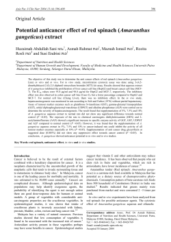


© Copyright 2026