
PARK CITY LECTURES ON EIGENFUNTIONS 1. Introduction
PARK CITY LECTURES ON EIGENFUNTIONS
STEVE ZELDITCH
1. Introduction
These lectures are devoted to nodal geometry of eigenfunctions ϕλ of the Laplacian ∆g of a
Riemannian manifold (M m , g) of dimension m and to the associated problems on Lp norms of
eigenfunctions. The manifolds are generally assumed to be compact, although the problems
can also be posed on non-compact complete Riemannian manifolds. The emphasis of these
lectures is on real analytic Riemannian manifolds. We use real analyticity because the study
of both nodal geometry and Lp norms simplifies when the eigenfunctions are analytically
continued to the complexification of M . Although we emphasize the Laplacian, analogous
2
problems and results exist for Schr¨odinger operators − ~2 ∆g +V for certain potentials V . We
now state state the main results, some classical and some relatively new, that we concentrate
on in these lectures.
2
The study of eigenfunctions of ∆g and − ~2 ∆g + V on Riemannian manifolds is a branch
of harmonic analysis. In these lectures, we emphasize high frequency (or semi-classical)
asymptotics of eigenfunctions and their relations to the global dynamics of the geodesic flow
Gt : S ∗ M → S ∗ M on the unit cosphere bundle
of M . Here and henceforth we identity
Ze3
vectors and covectors using the metric. As in [Ze3] we give the name “Global Harmonic
Analysis” to the use of global wave equation methods to obtain relations between eigenfunction behavior and geodesics. Some of the principal results in semi-classical analysis are
purely local and do not exploit this connection. The relations between geodesics and eigenfunctions belongs to the general correspondence principle between classical and quantum
mechanics.
The correspondence principle has evolved since the origins of quantum mechanSch2
ics [Sch] into
a systematic theory of Semi-Classical
Analysis and Fourier integral operators,
HoI,HoII,HoIII,HoIV
Zw
FORMAT
of which [HoI, HoII, HoIII, HoIV] and [Zw] give systematic presentations; see also §1.13 for
further references. Quantum mechanics provides not only the intuition and techniques for
the study of eigenfunctions, but in large part also provides the motivation. Readers who are
unfamiliar with quantum mechanics
are encouraged
to read the physics literature. Standard
LL
Wei
texts are Landau-Lifschitz [LL] and Weinberg [Wei]. The reader might like to see the images
recently produced by physicists
using quantum microscopes to directly observe nodal sets of
St
excited hydrogen atoms [St].
1.1. The eigenvalue problem on a compact Riemannian manifold. The (negative)
Laplacian ∆g of (M m , g) is the unbounded essentially self-adjoint operator on C0∞ (M ) ⊂
L2 (M, dVg ) defined by the Dirichlet form
Z
D(f ) =
|∇f |2 dVg ,
M
Research partially supported by NSF grant DMS-1206527 .
1
2
STEVE ZELDITCH
where ∇f is the metric gradient vector field and |∇f | is its length in the metric g. Also, dVg
is the volume form of the metric. In terms of the metric Hessian Dd,
∆f = trace Ddf.
In local coordinates,
n
1 X ∂
∂
ij √
∆g = √
g g
,
g i,j=1 ∂xi
∂xj
BGM,Ch
in a standard notation that we assume the reader is familiar with (see e.g. [BGM, Ch] if
not). A more geometric definition uses at each point p an orthomormal basis {ej }m
j=1 of Tp M
and geodesics γj with γj (0) = p, γj0 (0) = ej . Then
X d2
∆f (p) =
f (γj (t)).
2
dt
j
BGM
We refer to [BGM] (G.III.12).
Exercise 1. Let m = 2 and let γ be a geodesic arc on M . Calculate ∆f (s, 0) in Fermi
normal coordinates along γ.
Background: Define Fermi normal coordinates (s, y) along γ by identifying a small ball
bundle of the normal bundle N γ along γ(s) with its image (a tubular neighborhood of γ)
under the normal exponential map, expγ(s) yνγ(s) . Here, νγ(s) is the unit normal at γ(s) (fix
one of the two choices) and expγ(s) yνγ(s) is the unit speed geodesic in the direction νγ(s) of
length y.
The eigenvalue problem is
EIGPROB
(1)
∆g ϕλ = λ2 ϕλ ,
and we assume throughout that ϕλ is L2 -normalized,
Z
2
||ϕλ ||L2 =
|ϕλ |2 dV = 1.
M
EIGPROBb
When M is compact, the spectrum of eigenvalues of the Laplacian is discrete there exists an
orthonormal basis of eigenfunctions. We fix such a basis {ϕj } so that
Z
2
hϕj , ϕk iL2 (M ) :=
ϕj ϕk dVg = δjk
(2)
∆g ϕj = λj ϕj ,
M
If ∂M 6= ∅ we impose Dirichlet or Neumann boundary conditions. Here dVg is the volume
form. When M is compact, the spectrum of ∆g is a discrete set
LAMBDAS
WL
(3)
λ0 = 0 < λ21 ≤ λ22 ≤ · · ·
repeated according to multiplicity. Note that {λj } denote the frequencies, i.e. square roots
of ∆-eigenvalues. We mainly consider the behavior of eigenfuntions in the ‘high frequency’
(or high energy) limit λj → ∞.
The Weyl law asymptotically counts the number of eigenvalues less than λ,
|Bn |
(4)
N (λ) = #{j : λj ≤ λ} =
V ol(M, g)λn + O(λn−1 ).
(2π)n
PARK CITY LECTURES ON EIGENFUNCTIONS
3
Here, |Bn | is the Euclidean volume of the unit ball and V ol(M, g) is the volume of M with
respect
to the metric g. The size of the remainder reflects the measure of closed geodesics
DG,HoIV
[DG, Lpintro
HoIV]. It is
a basic example of global the effect of the global dynamics on the spectrum.
Lp
See §1.12 and §9 for related results on eigenfunctions.
(1) In the aperiodic case where the set of closed geodesics has measure zero, the DuistermaatGuillemin-Ivrii two term Weyl law states
N (λ) = #{j : λj ≤ λ} = cm V ol(M, g) λm + o(λm−1 )
where m = dim M and where cm is a universal constant.
(2) In the periodic case where the geodesic
flow is periodic (Zoll manifolds such as the
√
round sphere), the spectrum of ∆ is a union of eigenvalue clusters CN of the form
2π
β
)(N + ) + µN i , i = 1 . . . dN }
T
4
−1
= 0(N ). The number dN of eigenvalues in CN is a polynomial of degree
CN = {(
with µN i
m − 1.
Remark: The proof that the spectrum is discrete is based on the study of spectral kernels
such as the heat kernel or Green’s function or wave kernel. The standard proof is to show
(whose kernel is the Green’s function, defined on the orthogonal complement of
that ∆−1
g
the constant functions) is a compact self-adjoint operator. By the spectral theory for such
are discrete, of finite multiplicity, and only accumulate
operators, the eigenvalues of ∆−1
g
at 0. Although we concentrate on parametrix constructions for the wave kernel, one can
construct the Hadamard parametrix
for the Green’s function in a similar way. Proofs of the
GSj,DSj,Zw,HoIII
above statements can be found in [GSj, DSj, Zw, HoIII].
The proof of the integrated and pointwise Weyl law are based on wave equation techniques
and Fourier Tauberian theorems. The wave equation techniques mainly involve the construction of parametrices for
the fundamental solution
of the wave equation and the method of
LAGAPP
DG,HoIV
stationary phase. In §13 we review We refer to [DG, HoIV] for detailed background.
1.2. Nodal and critical point sets. The focus of these lectures is on nodal hypersurfaces
RNODAL
(5)
Nϕλ = {x ∈ M : ϕλ (x) = 0}.
The main problems on nodal sets is to determine the hypersurface volume Hm−1 (Nϕλ and
ideally the distribution of nodal sets. Closely related are the other level sets
RLEVEL
(6)
Nϕaj = {x ∈ M : ϕj (x) = a}
and sublevel sets
SUBLEVEL
(7)
{x ∈ M : |ϕj (x)| ≤ a}.
The zero level is distinguished since the symmetry ϕj → −ϕj in the equation preserves the
nodal set.
Remark: Nodals sets belong to individual eigenfunctions. To the author’s knowledge
there
WL PLWL
do not exist any results on averages of nodal sets over the spectrum in the sense of (4)-(40).
4
STEVE ZELDITCH
That is, we do not know of any asymptotic results concerning the functions
X Z
Zf (λ) :=
f dS,
j:λj ≤λ
Nϕj
R
where Nϕ f dS denotes the integral of a continuous function f over the nodal set of ϕj .
j
When the eigenvalues are multiple, the sum Zf depends on the choice of orthonormal basis.
Randomizing by taking Gaussian random combinations of eigenfunctions simplifies nodal
problems profoundly, and are studied in many articles.
One would also like to know the “number” and distribution of critical points,
CRIT
(8)
Cϕj = {x ∈ M : ∇ϕj (x) = 0}.
In fact, the critical point set can be a hypersurface in M , so for counting problems it makes
more sense to count the number of critical values,
CRITV
(9)
Vϕj = {ϕj (x) : ∇ϕj (x) = 0}.
At this time of writing, there exist almost no rigorous upper bounds on the number of critical
values, so we do not spend much space on them here.
The frequency λ of an eigenfunction is a measure of its “complexity” , similar to specifying
the degree of a polynomial, and the high frequency limit is the large complexity limit. A
sequence of eigenfunctions of increasing frequency oscillates more and more rapidly and the
problem is to find its “limit shape”. Sequences of eigenfunctions often behave like “Gaussian random waves” but special ones exhibit highly localized oscillation and concentration
properties.
MOTIVATION
1.3. Motivation. Before stating the problems and results, let us motivate
the study of
EIGPROB
eigenfunctions and their high frequency behavior. The eigenvalue problem (1) arises in many
areas of physics, for example the theory of vibrating membranes. But renewed motivation
to study eigenfunctions comes from quantum
mechanics. As is discussed in any textbook
LL, Wei
on quantum physics or chemistry (see e.g. [LL, Wei]), the Schr¨odinger equation resolves the
problem of how an electron can orbit the nucleus without losing its energy in radiation. The
classical Hamiltonian equations of motion of a particle in phase space are orbits of Hamilton’s
equations
dx
j
∂H
dt = ∂ξj ,
dξj
dt
∂H
= − ∂x
,
j
where the Hamiltonian
1
H(x, ξ) = |ξ|2 + V (x) : T ∗ M → R
2
is the total Newtonian kinetic + potential energy. The idea of Schr¨odinger is to model the
electron by a wave function ϕj which solves the eigenvalue problem
2
EigP
ˆ j := (− ~ ∆ + V )ϕj = Ej (~)ϕj ,
Hϕ
2
ˆ where V is the potential, a multiplication operator on
for the Schr¨odinger operator H,
2
3
L (R ). Here ~ is Planck’s constant, a very small constant. The semi-classical limit ~ → 0
(10)
PARK CITY LECTURES ON EIGENFUNCTIONS
5
is mathematically equivalent to the high frequency limit when V = 0. The time evolution of
an ‘energy state’ is given by
Uth
t
~2
U~ (t)ϕj := e−i ~ (− 2 ∆+V ) ϕj = e−i
(11)
tEj (~)
~
ϕj .
The unitary oprator U~ (t) is often called the propagator. In the Riemannian case with V = 0,
the factors of ~ can be absorbed in the t variable and it suffices to study
U (t) = eit
(12)
√
∆
.
An L2 -normalized energy state ϕj defines a probability amplitude, i.e. its modulus square
is a probability measure with
SQUARE
ME1
(13)
|ϕj (x)|2 dx =
the probability density of finding the particle at x .
According to the physicists,
the observable quantities associated to the energy state are the
SQUARE
probability density (13) and ‘more generally’ the matrix elements
Z
(14)
hAϕj , ϕj i = ϕj (x)Aϕj (x)dV
of observables (A is a self adjoint operator, and in these lectures it is assumed to be a pseudoUth
tEj (~)
differential operator). Under the time evolution (11), the factors of e−i ~ cancel and so
the particle evolves as if “stationary”, i.e. observations of the particle are independent of
the time t.
EigP
Modeling energy states by eigenfunctions (10) resolves the paradox of particles which
are simultaneously in motion and are stationary, but at the cost of replacing the classical
model of particles
following the trajectories of Hamilton’s equations by ‘linear algebra’, i.e.
Uth
evolution by (11). The quantum picture is difficult to visualize or understand intuitively.
Moreover, it is difficult to relate the classical picture of orbits with the quantum picture of
eigenfunctions.
The study of nodal sets was historically motivated in part by the desire to visualize energy
states by finding the points where the quantum particle is least likely to be. In fact, just
recently (at this time or writing)
the nodal sets of the hydrogem atom energy states have
St
become visible to microscopes [St].
LBintro
YAU
1.4. Nodal hypersurface volumes for C ∞ metrics. Let us proceed to the rigorous
results whose proofs we will sketch in these lectures. In the late 700 s, S. T. Yau conjectured
that for general C ∞ (M, g) of any dimension m there exist c1 , C2 depending only on g so
that
(15)
λ . Hm−1 (Nϕλ ) . λ.
Here and below . means that there exists
a constant C independent of λ for which the
YAU
inequality holds. The upper bound of (15) is the analogue for eigenfunctions of the fact that
the hypersurface volume of a real algebraic variety is bounded above by its degree. The lower
bound is specific to eigenfunctions. It is a strong version of the statement that 0 is not an
“exceptional value” of ϕBr
λ . Indeed, a basic result is the following classical result, apparently
due to R. Courant (see [Br])). It is used to obtain lower bounds on volumes of nodal sets:
SMALLBALL
Proposition 1. For any (M, g) there exists a constant A > 0 so that every ball of (M, g)
od radius greater than Aλ contains a nodal point of any eigenfunction ϕλ .
6
STEVE ZELDITCH
PFSMALLBALL
We sketch the proof in §2.2 for completeness, but leave some of the proof as an exercise
to the reader.
YAU
The lower
bound of (15) was proved for all C ∞ metrics for surfaces, i.e. for m = 2 by
Br
metrics in dimensions ≥ 3, the known upper and lower bounds
Br¨
uning [Br]. For general C ∞YAU
are far from the conjecture (15). At present the best lower bound available
for general C ∞
CM
metrics of all dimensions is the following estimate
of Colding-Minicozzi [CM]; a somewhat
SoZ
weaker
bound was proved by Sogge-Zelditch [SoZ]
and the later simplificationSoZa
of the proof
SoZa
CM
[SoZa] turned out to give the same bound as [CM]. We sketch the proof from [SoZa].
CMSZ
Theorem 2.
λ1−
n−1
2
. Hm−1 Nλ ),
SoZ
The original result of [SoZ] HS
is based on lower bounds on the L1 norm of eigenfunctions.
Further work of Hezari-Sogge [HS] shows that the Yau lower bound is correct when one has
||ϕλ ||L1 ≥ C0 for some C0 > 0. It is not known for which (M, g) such an estimate is valid.
At the present time, such lower bounds are obtained from upper bounds on the L4 norm of
ϕj . The study of Lp norms of eigenfunctions is of independent Lp
interest and
we discuss some
Lpintro
recent results which are not directly related to nodal sets In §9 and in §1.12. The study of
Lp norms splits into two very different cases: there exists a critical index pn depending on
the dimension of M , and for p ≥ pn Lpintro
the Lp norms of eigenfunctions are closely related to
the structure of geodesic loops (see §1.12). For 2 ≤ p ≤ pnLpthe Lp norms are governed by
different geodesic properties of (M, g) which we discuss in §9.
We also review an interesting upper bound Dong
due to R. T. Dong and Donnelly-Fefferman in
dimension 2, since the techniques of proof of [Dong] seem capable of further development.
RTDONGth
Theorem 3. For C ∞ (M, g) of dimension 2,
H1 (Nλ ) . λ3/2 .
1.5.
Nodal hypersurface volumes for real analytic (M, g). In 1988, Donnelly-Fefferman
DF
[DF] proved the conjectured bounds for real analytic Riemannian manifolds (possibly with
boundary). We re-state the result as the following
DF
Theorem 4. Let (M, g) be a compact real analytic Riemannian manifold, with or without
boundary. Then
c1 λ . Hm−1 (Zϕλ ) . λ.
DFSECT
We sketch the proof of the upper bound in §10.
1.6. Dynamics of the geodesic or billiard flow. There are two broad classes of results
on nodal sets and other properties of eigenfunctions:
EIGPROB
• Local results which are valid for any local solutionSMALLBALL
of (1), and which often use local
arguments. For instance the proof of Proposition 1 is local.
EIGPROB
• Global results which use that eigenfunctions are global solutions of (1), or that they
satisfy boundary conditions
when ∂M 6= ∅. Thus, they are also satisfy the unitary
Uth
evolution equation (11). For instance the
relation between closed geodesics and the
WL PLWL
remainder term of Weyl’s law is global (4)-(40).
PARK CITY LECTURES ON EIGENFUNCTIONS
7
Global results often exploit the relation between
classical and quantum mechanics, i.e.
EIGPROB
Uth
the relation between the eigenvalue problem (1)-(11) and the geodesic flow. Thus the results often depend on the dynamical properties of the geodesic flow. The relations between
eigenfunctions and the Hamiltonian flow are best established in two extreme cases: (i) where
the Hamiltonian flow is completely integrable on an energy surface, or (ii) where it is ergodic. The extremes are illustrated below in the case of (i) billiards on rotationally invariant
annulus, (ii) chaotic billiards on a cardioid.
A random trajectory in the case of ergodic billiards is uniformly distributed, while all
trajectories are quasi-periodic in the integrable case.
We do not haveHKthe space to review the dynamics of geodesic
flows or other Hamiltonian
Ze,Ze3, Zw
flows. We refer to [HK] for background in dynamics and to [Ze, Ze3, Zw] for relations between
dynamics of geodesic flows and eigenfunctions.
We use the following basic construction: given a measure preserving map (or flow) Φ :
(X, µ) → (T, µ) one can consider the translation operator
UPHI
(16)
UΦ f (x) = Φ∗ f (x) = f (Φ(x)),
RS,HK
sometimes called the Koopman operator or Perron-Frobenius operator (cf. [RS, HK]). It is
a unitary operator on L2 (X, µ) and hence its spectrum lies on the unit circle. Φ is ergodic
if and only if UΦ has the eigenvalue 1 with multiplicity 1, corresponding to the constant
functions.
The geodesic (or billiard) flow is the Hamiltonian flow on T ∗ M generated by the metric
norm Hamiltonian or its square,
X
(17)
H(x, ξ) = |ξ|2g =
g ij ξi ξj .
i,j
√
In PDE one most often uses the H which is homogeneous of degree 1. The geodesic flow
is ergodic when the Hamiltonian flow Φt is ergodic on the level set S ∗ M = {H = 1}.
1.7. Complexifcation
of M and Grauert tubes. The results of Donnelly-Fefferman TheDF
orem 4 in the real analytic case uses in part the analytic continuation of the eigenfunctions
to the complexification of M . One of the themes of these lectures is that nodal problems in
the complex domain are simpler than in the real domain.
A real analytic manifold M always possesses a unique complexification MC generalizing
the complexification of Rm as Cm . The complexification is an open complex manifold in
which M embeds ι : M → MC as a totally real submanifold (Bruhat-Whitney)
The Riemannian metric determines a special kind GS1
of distance function on MC known as
a Grauert tube function. In fact, it is observed in [GS1] that the Grauert tube function
8
STEVE ZELDITCH
p
√
¯ where r2 (x, y) is the
is obtained from the distance function by setting ρ(ζ) = i r2 (ζ, ζ)
squared distance function in a neighborhood of the diagonal in M × M .
√
One defines the Grauert tubes Mτ = {ζ ∈ MC : ρ(ζ) ≤ τ }. There exists a maximal τ0
√
for which ρ is well defined, known as the Grauert tube radius. For τ ≤ τ0 , Mτ is a strictly
pseudo-convex domain in MC . Since (M, g) is real analytic, the exponential map expx tξ
admits an analytic continuation in t and the imaginary time exponential map
EXP
(18)
E : B∗ M → MC ,
E(x, ξ) = expx iξ
is, for small enough , a diffeomorphism from the ball bundle B∗ M of radius in T ∗ M to
¯
the Grauert tube M in MC . We have E ∗ ω = ωT ∗GS1,LS1
M where ω = i∂ ∂ρ and where ωT ∗ M is the
√
canonical symplectic form; and also E ∗ ρ = |ξ| [GS1, LS1]. It follows that E ∗ conjugates
√
the geodesic flow on B ∗ M to the Hamiltonian flow exp tH√ρ of ρ with respect to ω, i.e.
CONJUG
(19)
E(g t (x, ξ)) = exp tΞ√ρ (expx iξ).
In general E only extends as a diffemorphism to a certain maximal radius max . We assume
throughout that < max .
1.8. Equidistribution of nodal sets in the complex domain. One may also consider
the complex nodal sets
(20)
NϕCj = {ζ ∈ M : ϕCj (ζ) = 0},
and the complex critical point sets
(21)
CϕCj = {ζ ∈ M : ∂ϕCj (ζ) = 0}.
Ze5
The following is proved in [Ze5]:
Theorem 5. Assume (M, g) is real analytic and that the geodesic flow of (M, g) is ergodic.
Then for all but a sparse subsequence of λj ,
Z
Z
i
1
√
n−1
f ωg →
f ∂∂ ρ ∧ ωgn−1
λj N C
π M
ϕ
λj
QEDEF
The proof is based on quantum ergodicity of analytic continuation of eigenfunctions to
Grauert tubes and the growth estimates ergodic eigenfunctions satisfy.
We will say that a sequence {ϕjk } of L2 -normalized eigenfunctions is quantum ergodic if
Z
1
(22)
hAϕjk , ϕjk i →
σA dµ, ∀A ∈ Ψ0 (M ).
µ(S ∗ M ) S ∗ M
Here, Ψs (M ) denotes the space of pseudodifferential operators of order s, and dµ denotes
Liouville measure on the unit cosphere bundle S ∗ M of (M, g). More generally, we denote by
dµr the (surface) Liouville measure on ∂Br∗ M , defined by
LIOUVILLE
(23)
dµr =
ωm
on ∂Br∗ M.
d|ξ|g
We also denote by α the canonical action 1-form of T ∗ M .
PARK CITY LECTURES ON EIGENFUNCTIONS
9
1.9. Intersection of nodal sets and real analytic curves on surfaces. To understand
the relation between real and complex zeros, we intersect nodal lines and real analytic on
surfaces dim M = 2. In recent work, intersections of nodal sets and curves have been used
in a variety of articles to obtain upper and lower bounds on nodal points and domains. The
work often is based on restriction theorems for eigenfunctions.
Some of the recent articles on
TZ,TZ2,GRS,JJ,JJ2,Mar,Yo,Po
restriction theorems and/or nodal intersections are [TZ, TZ2, GRS, JJ, JJ2, Mar, Yo, Po].
First we consider a basic upper bound on the number of intersection points:
INTREALBDY
Theorem 6. Let Ω ⊂ R2 be a piecewise analytic domain and let n∂Ω (λj ) be the number of
components of the nodal set of the jth Neumann or Dirichlet eigenfunction which intersect
∂Ω. Then there exists CΩ such that n∂Ω (λj ) ≤ CΩ λj .
In the Dirichlet case, we delete the boundary when considering components of the nodal
set.
INTREALBDY
The method of proof of Theorem 6 generalizes from ∂Ω to a rather large class of real
analytic curves C ⊂ Ω, even when ∂Ω is not real analytic. Let us call a real analytic curve
C a good curve if there exists a constant a > 0 so that for all λj sufficiently large,
GOOD
kϕλj kL2 (∂Ω)
≤ eaλj .
kϕλj kL2 (C)
(24)
Here, the L2 norms refer to the restrictions of the eigenfunction to C and to ∂Ω. The
following result deals with the case where C ⊂ ∂Ω is an interior real-analytic curve. The
real curve C may then be holomorphically continued to a complex curve CC ⊂ C2 obtained
by analytically continuing a real analytic parametrization of C.
GOODTH
Theorem 7. Suppose that Ω ⊂ R2GOOD
is a C ∞ plane domain, and let C ⊂ Ω be a good interior
real analytic curve in the sense of (24). Let n(λj , C) = #Zϕλj ∩ C be the number of intersection points of the nodal set of the j-th Neumann (or Dirichlet) eigenfunction with C. Then
there exists AC,Ω > 0 depending only on C, Ω such that n(λj , C) ≤ AC,Ω λj .
GOODTH
INTREALBDY
The proof of Theorem 7 is somewhat simpler than that of Theorem 6, i.e. good interior
analytic curves are somewhat simpler than the boundary itself. On the other hand, it is clear
that the boundary is good and hard to prove that other curves are good. A JJ
recent paper
of
J. Jung shows that many natural curves in the hyperbolic plane are ‘good’ [JJ]. See also
ElHajT
[ElHajT] for general results on good curves.
The upper bounds are proved by analytically continuing the restricted eigenfunction to
the analytic continuation of the curve. We then give a similar upper bound on complex
zeros. Since real zeros are also complex zeros, we then get an upper bound on complex
zeros. An obvious question is whether the order of magnitude estimate is sharp. Simple
examples in the unit disc show that there are no non-trivial lower bounds on numbers of
intersection points. But when the dynamics is ergodic we can prove an equi-distribution
theorem for nodal intersection points. Ergodicity once again implies that eigenfunctions
oscillate as much as possible and therefore saturate bounds on zeros.
Let γ ⊂ M 2 be a generic geodesic arc on a real analytic Riemannian surface. For small ,
the parametrization of γ may be analytically continued to a strip,
γC : Sτ := {t + iτ ∈ C : |τ | ≤ } → Mτ .
10
STEVE ZELDITCH
Then the eigenfunction restricted to γ is
γC∗ ϕCj (t + iτ ) = ϕj (γC (t + iτ ) on Sτ .
Let
(25)
PLLa
∗ C
Nλγj := {(t + iτ : γH
ϕλj (t + iτ ) = 0}
be the complex zero set of this holomorphic function of one complex variable. Its zeros are
the intersection points.
Then as a current of integration,
2
∗ C
γ
¯
(26)
[Nλj ] = i∂ ∂t+iτ log γ ϕλj (t + iτ ) .
Ze6
The following result is proved in [Ze6]:
NODINT
Theorem 8. Let (M, g) be real analytic with ergodic geodesic flow. Then for generic γ there
exists a subsequence of eigenvalues λjk of density one such that
2
i
∗ C
¯
∂ ∂t+iτ log γ ϕλj (t + iτ ) → δτ =0 ds.
k
πλjk
Thus, intersections of (complexified) nodal sets and geodesics concentrate in the real
domain– and are distributed by arc-length measure on the real geodesic.
The key point is that
1
log |ϕCλj (γ(t + iτ )|2 → |τ |.
k
λj k
Thus, the maximal growth occurs along individual (generic) geodesics.
QCI
1.10. Quantum integrable eigenfunctions. So far, all of the exact asymptotic results we
have discussed assume ergodicity of the geodesic flow. We now give a result in the opposite
dynamical extreme where the geodesic flow is completely integrable. Thus, the phase space
orbits wind around on invariant Lagrangian tori of dimension m = dim M rather than
∗
(almost surely) winding densely around in SM
of dimension 2m − 1. We in fact need to
assume integrability on the quantum level. We only discuss the real analytic case here.
The Laplacian ∆ of a real analytic (M, g) is quantum completely integrable or QCI if there
exist m = dim M first-order analytic pseudo-differential operators P1 , . . . , Pm such that
√
(27)
P1 = ∆, [Pi , Pj ] = 0
and whose symbols (p1 , . . . , pm ) satisfy the non-degeneracy condition
√ dp1 ∧dp2 ∧· · ·∧dpm 6= 0
∗
on a dense open √
set Ω ⊂ T M − 0. We are assuming that P1 = ∆ but it is often simpler
ˆ 1 , . . . , Pm ). Note that the symbols must
to assume that ∆ is some other function H(P
Poisson commute, {pi , pj } = 0, i.e. the associated geodesic flow is completely integrable in
the classical sense that they generate a Hamiltonian Rm action. Simple examples of QCI
Laplacians in dimension two include flat tori, surfaces of revolution, ellipsoids, and Liouville
tori. If one works with Schr¨odinger operators, then there are many further examples such as
the Hydrogen atom, harmonic oscillator, Calogero-Moser Hamiltonian etc.
We denote by {ϕα } an orthonormal basis of joint eigenfunctions,
QCIjt
(28)
Pj ϕα = αj ϕα , hϕα , ϕα0 i = δα,α0 ,
PARK CITY LECTURES ON EIGENFUNCTIONS
11
of the Pj and the joint spectrum of (P1 , . . . , Pm ) by
spectrum
Spec((P1 , . . . , Pm ) = Σ := {~
α := (α1 , ..., αm )} ⊂ Rm .
√
The eigenvalues of ∆ are thus of the form H(~µ) with µ
~ ∈ Σ and the multiplicity of an
eigenvalue is theQCIjt
number of µ
~ with a given value of H(~µ). We refer to the special joint
eigenfunctions (28) as the QCI eigenfunctions. The QI eigenfunctions are complex-valued
and we consider the nodal sets
(29)
Re ϕα = 0, Im ϕα = 0
of their real or imaginary parts.
A completely integrable system is a non-degenerate Hamiltonian Rm actionQCI
on the cotangent bundle T ∗ M of a manifold. The vector of classical symbols of the Pj (27) defines the
moment map
MMP
(30)
P = (p1 , ..., pm ) : T ∗ M − 0 → B ⊂ Rm
of the Hamiltonian action. We assume that the Pj are first order pseudo-differential operators, so that the pj are homogeneous of degree one and thus the image B is a cone. The
level sets P −1 (b) of the moment map consist of a finite union of orbits Hamiltonian flow
PHI
(31)
Φ~t(x, ξ) := exp(t1 Ξp1 ) ◦ ... ◦ exp(t1 Ξpm )(x, ξ), ~t = (t1 , . . . , tm ),
where Ξp denotes the Hamiltonian vector field of p. When compact, the orbits are tori of
dimensions ≤ m. always exist singular levels.
PHI
We say that the Hamiltonian system is toric integrable if the Hamiltonian Rn action (31)
reduces to a Hamilton Tm action where Tm = S 1 ×· · ·×S 1 is the m-torus. Equivalently, if the
integrable system admits global action-angle variables I1 , . . . , Im , θ1 , . . . , θm . By an action
variable is meant a Hamiltonian generating a 2π-periodic Hamiltonian flow. We denote the
moment map by
ical
(32)
I = (I1 , . . . , Im ) : T ∗ M − 0 → B ⊂ Rm .
We assumed above that p1 = |ξ| but with the generators Ij this is not usually the case;
rather there exists a homogeneous function H of degree one so that
|ξ| = H(I1 , . . . , Im ).
The level sets I −1 (b) then consist of a single orbit. On the singular levels, the orbit drops
dimension or equivalent has an isotropy subgroup of positive dimension, much like points on
the divisor at infinity of a toric K¨ahler manifold.
Exercise 2. The geodesic flow of an ellipsoid is not toric integrable. Nor is the geodesic flow
of a “peanut of revolution”. Find a geometric argument that proves that the peanut cannot be
toric integrable. Hint: what kinds of closed geodesics can occur in the toric integrable case?
Toric integrable systems are always toric on the quantum level in the sense that one can
choose generators Iˆ1 , . . . , Iˆm of the algebra of pseudo-differential operators commuting with
∆ whose exponentials generate a unitary representation of Tm on L2 (M ), at least up to
scalars. That is, the joint spectrum is contained in an off-set of a conic subset Λ of a lattice,
(33)
Sp(Iˆ1 , . . . , Iˆm ) = Λ + ν ⊂ Zm + ν,
12
STEVE ZELDITCH
where ν ∈ (Z/4)m is a Maslov index. For instance in the case of the standard S 2 one can
choose generators whose spectrum is the set {(m, n + 12 ) : −n ≤ m ≤ n, n ≥ 0}.
Semiclassical limits are taken along ladders in the joint spectrum. In the case of quantum
torus actions, we define rational ladders by
(34)
Lα = Rα + ν, (α ∈ Λ).
Thus, rational rays consist of multiples of a given lattice point.
We refer to a ladder as a regular ladder if P −1 (α) is a regular level, and as a singular
ladder if P −1 (α) is a singular level. For simplicity, we only consider limit distribution along
ladders for regular levels. We transfer the moment map I to M by
(35)
I : M → Rn , I = I ◦ E −1 .
The eigenfunctions ϕα admit holomorphic extensions ϕCα to a certain Grauert tube M
independent of α. We note that ϕα is normalized to have L2 -norm equal to 1 but is only
defined up to a unit complex number. Since it is not unique, we consider ϕCα (z)ϕCα (y) where
y is fixed and z varies. We then consider the analytic continuations of the real and imaginary
parts,
C C
Re ϕα (x)ϕα (y) ,
Im ϕα (x)ϕα (y) .
RE
ubt
LAMBDAALPHA
In the case of a QCI system, ϕα (x) = ϕ−α (x) for x ∈ M, hence
C
1
(36)
Re ϕα (·)ϕα (y) (z) = (ϕCα (z)ϕC−α (y) + ϕC−α (z)ϕCα (y)).
2
To illustrate the notation, in the case of Rn /Zn we have ϕα (x) = eihα,xi , Re ϕα (x)ϕα (y) =
C
coshα, x − yi and Re ϕα (·)ϕα (y) (z) = coshα, z − yi. In this example it is natural to set
y = 0.
As discussed above, the key problem in finding the limit distribution of nodal sets in the
complex domain is to determine the exponential
growth rate of the complexified eigenfuncRE
tions. In the QCI case, the growth rates of (36) depend on the ladder Lα . We therefore
define
√
1
C
ρα (z) := limk→∞ kH(α) log |ϕkα (z)|
(37)
C
.
1
C
C
C
uα (z; y) := limk→∞ kH(α) log ϕkα (z)ϕkα (y) + ϕ−kα (z)ϕ−kα (y)
√
The
zero set of ρα is a real hypersurface in M known as the Anti-Stokes hypersurface (see
AntiS
§??.)
ϕC (z)ϕC (y)
}∞
To determine the exponential growth asymptotics of the sequence { kα||ϕC ||kα
2
k=1 , we
α find a convenient complex oscillatory integral expression for it and then use the method of
complex stationary phase. Since the ladder Lα is fixed, there is a distinguised level set of
the moment map in each ∂M .
Definition 9. We put
α
• Λα := I −1 ( H(α)
) ⊂ T ∗ M \0.
α
• Λα = E(Λα ) = I−1 ( H(α)
) ⊂ ∂M .
PARK CITY LECTURES ON EIGENFUNCTIONS
13
ALL
These level sets are torus orbits and we view them as the classically allowed set (see §??
e ~y = z in this
for background). The main point is that there exists a real ~t ∈ Tm so that Φ
t
ϕC (z)ϕC (y)
case, and it is then straightforward to determine the asymptotics of { kα||ϕC ||kα
}∞
2
k=1 when
α z, y ∈ Λ .
The main complication is that for z ∈
/ Λα , i.e. in the classically forbidden region, there does
not exist a critical point of the complex oscillatory integral on the contour of integration.
We therefore must locate the dominant critical point in the complexification TCm × (M )C
of the contour, where (M )C is the complexification of the Grauert tube (viewed as a real
manifold). We further must analytically continue the torus action to this complexification.
It turns out to be important to distinguish between the analytic continuation of orbits to
complex time on M and the analytic continuation of the group action to (M )C To explain
this and to state the results, we need to introduce some further notation.
dcalz
Definition 10. We denote by Γz : Tm → M the orbit Γz (~t) of a point z ∈ M under Tm .
We further denote by Dz ⊂ Tm
C the maximal domain of analytic continuation of Γz ,
Γz : Dz → M .
Given two regular points (y, z) ∈ ∂Mreg × ∂Mreg there exists a unique ((~t + i~τ )(z, y) ∈ Tm
C
so that Γy (~t + i~τ ) = z.
TT
Definition 11. We define two complex travel times with respect to the complexified torus
action:
• Given z ∈ ∂M there exists a unique imaginary time ~τ (z, α) ∈ Rm so that
Γz (exp i~τ (z, α)) ∈ Λα ⊂ ∂M .
α
• Given a second point y ∈ ∂M , satisfying I (y) = H(α)
, there exists a unique complex
time ~t(z, α, y) + iτ (z, α, y) so that
Γz (exp ~t(z, y) + iτ (z, y)) = y.
The imaginary time ~τ (z, α)) is the travel time from z to Λα . Note that if we move a point
on Λα , it changes the travel time by a real vector and does not change the imaginary part.
On the other hand, ~t(z, y) + iτ (z, y) is the complex travel time from z to y.
QCIGR
Theorem 12. Let (M, g) be a real analytic Riemannian manifold with quantum torus integrable Laplacian, and let {ϕkα } be a regular ladder of L2 -normalized joint eigenfunctions.
Let z ∈ ∂M and let y ∈ I−1 (α). Then,
√
√
1
α
ρα (z) = 2 h H(α) , ~τ (z, α)i + ρ(z)
√
√
α
α
i + ρ(z), − 12 h~τ (z, −α, y), H(α)
i + ρ(z)}
uα (z) = max{ 21 h~τ (z, α, y), H(α)
√
We note that ρ is the maximal exponent of growth of eigenfunctions, so we must have
√
√
√
√
√
ρα (z) ≤ ρ(z). Note that ρMAINPROPintro
= − ρα and uα = | ρα |
−α
Combining with Proposition 8.1 gives our main result,
14
RESULT
STEVE ZELDITCH
Corollary 13. Let NαC be the complex nodal set of Re ϕα . Then for a regular ladder
Lα = {kα, k ∈ Z+ }, uα is well-defined and the limit distribution of the nodal set currents
along the ladder is given by
Z
Z
α
1
i
i ¯ √
m−1
m−1
lim
i + ρ(z) .
f ωρ
→
f ωρ ∧ ∂ ∂ h~τ (z, α, y),
k→∞ k||α|| N C
π M
π
H(α)
kα
The restriction to regular ladders is not just technical. The methods and results
are differEXAMPLES
ent for singular levels, as illustrated by highest weight spherical harmonics (§3.6). They have
unusual growth and decay behavior in both the real and complex domain. Eigenfunctions
associated to singular levels are important and we plan to study them in a future article.
Note that ϕCα has no complex zeros if and only if h~τ (z, αi is a harmonic function.
1.11. Example: Flat torus. Flat tori Rn /L are quantum integrable with Iˆj = ∂x∂ j . The
~
QI joint eigenfunctions are of course the exponentials eihλ,xi where ~λ ∈ L∗ , the dual lattice
to L. The corresponding real eigenfunctions are sinhx, ~λi, coshx, ~λi, and their analytic continuations are sinhζ, λi, coshζ, λi. All of their complex zeros ζ = x + iξ mod L are real and
satisfy
FLATZ
(38)
sinhx + iξ, ~λi = 0 ⇐⇒ hx, ~λi ∈ πZ, hξ, ~λi = 0.
In the case of Rn /Z n , the classically allowed region for eihα,xi is the entire torus. Upon
analytic continuation we see that along a ray of lattice points, eihkα,x+iξi is exponentially
growing when hξ, αi < 0 and is exponentially decaying where hξ, αi > 0. Thus the real
hypersurface {x + iξ ∈ (Cn /L) : hξ, αi = 0} is the boundary between the two regimes and is
thus the anti-Stokes surface
ASα = {z : hIm z, αi = 0}.
The level set of the moment map is the Lagrangian torus ξ =
α
maximum growth rate. With y = |α|
,
τ (z, α) = Im z − α
,
|α|
τ (z, α, `
,
|`|
where ϕCα attains its
α
α
) = Im z − ,
|α|
|α|
so that
√
α
α
α
ρα (z) = hIm z − |α| , |α| i + = hIm z, |α| i,
u (z) = max{hIm z − α , α i + 2, hIm z + α , − α i + 2} = |hIm z, α i|.
α
|α| |α|
|α|
|α|
|α|
The nodal set of the complexified real part is given by
coshkα, x + iξi = 0 ⇐⇒ hξ, αi = 0,
khα, xi = π/2 mod 2π,
so that the limit nodal set lies in ASα and is uniformly distributed on it.
The explicitly computable examples like the flat torus or sphere are not representative
since the torus acts by holomorphic maps in these cases. The holomorphic maps necessarily
extend to the zero section and must be lifts of isometries of the base.
PARK CITY LECTURES ON EIGENFUNCTIONS
15
LBintro
Lpintro
SPECFUN
1.12. Lp norms of eigenfunctions. In §1.4 we mentioned that lower bounds on Hn−1 (Nϕλ
are related to lower bounds on ||ϕλ ||L1 and to upper bounds on ||ϕλ ||Lp for certain p. Such
Lp bounds
are interesting for all p and depend on the shapes of the eigenfunctions.
WL
In (4) we stated the Weyl law on the number of eigenvalues. There also exists a pointwise
local Weyl law which is relevant to the pointwise behavior of eigenfunctions. The pointwise
spectral function along the diagonal is defined by
X
(39)
E(λ, x, x) = N (λ, x) :=
|ϕj (x)|2 .
λj ≤λ
The pointwise Weyl law asserts tht
PLWL
COSINE
(40)
N (λ, x) =
1
|B n |λn + R(λ, x),
(2π)n
where R(λ, x) = O(λn−1 ) uniformly in x. These results are proved by studying the cosine
transform
X
cos tλj |ϕj (x)|2 ,
(41)
E(t, x, x) =
λj ≤λ
03
which is the fundamental (even) solution of the
wave equation restricted to the diagonal.
WAVEAPP
Background on the wave equation is given in §12.
1
n n
We note that the Weyl asymptote (2π)
is continuous, while the spectral function
n |B |λ
SPECFUN
(39) is piecewise constant with jumps at the eigenvalues λj . Hence the remainder must jump
at an eigenvalue λ, i.e.
X
|ϕj (x)|2 = O(λn−1 ).
(42)
R(λ, x) − R(λ − 0, x) =
j:λj =λ
on any compact Riemannian manifold. It follows immediately that
n−1
MAXSUP
(43)
sup |ϕj | . λj 2 .
M
Lambdap
There exist (M, g) for which this estimate is sharp, such as the standard spheres. However,
it is very rarely sharp and the actual size of the sup-norms and otherSoZ
Lp norms of eigenfunctions is another
interesting problem in global harmonic analysis. In [SoZ] it is proved that if
MAXSUP
the bound (43) is achieved by some sequence of eigenfunctions, then there must exist a “partial blow-down point” or self-focal point p where a positive measure of directions ω ∈ Sp∗ M
so that the geodesic with initial value (p, ω) returns to p at some time T (p, ω). Recently the
authors
have improved the result in the real analytic case, and we sketch the new result in
Lp
§9.
To state it, we need some further notation and terminology. We only consider real analytic
metrics for the sake of simplicity. We call a point p a self-focal point or ablow-down point
if there exists a time T (p) so that expp T (p)ω = p for all ω ∈ Sp∗ M . Such a point is selfconjugate in a very strong sense. In terms of symplectic geometry, the flowout manifold
[
(44)
Λp =
Gt Sp∗ M
0≤t≤T (p)
16
STEVE ZELDITCH
is an embedded Lagrangian submanifold of S ∗ M whose projection
π : Λp → M
STZ
has a “blow-down singuarity” at t = 0, t = T (p) (see[STZ]). Focal points come in two basic
kinds, depending on the first return map
Phix
(45)
Φp : Sp∗ M → Sp∗ M,
0
Φp (ξ) := γp,ξ
(T (p)),
where γp,ξ is the geodesic defined by the initial data (p, ξ) ∈ Sx∗ M . We say that p is a pole if
Φp = Id : Sp∗ M → Sp∗ M.
On the other hand, it is possible that Φp = Id only on a codimension one set in Sp∗ M . We
call such a Φp twisted.
Examples of poles are the poles of a surface of revolution (in which case all geodesic loops
at x0 are smoothly closed). Examples of self-focal points with fully twisted return map are
the four umbilic points of two-dimensional tri-axial ellipsoids, from which all geodesics loop
back at time 2π but are almost never smoothly closed. The only smoothly closed directions
are the geodesic (and its time reversal) defined by the middle length ‘equator’.
UPHI
UX
At a self-focal point we have a kind of analogue of (16) but not on S ∗ M but just on Sp∗ M .
We define the Perron-Frobenius operator at a self-focal point by
p
(46)
Ux : L2 (Sx∗ M, dµx ) → L2 (Sx∗ M, dµx ), Ux f (ξ) := f (Φx (ξ)) Jx (ξ).
Here, Jx is the Jacobian of the map Φx , i.e. Φ∗x |dξ| = Jx (ξ)|dξ|.
The new result of C.D. Sogge and the author is the following:
TL
Theorem 14. If (M, g) is real analytic and has maximal eigenfunction growth, then it possesses a self-focal point whose first return map Φp has an invariant L2 function in L2 (Sp∗ M ).
Equivalently, it has an L1 invariant measure in the class of the Euclidean volume density µp
on Sp∗ M .
For instance, the twisted first return map at an umbilic point of an ellipsoid has no such
finite invariant measure. Rather it has two fixed points, one of which is a source and one a
sink, and the only finite invariant measures are delta-functions at the fixed points. It also
has an infinite invariant
measure on the complement of the fixed points, similar to dx
on R+ .
x
SoZ,STZ,SoZ2
The results of [SoZ, STZ, SoZ2] are stated for the L∞ norm but the
same
results
are
true
for
Lp
p
L norms above a critical index pm depending on the dimension (§9). The analogous problem
for lower Lp norms is of equal interest, but the geometry of the extremals changes from
analogues of zonal harmonics to analogoues of Gaussian beams or highest weight harmonics.
Lp
For the lower Lp norms there are also several new developments which are discussed in §9.
FORMAT
1.13. Format of these lectures and references to the literature. In keeping with the
format of the Park City summer school, various details of the proof are given as Exercises
for the reader. The “details” are intended to be stimulating and fundamental, rather than
the tedious and routine aspects of proofs often left to readers in textbooks. As a result, the
exercises vary widely in difficulty and amount of background assumed. Problems labelled
Problems are not exercises; they are problems whose solutions are not currently known.
PARK CITY LECTURES ON EIGENFUNCTIONS
17
The technical backbone of the semi-classical analysis of eigenfunctions consists of wave
equation methods combined with the machinery of Fourier integral operators and Pseudodifferential operators. We do not have time to review this theory. The main
√ results we
need are the construction
of parametrices for the ‘propagator’ E(t) = cos t ∆ and the
√
Poisson kernel√exp −τ ∆. We also need Fourier analysis to construct approximate spectral
projections ρ( ∆ − λ) and to prove Tauberian theorems relating smooth expansions and
cutoffs.
GSj, DSj, D2, GSt1,GSt2, Sogb, Sogb2, Zw
The books [GSj, DSj, D2, GS2, GSt2, Sogb, Sogb2, Zw] give textbook treatments of the
semi-classical methods with applications to spectral asymptotics. Somewhat more classical
background
on the wave equation with many explicit formulae in model cases can be found
TI,TII
in
[TI,
TII].
General
spectral theory and the relevant functional analysis can also be found in
RS
HoI,HoII,HoIII,HoIV
[RS]. The series [HoI, HoII, HoIII, HoIV] gives a systematic presentation of Fourier
integral
HoI
operator theory: stationary phase and Tauberian
theorems
can
be
found
in
[HoI],
Weyl’s
HoIII,HoIV
law and
spectral asymptotics can be found in [HoIII, HoIV].
Ze0
In [Ze0] the author gives a more systematic presentation Ze,Ze2,Ze3
of results on nodal sets, Lp
norms and other aspects of eigenfunctions. Earlier surveys [Ze, Ze2,
Ze3] survey
related
HL
Sogb2
material. Other
monographs
on
∆-eigenfunctions
can
be
found
in
[HL]
and
[Sogb2].
The
HL
methods of [HL] mainly involve the local harmonic analysis of eigenfunctions and rely more
on classical ellipticSogb2
estimates, on frequency functions and of one-variable complex analysis.
The exposition in [Sogb2] is close to the one given
here but does not extend to the recent
Ze0
results that we highlight in these lectures and in [Ze0].
Acknowledgements Many of the results discussed in these lectures is joint work with C.
D. Sogge and/or John. A. Toth. Some of the work in progress is also with B. Hanin and P.
Zhou. We also thank E. Potash for his comments on earlier versions.
2. Foundational results on nodal sets
FOUND
The nodal domains of an eigenfunction are the connected components of M \Nϕλ . In the
case of a domain with boundary and Dirichlet boundary conditions, the nodal set is defined
by taking the closure of the zero set in M \∂M .
The eigenfunction is either positive or negative in each nodal domain and changes sign
as the nodal set is crossed from one domain to an adjacentH domain. Thus the set of nodal
domains can be given the structure of a bi-partite graph [H]. Since the eigenfunction has
one sign in each nodal domain, it is the ground state eigenfunction with Dirichlet boundary
conditions in each nodal domain.
In the case of domains Ω ⊂ Rn (with the Euclidean metric), the Faber-Krahn inequality
states that the lowest eigenvalue (ground state eigenvalue, bass note) λ1 (Ω) for the Dirichlet
problem has the lower bound,
FK1
(47)
2
2
λ1 (Ω) ≥ |Ω|− n Cnn j n−2 ,
2
n
π2
Γ( n
+1)
2
where |Ω is the Euclidean volume of Ω, Cn =
is the volume of the unit ball in Rn and
where jm,1 is the first positive zero of the Bessel function Jm . That is, among all domains of
a fixed volume the unit ball has the lowest bass note.
18
STEVE ZELDITCH
2.1. Vanishing order and scaling near zeros. By the vanishing order ν(u, a) of u at
a is meant the largest positive integer such that Dα u(a) = 0 for all |α| ≤ ν. A unique
continuation theorem shows that the vanishing order of an eigenfunction at each zero is
finite. The following estimate is a quantitative version of this fact.
DF
VO
Lin
H
Theorem 2.1. (see [DF]; [Lin] Proposition 1.2 and Corollary 1.4; and [H] Theorem 2.1.8.)
Suppose that M is compact and of dimension n. Then there exist constants C(n), C2 (n)
depending only on the dimension such that the the vanishing order ν(u, a) of u at a ∈
M satisfies ν(u, a) ≤ C(n) N (0, 1) + C2 (n) for all a ∈ B1/4 (0). In the case of a global
eigenfunction, ν(ϕλ , a) ≤ C(M, g)λ.
Highest weight spherical harmonics Cn (x1 + ix2 )N on S 2 are examples which vanish at the
maximal order of vanishing at the poles x1 = x2 = 0, x3 = ±1.
The following Bers scaling rule extracts the leading term in the Taylor expansion of the
eigenfunction around a zero:
Bers,HW2
0
[Bers, HW2] Assume that ϕλ vanishes to order k at x0 . Let ϕλ (x) = ϕxk0 (x) + ϕxk+1
+ ···
∞
denote the C Taylor expansion of ϕλ into homogeneous terms in normal coordinates x
centered at x0 . Then ϕxk0 (x) is a Euclidean harmonic homogeneous polynomial of degree k.
SCALING
PFSMALLBALL
To prove this, one substitutes the homogeneous expansion into the equation ∆ϕλ = λ2 ϕλ
and rescales x → λx, i.e. one applies the dilation operator
u
(48)
Dλx0 ϕλ (u) = ϕ(x0 + ).
λ
The rescaled eigenfunction is an eigenfunction of the locally rescaled Laplacian
n
X
∂2
x0 −1
x0
−2 x0
(49)
∆λ := λ Dλ ∆g (Dλ ) =
+ ···
∂u2j
j=1
in Riemannian normal coordinates u at x0 but now with eigenvalue 1,
Dλx0 ∆g (Dλx0 )−1 ϕ(x0 + λu ) = λ2 ϕ(x0 + λu )
(50)
=⇒ ∆xλ0 ϕ(x0 + λu ) = ϕ(x0 + λu ).
Since ϕ(x0 + λu ) is, modulo lower order terms, an eigenfunction of a standard flat Laplacian
on Rn , it behaves near a zero as a sum of homogeneous Euclidean harmonic polynomials.
The Bers scaling is used by S.Y. Cheng (see also earlier results of Hartman-Wintner
HW,Ch1,Ch2
[HW, Ch1, Ch2]) to prove that at a singular point of ϕλ in dimension two, the nodal line
branches
in k curves at x0 with equal angles between the curves. For further applications,
Bes
see [Bes].
Question Is there any useful scaling behavior of ϕλ around its critical points?
SMALLBALL
2.2. Proof of Proposition 1. The proofs are based on rescaling the eigenvalue problem
in small balls.
Proof. Fix x0 , r and consider B(x0 , r). If ϕλ has no zeros in B(x0 , r), then B(x0 , r) ⊂ Dj;λ
must be contained in the interior of a nodal domain Dj;λ of ϕλ . Now λ2 = λ21 (Dj;λ ) where
λ21 (Dj;λ ) is the smallest Dirichlet eigenvalue for the nodal domain. By domain monotonicity
of the lowest Dirichlet eigenvalue (i.e. λ1 (Ω) decreases as Ω increases), λ2 ≤ λ21 (Dj;λ ) ≤
PARK CITY LECTURES ON EIGENFUNCTIONS
19
λ21 (B(x0 , r)). To complete the proof we show that λ21 (B(x0 , r)) ≤ rC2 where C depends only
on the metric. This is proved by comparing λ21 (B(x0 , r)) for the metric g with the lowest
Dirichlet Eigenvalue λ21 (B(x0 , cr); g0 ) for the Euclidean ball B(x0 , cr; g0 ) centered at x0 of
radius cr with Euclidean metric g0 equal to g with coefficients frozen at x0 ; c is chosen so that
B(x0 , cr; g0 ) ⊂ B(x0 , r, g). Again by domain Rmonotonicity, λ21 (B(x0 , r, g)) ≤ λ21 (B(x0 , cr; g))
|df |2 dV
for c < 1. By comparing Rayleigh quotients RΩ f 2 dVgg one easily sees that λ21 (B(x0 , cr; g)) ≤
Ω
Cλ21 (B(x0 , cr; g0 )) for some C depending only on the metric. But by explicit calculation with
Bessel functions, λ21 (B(x0 , cr; g0 )) ≤ rC2 . Thus, λ2 ≤ rC2 .
Ch
For background we refer to [Ch].
HL
2.3. A second proof. Another proof is given in [HL]: Let ur denote the ground state
Dirichlet eigenfunction for B(x0 , r). Then ur > 0 on the interior of B(x0 , r). If B(x0 , r) ⊂
Dj;λ then also ϕλ > 0 in B(x0 , r). Hence the ratio ϕuλr is smooth and non-negative, vanishes
only on ∂B(x0 , r), and must have its maximum at a point y in the interior of B(x0 , r). At
this point (recalling that our ∆ is minus the sum of squares),
ur
ur
∇
(y) = 0, −∆
(y) ≤ 0,
ϕλ
ϕλ
so at y,
ur
ϕλ ∆ur − ur ∆ϕλ
(λ21 (B(x0 , r)) − λ2 )ϕλ ur
0 ≥ −∆
=−
=
−
.
ϕλ
ϕ2λ
ϕ2λ
Since ϕϕλ2ur > 0, this is possible only if λ1 (B(x0 , r)) ≥ λ.
λ
To complete the proof we note that if r = Aλ then the metric is essentially Euclidean. We
rescale the ball by x → λx (with coordinates centered at x0 ) and then obtain an essentially
Euclidean ball of radius r. Then λ1 (B(x0 , λr ) = λλ1 Bg0 (x0 , r). Therefore we only need to
choose r so that λ1 Bg0 (x0 , r) = 1.
2.4. Rectifiability of the nodal set. We recall that the nodal set of an eigenfunction ϕλ
is its zero set. When zero is a regular value
of ϕλ the nodal set isBae
a smooth hypersurface.
U
This is a generic property of eigenfunctions [U]. It is pointed out in [Bae] that eigenfunctions
can always be locally represented in the form
!
k−1
X
ϕλ (x) = v(x) xk1 +
xj1 uj (x0 ) ,
j=0
0
in suitable coordinates (x1 , x ) near p, where ϕλ vanishes to order k at p, where uj (x0 ) vanishes
to order k − j at x0 = 0, and where v(x) 6= 0 in a ball around p. It follows that the nodal
set is always countably n − 1 rectifiable when dim M = n.
LB
3. Lower bounds for Hm−1 (Nλ ) for C ∞ metrics
CM,SoZ,SoZa,HS,HW
In this section we review the lower bounds on Hn−1 (Zϕλ ) from [CM, SoZ, SoZa, HS, HW].
Here
Z
n−1
H (Zϕλ ) =
dS
Zϕλ
20
STEVE ZELDITCH
is the Riemannian surface measure, where dS denotes the Riemannian volume element on
the nodal set, i.e. the insert iotan dVg of the unit normal into the volume form of (M, g).
The main result is:
DONGLB
Theorem 3.1. Let (M, g) be a C ∞ Riemannian manifold. Then there exists a constant C
independent of λ such that
n−1
Cλ1− 2 ≤ Hn−1 (Zϕλ ).
DONGLB
SoZ,SoZa
WeSoZ
sketch the proof of Theorem 3.1Dong
from [SoZ, SoZa]. The starting point is an identity
from [SoZ] (inspired by an identity in [Dong]):
DONGPROP
1
Proposition 3.2. For any f ∈ C 2 (M ),
Z
Z
2
|ϕλ | (∆g + λ )f dVg = 2
(51)
M
|∇g ϕλ | f dS,
Zϕλ
When f ≡ 1 we obtain
DONGCOR
1a
Corollary 3.3.
2
(52)
Z
Z
|ϕλ | dVg = 2
λ
M
|∇g ϕλ | f dS,
Zϕλ
Exercise 3. Prove this identity by decomposing M into a union of nodal domains.
DONGLB
DONGCOR
The lower bound of Theorem 3.1 follows from the identity in Corollary 3.3 and the following
lemma:
lem
Lemma 3.4. If λ > 0 then
4.0
(53)
EST
k∇g ϕλ kL∞ (M ) . λ1+
n−1
2
kϕλ kL1 (M )
Here, A(λ) . B(λ) means that there exists a constant independent of λ so that A(λ) ≤
CB(λ).
lem
DONGCOR
By Lemma 3.4 and Corollary 3.3, we have
R
R
λ2 M |ϕλ | dV = 2 Zλ |∇g ϕλ |g dS 6 2|Zλ | k∇g ϕλ kL∞ (M )
(54)
n−1
. 2|Zλ | λ1+ 2 kϕλ kL1 (M ) .
DONGLB
Thus Theorem 3.1 follows from the somewhat curious cancellation of ||ϕλ ||L1 from the two
sides of the inequality.
lem
3.1. Proof of Lemma 3.4.
HATRHO
Proof. The main idea is to construct a designer reproducing kernel for ϕλ of the form
Z ∞
√
p
(55)
ρˆ(λ − −∆g )f =
ρ(t)e−itλ eit −∆g f dt,
−∞
with ρ ∈
C0∞ (R).
PARK CITY LECTURES ON EIGENFUNCTIONS
21
HATRHO
Exercise 4. Prove that (55) has the spectral expansion,
5.0
(56)
χλ f =
∞
X
ρˆ(λ − λj )Ej f,
j=0
where Ej f is the projection of f onto the λj - eigenspace of
reproduces ϕλ if ρˆ(0) = 1.
p
HATRHO
−∆g . Conclude that (55)
We denote the kernel of χλ by Kλ (x, y), i.e.
Z
χλ f (x) =
Kλ (x, y)f (y)dV (y), (f ∈ C(M )).
M
Assuming ρˆ(0) = 1, then
Z
Kλ (x, y)ϕλ (y)dV (y) = ϕλ (x).
lem
M
To obtain Lemma 3.4, we choose ρ so that the reproducing kernel Kλ (x, y) is uniformly
n−1
bounded by λ 2 on the diagonal as λ → +∞. It suffices to choose ρ so that ρ(t) = 0 for
|t| ∈
/ [ε/2, ε], with ε > 0 less than the injectivity radius of (M, g).
Exercise 5. Prove that
Ka
(57)
Kλ (x, y) = λ
n−1
2
aλ (x, y)eiλr(x,y) ,
where aλ (x, y) is bounded with bounded derivatives in (x, y) and where r(x, y) is the Riemannian distance between points. This WKB formula for Kλ (x, y) is known as a parametrix.
(Hint: use the Hadamard parametrix) and stationary phase).
Ka
It follows from (57) that
K
(58)
|∇g Kλ (x, y)| 6 Cλ1+
n−1
2
,
and therefore,
(59)
R
supx∈M |∇g χλ f (x)| = supx f (y) ∇g Kλ (x, y) dV 6 ∇g Kλ (x, y) ∞
kf kL1
L (M ×M )
6 Cλ1+
lem
n−1
2
kf kL1 .
To complete the proof of Lemma 3.4, we set f = ϕλ and use that χλ ϕλ = ϕλ .
We view Kλ (x, y) as a designer reproducing kernel, because it is much
smaller on the
P
diagonal than kernels of the spectral projection operators E[λ,λ+1] = j:λj ∈[λ,λ+1] Ej . The
restriction onSoZa
the support of ρ removes the big singularity on the diagonal at t = 0. As
discussed in [SoZa], it is possible to use this kernel because we only need it to reproduce one
eigenfunction and not a whole spectral interval of eigenfunctions.
22
STEVE ZELDITCH
DONGPROP
HS
3.2. Modifications. Hezari-Sogge modified the proof Proposition 3.2 in [HS] to prove
HS
2
Theorem 3.5. For any C ∞ compact Riemannian manifold, the L2 -normalized eigenfunctions satisfy
Hn−1 (Zϕλ ) ≥ C λ ||ϕλ ||2L1 .
They first apply the Schwarz inequality to get
Z
2
(60)
λ
|ϕλ | dVg 6 2(Hn−1 (Zϕλ ))1/2
!1/2
Z
M
2
|∇g ϕλ | dS
.
Zϕλ
They then use the test function
6
f = 1 + λ2 ϕ2λ + |∇g ϕλ |2g
(61)
12
DONGPROP
in Proposition 3.2 to show that
Z
|∇g ϕλ |2 dS ≤ λ3 .
(62)
Zϕλ
Ar
See also [Ar] for the generalization to the nodal bounds to Dirichlet and Neumann eigenfunctions of HS
bounded domains.
Theorem 3.5 shows that Yau’s conjectured lower bound would follow for a sequence of
eigenfunctions satisfying ||ϕλ ||L1 ≥ C > 0 for some positive constant C.
LBL1
CS
3.3. Lower bounds on L1 norms of eigenfunctions. The following universal lower
bound is optimal as (M, g) ranges over all compact Riemannian manifolds.
Proposition 15. For any (M, g) and any L2 -normalized eigenfunction, ||ϕλ ||L1 ≥ Cg λ−
n−1
4
.
Remark: There are few results on L1 norms of eigenfunctions. The reason is probably that
|ϕλ |2 dV is the natural probability measure associated to eigenfunctions. It is straightforward
to show that the expected L1 norm of random L2 -normalized spherical harmonics of degree
N and their generalizations to any (M, g) is a positive constant CN with a uniform positive
lower bound. One expects eigenfunctions in the ergodic case to have the same behavior.
Problem 1. A difficult but interesting problem would be to show that ||ϕλ ||L1 ≥ C0 > 0 on
a compact hyperbolic manifold. A partial result in this direction would be useful.
3.4. Dong’s upper bound. Let (M, g) be a compact C ∞ Riemannian manifold of dimesion
n, let ϕλ be an L2 -normalized eigenfunction of the Laplacian,
∆ϕλ = −λ2 ϕλ ,
Let
q
q = |∇ϕ|2 + λ2 ϕ2 .
(63)
D
MAINDONG
In Theorem 2.2 of [D], R. T. Dong proves the bound
Z
√
1
n−1
(64)
H (N ∩ Ω) ≤
|∇ log q| + nvol(Ω)λ + vol(∂Ω).
2 Ω
PARK CITY LECTURES ON EIGENFUNCTIONS
23
He also proves (Theorem 3.3) that on a surface,
Deltaq
∆ log q ≥ −λ + 2 min(K, 0) + 4π
(65)
X
(ki − 1)δpi ,
i
where {pi } are the singular points and ki is the order of pi . In Dong’s notation,
λMAINDONG
> 0. Using
Deltaq
a weak Harnack inequality, Dong shows (loc. cit. Theorem 4.2) how (65) and (64) combine
to produce the upper bound H1 (N ∩ Ω) ≤ λ3/2 in dimension 2.
Problem 2. To what extent can one generalize these estimates to higher dimensions?
3.5. Other level sets. Although nodal sets are special, it is of interest to bound the Hausx
dorff surface measure of any level set Nϕcλ := {ϕλ = c}. Let sgn (x) = |x|
.
BOUNDSc
Proposition 3.6. For any C ∞ Riemannian manifold, and any f ∈ C(M ) we have,
Z
DONGTYPEc
2
2
f (∆ + λ ) |ϕλ − c| dV + λ c
(66)
Z
Z
f sgn (ϕλ − c)dV = 2
f |∇ϕλ |dS.
Nϕc
M
λ
This identity has similar implications for Hn−1 (Nϕcλ ) and for the equidistribution of level
sets.
cintro
Corollary 3.7. For c ∈ R
λ
2
|∇ϕλ |dS.
ϕλ dV =
ϕλ >c
c
Z
Z
Nϕc
λ
One can obtain lower bounds on Hn−1 (Nϕcλ ) as in the case of nodal sets. However the
integrals of |ϕλ | no longer cancel out. The numerator is smaller since one only integrates
over {ϕλ ≥ c}. Indeed, Hn−1 (Nϕcλ ) must tend to zero as c tends to the maximum possible
n−1
threshold λ 2 for supM |ϕλ |.
The Corollary follows by integrating ∆ by parts, and by using the identity,
R
R
R
|ϕ
−
c|
+
c
sgn
(ϕ
−
c)
dV
=
ϕ
dV
−
ϕ dV
λ
λ
λ
M
ϕλ >c
ϕλ <c λ
(67)
R
= 2 ϕλ >c ϕλ dV,
R
R
R
since 0 = M ϕλ dV = ϕλ >c ϕλ dV + ϕλ <c ϕλ dV .
Problem 3. A difficult problem would be to study Hn−1 (Nϕcλ ) as a function of (c, λ) and try
to find thresholds where the behavior changes. For random spherical harmonics, supM |ϕλ | '
√
log λ and one would expect the level set volumes to be very small above this height except
in special cases.
DONGLB
EXAMPLES
3.6. Examples. The lower DF
bound of Theorem 3.1 is far from the lower bound conjectured
by Yau, which by Theorem 4 is correct at least in the real analytic case. In this section
we go over the model examples to understand why the methds are not always getting sharp
results.
ri section2
24
STEVE ZELDITCH
3.6.1. Flat tori. We have, |∇ sinhk, xi|2 = cos2 hk, xi|k|2 . Since coshk, xi = 1 when sinhk, xi =
0 the integral is simply R|k| times the surface volume of the nodal set, which is known to be of
size |k|. Also, we have T | sinhk, xi|dx ≥ C. Thus, our method gives the sharp lower bound
Hn−1 (Zϕλ ) ≥ Cλ1 in this example.
R
So the upper bound is achieved in this example. Also, we have T | sinhk, xi|dx ≥ C.
Thus, our method gives the sharp lower bound Hn−1 (Zϕλ ) ≥ Cλ1 in this example. Since
coshk, xi = 1 when sinhk, xi = 0 the integral is simply |k| times the surface volume of the
nodal set, which is known to be of size |k|.
SHAPP
3.6.2. Spherical harmonics on S 2 . For background on spherical harmonics we refer to §11.
The L1 of Y0N norm can be derived from the asymptotics of Legendre polynomials
√
1
π
− 12
PN (cos θ) = 2(πN sin θ) cos (N + )θ −
+ O(N −3/2 )
2
4
where the remainder is uniform on any interval < θ < π − . We have
r
Z
(2N + 1) π/2
N
||Y0 ||L1 = 4π
|PN (cos r)|dv(r) ∼ C0 > 0,
2π
0
R
i.e. the L1 norm is asymptotically a positive constant. Hence Z N |∇Y0N |ds ' C0 N 2 . In
|∇Y0N |L∞
Y0
3
2
= N saturates the sup norm bound. The length of the nodal line
this example
of Y0N is of order λ, as one sees from the rotational invariance and by the fact that PN has
3
N zeros. The defect in the argument is that the bound |∇Y0N |L∞ = N 2 is only obtained on
the nodal components near the poles, where each component has length ' N1 .
Exercise 6. Calculate the L1 norms of (L2 -normalized) zonal spherical harmonics and
Gaussian beams.
2
√ The left image is a zonal spherical harmonic of degree N on S : it has high peaksof height
N at the north and south poles. The right image is a Gaussian beam: its height along the
equator is N 1/4 and then it has Gaussian decay transverse to the equator.
Gaussian beams
1
Gaussian beams are Gaussian shaped lumps which are concentrated on λ− 2 tubes Tλ− 12 (γ)
n−1
around closed geodesics and have height λ 4 . We note that their L1 norms decrease
Sog
(n−1)
like λ− 4 , i.e. they saturate the Lp bounds of [Sog] for small p. In such cases we
R
n−1
have Zϕ |∇ϕλ |dS ' λ2 ||ϕλ ||L1 ' λ2− 4 . It is likely that Gaussian beams are minimizλ
ers of the L1 norm among L2 -normalized eigenfunctions of Riemannian manifolds. Also,
n+1
the gradient bound ||∇ϕλ ||L∞ = O(λ 2 ) is far off for Gaussian beams, the correct upn−1
per bound being λ1+ 4 . If we use these estimates on ||ϕλ ||L1 and ||∇ϕλ ||L∞ , our method
n−1
gives Hn−1 (Zϕλ ) ≥ Cλ1− 2 , while λ is the correct lower bound for Gaussian beams in
PARK CITY LECTURES ON EIGENFUNCTIONS
25
the case of surfaces of revolution (or any real analytic case). The defect is again that
the gradient estimate is achieved only very close to the closed geodesic of the Gaussian
1
beam. Outside of the tube Tλ− 12 (γ) of radius λ− 2 around the geodesic, the Gaussian beam
2
and
all of its derivatives
decay like e−λd where d is the distance to the geodesic. Hence
R
R
|∇ϕλ |dS ' Zϕ ∩T 1 (γ) |∇ϕλ |dS. Applying the gradient bound for Gaussian beams to
Zϕ
λ
λ
−
λ 2
n−1
the latter integral gives Hn−1 (Zϕλ ∩ Tλ− 12 (γ)) ≥ Cλ1− 2 , which is sharp since the intersection Zϕλ ∩ Tλ− 12 (γ) cuts across γ in ' λ equally spaced points (as one sees from the Gaussian
beam approximation).
4. Analytic continuation of eigenfuntions to the complex domain
We next discuss three results that use analytic continuation of eigenfunctions
to the comDF
plex domain. First is the Donnelly-Fefferman volume bound Theorem
4.
We
sketch a
Ze0
somewhat simplified proof which will appear in more detail in [Ze0]. Second we discuss
Ze5
the equidistribution theory of nodal sets
in
the
complex
domain
in
the
ergodic
case
[Ze5]
Ze8
and in the completely integrable case [Ze8]. Third, we discuss nodal intersection
bounds.
TZ
This includes bounds on the number of nodal lines intersecting the boundary in [TZ] for the
Dirichlet or Neuman problem in a plane domain, the number
(and equi-distribution) of nodal
Ze6
intersections with geodesics in the complex domain [Ze6] and results on nodal intersections
and nodal domains for the modular surface
4.1. Grauert tubes. . As examples, we have:
• M = Rm /Zm is MC = Cm /Zm .
• The unit sphere S n defined by x21 + · · · + x2n+1 = 1 in Rn+1 is complexified as the
2
= 1}.
complex quadric SC2 = {(z1 , . . . , zn ) ∈ Cn+1 : z12 + · · · + zn+1
• The hyperboloid model of hyperbolic space is the hypersurface in Rn+1 defined by
Hn = {x21 + · · · x2n − x2n+1 = −1, xn > 0}.
Then,
2
HCn = {(z1 , . . . , zn+1 ) ∈ Cn+1 : z12 + · · · zn2 − zn+1
= −1}.
• Any real algebraic subvariety of Rm has a similar complexification.
• Any Lie group G (or symmetric space) admits a complexification GC .
Let us consider examples of holomorphic continuations of eigenfunctions:
• On the flat torus Rm /Zm , the real eigenfunctions are coshk, xi, sinhk, xi with k ∈
2πZm . The complexified torus is Cm /Zm and the complexified eigenfunctions are
coshk, ζi, sinhk, ζi with ζ = x + iξ.
• On the unit sphere S m , eigenfunctions are restrictions of homogeneous harmonic
functions on Rm+1 . The latter extend holomorphically to holomorphic harmonic
polynomials on Cm+1 and restrict to holomorphic function on SCm .
• On Hm , one may use the hyperbolic plane waves e(iλ+1)hz,bi , where hz, bi is the (signed)
hyperbolic distance of the horocycle passing through z and b to 0. They may be
holomorphically extended to the maximal tube of radius π/4.
26
STEVE ZELDITCH
• On compact hyperbolic quotients Hm /Γ, eigenfunctions
can be then represented by
H
Helgason’s generalized Poisson integral formula [H],
Z
ϕλ (z) =
e(iλ+1)hz,bi dTλ (b).
B
HEL
(68)
Here, z ∈ D (the unit disc), B = ∂D, and dTλ ∈ D0 (B) is the boundary value of ϕλ ,
taken in a weak sense along circles centered at the origin 0. To analytically continue
ϕλ it suffices to analytically continue hz, bi. Writing the latter as hζ, bi, we have:
Z
C
e(iλ+1)hζ,bi dTλ (b).
ϕλ (ζ) =
B
The modulus squares
HUSIMI
|ϕCj (ζ)|2 : M → R+
(69)
are sometimes known as Husimi functions. They are holomorphic extensions of L2 -normalized
functions but are not themselves L2 normalized on M . However, as will be discussed below,
their L2 norms may on the Grauert tubes (and their boundaries) can be determined. One
can then ask how the mass of the normalized Husimi function is distributed in phase space,
or how the Lp norms behave.
4.2. Weak * limit problem for Husimi measures in the complex domain. Find all
of the weak* limits of the sequence,
|ϕCj (z)|2
{ C
dµ }∞
j=1 .
||ϕj ||L2 (∂M )
4.3. Poincar´
e-Lelong formula. One of the two key reasons for the gain in simplicity is
that there exists a simple analytical formula for the delta-function on the nodal set. The
Poincar´e-Lelong formula gives an exact formula for the delta-function on the zero set of ϕj
PLLb
(70)
i∂ ∂¯ log |ϕCj (z)|2 = [NϕCj ].
Thus, if ψ is an (n − 1, n − 1) form,
PARK CITY LECTURES ON EIGENFUNCTIONS
Z
Z
ψ ∧ i∂ ∂¯ log |ϕCj (z)|2 .
ψ=
NϕC
27
M
j
LOGS
4.4. Pluri-subharmonic functions and compactness. In the real domain,
we have emSQUARE
phasized the problem of finding weak* limits of the probability measures (13) and of their
microlocal lifts or Wigner measures in phase space.
The same problem exists in the complex
HUSIMI
domain for the sequence of Husimi functions (69). However, there also exists a new problem
involving the sequence of normalized logarithms
1
(71)
{uj :=
log |ϕCj (z)|2 }∞
j=1 .
λj
A key fact is that this sequence is pre-compact in Lp (M ) for all p < ∞ and even that
1
(72)
{ ∇ log |ϕCj (z)|2 }∞
j=1 .
λj
is pre-compact in L1 (M ).
HoI
HARTOGS
Lemma 4.1. (Hartog’s Lemma; (see [HoI, Theorem 4.1.9]): Let {vj } be a sequence of subharmonic functions in an open set X ⊂ Rm which have a uniform upper bound on any
compact set. Then either vj → −∞ uniformly on every compact set, or else there exists a
subsequence vjk which is convergent to some u ∈ L1loc (X). Further, lim supn un (x) ≤ u(x)
with equality almost everywhere. For every compact subset K ⊂ X and every continuous
function f ,
lim sup sup(un − f ) ≤ sup(u − f ).
n→∞
K
K
In particular, if f ≥ u and > 0, then un ≤ f + on K for n large enough.
LOGWEAK*
4.5. A general weak* limit problem. The study of exponential growth rates gives rise
to a new kind new weak* limit problem for complexified eigenfunctions.
Problem 4.2. Find the weak* limits G on M of sequences
1
log |ϕCjk (z)|2 → G??
λjk
( The limits are actually in L1 and not just weak. )
Here is a general Heuristic principle to pin down the possible G: If λ1j log |ϕCjk (z)|2 → G(z)
k
then
|ϕCjk (z)|2 ' eλj G(z) (1 + SOMETHING SMALLER ) (λj → ∞).
But ∆C |ϕCjk (z)|2 = λ2jk |ϕCjk (z)|2 , so we should have
Conjecture 4.3. Any limit G as above solves the Hamilton-Jacobi equation,
(∇C G)2 = 1.
(Note: The weak* limits of
set of maximum values).
2
|ϕC
j (z)|
||ϕC
j ||L2 (∂M )
dµ must be supported in {G = Gmax } (i.e. in the
28
¨ operators on Grauert tubes
5. Poisson operator and Szego
ONSZEGOSECT
Ut
STEVE ZELDITCH
5.1. Poisson operator and analytic Continuation
of eigenfunctions. The half-wave
√
it ∆
group of (M, g) is the unitary group U (t) = e
generated by the square root of the positive
Laplacian. Its Schwartz kernel is a distribution on R × M × M with the eigenfunction
expansion
∞
X
(73)
U (t, x, y) =
eitλj ϕj (x)ϕj (y).
j=0
By the Poisson operator we mean the analytic continuation ofU (t) to positive imaginary
time,
POISSON
e−τ
(74)
√
∆
= U (iτ ).
The eigenfunction expansion then converges absolutely to a real analytic function on R+ ×
M × M.
Let A(τ ) denote the operator of analytic continuation of a function on M to the Grauert
tube Mτ . Since
UC (iτ )ϕλ = e−τ λ ϕCλ ,
(75)
it is simple to see that
ATAU
UI
A(τ ) = UC (iτ )eτ
(76)
√
∆
where UC (iτ, ζ, y) is the analytic continuation of the Poisson kernel in x to Mτ . In terms of
the eigenfunction expansion, one has
∞
X
(77)
U (iτ, ζ, y) =
e−τ λj ϕCj (ζ)ϕj (y), (ζ, y) ∈ M × M.
j=0
√
This is a very useful observation because UC (iτ )eτ ∆ is a Fourier integral operator with
complex phase and can be related to the geodesic flow. The analytic continuability of the
Poisson operator to Mτ implies that every eigenfunction analytically continues to the same
Grauert tube.
5.2. Analytic continuation of the Poisson wave group. The analytic
continuation of
Ze8
the Possion-wave kernel to Mτ in the x variable is discussed in detail in [Ze8] and ultimately
derives from the analysis by
Hadamard of his parametrix construction. We only briefly
Ze8
discuss it here and refer
[Ze8] for further details. In the case of Euclidean Rn and its wave
R to
it|ξ| ihξ,x−yi
kernel U (t, x, y) = Rn e e
dξ which analytically continues to t + iτ, ζ = x + ip ∈
n
C+ × C as the integral
Z
UC (t + iτ, x + ip, y) =
ei(t+iτ )|ξ| eihξ,x+ip−yi dξ.
Rn
PARAONE
The integral clearly converges absolutely for |p| < τ.
Exact formulae of this kind exist for S m and Hm . For a general real analytic Riemannian
manifold, there exists an oscillatry integral expression for the wave kernel of the form,
Z
−1
(78)
U (t, x, y) =
eit|ξ|gy eihξ,expy (x)i A(t, x, y, ξ)dξ
Ty∗ M
PARK CITY LECTURES ON EIGENFUNCTIONS
CXPARAONE
29
where
A(t, x, y, ξ) is a polyhomogeneous amplitude of order 0. The holomorphic extension
PARAONE
of (78) to the Grauert tube |ζ| < τ in x at time t = iτ then has the form
Z
−1
(79)
UC (iτ, ζ, y) =
e−τ |ξ|gy eihξ,expy (ζ)i A(t, ζ, y, ξ)dξ (ζ = x + ip).
Ty∗
5.3. Complexified spectral projections.
The next step is√to holomorphically extend the
P
spectral projectors dΠ[0,λ] (x, y) = j δ(λ − λj )ϕj (x)ϕj (y) of ∆. The complexified diagonal
spectral projections measure is defined by
X
¯ =
(80)
dλ ΠC[0,λ] (ζ, ζ)
δ(λ − λj )|ϕCj (ζ)|2 .
j
PPROJDAMPED
¯ This kernel
Henceforth, we generally omit the superscript and write the kernel as ΠC[0,λ] (ζ, ζ).
is not a tempered distribution due to the exponential growth of |ϕCj (ζ)|2 . Since many asymptotic techniques assume spectral functions are of polynomial growth, we simultaneously
consider the damped spectral projections measure
X
τ
¯ =
(81)
dλ P[0,λ]
(ζ, ζ)
δ(λ − λj )e−2τ λj |ϕCj (ζ)|2 ,
j
PROJDAMPEDz
√
√
which is a temperate distribution as long as ρ(ζ) ≤ τ. When we set τ = ρ(ζ) we omit
the τ and put
X
√
¯ =
(82)
dλ P[0,λ] (ζ, ζ)
δ(λ − λj )e−2 ρ(ζ)λj |ϕCj (ζ)|2 .
j
The integral of the spectral measure over an interval I gives
X
ϕj (x)ϕj (y).
ΠI (x, y) =
j:λj ∈I
CXSP
Its complexification gives the spectral projections kernel along the anti-diagonal,
X
¯ =
(83)
ΠI (ζ, ζ)
|ϕCj (ζ)|2 ,
j:λj ∈I
SPPROJDAMPED
CXDSP
and the integral of (81) gives its temperate version
X
¯ =
(84)
PIτ (ζ, ζ)
e−2τ λj |ϕCj (ζ)|2 ,
j:λj ∈I
CXDSPa
or in the crucial case of τ =
√
ρ(ζ),
(85)
¯ =
PI (ζ, ζ)
X
j:λj ∈I
√
e−2
ρ(ζ)λj
|ϕCj (ζ)|2 ,
30
CXWVGP
STEVE ZELDITCH
5.4. Poisson operator as a complex
Fourier integral operator. The damped spectral
SPPROJDAMPED
τ
¯ (81)
projection measure dλ P[0,λ]
(ζ, ζ)
is dual under the real Fourier transform in the t
variable to the restriction
X
¯ =
(86)
U (t + 2iτ, ζ, ζ)
e(−2τ +it)λj |ϕC (ζ)|2
j
j
to the anti-diagonal of the mixed Poisson-wave group. The adjoint of the PoissonCXWVGP
kernel
U (iτ, x, y) also admits an anti-holomorphic extension in the y variable. The sum (86) are
the diagonal values of the complexified wave kernel
R
U (t + 2iτ, ζ, ζ¯0 ) =
U (t + iτ, ζ, y)E(iτ, y, ζ¯0 )dVg (x)
M
EFORM
(87)
=
P
j
e(−2τ +it)λj ϕCj (ζ)ϕCj (ζ 0 ).
EFORM
We obtain (87) by orthogonality of the real eigenfunctions on M .
Since U (t+2iτ, ζ, y) takes its values in the CR holomorphic functions on ∂Mτ , we consider
n−1
the Sobolev spaces Os+ 4 (∂Mτ ) of CR holomorphic functions on the boundaries of the
strictly pseudo-convex domains M , i.e.
Os+
LIOUVILLEa
m−1
4
(∂Mτ ) = W s+
m−1
4
(∂Mτ ) ∩ O(∂Mτ ),
where Ws is the sth Sobolev space and where O(∂M ) is the space of boundary values of
holomorphic functions. The inner product on O0 (∂Mτ ) is with respect to the Liouville
measure
√
√
(88)
dµτ = (i∂ ∂¯ ρ)m−1 ∧ dc ρ.
We then regard U (t + iτ, ζ, y) as the kernel of an operator from L2 (M ) → O0 (∂Mτ ). It
equals its composition Πτ ◦ U (t + iτ ) with the Szeg¨o projector
Πτ : L2 (∂Mτ ) → O0 (∂Mτ )
for the tube Mτ , i.e. the orthogonal projection onto boundary values of holomorphic functions in the tube.
˜ τ is a complex
This is a useful expression for the complexified wave kernel, because Π
Fourier integral operator with a small wave front relation. More precisely, the real points
of its canonical relation form the graph ∆Σ of the identity map on the symplectic one
Στ ⊂ T ∗ ∂Mτ spanned by the real one-form dc ρ, i.e.
SIGMATAU
(89)
Στ = {(ζ; rdc ρ(ζ)),
ζ ∈ ∂Mτ , r > 0} ⊂ T ∗ (∂Mτ ).
We note that for each τ, there exists a symplectic equivalence ΣτGS2
' T ∗ M by the map
−1
c
(ζ, rd ρ(ζ)) → (EC (ζ), rα), where α = ξ · dx is the action form
(cf. [GS2]).
Bou
The following
result
was
first
stated
by
Boutet
de
Monvel
[Bou]
and has been proved in
Ze8,L,Ste
detail in [Ze8, L, Ste].
BOUFIO
Theorem 5.1. Π ◦ U (i) : L2 (M ) → O(∂M ) is a complex Fourier integral operator of
associated to the canonical relation
order − m−1
4
Γ = {(y, η, ι (y, η)} ⊂ T ∗ M × Σ .
Moreover, for any s,
Π ◦ U (i) : W s (M ) → Os+
m−1
4
(∂M )
PARK CITY LECTURES ON EIGENFUNCTIONS
31
is a continuous isomorphism.
Ze8
Bou
In [Ze8] we give the following sharpening of the sup norm estimates of [Bou]:
PW
Proposition 5.2. Suppose (M, g) is real analytic. Then
sup |ϕCλ (ζ)| ≤ Cλ
ζ∈Mτ
m+1
2
eτ λ ,
sup |
ζ∈Mτ
m+3
∂ϕCλ (ζ)
| ≤ Cλ 2 eτ λ
∂ζj
The proof follows easily from the fact that the complexified Poisson kernel is a complex
Fourier integral operator of finite order. The estimates can be improved further.
TOEP
5.5. Toeplitz dynamical construction of the wave group. There exists an alternative
to the parametrix
constructions of Hadamard-Riesz, Lax, H¨ormander and others which are
WAVEAPP
reviewed in §12. It is useful for constructing the wave group U (t) for large
t, when it
BOUFIO
is awkward to use the group property U (t/N )N = U (t). As in Theorem 5.1 we denote
by U (i) the operator with kernel U (i, ζ, y) with ζ ∈ ∂M , y ∈ M . We also denote by
U ∗ (i) : O(∂M ) → L2 (M ) the adjoint operator. Further, let
Tgt : L2 (∂M , dµ ) → L2 (∂M , dµ )
be the unitary translation operator
Tgt f (ζ) = f (g t (ζ))
where dµ is the contact volume form on ∂M and g t is the Hamiltonian flow of
TOEPROP
√
ρ on M .
Proposition 5.3. There exists a symbol σ,t such that
U (t) = U ∗ (i)σ,t Tgt U (i).
The proof of this Proposition is to verify that the right side is a Fourier integral operator
with canonical relation the graph of the
geodesic flow. One then constructs σ,tG1,BoGu
so that the
Ze6
symbols match. The proof is given in [Ze6]. Related constructions are given in [G1, BoGu].
RGODICNODAL
6. Equidistribution of complex nodal sets of real ergodic eigenfunctions
on analytic (M, g) with ergodic geodesic flow
We now consider global results when hypotheses are made on the dynamics of the geodesic
flow. Use of the global wave operator brings into play the relation between the geodesic
flow and the complexified eigenfunctions, and this allows one to prove gobal results on nodal
hypersurfaces that reflect the dynamics of the geodesic flow. In some cases, one can determine
not just the volume, but the limit distribution
of complex nodal hypersurfaces. Since we
Ze6
have discussed this result elsewhere [Ze6] we only briefly review it here.
The complex nodal hypersurface of an eigenfunction is defined by
(90)
ZDEF
ZϕCλ = {ζ ∈ B∗0 M : ϕCλ (ζ) = 0}.
There exists a natural current of integration over the nodal hypersurface in any ball bundle
B∗ M with < 0 , given by
Z
Z
i
C 2
¯
(91)
h[ZϕCλ ], ϕi =
∂ ∂ log |ϕλ | ∧ ϕ =
ϕ, ϕ ∈ D(m−1,m−1) (B∗ M ).
2π B∗ M
Z C
ϕ
λ
32
STEVE ZELDITCH
In the second equality we used the Poincar´e-Lelong formula. The notation D(m−1,m−1) (B∗ M )
stands for smooth test (m − 1, m − 1)-forms with support in B∗ M.
The nodal hypersurface ZϕCλ also carries a natural volume form |ZϕCλ | as a complex hypersurface in a K¨ahler manifold. By Wirtinger’s formula, it equals the restriction of
ZϕCλ . Hence, one can regard ZϕCλ as defining the measure
Z
ωgm−1
(92)
h|ZϕCλ |, ϕi =
ϕ
, ϕ ∈ C(B∗ M ).
(m − 1)!
Z C
ωgm−1
(m−1)!
to
ϕ
λ
We prefer to state results in terms of the current [ZϕCλ ] since it carries more information.
ZERO
Theorem 6.1. Let (M, g) be real analytic, and let {ϕjk } denote a quantum ergodic sequence
of eigenfunctions of its Laplacian ∆. Let (B∗0 M, J) be the maximal Grauert tube around M
with complex structure Jg adapted to g. Let < 0 . Then:
1
i √
0
[ZϕCj ] → ∂ ∂¯ ρ weakly in D (1,1) (B∗ M ),
k
λjk
π
in the sense that, for any continuous test form ψ ∈ D(m−1,m−1) (B∗ M ), we have
Z
Z
i
1
√
ψ→
ψ ∧ ∂ ∂¯ ρ.
λjk Z C
π B∗ M
ϕ
jk
Equivalently, for any ϕ ∈ C(B∗ M ),
Z
Z
ωgm−1
ωgm−1
1
i
√
¯
ϕ
→
ϕ∂ ∂ ρ ∧
.
λjk Z C (m − 1)!
π B∗ M
(m − 1)!
ϕ
jk
Ze5
A key input is the following quantum ergodicity theorem in the complex domain in [Ze5].
Theorem 6.2. If the geodesic flow is ergodic, then for all but a sparse subsequence of λj ,
1
√
log |ϕCjk (z)|2 → ρ in L1 (M ).
λjk
This is the maximum possible growth rate: it says that ergodic eigenfunctions have the
maximum exponential growth rate possible for any eigenfunctions.
ZEROCOR
Corollary 6.3. Let (M, g) be a real analytic with ergodic geodesic flow. Let {ϕjk } denote
a full density ergodic sequence. Then for all < 0 ,
1
i √
0
[ZϕCj ] → ∂ ∂¯ ρ, weakly in D (1,1) (B∗ M ).
k
λj k
π
The proof consists of three ingredients:
(1) By the Poincar´e-Lelong formula, [ZϕCλ ] = i∂ ∂¯ log |ϕCλ |. This reduces the theorem to
determining the limit of λ1 log |ϕCλ |.
(2) λ1 log |ϕCλ | is a sequence of PSH functions which are uniformly bounded above by
√
ρ. By a standard compactness theorem, the sequence is pre-compact in L1 : every
sequence from the family has an L1 convergent subsequence.
PARK CITY LECTURES ON EIGENFUNCTIONS
DEFS
33
(3) |ϕCλ |2 , when properly L2 normalized on each ∂Mτ is a quantum ergodic sequence on
√
∂Mτ . This property implies that the L2 norm of |ϕCλ |2 on ∂Ω is asymtotically ρ.
(4) Ergodicity and the calculation of the L2 norm imply that the only possible L1 limit
of λ1 log |ϕCλ |. This concludes the proof.
We note that the first two steps are valid on any real analytic (M, g). The difference is
√
that the L2 norms of ϕCλ may depend on the subsequence and can often not equal ρ. That
is, λ1 |ϕCλ | behaves like the maximal PSH function in the ergodic case, but not in general.
For instance, on a flat torus, the complex zero sets of ladders of eigenfunctions concentrate
on a real hypersurface in MC . This may be seen from the complexified real eigenfunctions
sinhk, x + iξi, which vanish if and only if hk, xi ∈ 2πZ and hk, ξi = 0. Here, k ∈ Nm is a
lattice point. The exact limit distribution depends on which ray or ladder of lattice points
one takes in the limit. The result reflects the quantum integrability of the flat torus, and a
similar (but more complicated) description of the zeros exists in all quantum integrable cases.
The fact that λ1 log |ϕCλ | is pre-compact on a Grauert tube of any real analytic Riemannian
manifold confirms the upper bound on complex nodal hypersurface volumes.
We now give more details. A key object in the proof is the sequence of functions Uλ (x, ξ) ∈
∞
C (B∗ M ) defined by
ϕC (x,ξ)
Uλ (x, ξ) := ρλλ(x,ξ) , (x, ξ) ∈ B∗ M, where
(93)
ρλ (x, ξ) := ||ϕC |∂B ||L2 (∂B ∗ M )
λ
|ξ|g
|ξ|
g
Thus, ρλ (x, ξ) is the L2 -norm of the restriction of ϕCλ to the sphere bundle {∂B∗ M } where
= |ξ|g . Uλ is of course not holomorphic, but its restriction to each sphere bundle is CR
holomorphic there, i.e.
LITTLEU
uλ = Uλ |∂B∗ M ∈ O0 (∂B∗ (M ).
(94)
Our first result gives an ergodicity property of holomorphic continuations of ergodic eigenfunctions.
ERGOCOR
Lemma 6.4. Assume
QEDEF that {ϕjk } is a quantum ergodic sequence of ∆-eigenfunctions on M
in the sense of (22). Then for each 0 < < 0 ,
1
|Ujk |2 →
|ξ|−m+1 , weakly in L1 (B∗ M, ω m ).
µ1 (S ∗ M ) g
We note that ω m = rm−1 drdωdvol(x) in polar coordinates, so the right side indeed lies in
L . The actual limit function is otherwise irrelevant. The next step is to use a compactness
argument to obtain strong convergence of the normalized logarithms of the sequence {|Uλ |2 }.
The first statement of the following lemma immediately implies the second.
1
ZEROWEAK
(1)
(2)
SEPARATE
1
|ξ|−m+1
, weakly
g
µ1 (S ∗ M )
strongly in L1 (B∗ M ).
0, weakly in D0 (1, 1)(B∗ M ).
Lemma 6.5. Assume that |Ujk |2 →
1
log |Ujk |2 → 0
λjk
1 ¯
∂ ∂ log |Ujk |2 →
λj
in L1 (B∗ M, ω m ). Then:
Separating out the numerator and denominator of |Uj |2 , we obtain that
1 ¯
2 ¯
(95)
∂ ∂ log |ϕCjk |2 −
∂ ∂ log ρλjk → 0, (λjk → ∞).
λjk
λj k
34
STEVE ZELDITCH
The next lemma shows that the second term has a weak limit:
NORM
Lemma 6.6. For 0 < < 0 ,
1
log ρλjk (x, ξ) → |ξ|gx , in L1 (B∗ M ) as λjk → ∞.
λjk
Hence,
1 ¯
¯ gx , (λj → ∞) weakly in D0 (B ∗ M ).
∂ ∂ log ρλjk → ∂ ∂|ξ|
λjk
SEPARATE
It follows
that the left side of (95) has the same limit, and that will complete the proof of
ZERO
Theorem 6.1.
ERGOCOR
6.1. Proof of Lemma 6.4. WeLITTLEU
begin by proving a weak limit formula for the CR holo
morphic functions uλ defined in (94) for fixed . For notational simplicity, we drop the tilde
notation although we work in the B∗ M setting.
ERGO
Lemma 6.7. Assume that {ϕjk } is a quantum ergodic sequence. Then for each 0 < < 0 ,
1
, weakly in L1 (∂B∗ M, dµ ).
|ujk |2 →
µ (∂B∗ M )
That is, for any a ∈ C(∂B∗ M ),
Z
a(x, ξ)|ujk ((x, ξ)|2 dµ →
∂B∗ M
1
µ (∂B∗ M )
Z
a(x, ξ)dµ .
∂B∗ M
Proof. It suffices to consider a ∈ C ∞ (∂B∗ M ). We then consider the Toeplitz operator Π aΠ
on O0 (∂B∗ M ). We have,
2
∗
hΠ aΠ uj , uj i = e2λj ||ϕCλ ||−2
L2 (∂B∗ M ) hΠ aΠ U (i)ϕj , U (i)ϕj iL (∂B M )
EQUIV
(96)
∗
2
= e2λj ||ϕCλ ||−2
L2 (∂B∗ M ) hU (i) Π aΠ U (i)ϕj , ϕj iL (M ) .
It is not hard to see that U (i)∗ Π aΠ U (i) is a pseudodifferential operator on M of order
− m−1
− m−1
with principal symbol a
˜|ξ|g 2 , where a
˜ is the (degree 0) homogeneous extension of
2
∗
a to T M − 0. The normalizing factor e2λj ||ϕCλ ||−2
has the same form with a = 1.
2
∗
EQUIV L (∂B M )
Hence, the expression on the right side of (96) may be written as
(97)
QE
hU (i)∗ Π aΠ U (i)ϕj , ϕj iL2 (M )
.
hU (i)∗ Π U (i)ϕj , ϕj iL2 (M )
By the standard Shn,
quantum
ergodicity result on compact Riemannian manifolds with ergodic
Ze4, CV
geodesic flow (see [Shn, Ze4, CV] for proofs and references) we have
Z
hU (i)∗ Π aΠ U (i)ϕjk , ϕjk iL2 (M )
1
adµ .
(98)
→
hU (i)∗ Π U (i)ϕjk , ϕjk iL2 (M )
µ (∂B∗ M ) ∂B∗ M
m−1
More precisely, the numerator is asymptotic to the right side times λ− 2 , while the
R denomi1
nator has the same asymptotics when a is replaced by 1. We also use that µ (∂B ∗ M ) ∂B ∗ M adµ
LIOUVSYM
equals the analogous
average
of
a
˜
over
∂B
(see
the
discussion
around
(
100)).
Taking
the
1
QE
ratio produces (98).
PARK CITY LECTURES ON EIGENFUNCTIONS
35
EQUIV QE
Combining (96), (98) and the fact that
hΠ aΠ uj , uj i
Z
=
∂B∗ M
a|uj |2 dµ
completes the proof of the lemma.
ERGOCOR
WEAKLIMA
We now complete the proof of Lemma 6.4, i.e. we prove that
Z
Z
1
2 m
a|Ujk | ω →
(99)
a|ξ|−m+1
ωm
g
∗M )
µ
(S
∗
∗
1
B M
B M
LIOUVILLE
for any a ∈ C(B∗ M ). It is only necessary to relate the Liouville measures dµr (23) to the
symplectic volume measure. One may write dµr = dtd |t=r χt ω m , where χt is the characteristic
m−1
∗
µ1 (∂B1∗ M ). If
By
homogeneity of |ξ|g , µr (∂B
function of Bt∗ M R= {|ξ|g ≤ t}.
rM) = r
R
R
ERGO
a ∈ C(B∗ ), then B ∗ M aω m = 0 { ∂B ∗ M adµr }dr. By Lemma 6.7, we have
LIOUVSYM
(100)
R
B∗ M
a|Ujk |2 ω m =
r
R R
{ ∂B ∗ M a|urjk |2 dµr }dr →
0
r
=
=⇒
R
{ 1
0 µr (∂B ∗ )
r
1
µ1 (∂B1∗ M )
R
∂Br∗ M
R
B∗ M
adµr }dr
ar−m+1 ω m ,
w∗ − limλ→∞ |Ujk |2 =
1
.
|ξ|−m+1
g
µ1 (∂B1∗ M )
NORM
6.2. Proof of Lemma 6.6. In fact, one has
1
log ρλ (x, ξ) → |ξ|gx , uniformly in B∗ M as λ → ∞.
λ
Proof. Again using U (i)ϕλ = e−λ ϕCλ , we have:
ρ2λ (x, ξ) = hΠ ϕCλ , Π ϕCλ iL2 (∂B∗ M ) ( = |ξ|gx )
ME
= e2λ hΠ U (i)ϕλ , Π U (i)ϕλ iL2 (∂B∗ M )
(101)
= e2λ hU (i)∗ Π U (i)ϕλ , ϕλ iL2 (M ) .
Hence,
LOGAR
2
1
log ρλ (x, ξ) = 2|ξ|gx + loghU (i)∗ Π U (i)ϕλ , ϕλ i.
λ
λ
The second term on the right side is the matrix element of a pseudo-differential operator,
hence is bounded by some power of λ. Taking the logarithm gives a remainder of order logλ λ .
(102)
ZEROWEAK
6.3. Proof of Lemma 6.5.
Proof. We wish to prove that
ψj :=
1
log |Uj |2 → 0 in L1 (B∗ M ).
λj
36
STEVE ZELDITCH
If the conclusion is not true, then there exists a HARTOGS
subsquence ψjk satisfying ||ψjk ||L1 (B∗ M ) ≥
δ > 0. To obtain a contradiction, we use Lemma 4.1.
To see that the hypotheses are satisfied in our exampl, it suffices to prove these statements
on each surface ∂B∗ M with uniform constants independent of . On the surface ∂B∗ M ,
m−1
Uj = uj . By the Sobolev inequality in O 4 (∂B∗ M ), we have
sup(x,ξ)∈∂B∗ M ) |uj (x, ξ)| ≤ λm
j ||uj (x, ξ)||L2 (∂B∗ M )
≤ λm
j .
firstposs
NORM
Taking the logarithm, dividing by λj , and combining with the limit formula of Lemma 6.6
proves (i) - (ii).
We now settle the dichotomy above by proving that the sequence {ψj } does not tend
uniformly to −∞ on compact sets. That would imply that ψj → −∞ uniformly on the
spheres ∂B ∗ M for each < 0 . Hence, for each , there would exist K > 0 such that for
k ≥ K,
1
log |ujk (z)| ≤ −1.
(103)
λjk
firstposs
However, (103) implies that
|ujk (z)| ≤ e−2λjk
∀z ∈ ∂B∗ M ,
which is inconsistent with the hypothesis that |ujk (z)| → 1 in D0 (∂B∗ M ).
Therefore, there must exist a subsequence, which we continue to denote by {ψjk }, which
converges in L1 (B∗0 ) to some ψ ∈ L1 (B∗0 ). Then,
ψ(z) = lim sup ψjk ≤ 2|ξ|g
(a.e) .
k→∞
Now let
ψ ∗ (z) := lim sup ψ(w) ≤ 0
w→z
be the upper-semicontinuous regularization of ψ. Then ψ ∗ is plurisubharmonic on B∗ M and
ψ ∗ = ψ almost everywhere.
If ψ ∗ ≤ 2|ξ|g − δ on a set Uδ of positive measure, then ψjk (ζ) ≤ −δ/2 for ζ ∈ Uδ , k ≥ K;
i.e.,
(104)
|ψjk (ζ)| ≤ e−δλjk ,
ζ ∈ Uδ , k ≥ K.
This contradicts the weak convergence to 1 and concludes the proof.
NODALGEOS
7. Intersections of nodal sets and analytic curves on real analytic
surfaces
It is often possible to obtain more refined results on nodal sets by studying their intersections with some fixed
(and often special) hypersurface. This has been most successful in
PLANEDOMAIN
dimension two. In §7.1 we discuss upper bounds on the number of intersection points of the
nodal set with the bounary of a real analytic plane domain and more general ‘good’ analytic
curves. To obtain lower bounds or asymptotics, we need to add some dynamical hypotheses.
In case of ergodic geodesic flow, we can obtain equidistribution theorems for intersections of
PARK CITY LECTURES ON EIGENFUNCTIONS
37
nodal sets and geodesics on surfaces. The dimensional restriction is due toTZ,TZ2
the fact that the
results are partly based on the quantum ergodic restriction theorems of [TZ, TZ2], which
concern restrictions of eigenfunctions to hypersurfaces. Nodal sets and geodesics have complementary dimensions and intersect in points, and therefore it makes sense to count the
number of intersections. But we do not yet have a mechanism for studying restrictions to
geodesics when dim M ≥ 3.
PLANEDOMAIN
7.1. Counting nodal lines which touch
the boundary in analytic plane domains.
TZ
In this section, we review the results of [TZ] giving upper bounds on the number of intersections of the nodal set with the boundary of an analytic (or more generally piecewise analytic)
plane domain. One may expect that the results of this section can also be generalized to
higher dimensions by measuring codimension two nodal hypersurface volumes within the
boundary.
Thus we would like to count the number of nodal lines (i.e. components of the nodal set)
which touch the boundary. Here we assume that 0 is a regular value so that components of
the nodal set are either loops in the interior (closed nodal loops) or curves which touch the
boundary in two points (open nodal lines). It is known that for generic piecewise analytic
plane Udomains, zero is a regular value of all the eigenfunctions ϕλj , i.e. ∇ϕλj 6= 0 on
Zϕλj [U]; we then call the nodal set regular. Since the boundary lies in the nodal set for
Dirichlet boundary conditions, we remove it from the nodal set before counting components.
Henceforth, the number of components of the nodal set in the Dirichlet case means the
number of components of Zϕλj \∂Ω.
INTREALBDY
We now sketch the proof of Theorems 6 in the case of Neumann boundary conditions. By
a piecewise analytic domain Ω2 ⊂ R2 , we mean a compact domain with piecewise analytic
boundary, i.e. ∂Ω is a union of a finite number of piecewise analytic curves which intersect
only at their common endpoints. Such domains are often studied as archtypes of domains
with ergodic billiards and quantum chaotic eigenfunctions, in particular the Bunimovich
stadium or Sinai billiard.
For the Neumann problem, the boundary nodal points are the same as the zeros of the
boundary values ϕλj |∂Ω of the eigenfunctions. The number of boundary nodal points is thus
twice the number of open nodal lines. Hence in the Neumann case, the Theorem follows
from:
BNP
Theorem 7.1. Suppose that Ω ⊂ R2 is a piecewise real analytic plane domain. Then the
number n(λj ) = #Zϕλj ∩ ∂Ω of zeros of the boundary values ϕλj |∂Ω of the jth Neumann
eigenfunction satisfies n(λj ) ≤ CΩ λj , for some CΩ > 0.
INTREALBDY
This is a more precise versionBNP
of Theorem 6 since it does not assume that 0 is a regular value. We prove Theorem 7.1 by analytically continuing the boundary values of the
eigenfunctions and counting complex zeros and critical points of analytic continuations of
Cauchy data of eigenfunctions. When ∂Ω ∈ C ω , the eigenfunctions can be holomorphically
continued to an open tube domain in C2 projecting over an open neighborhood W in R2 of
Ω which is independent of the eigenvalue. We denote by ΩC ⊂ C2 the points ζ = x + iξ ∈ C2
with x ∈ Ω. Then ϕλj (x) extends to a holomorphic function ϕCλj (ζ) where x ∈ W and where
|ξ| ≤ 0 for some 0 > 0.
38
STEVE ZELDITCH
Assuming ∂Ω real analytic, we define the (interior) complex nodal set by
ZϕCλ = {ζ ∈ ΩC : ϕCλj (ζ) = 0}.
j
mainthm
Theorem 7.2. Suppose that Ω ⊂ R2 is a piecewise real analytic plane domain, and denote
by (∂Ω)C the union of the complexifications of its real analytic boundary components.
C be the number of complex zeros on the complex boundary.
(1) Let n(λj , ∂ΩC ) = #Zϕ∂Ω
λj
Then there exists a constant CΩ > 0 independent of the radius of (∂Ω)C such that
n(λj , ∂ΩC ) ≤ CΩ λj .
The theorems on real nodal lines and critical points follow from the fact that real zeros
and critical points are also complex zeros and critical points, hence
n(λj ) ≤ n(λj , ∂ΩC ).
(105)
EENSFORMULA
All of the results
are sharp, and are already obtained for certain sequences of eigenfunctions
EXAMPLES
on a disc (see
§3.6).
mainthm
To prove 7.2, we represent the analytic continuations of the boundary values of the eigenfunctions in terms of layer potentials. Let G(λj , x1 , x2 ) be any ‘Green’s function’ for the
¯
Helmholtz equation on Ω, i.e. a solution of (−∆ − λ2j )G(λj , x1 , x2 ) = δx1 (x2 ) with x1 , x2 ∈ Ω.
By Green’s formula,
Z
(106)
ϕλj (x, y) =
∂ν G(λj , q, (x, y))ϕλj (q) − G(λj , q, (x, y))∂ν ϕλj (q) dσ(q),
∂Ω
2
green1
where (x, y) ∈ R , where dσ is arc-length measure on ∂Ω and where ∂ν is the normal
derivative by the interior unit normal. Our aim is to analytically continue this formula.
In the case of Neumann eigenfunctions ϕλ in Ω,
Z
∂
G(λj , q, (x, y))uλj (q)dσ(q), (x, y) ∈ Ωo (Neumann).
(107)
ϕλj (x, y) =
∂ν
q
∂Ω
To obtain concrete representations we need to choose G. We choose the real ambient
Euclidean Green’s function S
potential1
(108)
√
GAB
green1c
S(λj , ξ, η; x, y) = −Y0 (λj r((x, y); (ξ, η))),
where r = zz ∗ is the distance function (the square root of r2 above) and where Y0 is the
Bessel function of order zero of the second kind. The Euclidean Green’s function has the
form
1
(109)
S(λj , ξ, η; x, y) = A(λj , ξ, η; x, y) log + B(λj , ξ, η; x, y),
r
where A and B are entire functions of r2 . The coefficient A = J0 (λj r) is known as the
Riemann function.
¯ restricts
By the ‘jumps’ formulae, the double layer potential ∂ν∂ q˜ S(λj , q˜, (x, y)) on ∂Ω × Ω
TI,TII
to ∂Ω × ∂Ω as 12 δq (˜
q ) + ∂ν∂ q˜ S(λj , q˜, q) (see e.g. [TI, TII]). Hence in the Neumann case the
boundary values uλj satisfy,
Z
∂
(110)
uλj (q) = 2
S(λj , q˜, q)uλj (˜
q )dσ(˜
q ) (Neumann).
∂Ω ∂νq˜
PARK CITY LECTURES ON EIGENFUNCTIONS
39
We have,
Neumann-F
∂
S(λj , q˜, q) = −λj Y1 (λj r) cos ∠(q − q˜, νq˜).
∂νq˜
(111)
It is equivalent, and sometimes more convenient, to use the (complex valued) Euclidean
(1)
(1)
outgoing Green’s function Ha0 (kz),
where Ha0 = J0 + iY0 is the Hankel function of order
GAB
zero. It has the same form as (109) and only differs by the addition of the even entire
function
J0 to the B term. If we use the Hankel free outgoing Green’s function, then in place
Neumann-F
of (111) we have the kernel
N (λj , q(s), q(s0 )) =
HANKELINT
i
∂
2 νy
(1)
Ha0 (λj |q(s) − y|)|y=q(s0 )
(112)
(1)
= − 2i λj Ha1 (λj |q(s) − q(s0 )|) cos ∠(q(s0 ) − q(s), νq(s0 ) ),
green1c
int1a
and in place of (110) we have the formula
Z 2π
N (λj , q(s), q(t)) uλj (q(s))ds.
(113)
uλj (q(t)) =
0
green1c
int1
The next step is to analytically continue the layer potential representations (110) and
int1a
(113). The main point is to express the analytic continuations of Cauchy data of Neumann
and
Dirichlet eigenfunctions in terms of the real Cauchy data. For brevity, we only consider
green1c
int1a
(110) but essentially the same arguments apply to the free outgoing representation (113).
As mentioned above, both A(λj , ξ, η, x, y) and B(λj , ξ, η, x, y) admit analytic continuations. In the case of A, we use a traditional notation R(ζ, ζ ∗ , z, z ∗ ) for the analytic continuation and for simplicity of notation we omit the dependence on λj .
The details of the analytic continuation are complicated when the curve is the boundary,
and they simplify when the curve is interior. So we only continue the sketch of the proof in
the interior case.
As above, the arc-length parametrization of C is denoed by by qC : [0, 2π] → C and the
corresponding arc-length parametrization of the boundary, ∂Ω, by q : [0, 2π] → ∂Ω. Since
the boundary and C do not intersect, the int1a
logarithm log r2 (q(s); qCC (t)) is well defined and
the holomorphic continuation of equation (113) is given by:
Z 2π
C
C
(114)
ϕλj (qC (t)) =
N (λj , q(s), qCC (t)) uλj (q(s))dσ(s),
0
HANKELINT
From the basic formula (112) for N (λj , q, qC ) and the standard integral formula for the
(1)
Hankel function Ha1 (z), one easily gets an asymptotic expansion in λj of the form:
potential3
(115)
N (λj , q(s), qCC (t))
C (t))
iλj r(q(s);qC
=e
k
X
1/2−m
am (q(s), qCC (t)) λj
m=0
C
1/2−k−1
+O(eiλj r(q(s);qC (t)) λj
).
potential3
Note that the expansion in (115) is valid since for interior curves,
C0 :=
min
(qC (t),q(s))∈C×∂Ω
|qC (t) − q(s)|2 > 0.
40
STEVE ZELDITCH
Then, Re r2 (q(s); qCC (t)) > 0 as long as
holbranch
|Im qCC (t)|2 < C0 .
(116)
holbranch
int2
So, the principal square root of r2 has a well-defined holomorphic
extension to the tube (116)
potential3
containing C. Wepotential3
have denoted this square root by r in (115).
115)
in the analytically continued single layer potential integral formula
Substituting
(
int1
(114) proves that for t ∈ A() and λj > 0 sufficiently large,
Z 2π
C
1/2
C
C
eiλj r(q(s):qC (t)) a0 (q(s), qCC (t))(1 + O(λ−1
(117) ϕλj (qC (t)) = 2πλj
j ) ) uλj (q(s))dσ(s).
0
int2
Taking absolute values of the integral on the RHS in (117) and applying the Cauchy-Schwartz
inequality proves
mainlemma1
Lemma 7.3. For t ∈ [0, 2π] + i[−, ] and λj > 0 sufficiently large
1/2
|ϕCλj (qCC (t))| ≤ C1 λj exp λj maxq(s)∈∂Ω Re ir(q(s); qCC (t)) · kuλj kL2 (∂Ω) .
mainlemma1
From the pointwise upper bounds in Lemma 7.3, it is immediate that
DFupper
(118)
log maxqCC (t)∈QCC (A()) |ϕCλj (qCC (t))| ≤ Cmax λj + C2 log λj + log kuλj kL2 (∂Ω) ,
where,
Cmax = max(q(s),qCC (t))∈∂Ω×QCC (A()) Re ir(q(s); qCC (t)).
Finally, we use that DFnew
log kuλj kL2 (∂Ω) = O(λj ) by the assumption that C is a good curve
and apply Proposition 7.4 to get that n(λj , C) = O(λj ).
DF
The following estimate, suggested by Lemma 6.1 of Donnelly-Fefferman [DF], gives an
upper bound on the number of zeros in terms of the growth of the family:
GOOD
DFnew
Proposition 7.4. Suppose that C is a good real analytic curve in the sense of (24). Normalize uλj so that ||uλj ||L2 (C) = 1. Then, there exists a constant C() > 0 such that for any
> 0,
n(λj , QCC (A(/2))) ≤ C()maxqCC (t)∈QCC (A()) log |uCλj (qCC (t))|.
Proof. Let G denote the Dirichlet Green’s function of the ‘annulus’ QCC (A()). Also, let
n(λ ,QC (A(/2)))
{ak }k=1j C
denote the zeros of uCλj in the sub-annulus QCC (A(/2)). Let Uλj =
uC
λj
C
||uλ ||QC (A())
j
C
where ||u||QCC (A()) = maxζ∈QCC (A()) |u(ζ)|. Then,
log |Uλj (qCC (t))| =
=
R
QC
C ((A(/2)))
G (qCC (t), w)∂ ∂¯ log |uCλj (w)| + Hλj (qCC (t))
P
C
ak ∈QC
C (A(/2)):uλ (ak )=0
j
since ∂ ∂¯ log |uCλj (w)| =
QCC (A())
P
δak .
ak ∈CC :uC
λ (ak )=0
j
G (qCC (t), ak ) + Hλj (qCC (t)),
Moreover, the function Hλj is sub-harmonic on
since
¯ λ = ∂ ∂¯ log |Uλ (q C (t))| −
∂ ∂H
C
j
j
X
¯ (q C (t), ak )
∂ ∂G
C
C
ak ∈QC
C (A(/2)):uλ (ak )=0
j
PARK CITY LECTURES ON EIGENFUNCTIONS
X
=
41
δak > 0.
C
ak ∈QC
C (A())\QC (A(/2))
So, by the maximum principle for subharmonic functions,
maxQCC (A()) Hλj (qCC (t)) ≤ max∂QCC (A()) Hλj (qCC (t)) = max∂QCC (A()) log |Uλj (qCC (t))| = 0.
It follows that
X
log |Uλj (qCC (t))| ≤
(119)
G (qCC (t), ak ),
C
ak ∈QC
C (A(/2)):uλ (ak )=0
j
hence that
(120)
C
maxqCC (t)∈QCC (A(/2)) log |Uλj (qC (t))| ≤ maxz,w∈QCC (A(/2)) G (z, w) n(λj , QCC (A(/2))).
Now G (z, w) ≤ maxw∈QCC (∂A()) G (z, w) = 0 and G (z, w) < 0 for z, w ∈ QCC (A(/2)). It
follows that there exists a constant ν() < 0 so that maxz,w∈QCC (A(/2)) G (z, w) ≤ ν(). Hence,
maxqCC (t)∈QCC (A(/2)) log |Uλj (QCC (t))| ≤ ν() n(λj , QCC (A(/2))).
(121)
Since both sides are negative, we obtain
1 C
C
n(λj , QC (A(/2))) ≤ |ν()| maxqCC (t)∈QCC (A(/2)) log |Uλj (qC (t))|
mainbound
(122)
≤
1
|ν()|
≤
1
|ν()|
maxqCC (t)∈QCC (A()) log |uCλj (qCC (t))|
−
maxqCC (t)∈QCC (A(/2)) log |uCλj (qCC (t))|
maxqCC (t)∈QCC (A()) log |uCλj (qCC (t))|,
where in the last step we use that maxqCC (t)∈QCC (A(/2)) log |uCλj (qCC (t))| ≥ 0, which holds since
|uCλj | ≥ 1 at some point in QCC (A(/2)). Indeed, by our normalization, kuλj kL2 (C) = 1, and
1
so there must already exist points on the real curve C with |uλj | ≥ 1. Putting C() = |ν()|
finishes the proof.
GOODTH
This completes the proof of Theorem 7.
Po
INTREALBDY
7.2. Application to Pleijel’s conjecture. I. Polterovich [Po] observed that Theorem 6
can be used to prove an old conjecture of A. Pleijel regarding Courant’s nodal domain
theorem, which says that the number nk of nodal domains (components of Ω\Zϕλk ) of the
kth eigenfunction satisfies nk ≤ k. Pleijel improved this result for Dirichlet eigefunctions of
plane domains: For any plane domain with Dirichlet boundary conditions, lim supk→∞ nkk ≤
4
' 0.691..., where j1 is the first zero of the J0 Bessel function. He conjectured that the
j12
same result should be true for a free membrane, i.e. for Neumann
boundary conditions. This
Po
was recently proved in the real analytic case by I. Polterovich [Po]. His argument is roughly
the following: Pleijel’s original argument applies to all nodal domains which do not touch the
boundary, since the eigenfunction is a Dirichlet eigenfunction in such a nodal domain. The
argument does not apply to nodal domains which touch the boundary, but by the Theorem
above the number of such domains is negligible for the Pleijel bound.
42
STEVE ZELDITCH
7.3. Equidistribution of intersections of nodal lines and geodesics on surfaces. We
fix (x, ξ) ∈ S ∗ M and let
GAMMAX
(123)
0
γx,ξ (0) = x, γx,ξ
(0) = ξ ∈ Tx M
γx,ξ : R → M,
denote the corresponding parametrized geodesic. Our goal is to determine the asymptotic
distribution of intersection points of γx,ξ with the nodal set of a highly eigenfunction. As
usual, we cannot cope with this problem in the real domain and therefore analytically continue it to the complex domain. Thus, we consider the intersections
γC
C
Nλjx,ξ = ZϕC ∩ γx,ξ
j
of the complex nodal set with the (image of the) complexification of a generic geodesic If
SEP
S = {(t + iτ ∈ C : |τ | ≤ }
(124)
then γx,ξ admits an analytic continuation
gammaXCX
C
γx,ξ
: S → M .
(125)
In other words, we consider the zeros of the pullback,
∗
{γx,ξ
ϕCλ = 0} ⊂ S .
We encode the discrete set by the measure
NCALCURRENT
γC
X
[Nλjx,ξ ] =
(126)
(t+iτ ):
δt+iτ .
C
ϕC
j (γx,ξ (t+iτ ))=0
We would like to show that for generic geodesics, the complex zeros on the complexified
geodesic condense on the real points and become uniformly distributed with respect to arclength. This does not always occur: as in our discussion of QER theorems, if γx,ξ is the fixed
point set of an isometric involution, then “odd” eigenfunctions under the involution will
vanish on the
geodesic. The additional hypothesis is that QER holds for γx,ξ . The following
Ze3
is proved ([Ze3]):
theo
Theorem 7.5. Let (M 2 , g) be a real analytic Riemannian surface with ergodic geodesic flow.
Let γx,ξ satisfy the QER hypothesis. Then there exists a subsequence of eigenvalues λjk of
density one such that for any f ∈ Cc (S ),
Z
X
lim
f (t + iτ ) =
f (t)dt.
k→∞
C
(t+iτ ): ϕC
j (γx,ξ (t+iτ ))=0
R
In other words,
i
γC
[Nλjx,ξ ] = δτ =0 ,
k→∞ πλjk
in the sense of weak* convergence on Cc (S ). Thus, the complex nodal set intersects the
(parametrized) complexified geodesic in a discrete set which is asymptotically (as λ → ∞)
concentrated along the real geodesic with respect to its arclength.
ERGODICNODAL
This concentration- equidistribution result is a ‘restricted’ version of the result of §6. As
noted there, the limit distribution of complex nodal sets in the ergodic case is a singular
√
current ddc ρ. The motivation for restricting to geodesics is that restriction magnifies the
weak∗ lim
PARK CITY LECTURES ON EIGENFUNCTIONS
PLLc
gammatau
MAINPROPa
43
singularity of this current. In the case of a geodesic, the singularity is magnified to a deltafunction; for other curves there is additionally a smooth background measure.
The assumption of ergodicity is crucial. For instance, in the case of a flat torus, say R2 /L
where L ⊂ R2 is a generic lattice, the real eigenfunctions are coshλ, xi, sinhλ, xi where λ ∈ L∗ ,
the dual lattice, with eigenvalue −|λ|2 . Consider a geodesic γx,ξ (t) = x + tξ. Due to the
flatness, the restriction sinhλ, x0 + tξ0 i of the eigenfunction to a geodesic is an eigenfunction
2
of the Laplacian − dtd 2 of submanifold metric along the geodesic with eigenvalue −hλ, ξ0 i2 .
The complexification of the restricted eigenfunction is sinhλ, x0 +(t+iτ )ξ0 i| and its exponent
λ
of its growth is τ |h |λ|
, ξ0 i|, which can have a wide range of values as the eigenvalue moves
along different rays in L∗ . The limit current is i∂ ∂¯ applied to the limit and thus also has
many limits
ERGODICNODAL
The proof involves several new principles which played no role in the global result of §6
and which are specific to geodesics. However, the first steps in the proof are the same as in
the global case. By the Poincar´eNCALCURRENT
-Lelong formula, we may express the current of summation
over the intersection points in (126) in the form,
2
γC
∗ C
(127)
[Nλjx,ξ ] = i∂ ∂¯t+iτ log γx,ξ
ϕλj (t + iτ ) .
2
∗ C
1
Thus, the main point of the proof is to determine the asymptotics of λj log γx,ξ ϕλj (t + iτ ) .
When we freeze τ we put
τ
C
γx,ξ
(t) = γx,ξ
(t + iτ ).
(128)
Proposition 7.6. (Growth saturation) If {ϕjk } satisfies QER along any arcs of γx,ξ , then
in L1loc (Sτ ), we have
2
1
τ∗ C
lim
log γx,ξ ϕλj (t + iτ ) = |τ |.
k
k→∞ λjk
MAINPROPa
theo
Proposition 7.6 immediately
implies
Theorem
7.5
since we can apply ∂ ∂¯ to the L1 conver
2
¯ |.
gent sequence 1 log γ ∗ ϕC (t + iτ ) to obtain ∂ ∂|τ
λjk
x,ξ
λjk
MAINPROPa
The upper bound in Proposition 7.6 follows immediately from the known global estimate
1
C
lim
log |ϕjk (γx,ξ
(ζ)| ≤ |τ |
k→∞ λj
on all of ∂Mτ . Hence the difficult point is to prove that this growth rate is actually obtained
C
upon restriction to γx,ξ
. This requires new kinds of arguments related to the QER theorem.
• Complexifications of restrictions of eigenfunctions to geodesics have incommensurate
Fourier modes, i.e. higher modes are exponentially larger than lower modes.
• The quantum ergodic restriction theorem in the real domain shows that the Fourier
coefficients of the top allowed modes are ‘large’ (i.e. as large as the lower modes).
C
Consequently, the L2 norms of the complexified
eigenfunctions along arcs of γx,ξ
MAINPROPa
achieve the lower bound of Proposition 7.6.
• Invariance of Wigner measures along the geodesic flow implies that the Wigner measures of restrictions of complexified eigenfunctions to complexified geodesics should
tend to constant multiples of Lebesgue measures dt for each τ > 0. Hence the eigenC
functions everywhere on γx,ξ
achieve the growth rate of the L2 norms.
44
STEVE ZELDITCH
These principles are most easily understood in the case of periodic geodesics. We let
γx,ξ : S 1 → M parametrize the geodesic with arc-length (where S 1 = R/LZ where L is the
length of γx,ξ ).
L2NORMintro
τ∗ C 2
Lemma 7.7. Assume that {ϕj } satsifies QER along the periodic geodesic γx,ξ . Let ||γx,ξ
ϕj ||L2 (S 1 )
2
τ
be the L -norm of the complexified restriction of ϕj along γx,ξ . Then,
1
τ∗ C 2
log ||γx,ξ
ϕj ||L2 (S 1 ) = |τ |.
λj →∞ λj
lim
L2NORMintro
PER
τ∗
To prove Lemma 7.7, we study the orbital Fourier series of γx,ξ
ϕj and of its complexification. The orbital Fourier coefficients are
Z Lγ
1
− 2πint
x,ξ
ϕλj (γx,ξ (t))e Lγ dt,
νλj (n) =
Lγ 0
and the orbital Fourier series is
X x,ξ
2πint
νλj (n)e Lγ .
(129)
ϕλj (γx,ξ (t)) =
n∈Z
ACPER
τ∗
Hence the analytic continuation of γx,ξ
ϕj is given by
X x,ξ
2πin(t+iτ )
νλj (n)e Lγ .
(130)
ϕCλj (γx,ξ (t + iτ )) =
n∈Z
By the Paley-Wiener theorem for Fourier series, the series converges absolutely and uniformly
for |τ | ≤ 0 . By “energy localization” only the modes with |n| ≤ λj contribute substantially
to the L2 norm. We then observe that the Fourier modes decouple, since they have different
exponential growth rates. We use the QER hypothesis in the following way:
FCSAT
Lemma 7.8. Suppose that {ϕλj } is QER along the periodic geodesic γx,ξ . Then for all > 0,
there exists C > 0 so that
X
|νλx,ξ
(n)|2 ≥ C .
j
n:|n|≥(1−)λj
FCSAT
L2NORMintro
Lemma 7.8 implies Lemma 7.7 since it implies that for any > 0,
X
|νλx,ξ
(n)|2 e−2nτ ≥ C e2τ (1−)λj .
j
n:|n|≥(1−)λj
MAINPROPa
To go from asymptotics of L2 norms of restrictions to Proposition 7.6 we then use the
third principle:
LL
∗
Proposition 7.9. (Lebesgue limits) If γx,ξ
ϕj =
6 0 (identically), then for all τ > 0 the
sequence
τ∗ C
γx,ξ
ϕj
Ujx,ξ,τ = τ ∗ C
||γx,ξ ϕj ||L2 (S 1 )
is QUE with limit measure given by normalized Lebesgue measure on S 1 .
MAINPROPa
L2NORMintro
LL
The proof
of Proposition 7.6 is completed MAINPROPa
by combining Lemma 7.7 and Proposition 7.9.
theo
Theorem 7.5 follows easily from Proposition 7.6.
The proof for non-periodic geodesics is considerably more involved, since one cannot use
Fourier analysis in quite the same way.
PARK CITY LECTURES ON EIGENFUNCTIONS
45
7.4. Real zeros and complex analysis.
Problem 4. An important but apparently rather intractable problem is, how to obtain information on the real zeros from knowledge of the complex nodal distribution? There are several
possible approaches:
• Try to intersect the nodal current with the current of integration over the real points
M ⊂ M . I.e. try to slice the complex nodal set with the real domain.
• Thicken the real slice slightly by studying the behavior of the nodal set in M as → 0.
The sharpest version is to try to re-scale the nodal set by a factor of λ−1 to zoom
in on the zeros which are within λ−1 of the real domain. They may not be real but
at least one can control such “almost real” zeros. Try to understand (at least in real
dimension 2) how the complex nodal set ‘sprouts’ from the real nodal set. How do the
connected components of the real nodal set fit together in the complex nodal set?
• Intersect the nodal set with geodesics. This magnifies the singularity along the real
domain and converts nodal sets to isolated points.
8. Complex nodal sets in the completely integrable case
As mentioned in the introduction, we consider zeros of (holmorphic extensions of)
Re ϕα (x) = ϕα (x) + ϕ−α (x)
Thus we consider the sequence of zero sets,
Nkα = {ζ ∈ MC : ϕCkα (ζ) + ϕC−kα (ζ) = 0},
where α is a lattice point and k = 1, 2, . . . . Thus the limit is along rays in the joint spectrum.
The terms ϕC±kα (ζ) have “opposite regions” of exponential growth/decay. They only cancel
out along the anti-Stokes hypersurface where they have the same size.
The formula for the limits of delta-functions on nodal sets involves complex travel times
for the Hamiltonian torus action
Φ~t(z), z ∈ M , ~t ∈ Tm , m = dim M.
The orbits ~t → Φ~t(z), are the level sets of the moment map P. When z ∈
/ P −1 (α), then
−1
the size |ϕkα (z)| involves the distance of z from P (α)– measured by τ (z, α) ∈ Rn so that
Φi~τ (z) ∈ P −1 (α).
The imaginary time orbit “crosses levels of the moment map”, like a joint gradient flow.
τ (z, α) is the “tunnelling time.”
46
STEVE ZELDITCH
QCIGR
RESULT
As stated in Theorem 12 and Theorem 13 the limit current of the nodal sets
Nkα := {z : ϕkα (z) + ϕk,−α (z) = 0}
along a ray kα : k = 1, 2, . . . in the joint spectrum forms a real hypersurface (the ‘anti-Stokes
surface’) in M . The exponential growth rate of the complexified eigenfunction is ekG where
α
√
Gα = 2 h~τ (z, α),
i + ρ(z) ,
H(α)
where τ (z, α) is the imaginary travel time from z to I −1 (α). τ (z, α) measures how far z
is from the level set P = α of the moment map in terms of complexified travel time. The
anti-Stokes set is Gα = 0.
8.1. Reduction to growth rates along ladders. As in the ergodic case, one can reduce
the problem of finding limit currents of integration over nodal sets to finding the exponential
growth rates along ladders:
INPROPintro
Proposition 8.1. Let NαC be the complex nodal set for Re ϕα . Then for a ladder Lα =
{kα, k ∈ Z+ }, uα is well-defined and the limit distribution of the nodal set currents along the
ladder is given by
Z
Z
1
i
m−1
¯ α.
lim
f ωρ
f ωρm−1 ∧ ∂ ∂u
→
k→∞ kH(α) N C
π
M
kα
The same limit formula applies to the complex eigenfunctions ϕkα and shows that they
√
are zero free if and only if ρα is harmonic, as is easily seen
to be the case on a flat torus
MAINPROP
the equidistribution
(where they are linear). The limit formula of Proposition 9.12 reduces
ubt
theory of complex nodal sets to the question of determining uα (37).
Thus, the main problem is to determine exponential growth rates of complexified eigenfunctions ϕCkα (z)ϕCkα (y) along ladders. For this it suffices to determine the exponential growth
ϕC (z)ϕC (y)
rates of the normalized eigenfunctions, kα||ϕC ||kα
. Here, ||ϕCα || is the L2 norm of ϕCα on
2
α ∂M with respect to the natural (Liouville) surface measure. The norm in the denominator
is harmless because its asymptotics are easily found in
NORMa
Proposition 8.2. Let {ϕkα } be a ladder of L2 -normalizeed joint eigenfunctions. Then we
have,
1
log ||ϕCkα ||L2 (∂M ) → ||.
kH(α)
QCIGR
8.2. Stationary phase and oscillatory integrals. Although Theorem 12 only requires
knowledge of the exponential growth rates of complexified eigenfunctions, we prove it by
finding their stationary phase asymptotics:
STPH
Xphikladder
Theorem TT
8.3. Let (z, y) ∈ ∂M × ∂M , and let (~t + i~τ )(z, y) be the complex travel time of
Definition 11. Then there exists a semi-classical symbol A0 of order m so that
(131)
ϕCkα (z)ϕCkα (y)
~
' A0 (k, z, y) eikh(t0 +iτ (z,α,y)),αi .
||ϕCα ||2
PARK CITY LECTURES ON EIGENFUNCTIONS
47
CXphikladder
To prove Theorem 131, we construct special oscillatory integral formulae for eigenfunctions:
OSCREP2a
(132)
C
ϕC
kα (z)ϕkα (y)
C
||ϕα ||2
=
R∞R∞R
0
0
Tm
˜
R
∂M
eik(θ1 ψ(z,w)+θ2 ψ(Φ~tw,y)−hα,ti)
~
Ak (z, w, θ1 , ~t, w, y, θ2 )d~tdµ (w)dθ1 dθ2 .
PSIALPHA
This is based on constructing the Fourier integral torus action as a Toeplitz dynamical
TOEPROP
e ~ in place of g t . We then take the Fourier coefficient
operator as in Proposition 5.3, but with Φ
t
~
corresonding to the character eihα,ti .
The phase is the function on Tm × ∂M × R+ × R+ defined by
˜ ~w, y) − hα, ~ti,
(133)
Ψα (~t, w, θ1 , θ2 ; z, y) := θ1 ψ(z, w) + θ2 ψ(Φ
t
where
psiintro
(134)
1
ψ(z, w) = (ρ(z, w) − 42 ), (z, w ∈ ∂M ).
i
˜ ~ is the torus action transported to ∂M by the complexified exponential map E :
Also Φ
t
B∗ M → ∂M .
STPH
To prove Theorem 8.3 we apply the saddle point
method in the complex domain. The
QCIGR
crucial
point is that the growth rate in Theorem 12 is given by the value of the phase function
PSIALPHA
(133) on the critical set.
In analyzing the critical point equations, it is assumed that z, y ∈ ∂M . We are especially
interested in the cases:
(1) y = z;
CRITEQ1
REMARK
(2) y = zα ∈ E(Λα ).
The critical point equations in (s, w, ~t, θ1 , θ2 ) are
˜ ~(w), y) = 0
(i)
ψ(z, w) = 0, ψ(Φ
t
˜ ~(w), y) = 0,
(135)
(ii) θ1 dw ρ(z, w) + θ2 dw ρ(Φ
t
˜ ~(w), y) = α.
(iii) θ2 ∇~tρ(Φ
t
Remark:
It is obvious that the equation has no real solution ~t ∈ Tm when z, y lie on different
Tm orbits. We therefore have to let ~t ∈ Tm
C . But then equation (iii) changes to a deformed
moment map equation and it is not possible that I(y) = I~τ (y) = α for all (or even an open set
˜ ~ W, y) = α, and this would hold if Φ
˜~ W = Φ
˜ ~Φ
˜ τW
of) ~τ . One might think that ∇~tρ(Φ
t+i~
τ
t+i~
τ
t i~
˜ i~τ W = y. But the group property does not hold when Φ
e ~ fails to be a holomorphic
and if Φ
t
group action.
It follows that there are no solutions w, ~t + i~τ of the critical points equations with
w and
CRITEQ1
˜
Φ~t+i~τ w in the “real domain” ∂M , unless z, y ∈ Λα . Indeed, the only solution of (135) (i) in
e ~(z) = y.
the “real domain” ∂M occurs when w = z and Φ
t
48
STEVE ZELDITCH
PSIALPHA
˜ , the phase (133) has no critical points along the
The main difficulty is that unless z ∈ Λ
α
contour of integration or even in R+ × R+ × Tm
C × ∂M . Indeed, ∇~tρ(Φ~t+i~
τ (z), zα ) 6= α in
general when Φ~t+i~τ (z) = zα . As discussed above, we therefore need to deform the contour
into the complexification Tm
C × (∂M )C , where ∂M is regarded as a real manifold.
e ~ to Tm × (M )C as a holomorphic symplectic group
We therefore analytically continue Φ
C
t
˜~ W = Φ
˜ ~Φ
˜ i~τ W . The problem then is to find W ∈ (∂M )C so that
action satisfying Φ
t+i~
τ
t
˜ ~Φ
˜ i~τ W, y) = α. Since y ∈ ∂M and W ∈
∇~tρ(Φ
/ ∂M , we must work off the diagonal with
t
ρ(z, W ).
A useful fact about complexifying a complex manifold Y is that YC ' Y × Y¯ where Y¯
is the complex conjugate manifold. We then regard the original manifold Y as the totally
real anti-diagonal submanifold {(y, y¯)} ⊂ Y × Y¯ . We use the notation (Y 0 , Y 00 ) for points of
Y × Y¯ , so that the anti-diagonal is the set where Y 00 = Y 0 .
The main result of the stationary phase analysis is the following
CXCRITS
Proposition 8.4. For z ∈ ∂M and y = zα ∈ Λα , there exists a non-degenerate critical
point
∗
∗
(~t, W, θ1 , θ2 ) ∈ Tm
C × (∂M )C × C × C
CRITEQ1
of (135) satisfying
e ~(W 0 , W 00 ) = y, θ1 = θ2 , θ2 I C (W ) = iα.
• W 0 = z, π 0 (Φ
t
• (~t + i~τ )(z, zα ) equals the time such that Γy (~t + i~τ ) = z.
• (z, W 00 ) ∈ ΛCα .
9. Lp norms of eigenfuncions
Lp
LBL1
In §3.3 we pointed out that lower bounds on ||ϕλ ||L1 lead to improved lower bounds on
Hausdorff measures of nodal sets. In this section we consider general Lp -norm problems for
eigenfunctions.
9.1. Generic
upper bounds on Lp norms. We
have already explained that the pointwise
PLWL
03
Weyl law (40) and remainder jump estimate (42) leads to the general sup norm bound for
L2 -normalized eigenfunctions,
SUPNORM
(136)
||ϕλ ||L∞ ≤ Cg λ
m−1
2
, (m = dim M ).
Sog
Sogb, Sogb2
The upper bound is achieved by zonal spherical harmonics. In [Sog] (see also [Sogb, Sogb2])
C.D. Sogge proved general Lp bounds:
SOGTH
i.8
Theorem 9.1. (Sogge, 1985)
(137)
sup
ϕ∈Vλ
kϕkp
= O(λδ(p) ),
kϕk2
26p6∞
where
(138)
(
n( 1 − 1 ) − 1 , 2(n+1)
6p6∞
n−1
δ(p) = n−12 1 p 1 2
( 2 − p ), 2 6 p 6 2(n+1)
.
2
n−1
PARK CITY LECTURES ON EIGENFUNCTIONS
49
The upper bounds are sharp in the class of all (M, g) and are saturated on the round
sphere:
• For p > 2(n+1)
, zonal (rotationally invariant) spherical harmonics saturate the Lp
n−1
bounds. Such eigenfunctions also occur on surfaces of revolution.
the bounds are saturated by highest weight spherical
• For Lp for 2 ≤ p ≤ 2(n+1)
n−1
harmonics, i.e. Gaussian beam along a stable elliptic geodesic. Such eigenfunctions
also occur on surfaces of revolution.
The zonal has high Lp norm due to its high peaks on balls of radius N1 . The balls are so
small that they do not have high Lp norms for small p. The Gaussian beams are not as high
but they are relatively high over an entire geodesic.
9.2. Lower bounds on L1 norms. The Lp upper bounds areCSthe only known tool for
obtaining lower bounds on L1 norms. We now prove Proposition 15:
Proof. Fix a function ρ ∈ S(R) having the properties that ρ(0) = 1 and ρˆ(t) = 0 if t ∈
/ [δ/2, δ],
where δ > 0 is smaller than the injectivity radius of (M, g). If we then set
√
Tλ f = ρ( −∆ − λ)f,
Sogb
we have that Tλ ϕλ = ϕλ . Also, by Lemma 5.1.3 in [Sogb], Tλ is an oscillatory integral
operator of the form
Z
n−1
Tλ f (x) = λ 2
eiλr(x,y) aλ (x, y)f (y)dy,
M
α
with |∂x,y
aλ (x, y)| 6 Cα . Consequently, ||Tλ ϕλ ||L∞ 6 Cλ
λ, and so
n−1
2
||ϕλ ||L1 , with C independent of
1 = ||ϕλ ||2L2 = hT ϕλ , ϕλ i ≤ ||T ϕλ ||L∞ ||ϕλ ||L1 ≤ Cλ
n−1
2
||ϕλ ||2L1 .
SOGTH
We can give another proof based on the eigenfunction estimates (Theorem 9.1), which say
that
kϕλ kLp 6 Cλ
If we pick such a 2 < p <
2(n+1)
,
n−1
1/θ
1
(n−1)(p−2)
4p
,
n−1
4
2(n+1)
.
n−1
then by H¨older’s inequality, we have
−1
1 = kϕλ kL2 6 kϕλ kL1 kϕλ kLθ p 6 kϕλ kL1 Cλ
which implies kϕλ kL1 > cλ−
2<p6
(n−1)(p−2)
4p
θ1 −1
, since (1 − 1θ ) (n−1)(p−2)
=
4p
,
n−1
.
4
θ=
p
(1
p−1 2
− p1 ) =
(p−2)
,
2(p−1)
We remark that this lowerbound for kϕλ kL1 is sharp on the standard sphere, since L2 normalized highest weight spherical harmonics of degree k with eigenvalue λ2 = k(k + n − 1)
have L1 -norms which are bounded above and below by k (n−1)/4 as k → ∞. Similarly, the
Lp -upperbounds that we used in the second proof of this L1 -lowerbound is also sharp because
of these functions.
50
STEVE ZELDITCH
9.3. Riemannian manifolds
with maximal eigenfunction growth. Although the genSUPNORM
eral sup norm bound (136) is achieved by some sequences of eigenfunctions on some Riemannian manifolds (the standard sphere or a surface of revolution), it is very rare that (M, g)
has such sequences of eigenfunctions.
We say that such (M, g) have maximal eigenfunction
SoZ,STZ, SoZ2
growth. In a series of articles [SoZ, STZ, SoZ2], ever more stringent conditions are given on
such (M, g). We now go over the results.
Denote the eigenspaces by
Vλ = {ϕ : ∆ϕ = −λ2 ϕ}.
We measure the growth rate of Lp norms by
Lp (λ, g) =
(139)
sup
||ϕ||Lp .
ϕ∈Vλ :||ϕ||L2 =1
Definition: Say that (M, g) has maximal Lp eigenfunction growth if it possesses a sequence
of eigenfunctions ϕλjk which saturates the Lp bounds. When p = ∞ we say that it has
maximal sup norm growth.
Problem 9.2.
• Characterize (M, g) with maximal L∞ eigenfunction growth. The
same sequence of eigenfunctions should saturate all Lp norms with p ≥ pn := 2(n+1)
.
n−1
• Characterize (M, g) with maximal Lp eigenfunction growth for 2 ≤ p ≤
2(n+1)
.
n−1
• Characterize (M, g) for which ||ϕλ ||L1 ≥ C > 0.
SoZ
In [SoZ], it was shown that (M, g) of maximal Lp eigenfunction growth for p ≥ pn have
self-focal points. The terminology is non-standard and several different terms are used.
Definition:
We call a point p a self-focal point or blow-down point if all geodesics leaving p loop back
to p at a common time T . That is, expp T ξ = p (They do not have to be closed geodesics.)
We call a point p a partial self-focal point if there exists a positive measure in Sx∗ M of
directions ξ which loop back to p.
The poles of a surface of revolution are self-focal and all geodesics close up smoothly (i.e.
are closed geodesics). The umbilic points of an ellipsoid are self-focal but only two directions
give smoothly closed geodesics (one up to time reversal).
SoZ
In [SoZ] is proved:
PARK CITY LECTURES ON EIGENFUNCTIONS
SoZthm
51
Theorem 9.3. Suppose (M, g) is a C ∞ Riemannian manifold with maximal eigenfunction
growth, i.e. having a sequence {ϕλjk } of eigenfunctions which achieves (saturates) the bound
(n−1)/2
for some C0 > 0 depending only on (M, g).
||ϕλjk ||L∞ ≥ C0 λjk
Then there must exist a point x ∈ M for which the set
Lx = {ξ ∈ Sx∗ M : ∃T : expx T ξ = x}
(140)
of directions of geodesic loops at x has positive measure in Sx∗ M . Here, exp is the exponential
map, and the measure |Ω| of a set Ω is the one induced by the metric gx on Tx∗ M . For
instance, the poles xN , xS of a surface of revolution (S 2 , g) satisfy |Lx | = 2π.
SoZthm
LWL
TL
SoZ, STZ
Theorem 9.3, Theorem 14, as well as the results of [SoZ, STZ], are proved by studying the
remainder term R(λ, x) in the pointwise Weyl law,
X
(141)
N (λ, x) =
|ϕj (x)|2 = Cm λm + R(λ, x).
j:λj ≤λ
Reig
eig3
The first term NW (λ) = Cm λm is called the Weyl term. It is classical that the remainder
is of one lower order, R(λ, x) = O(λm−1 ). The relevance of the remainder
to maximal
SoZ
eigenfunction growth is through the following well-known Lemma (see e.g. [SoZ]):
√
Lemma 9.4. Fix x ∈ M . Then if λ ∈ spec −∆
|ϕ(x)| p
(142)
sup
= R(λ, x) − R(λ − 0, x).
ϕ∈Vλ kϕk2
Here, for a right continuous
function f (x) we denote by f (x + 0) − f (x − 0) the jump of f
SoZthm
at x. Thus, Theorem 9.3 follows from
maintheorem
M20
Theorem 9.5. Let R(λ, x) denote the remainder for the local Weyl law at x. Then
R(λ, x) = o(λn−1 ) if |Lx | = 0.
(143)
Additionally, if |Lx | = 0 then, given ε > 0, there is a neighborhood N of x and a Λ =< ∞,
both depending on ε so that
M3
|R(λ, y)| 6 ελn−1 , y ∈ N , λ > Λ.
(144)
TL
SoZthm
9.4. Theorem 14. However, Theorem 9.3 is not sharp: on a tri-axial ellipsoid (three distinct
axes), the umbilic points are self-focal points. But the eigenfunctions which maximize the
STZ
n−1
sup-norm only have L∞ norms of order λ 2 / log λ. An improvement is given in [STZ].
Recently, Sogge and the author have further improved the result in the case of real analytic
SoZ2
(M, g) In this case TL
|Lx | > 0 implies that Lx = Sx∗ M and the geometry simplifies. In [SoZ2],
we prove Theorem 14, which we restate in terms of the jumps of the remainder:
REM
Theorem 9.6. Assume that Ux has no invariant L2 function for any x. Then
N (λ + o(1), x) − N (λ, x) = o(λn−1 ), uniformly in x.
Equivalently,
REMEST
(145)
uniformly in x.
R(λ + o(1), x) − R(λ, x) = o(λn−1 )
52
STEVE ZELDITCH
Before discussing the proof we note that the conclusion gives very stringent conditions on
(M, g). First, there are topological restrictions on manifolds possessing a self-focal point. If
(M, g) has a focal point x0 then the rational cohomology H ∗ (M, Q) has a single generator
(Berard-Bergery). But even in this case there are many open problems:
Problem 9.7. All known examples of (M, g) with maximal eigenfunction growth have completely integrable geodesic flow, and indeed quantum integrable Laplacians. Can one prove
that maximum eigenfunction growth only occurs in the integrable case? Does it only hold if
there exists a point p for which Φp = Id?
A related purely geometric problem: Do there exist (M, g) with dim M ≥ 3 possessing selffocal points wth Φx 6= Id. I.e. do there exist generalizations of umbilic points of ellipsoids
in dimension two. There do not seem to exist any known examples; higher dimensional
ellipsoids do not seem to have such points.
SoZ2thm
Despite these open questions, Theorem ?? is in a sense sharp. If there exists a self-focal
point p with a smooth invariant function, then one can construct a quasi-mode of order zero
which lives on the flow-out Lagrangian
[
Λp :=
Gt Sp∗ M
t∈[0,T ]
t
where G is the geodesic flow and T is the minimal common
return time. The ‘symbol’ is
SoZ2thm
the flowout of the smooth invariant density. Theorem ?? is valid for quasi-modes as well as
eigenfunctions. Indeed, most microlocal methods cannot distinguish modes and quasi-modes.
CONVERSE
Proposition 9.8. Suppose that (M, g) has a point p which is a self-focal point whose first
return map Φx at the return time T is the identity map of Sp∗ M . Then there exists a quasimodel of order zero associated to the sequence
{ π2 T k + β2 : k = 1, 2, 3, . . . } which concentrates
CONVERSE
∗
microlocally on the flow-out of Sp M . (See §9.8 for background and more precise information).
TL
9.5. Sketch of proof of Theorem 14. We first outline the proof. A key issue is the
uniformity of remainder estimates of R(λ, x) as x varies. Intuitively it is obvious that the
main points of interest are the self-focal points. But at this time of writing, we cannot
exclude the possibility, even in the real analytic setting, that there are an infinite number of
such points with twisted return maps. Points which isolated from the set of self-focal points
are easy to deal with, but there may be non-self-focal points which lie in the closure of the
self-focal points. We introduce some notation.
POINTS
Definition: We say that x ∈ M
• is an L point (x ∈ L) if Lx = π −1 (x) ' Sx∗ M . Thus, x is a self-focal point.
• is a CL point (x ∈ CL) if x ∈ L and Φx = Id. Thus, all of the loops at x are smoothly
closed.
• is a T L point (x ∈ T L) if x ∈ L but Φx 6= Id, i.e. x is a twisted self-focal point.
Equivalently, µx {ξ ∈ Lx : Φx (ξ) = ξ} = 0; All directions are loop directions, but
almost none are directions of smoothly closed loops.
TL
To prove Theorem 14 we may (and henceforth will) assume that CL = ∅. Thus, L = T L.
We also let L denote the closure of the set of self-focal points. At this time of writing, we
do not know how to exclude that L = M , i.e. that the set of self-focal points is dense.
PARK CITY LECTURES ON EIGENFUNCTIONS
53
Problem 9.9. Prove (or disprove) that if CL = ∅ and if (M, g) is real analytic, then L is
a finite set.
We also need to further specify times of returns. It is well-known and easy to prove that if
all ξ ∈ π −1 (x) are loop directions, then the time T (x, ξ) of first return is constant on π −1 (x).
This is because an analytic function is constant on its critical point set.
QUANTDEF
FINITE
Definition: We say that x ∈ M
• is a T LT point (x ∈ T LT ) if x ∈ T L and if T (x, ξ) ≤ T for all ξ ∈ π −1 (x). We
denote the set of such points by T LT .
Lemma 9.10. If (M, g) is real analytic, then T LT is a finite set.
There are several ways to prove this. One is to consider the set of all loop points,
E = {(x, ξ) ∈ T M : expx ξ = x},
rhoTFORM1
Rj
where as usual we identify vectors and co-vectors with the metric. Then at a self-focal point
p, E ∩ Tp M contains a union of spheres of radii kT (p), k = 1, 2, 3, . . . . The condition that
Φp 6= I can be used to show that each sphere is a component of E, i.e. is isolated from the
rest of E. Hence in the compact set BT∗ M = {(x, ξ) : |ξ| ≤ T }, there can only exist a finite
number of such components. Another way to prove it is to show that any limit point x, with
pj → x and pj ∈ T LT must be a T LT point whose first return map is the identity. Both
proofs involve the study of Jacobi fields along the looping geodesics.
To outline the proof, let ρˆ ∈ C0∞ be an even function with ρˆ(0) = 1, ρ(λ) > 0 for all λ ∈ R,
and ρˆT (t) = ρˆ( Tt ). The classical cosine Tauberian method to determine Weyl asymptotics is
to study
DG,SV
One starts from the smoothed spectral expansion [DG, SV]
R
ρT ∗ dN (λ, x) = R ρˆ( Tt )eiλt U (t, x, x)dt
(146)
P
n−1
),
= a0 λn−1 + a1 λn−2 + λn−1 ∞
j=1 Rj (λ, x, T ) + oT (λ
with uniform remainder in x. The sum over j is a sum over charts needed to parametrize the
canonical relation of U (t, x,
y), i.e. the graph of the geodesic flow. By the usual parametrix
√
it ∆
construction for U (t) = e
, one proves that there exist phases t˜j and amplitudes aj0 such
that
R
Rj (λ, x, T ) ' λn−1 S ∗ M eiλt˜j (x,ξ) ((ˆ
ρT aj0 )) |dξ| + O(λn−2 ).
(147)
DG,Saf,SV
x
As in [DG, Saf, SV] we use polar coordinates in T ∗ M , and stationary phase in dtdr to reduce
to integrals over Sx∗ M . The phase t˜j is the value of the phase ϕj (t, x, x, ξ) of U (t, x, x) at
the critical point. The loop directions are those ξ such that ∇ξ t˜j (x, ξ) = 0.
Exercise
LAGAPP 7. Show that ρT ∗ dN (λ, x) is a semi-classical Lagrangian distribution in the sense
of §13. What is its principal symbol?
To illustrate the notation, we consider a flat torus Rn /Γ with Γ ⊂ Rn a full rank lattice.
As is well-known, the wave kernel then has the form
XZ
U (t, x, y) =
eihx−y−γ,ξi eit|ξ| dξ.
γ∈Γ
Rn
54
STEVE ZELDITCH
Thus, the indices j may be taken to be the lattice points γ ∈ Γ, and
R R∞R
P
ρˆ( Tt )eirhγ,ωi eitr e−itλ rn−1 drdtdω
ρT ∗ dN (λ, x) =
γ∈Γ R 0
S n−1
We change variables r → λr to get a full phase λ(rhγ, ωi + tr − t) . The stationary phase
points in (r, t) are hγ, ωi = t and r = 1. Thus,
t˜γ (x, ω) = hγ, ωi.
The geometric interpretation of t∗γ (x, ω) is that it is the value of t for which the geodesic
expx tω = x + tω comes closest to the representative x + γ of x in the γth chart. Indeed, the
line x + tω is ‘closest’ to x + γ when tω closest to γ, since |γ − tω|2 = |γ|2 − 2thγ, ωi + t2 .
On a general (M, g) without conjugate points,
t˜γ (x, ω) = hexp−1
x γx, ωi.
Rj
9.6. Size of the remainder at a self-focal point. The first key observation is that
(147)
UX
takes a special form at a self-focal point. At a self-focal point x define Ux as in (46). Also
define
UXLAMBDA
(148)
±
Ux± (λ) = eiλTx Ux± .
Saf
SV
The following observation is due to Safarov [Saf] (see also [SV]).
SAFFORM
Lemma 9.11. Suppose that x is a self-focal point. If ρˆ = 0 in a neighborhood of t = 0 then
X Z
kT (ξ)
0
n−1
(149)
ρT ∗ N (λ, x) = λ
ρˆ(
)Ux (λ)k · 1dξ + O(λn−2 ).
T
∗
Sx M
k∈Z\0
Here is the main result showing that R(λ, x) is small at the self-focal points if there do
(k)
not exist invariant L2 functions. Tx (ξ) is the kth return time of ξ for Φx .
MAINPROP
INEQ3
Proposition 9.12. Assume that x is a self-focal point and that Ux has no invariant L2
function. Then, for all η > 0, there exists T so that
Z
∞
(k)
X
1
Tx (ξ) k
(150)
ρˆ(
)Ux · 1|dξ| ≤ η.
T Sx∗ M
T
k=0
This is a simple application
of the von Neumann mean ergodic theorem to the unitary
PN
1
operator Ux . Indeed, N k=0 Uxk → Px , where Px : L2 (Sx∗ M ) → L20 (Sx∗ M ) is the orthogonal
projections onto
the invariant L2 functions for Ux . By our assumption, Px = 0.
MAINPROP
Proposition 9.12 is not apriori uniform as x varies over self-focal points, since there is
no obvious relation between Φx at one self-focal point and another. It would of course be
uniform if we knew that there only exist a finite number of self-focal points. As mentioned
above, this is currently unknown. However, there is a second mechanism behind Proposition
MAINPROP
(1)
9.12. Namely, if the first common return time Tx (ξ) is larger than T , then there is only
one term k = 0 in the sum with the cutoff ρˆT and the sum is O( T1 ).
PARK CITY LECTURES ON EIGENFUNCTIONS
55
9.7. Decomposition of the remainder into almost loop directions and far from
loop directions. We now consider non-self-focal points. Then the function t˜j (x, ξ) has
almost no critical points in Sx∗ M .
Pick f ≥ 0 ∈ C0∞ (R) which equals 1 on |s| ≤ 1 and zero for |s| ≥ 2 and split up the jth
term into two terms using f (−2 |∇ξ t˜j |2 ) and 1 − f (−2 |∇ξ t˜j |2 ):
DECOMPRj
(151)
Rj (λ, x, T ) = Rj1 (λ, x, T, ) + Rj2 (λ, x, T, ),
where
Rj1
(152)
Rj1 (λ, x, T, ) :=
R
Sx∗ M
eiλt˜j f (−1 |∇ξ t˜j (x, ξ)|2 )(ˆ
ρ(Tx (ξ)))a0 (Tx (ξ), x, ξ)dξ
The second term Rj2 comes from the 1−f (−2 |∇ξ Tx (ξ)|2 ) term. By one integration by parts,
one easily has
LOG
1
Lemma 9.13. For all T > 0 and ≥ λ− 2 log λ we have
sup |R2 (λ, x, T, )| ≤ C(2 λ)−1 .
x∈M
The f term involves the contribution of the almost-critical points of t˜j . They are estimated
by the measure of the almost-critical set.
AC
Lemma 9.14. There exists a uniform positive constant C so that for all (x, ),
(153)
|Rj1 (x; )| ≤ Cµx {ξ : 0 < |∇ξ t˜j (x, ξ)|2 < 2 } ,
9.8. Points in M \T L. If x is isolated from T L then there is a uniform bound on the size
of the remainder near x.
Lemma 9.15. Suppose that x ∈
/ T L. Then given η > 0 there exists a ball B(x, r(x, η)) with
radius r(x, η) > 0 and > 0 so that
sup
|R(λ, y, )| ≤ η.
y∈B(x,r(x,η))
Indeed, we pick r(x, η) so that the closure of B(x, r(x, η)) is disjoint from T L. Then
the one-parameter family of functions F (y) =→ µy {ξ ∈ Sy∗ M : 0 < |∇ξ t˜j (y, ξ)|2 < 2 } is
decreasing to zero as → 0 for each y. By Dini’s theorem, the family tends to zero uniformly
on B(x, r(x, η)).
9.9. Perturbation theory of the remainder. So far, we have good remainder estimates
at each self-focal point and in balls around points isolated from the self-focal points. We still
need to deal with the uniformity issues as p varies among self-focal points and points in T L.
We now compare remainders at nearby points. Although Rj (λ, x, T ) is oscillatory, the
estimates on Rj1 and the ergodic
estimates do not use the oscillatory factor eiλt˜, which in
LOG
fact is only used in Lemma 9.13. Hence we compare absolute remainders |R|(x, T )|, i.e. where
we take the absolute under the integral sign. They are independent of λ. The integrands of
the remainders vary smoothly with the base point and only involve integrations over different
fibers Sx∗ M of S ∗ M → M .
Lemma 9.16. We have,
||R|(x, T ) − |R|(y, T )| ≤ CeaT dist(x, y).
56
STEVE ZELDITCH
Indeed, we write the difference as the integral of its derivative. The derivative involves
the change in Φnx as x varies over iterates up to time T and therefore is estimated by the
sup norm eaT of the first derivative of the geodesic flow up to time T . If we choose a ball of
radius δe−aT around a focal point, we obtain’
Corollary 9.17. For any η > 0, T > 0 and any focal point p ∈ T L there exists r(p, η) so
that
sup
|R(λ, y, T )| ≤ η.
y∈B(p,r(p,η))
TL
To complete the proof of Theorem 14 we prove
Lemma 9.18. Let x ∈ T L\T L. Then for any η > 0 there exists r(x, η) > 0 so that
sup
|R(λ, y, T )| ≤ η.
y∈B(x,r(x,η))
Indeed, letSAFFORM
pj → x with T (pj ) → ∞. Then the remainder
is given at each pj by the
SAFFORM
left side of (149). But for any fixed T , the first term of (149) has at most one term for j
sufficiently large. Since the remainder is continuous, the remainder at x is the limit of the
remainders at pj and is therefore O(T −1 ) + O(λ−1 ).
By the perturbation estimate, one has the same remainder estimate in a sufficiently small
ball around x.
9.10. Conclusions.
−1
• No eigenfunction ϕj (x) can be maximally large at a point x which is ≥ λj 2 log λj
away from the self-focal points.
• When there are no invariant measures, ϕj also cannot be large at a self-focal point.
• If ϕj is not large at any self-focal point, it is also not large nera a self-focal point.
DF
DFSECT
10. Appendix: Proof of Theorem 4 To appear in my CBMS lectures
INTGEOM
In this section, we sketch a proof of the upper bound of Theorem 4 using analyticDFcontinuations of eigenfunctions and pluri-subharmonic theory on Grauert tubes. As in [DF] the
proof is based on Crofton’s formula, integral geometry and the growth rates of complexified
eigenfunctions. The details are somewhat different. DF
L
WeH start with the integral geometric approach of [DF] (Lemma 6.3) (see also [L] (3.21)
and [H], Proof of Theorem 2.2.1). There exists a “Crofton formula” in the real domain which
bounds the local nodal hypersurface volume above,
Z
n−1
(154)
H (Nϕλ ∩ U ) ≤ CL #(Nϕλ )R ∩ `)dµ(`)
DF
L
by a constant CL times the average over all line segments of length L in a local coordinate
patch U of the number of intersection points of the line with the nodal hypersurface.
The complexification of a real line ` = x + Rv with x, v ∈ Rn is `C x + Cv. Since the
number of intersection points (or zeros) only increases if we count complex intersections, we
have
Z
Z
INEQ1
#(Nϕλ ∩ `)dµ(`) ≤
(155)
L
L
#(NϕCλ ∩ `C )dµ(`).
PARK CITY LECTURES ON EIGENFUNCTIONS
57
DF
Hence to prove Theorem 4 it suffices to show
DF2
Theorem 10.1. We have,
H
n−1
Z
(Nϕλ ) ≤ CL
#(Nϕλ )C ∩ `C )dµ(`) ≤ Cλ.
L
10.1. Hausdorff measure and Crofton formula for real geodesic arcs. A Crofton
formula arises from a double fibration
I
π1 .
& π2
Γ
B,
where Γ parametrizes a family of submanifolds Bγ of B. The points of b then parametrize a
family of submanifolds Γb = {γ ∈ Γ : b ∈ Bγ } and the top space is the incidence relation in
B × Γ that b ∈ γ.
We would like to define Γ as the space of geodesics of (M, g), i.e. the space of orbits of
the geodesic flow on S ∗ M . Heuristically, the space of geodesics is the quotient space S ∗ M/R
where R acts by the geodesic flow Gt (i.e. the Hamiltonian flow of H). Of course, for a
general (i.e. non-Zoll) (M, g) the ‘space of geodesics’ is not a Hausdorff space and so we
do not have a simple analogue of the space of lines in Rn . Instead we consider the GT of
geodesic arcs of length T . If we only use partial orbits of length T , no two partial orbits are
T
equivalent and the space of geodesic arcs γx,ξ
of length T is simply parametrized by S ∗ M .
Hence we let B = S ∗ M and also GT ' S ∗ M . The fact that different arcs of length T of the
same geodesic are distinguished leads to some redundancy.
As before, we denote by dµL the Liouville measure on S ∗ M . We also denote by ω the
standard symplectic form on T ∗ M and by α the canonical one form. Then dµL = ω n−1 ∧ α
on S ∗ M . Indeed, dµL is characterized by the formula dµL ∧ dH = ω n , where H(x, ξ) = |ξ|g .
So it suffices to verify that α ∧ dH = ω on S ∗ M . We take the interior product ιξH with
the Hamilton
vector field ξH on both sides, and the identity follows from the fact that
P ∂H
α(ξH ) = j ξj ∂ξ
= H = 1 on S ∗ M , since H is homogeneous of degree one.
j
In the following, let L1 denote the length of the shortest closed geodesic of (M, g).
CROFTONEST
Lemma 10.2. Let N ⊂ M be any smooth hypersurface. Then for T ≥ L1 ,
Z
βn
n−1
∗
H (N ) =
#{t ∈ [−T, T ] : Gt (x, ω) ∈ SN
M }dµL (x, ω),
T S∗M
where βn is 2(n − 1)! times the volume of the unit ball in Rn−2 .
DF2
10.2. Proof of Theorem 10.1.
Proof. We complexify the Lagrange immersion ι from a line (segment) to a strip in C: Define
ψ : S × S ∗ M → MC ,
ψ(t + iτ, x, v) = expx (t + iτ )v, |τ | ≤ )
By definition of the Grauert tube, ψ is surjective onto M . For each (x, v) ∈ S ∗ M ,
ψx,v (t + iτ ) = expx (t + iτ )v
58
STEVE ZELDITCH
is a holomorphic strip. Here, S = {t + iτ ∈ C : |τ | ≤ }. We also denote by S,L = {t + iτ ∈
C : |τ | ≤ , |t| ≤ L}.
Since ψx,v is a holomorphic strip,
X
1
1
1
∗
( ddc log |ϕCj |2 ) = ddct+iτ log |ϕCj |2 (expx (t + iτ )v =
ψx,v
δt+iτ .
λ
λ
λ
C
t+iτ :ϕj (expx (t+iτ )v)=0
Put:
1
1
AL, ( ddc log |ϕCj |2 ) =
λ
λ
Z
Z
S∗M
ddct+iτ log |ϕCj |2 (expx (t + iτ )v)dµL (x, v).
S,L
CROFTONEST
Then by Lemma 10.2,
AL, ( λ1 ddc log |ϕCj |2 ) =
1
λ
≥
R
S∗M
#{NλC ∩ ψx,v (S,L )}dµ(x, v)
1 n−1
H (Nϕλ ).
λ
Since ddct+iτ log |ϕCj |2 (expx (t + iτ )v) is a positive (1, 1) form on the strip, the integral over
S is only increased if we integrate against a positive smooth test function χ ∈ Cc∞ (C) which
equals one on S,L and vanishes off S2,L . Integrating by parts the ddc onto χ , we have
R
R
AL, ( λ1 ddc log |ϕCj |2 ) ≤ λ1 S ∗ M C ddct+iτ log |ϕCj |2 (expx (t + iτ )v)χ (t + iτ )dµL (x, v)
=
1
λ
R
S∗M
R
C
log |ϕCj |2 (expx (t + iτ )v)ddct+iτ χ (t + iτ )dµL (x, v).
Now write log |x| = log+ |x| − log− |x|. Here log+ |x| = max{0, log |x|} and log| x| =
max{0, − log |x|}. Then we need upper bounds for
Z
Z
1
log |ϕC |2 (expx (t + iτ )v)ddct+iτ χ (t + iτ )dµL (x, v).
λ S∗M C ± j
PW
For log+ the upper bound is an immediate consequence of Proposition 5.2. For log− the
bound is subtler: we need to show that |ϕλ (z)| cannot be too small on too large a set. We
recall that expx (t + iτ )v : S ∗ M × S,L → Mτ is for any fixed t, τ a diffeomorphism and so
the map
E : (t + iτ, x, v) ∈ ×S,L → Mτ → Mτ
is a smooth fibration with strip fibers. Pushing forward the measure ddct+iτ χ (t+iτ )dµL (x, v)
gives us a positive measure dµ on Mτ . In fact, dµL is equivalent under E to the contact
√
volume form α ∧ ωρm−1 where α = dc ρ. Over a point ζ ∈ Mτ the fiber of the map is a
geodesic arc
√
{(t + iτ, x, v) : expx (t + iτ )v = ζ, τ = ρ(ζ)}.
JEN
Since the K¨ahler volume form is dτ times the contact volume form, the pushfoward equals
the K¨ahler volume form times the integral of ∆t+iτ χ over the arc. Thus it is a smooth (and
of course signed) multiple J of the K¨ahler volume form dV . We then have
Z
Z
Z
C 2
c
log |ϕCj |2 JdV.
(156)
log |ϕj | (expx (t + iτ )v)ddt+iτ χ (t + iτ )dµL (x, v) =
S∗M
C
We thus to prove that the right side is ≥ −Cλ for some C > 0.
Mτ
PARK CITY LECTURES ON EIGENFUNCTIONS
59
JEN
LOGINT
This Lemma implies the desired lower bound on (156): there exists C > 0 so that
Z
1
(157)
log |ϕλ |JdV ≥ −C.
λ Mτ
R
For if not, there exists a subsequence of eigenvalues λjk so that λ1j Mτ log |ϕλjk |JdV → −∞.
k
But the family { λ1j log |ϕλjk |} certainly has a uniform upper bound. Moreover the sequence
k
does not tend uniformly to −∞ since ||ϕλ ||L2 (M ) = 1. It follows that a further subsequences
LOGINT
along
tends in L1 to a limitR u and by the dominated convergence theorem the limit of (157)
LOGINT
the sequence equals Mτ uJdV 6= −∞. This contradiction concludes the proof of (157) and
hence the theorem.
SHAPP
11. Appendix on Spherical Harmonics
Spherical harmonics furnish the extremals for Lp norms of eigenfunctions ϕλ as (M, g)
ranges over Riemannian manifolds and ϕλ ranges over its eigenfunctions. They are not
unique in this respect: surfaces of revolution and their higher dimensional analogues also
give examples where extremal eigenfunction bounds are achieved. In this appendix we review
the definition and properties of spherical harmonics.
Eigenfunctions of the Laplacian ∆S n on the standard sphere S n are restrictions of harmonic
homogeneous polynomials on Rn+1 .
∂2
∂2
Let ∆Rn+1 = −( ∂x
) denote the Euclidean Laplacian. In polar coordi2 + · · · + ∂x2
1
n+1
2
∂
n ∂
+ r12 ∆S n . A polynomial P (x) =
nates (r, ω) on Rn+1 , we have ∆Rn+1 = − ∂r
2 + r ∂r
P (x1 , . . . , xn+1 ) on Rn+1 is called:
• homogeneous of degree k if P (rx) = rk P (x). We denote the space of such polynomials
by Pk . A basis is given by the monomials
α
n+1
xα = xα1 1 · · · xn+1
, |α| = α1 + · · · + αn+1 = k.
• Harmonic if ∆Rn+1 P (x) = 0. We denote the space of harmonic homogeneous polynomials of degree k by Hk .
Suppose that P (x) is a homogeneous harmonic polynomial of degree k on Rn+1 . Then,
2
∂
0 = ∆Rn+1 P = −{ ∂r
2 +
n ∂
}rk P (ω)
r ∂r
+
1
∆ n P (ω)
r2 S
=⇒ ∆S n P (ω) = (k(k − 1) + nk)P (ω).
Thus, if we restrict P (x) to the unit sphere S n we obtain an eigenfunction of eigenvalue
k(n + k − 1). Let Hk ⊂ L2 (S n ) denote the space of spherical harmonics of degree k. Then:
L
• L2 (S n ) = ∞
k=0 Hk . The sum is orthogonal.
• Sp(∆S n ) = {λ2k = k(n + k − 1)}.
• dim Hk is given by
n+k−1
n+k−3
dk =
−
k
k−2
60
STEVE ZELDITCH
The Laplacian ∆S n is quantum integrable. For simplicity, we restrict to S 2 . Then the
group SO(2) ⊂ SO(3) of rotations around the x3 -axis commutes with the Laplacian. We
∂
denote its infinitesimal generator by L3 = i∂θ
. The standard basis of spherical harmonics is
given by the joint eigenfunctions (|m| ≤ k)
∆S 2 Ymk = k(k + 1)Ymk ;
∂
Yk
i∂θ m
= mYmk .
Two basic spherical harmonics are:
• The highest weight spherical harmonic Ykk . As a homogeneous polynomial it is given
up to a normalizing constant by (x1 + ix2 )k in R3 with coordinates (x1 , x2 , x3 ). It is
a ‘Gaussian beam’ along the equator {x3 = 0}, and is also a quasi-mode associated
to this stable elliptic orbit.
• The zonal spherical harmonic Y0k . It may be expressed in terms of the orthogonal
projection Πk : L2 (S 2 ) → Hk .
PARK CITY LECTURES ON EIGENFUNCTIONS
61
We now explain the last statement: For any n, the kernel Πk (x, y) of Πk is defined by
Z
Πk (x, y)f (y)dS(y),
Πk f (x) =
Sn
where dS is the standard surface measure. If {Ymk } is an orthonormal basis of Hk then
Πk (x, y) =
dk
X
Ymk (x)Ymk (y).
m=1
2
Thus for each y, Πk (x, y) ∈ Hk . We can L normalize this function by dividing by the square
root of
Z
||Πk (·, y)||2L2 =
Πk (x, y)Πk (y, x)dS(x) = Πk (y, y).
Sn
We note that Πk (y, y) = Ck since it is rotationally invariant and O(n + 1) acts transi1
tively on S n . Its integral is dim Hk , hence, Πk (y, y) = V ol(S
n ) dim Hk . Hence the normalized
projection kernel with ‘peak’ at y0 is
p
Πk (x, y0 ) V ol(S n )
k
√
Y0 (x) =
.
dim Hk
Here, we put y0 equal to the north pole (0, 0 · · · , 1). The resulting function is called a zonal
spherical harmonic since it is invariant under the group O(n + 1) of rotations fixing y0 .
One can rotate Y0k (x) to Y0k (g · x) with g ∈ O(n + 1) to place the ‘pole’ or ‘peak point’ at
any point in S 2 .
WAVEAPP
12. Appendix: Wave equation and Hadamard parametrix
The Cauchy problem for the wave equation on R × M is the initial value problem (with
Cauchy data f, g )
2u(t, x) = 0,
.
∂
u(0, x) = f, ∂t u(0, x) = g(x),
62
STEVE ZELDITCH
The solution operator of the Cauchy problem (the “propagator”) is the wave group,
√
√
sin√t ∆
cos t ∆
∆
.
U(t) =
√
√
√
∆ sin t ∆ cos t ∆
f
The solution of the Cauchy problem with data (f, g) is U(t)
.
g
√
• Even part cos t ∆ which solves the initial value problem
∂2
( ∂t − ∆)u = 0
(158)
∂
u|t=0 = f
u| = 0
∂t t=0
• Odd part
(159)
√
sin√t ∆
∆
is the operator solving
∂2
( ∂t − ∆)u = 0
u|t=0 = 0
∂
u|
∂t t=0
=g
The forward half-wave group is the solution operator of the Cauchy problem
√
1∂
(
− −∆)u = 0, u(0, x) = u0 .
i ∂t
The solution is given by
u(t, x) = U (t)u0 (x),
with
U (t) = eit
√
−∆
the unitary group on L2 (M ) generated by the self-adjoint elliptic operator
A fundamental solution of the wave equation is a solution of
√
−∆.
2E(t, x, y) = δ0 (t)δx (y).
The right side is the Schwartz kernel of the identity operator on R × M .
There exists a unique fundamental solution with support in the forward light cone, called
the advanced (or forward) propagator. It is given by
√
sin t ∆
E+ (t) = H(t) √
,
∆
where H(t) = 1t≥0 is the Heaviside step function.
12.1. Hormander parametrix. We would like to construct a parametrix of the form
Z
−1
eihexpy x,ηi eit|η|y A(t, x, y, η)dη.
Tx∗ M
LAGAPP
This is a homogeneous Fourier integral operator kernel (see §13).
H¨ormander actually constructs one of the form
Z
eiψ(x,y,η) eit|η| A(t, x, y, η)dη,
Tx∗ M
PARK CITY LECTURES ON EIGENFUNCTIONS
63
where ψ solves the Hamilton Jacobi Cauchy problem,
q(x, dx ψ(x, y, η)) = q(y, η),
ψ(x, y, η) = 0 ⇐⇒ hx − y, ηi = 0,
d ψ(x, y, η) = η, (for x = y
x
The question is whether hexp−1
y x, ηi solves the equations for ψ. Only the first one is
unclear. We need to understand ∇x hexp−1
y x, ηi. We are only interested in the norm of the
gradient at x but it is useful to consider the entire expression. If we write η = ρω with
|ω|y = 1, then ρ can be eliminated from the equation by homogeneity. We fix (y, η) ∈ Sy∗ M
and consider expy : Ty M → M . We wish to vary exp−1
y x(t) along a curve. Now the level
−1
sets of hexpy x, ηi define a notion of local ‘plane waves’ of (M, g) near y. They are actual
hyperplanes normal to ω in flat Rn and in any case are far different from distance spheres.
Having fixed (y, η), ∇x hexp−1
y x, ωi are normal to the plane waves defined by (y, η). To
determine the length we need to see how ∇x hexp−1
y x, ωi changes in directions normal to
plane waves.
The level sets of hexp−1
y x, ηi are images under expy of level sets of hξ, ηi = C in Ty M .
These are parallel hyperplanes normal to η. The radial geodesic in the direction η is of
course normal to the exponential image of the hyperplanes. Hence, this radial geodesic is
−1
parallel to hexp−1
y x, ηi when expy tη = x. It follows that |∇x hexpy x, ηi at this point equals
η
∂
−1
hexp−1
y expy t |η| , ηi = t|η|y . Hence |∇x hexpy x, ηi|x = 1 at such points.
∂t
12.2. Wave group:
r2 − t2 . The wave group of a Riemannian manifold is the unitary
√
P
group U (t) = eit ∆ where ∆ = − √1g ni,j=1 ∂x∂ i g ij g ∂x∂ j is the Laplacian of (M, g). Here,
gij = g( ∂x∂ i , ∂x∂ j ), [g ij ] is the inverse matrix to [gij ] and g = det[gij ]. On a compact manifold,
∆ has a discrete spectrum
∆ϕj = λ2j ϕj ,
(160)
hϕj , ϕk i = δjk
of eigenvalues and eigenfunctions. The (Schwartz) kernel of the wave group can be constructed in two very different ways: in terms of the spectral data
X
(161)
U (t)(x, y) =
eitλj ϕj (x)ϕj (y).
j
We now review the construction of a Hadamard parametrix,
Z ∞
∞
X
d−3
iθ(r2 (x,y)−t2 )
Wk (x, y)θ 2 −k dθ
(162)
U (t)(x, y) =
e
0
1
(t < inj(M, g))
k=0
where Uo (x, y) = Θ− 2 (x, y) is the volume 1/2-density, where the higher coefficients are
determined by transport equations, and where θr is regularized at 0 (see below). This formula
is only valid for times t < inj(M, g) but using the group property of U (t) it determines the
wave kernel for all times. It shows that for fixed (x, t) the kernel U (t)(x, y) is singular along
the distance sphere St (x) of radius t centered at x, with singularities propagating along
geodesics. It only represents the singularity and in the analytic case only converges in a
neighborhood of the characteristic conoid.
64
STEVE ZELDITCH
One may use Duhamel’s formula to construct the exact solution as a Volterra series,
Z t
U (t, x, y) = UN (t, x, y) +
UN (t − s)(∂t2 − ∆)UN (t − s)ds + · · · .
0
√
Closely related but somewhat simpler is the even part of the wave kernel, cos t ∆ which
solves the initial value problem
∂2
( ∂t − ∆)u = 0
(163)
∂
u| = 0
u|t=0 = f
∂t t=0
√
Similar, the odd part of the wave kernel, sin√t∆ ∆ is the operator solving
∂2
( ∂t − ∆)u = 0
(164)
∂
u| = g
u|t=0 = 0
∂t t=0
These kernels only really involve ∆ and may be constructed by the Hadamard-Riesz parametrix
method. As above they have the form
Z ∞
∞
X
n−1
−j
iθ(r2 −t2 )
e
(165)
Wj (x, y)θreg2 dθ mod C ∞
0
j=0
where Wj are the Hadamard-Riesz coefficients determined inductively by the transport equations
Θ0
W0
2Θ
+
∂W0
∂r
=0
(166)
k+1
4ir(x, y){( r(x,y)
+
Θ0
)Wk+1
2Θ
+
∂Wk+1
}
∂r
= ∆y Wk .
The solutions are given by:
1
W0 (x, y) = Θ− 2 (x, y)
HD
(167)
1
Wj+1 (x, y) = Θ− 2 (x, y)
R1
0
1
sk Θ(x, xs ) 2 ∆2 Wj (x, xs )ds
where xs is the geodesic from x to y parametrized proportionately to arc-length and where
∆2 operates in the
second variable.
GS
According to [GS], page 171,
Z ∞
λ
dλ = ieiλπ/2 Γ(λ + 1)(σ + i0)−λ−1 .
eiθσ θ+
0
One has,
Z
(168)
0
∞
eiθ(r
2 −t2 )
d−3
θ+2
−j
dθ = iei(
d−1
−j)π/2
2
Γ(
d−3
d−3
− j + 1)(r2 − t2 + i0)j− 2 −2
2
Here there is apparently trouble when d is odd since Γ( d−3
− j + 1) has poles at the negative
2
integers.
One then uses
Γ(α + 1 − [α])Γ([α] + 1 − α) 1
1
Γ(α + 1 − k) = (−1)k+1 (−1)[α]
.
α+1
α − [α] Γ(k − α)
PARK CITY LECTURES ON EIGENFUNCTIONS
65
We note that
Γ(z)Γ(1 − z) =
π
.
sin πz
Be
Here and above t−n is the distribution defined
by t−n = Re(t + i0)−n (see [Be], [G.Sh.,
R
n
∞
1
eitx xn−1 dx.
p.52,60].) We recall that (t + i0)−n = e−iπ 2 Γ(n)
0
We also need that (x + i0)λ is entire and
eiπλ |x|λ , x < 0
(x + i0)λ =
λ
x+ ,
x > 0.
1
The imaginary part cancels the singularity of α−[α]
as α → d−3
when d = 2m + 1. There
2
is no singularity in even dimensions. In odd dimensions the real part is cos πλxλ− + xλ+ and
we always seem to have a pole in each term!
But in any dimension, the imaginary part is well-defined and we have
(169)
√
j− d−3 −1
∞
X
(r2 − t2 )− 2
sin t ∆
j
√
(x, y) = Co sgn(t)
(−1) wj (x, y) j
mod C ∞
d−3
4 Γ(j − 2 )
∆
j=0
By taking the time derivative we also have,
d−3
(170)
j−
−2
∞
X
√
(r2 − t2 )− 2
j
(−1) wj (x, y) j
cos t ∆(x, y) = Co |t|
mod C ∞
d−3
4 Γ(j − 2 − 1)
j=0
π
where Co is a universal constant and where Wj = C˜o e−ij 2 4−j wj (x, y),. Similarly
12.3. Exact formula
in spaces of constant curvature. The Poisson kernel of Rn+1 is
√
the kernel of e−t ∆ , given by
K(t, x, y) = t−n (1 + | x−y
|2 )−
t
n+1
2
= t (t2 + |x − y|2 )−
n+1
2
.
It is defined only for t >√0, although formally it appears to be odd.
Thus, the kernel of eit ∆ is
U (t, x, y) = (it) (|x − y|2 − t2 )−
n+1
2
.
One would conjecture that the Poisson kernel of any Riemannian manifold would have the
form
(171)
K(t, x, y) = t
∞
X
j=0
for suitable Uj .
(t2 + r(x, y)2 )−
n+1
+j
2
Uj (x, y)
66
STEVE ZELDITCH
√
12.4. Sn . One can determine the kernel of eit ∆ on Sn from the Poisson kernel of the unit
ball B ⊂ Rn+1 . We recall that the Poisson integral formula for the unit ball is:
Z
1 − |x|2
u(x) = Cn
f (ω 0 )dA(ω 0 ).
0
2
|x
−
ω
|
Sn
Write x = rω with |ω| = 1 to get:
P (r, ω, ω 0 ) =
1 − r2
(1 − 2rhω, ω 0 i + r2 )
n+1
2
.
A second formula for u(rω) is
u(r, ω) = rA−
n−1
2
f (ω),
q
where A = ∆ + ( n−1
)2 . This follows from by writing the equation ∆Rn+1 u = 0 as an Euler
4
equation:
∂
∂2
{r2 2 + nr − ∆Sn }u = 0.
∂r
∂r
−tA
Therefore, the Poisson operator e
with r = e−t is given by
P (t, ω, ω 0 ) = Cn
sinh t
(cosh t−cos r(ω,ω 0 ))
∂
= Cn ∂t
n+1
2
1
(cosh t−cos r(ω,ω 0 ))
n−1
2
.
Here, r(ω, ω 0 ) is the distance between points of Sn .
We analytically continue the expressions to t > 0 and obtain the wave kernel as a boundary
value:
eitA = lim→0+ Cn i sin t(cosh cos t − i sinh sin t − cos r(ω, ω 0 )−
= lim→0+ Cn i sinh(it − )(cosh(it − ) − cos r(ω, ω 0 )−
If we formally put = 0 we obtain:
n+1
2
n+1
n+1
2
.
eitA = Cn i sin t(cos t − cos r(ω, ω 0 ))− 2 .
This expression is singular when cos t = cos r. We note that r ∈ [0, π] and that it is
singular on the cut locus r = π. Also, cos : [0, π] → [−1, 1] is decreasing, so the wave kernel
is singular when t = ±r if t ∈ [−π, π].
When n is even, the expression appears to be pure imaginary but that is because we need
to regularize it on the set t = ±r. When n is odd, the square root is real if cos t ≥ cos r and
pure imaginary if cos t < cos r.
We see that the kernels of cos tA, sinAtA are supported inside the light cone |r| ≤ |t|. On
the other hand, eitA has no such support property (it has infinite propagation speed). On
odd dimensional spheres, the kernels are supported on the distance sphere (sharp Huyghens
phenomenon).
The Poisson kernel of the unit sphere is then
e−tA = Cn sinh t(cosh t − cos r(ω, ω 0 ))−
n+1
2
.
PARK CITY LECTURES ON EIGENFUNCTIONS
67
It is singular on the complex characteristic conoid when cosh t − cos r(ζ, ζ¯0 ) = 0.
12.5. Analytic √
continuation into
the complex. If we write out the eigenfunction ex√
sin√t ∆
pansions of cos t ∆(x, y) and
(x, y) for t = iτ , we would not expect convergence since
∆
the eigenvalues are now exponentially growing. Yet the majorants argument seems to indicate that these wave kernels admit an analytic continuation into a complex neighborhood
of the complex characteristic conoid. Define the characteristic conoid in R × M × M by
r(x, y)2 − t2 = 0. For simplicity of visualization, assume x is fixed. Then analytically the
¯ 2τ lies on the complexified conoid. That is, the
conoid to C × MC × MC . By definition (ζ, ζ,
series also converge after analytic continuation, again if r2 − t2 is small. If t = iτ then we
need r(ζ, y)2 + τ 2 to be small, which either forces r(ζ, y)2 to be negative and close to τ or
else forces both τ and r(ζ, y) to be small.
If we wish to use orthogonality relations on M to sift out complexifications of eigenfunctions, then we need U (iτ, ζ, y) to be holomorphic in ζ no matter how far it is from y!. So
far, we do not have a proof that U (iτ, ζ, y) is globally holomorphic for ζ ∈ Mτ for every y.
Regimes of analytic continuation. Let E(t, x, y) be any of the above kernels. Then analytically continue to E(iτ, ζ, ζ¯0 ) where r(ζ, ζ 0 )2 + τ 2 is small. For instance if ζ 0 = ζ and
√
ρ(ζ) = τ2 , then r(ζ, ζ 0 )2 + τ 2 = 0.
Is there a neighborhood of the characteristic conoid into which the analytic continuation
is possible? We need to have
r2 (ζ, ζ 0 ) ± τ 2 << .
If we analytically continue in ζ and anti-analytically continue in ζ 0 , we seem to get a neighborhood of the conoid.
We would like to analytically continue the Hadamard parametrix to a small neighborhood
of the characteristic conoid. It is singular on the conoid.
12.6. Hadamard-Riesz parametriz. We try to construct the kernel as a homogeneous
oscillatory integral
Z
(172)
E(t, x, y) =
∞
eiθ(r
2 −t2 )
A(t, x, y, θ)dθ,
0
where A is a polyhomogeneous symbol in θ,
∞
X
n−1
−j
(173)
A(t, x, y, θ) ∼
Wj (t, x, y)θ+2 dθ mod C ∞
j=0
n−3
√
The leading symbol order θ+ is correct for cos t ∆. It should be θ+2 for
Recall that:
Z ∞
λ
eiθσ θ+
dλ = ieiλπ/2 Γ(λ + 1)(σ + i0)−λ−1 .
n−1
2
0
Hence
Z
0
∞
eiθ(r
2 −t2 )
n−3
θ+2
−j
dθ
√
sin√t ∆
.
∆
68
STEVE ZELDITCH
n−3
n−3
− j + 1)(r2 − t2 + i0)j− 2 −2
2
−
j
+
1)
has
poles
at the negative integers. Thus, this parametrix
When n is odd, Γ( n−3
2
does not quite work on odd dimensional spaces (= even dimensional spacetimes).
• Riesz defined a holomorphic family of Riesz kernels (t − r2 )α+ and used an analytic
continuation method to define the value when α is a negative integer. He only studied
the imaginary part, where there is no pole.
• Hadamard: see below.
= iei(
(174)
n−1
−j)π/2
2
Γ(
n−3
√
∞
2
2 j− 2 −1
X
(r
−
t
)
sin t ∆
−
√
(x, y) = Co sgn(t)
(−1)j wj (x, y) j
mod C ∞
n−3
4
Γ(j
−
)
∆
2
j=0
By taking the time derivative we also have,
n−3
(175)
−2
j−
∞
X
√
(r2 − t2 )− 2
j
mod C ∞
cos t ∆(x, y) = Co |t|
(−1) wj (x, y) j
n−3
4 Γ(j − 2 − 1)
j=0
where Co is a universal constant and where the Hadamard-Riesz coefficients wj (x, y) solve
certain transport equations.
The coefficients Wj are determined inductively by the transport equations
Θ0
W0
2Θ
+
∂W0
∂r
=0
(176)
k+1
4ir(x, y){( r(x,y)
+
Θ0
)Wk+1
2Θ
+
∂Wk+1
}
∂r
= ∆y Wk .
HD
The solutions are given by (167), i.e.
1
W0 (x, y) = Θ− 2 (x, y)
HR
(177)
1
Wj+1 (x, y) = Θ− 2 (x, y)
R1
0
1
sk Θ(x, xs ) 2 ∆2 Wj (x, xs )ds
where xs is the geodesic from x to y parametrized proportionately to arc-length and where
∆2 operates in the second variable.
LAGAPP
13. Appendix: Lagrangian distributions and Fourier integral operators
13.1. Semi-classical Lagrangian distributions and Fourier integral operators. Semiclassical Fourier integral operators with large parameter λ = ~1 are operators whose Schwartz
kernels are defined by semi-classical Lagrangian distributions,
Z
Iλ (x, y) =
eiλϕ(x,y,θ) a(λ, x, y, θ)dθ.
RN
MoreD generally, semi-classical Lagrangian distributions are defined by oscillatory integrals
(see [D]),
Z
i
−N/2
u(x, ~) = ~
e ~ ϕ(x,θ) a(x, θ, ~)dθ.
RN
PARK CITY LECTURES ON EIGENFUNCTIONS
69
We assume that a(x, θ, ~) is a semi-classical symbol,
a(x, θ, ~) ∼
∞
X
~µ+k ak (x, θ).
k=0
The critical set of the phase is given by
Cϕ = {(x, θ) : dθ ϕ = 0}.
The phase is called non-degenerate if
∂ϕ
∂ϕ
), . . . , d(
)
∂θ1
∂θN
are independent on Cϕ . Thus, the map
∂ϕ
∂ϕ
0
ϕθ := (
), . . . , (
) : X × RN → RN
∂θ1
∂θN
d(
is locally a submersion near 0 and (ϕ0θ )−1 (0) is a manifold of codimension N whose tangent
space is ker Dϕ0θ . Then
T(x0 ,θ0 ) Cϕ = ker dx,θ dθ ϕ.
We write a tangent vector to M × RN as (δx , δθ ). The kernel of
Dϕ0θ = ϕ00θx ϕ00θθ
is T(x,θ) Cϕ . I.e. (δx , δθ ) ∈ T Cϕ if and only if ϕ00θx δx + ϕ00θθ δθ = HoIV
0. Indeed, ϕ0θ is the defining
function of Cϕ and dϕθ is the defining function of T Cϕ . From [HoIV] Definition 21.2.5: The
number of linearly independent differentials d ∂ϕ
at a point of Cϕ is N − e where e is the
∂θ
excess. Then C → Λ is locally a fibration with fibers of dimension e. So to find the excess
we need to compute the rank of ϕ00xθ ϕ00θθ on Tx,θ (RN × M ).
Non-degeneracy is thus the condition that
00
ϕθx
ϕ00θx ϕ00θθ is surjective on Cϕ ⇐⇒ is injective on Cϕ .
ϕ00θθ
If ϕ is non-degenerate, then ιϕ (x, θ) = (x, ϕ0x (x, θ)) is an immersion from Cϕ → T ∗ X. Note
that
dιϕ (δx , δθ ) = (δx , ϕ00xx δx + ϕ00xθ δθ ).
00
ϕθx
is injective, then δθ = 0.
So if
00
ϕθθ
If (λ1 , . . . , λn ) are any local coordinates on Cϕ , extended as smooth functions in neighborhood, the delta-function on Cϕ is defined by
dCϕ :=
dvolTx M ⊗ dvolRN
|dλ|
= ∂ϕ 0
0
∂ϕ
|D(λ, ϕθ )/D(x, θ)|
d ∂θ1 ∧ · · · ∧ d ∂θ
N
where the denominator can be regarded as the pullback of dV olRN under the map
dθ,x dθ ϕ(x0 , θ0 ).
70
STEVE ZELDITCH
The symbol σ(ν) of a Lagrangian (Fourier integral) distributions is a section of the bundle
Ω 1 ⊗ M 1 of the bundle of half-densities (tensor the Maslov line bundle). In terms of a
2
2
p
Fourier integral representation it is the square root dCϕ of the delta-function on Cϕ defined
by δ(dθ ϕ), transported to its image in T ∗ M under ιϕ
Definition: The principal symbol σu (x0 , ξ0 ) is
q
σu (x0 , ξ0 ) = a0 (x0 , ξ0 ) dCϕ .
It is a
1
2
density on T(x0 ,ξ0 ) Λϕ which depends on the choice of a density on Tx0 M ).
13.2. Homogeneous Fourier integral operators. A homogeneous Fourier integral operator A : C ∞ (X) → C ∞ (Y ) is an operator whose Schwartz kernel may be represented by an
oscillatory integral
Z
eiϕ(x,y,θ) a(x, y, θ)dθ
KA (x, y) =
RN
where the phase ϕ is homogeneous of degree one
in θ. We assume a(x, y, θ) is a zeroth order
P∞
classical polyhomogeneous symbol with a ∼
j=0 aj , aj homogeneous of degree −j. We
DSj,GSt1
HoIV
refer to [DSj, GS2] and especially to [HoIV] for background on Fourier integral operators.
We use the notation I m (X × Y, C) for the class of Fourier integral operators of order m with
wave front set along the canonical relation C, and W F 0 (F ) to denote the canonical relation
of a Fourier integral operator F .
When
ιϕ : Cϕ → Λϕ ⊂ T ∗ (X, Y ), ιϕ (x, y, θ) = (x, dx ϕ, y, −dy ϕ)
is an embedding, or at least an immersion, the phase is called non-degenerate. Less restrictive, although still an ideal situation, is where the phase is clean. This means that the map
ιϕ : Cϕ → Λϕ , where Λϕ is the image of ιϕ , is locally a fibration with fibers of dimension
HoIV
e. From [HoIV] Definition 21.2.5, the number of linearly independent differentials d ∂ϕ
at a
∂θ
point of Cϕ is N − e where e is the excess.
We a recall that the order of F : L2 (X) → L2 (Y ) in the non-degenerate case is given in
terms of a local oscillatory integral formula by m + N2 − n4 ,, where n = dim X + dim Y, where
m is the order of the amplitude,
and N is the number of phase variables in the local Fourier
HoIV
integral representation (see [HoIV],
Proposition 25.1.5); in the general clean case with excess
HoIV
e
e, the order goes up by 2 ([HoIV], Proposition 25.1.5’). Further, under clean composition
of operators of orders m1 , m2 , the order of the composition isHoIV
m1 + m2 − 2e where e is the
so-called excess (the fiber dimension of the composition); see [HoIV], Theorem 25.2.2.
The definitionSVof the principal symbol is essentially the same as in the semi-classical case.
As discussed in [SV], (see (2.1.2) and ((2.2.5) and Definition 2.7.1)), if an oscillatory integral
is represented as
Z
Iϕ,a (t, x, y) = eiϕ(t,x,y,η) a(t, x, y, η)ζ(t, x, y, η)dϕ (t, x, y, η)dη,
where
1
dϕ (t, x, y, η) = | det ϕx,η | 2
PARK CITY LECTURES ON EIGENFUNCTIONS
PFPB
71
and where the number of phase variables equals the number of x variables, then the phase
1
is non-degenerate if and only if (ϕxη (t, x, y, η) is non-singular. Then a0 | det ϕx,η |− 2 is the
symbol.
The behavior
of symbols under pushforwards and pullbacks of Lagrangian submanifolds are
GSt1
described in [GS2], Chapter IV. 5 (page 345). The main statement (Theorem 5.1, loc. cit.)
states that the symbol map σ : I m (X, Λ) → S m (Λ) has the following pullback-pushforward
properties under maps f : X → Y satisfying appropriate transversality conditions,
σ(f ∗ ν) = f ∗ σ(ν),
(178)
σ(f µ) = f σ(µ),
∗
∗
Here, f∗ σ(µ) is integration over the fibers of f when f is aGSt2
submersion. In order to define a
pushforward, f must be a “morphism” in the language of [GSt2], i.e. must be accompanied
V 1
V 1
by a map r(x) : | | 2 T Yf (x) → | | 2 T Xx , or equivalently a half-density on N ∗ (graph(f )),
the co-normal bundle to the graph of f which is constant long the fibers of N ∗ (graph(f )) →
graph(f )).
References
Ar
Ba
Bae
Be
BGM
Bers
Bes
Bou
BoGu
BoSj
Br
Ch
Ch1
Ch2
Ch3
[Ar]
S. Ariturk, Lower bounds for nodal sets of Dirichlet and Neumann eigenfunctions. Comm. Math.
Phys. 317 (2013), no. 3, 817-825 ( arXiv:1110.6885).
[Ba]
L. Bakri, Critical set of eigenfunctions of the Laplacian, J. Geom. Phys. 62, No. 10, 2024-2037
(2012) (arXiv:1008.1699.)
[Bae]
C. B¨
ar, On nodal sets for Dirac and Laplace operators. Comm. Math. Phys. 188 (1997), no. 3,
709–721.
[Be]
P. B´erard, On the wave equation without conjugate points, Math. Zeit. 155 (1977), 249–276.
[BGM] M. Berger, P. Gauduchon, and E. Mazet, Le spectre d’une vari´et´e riemannienne. Lecture Notes in
Mathematics, Vol. 194 Springer-Verlag, Berlin-New York 1971.
[Bers]
L. Bers, Local behavior of solutions of general linear elliptic equations. Comm. Pure Appl. Math.
8 (1955), 473–496.
[Bes]
G. Besson, Propri´et´e´es g´en´eriques des fonctions propres et multiplicit´e. Comment. Math. Helv. 64
(1989), no. 4, 542–588.
[Bou]
L. Boutet de Monvel, Convergence dans le domaine complexe des s´eries de fonctions propres. C. R.
Acad. Sci. Paris S´er. A-B 287 (1978), no. 13, A855–A856.
[BoGu] L. Boutet de Monvel and V. Guillemin, The Spectral Theory of Toeplitz Operators, Ann. Math.
Studies 99, Princeton Univ. Press, Princeton, 1981.
[BoSj] L. Boutet de Monvel and J. Sj¨
ostrand, Sur la singularit´e des noyaux de Bergman et de Szeg¨
o,
Asterisque 34–35 (1976), 123–164.
¨
[Br]
J. Br¨
uning, Uber
Knoten von Eigenfunktionen des Laplace-Beltrami Operators”, Math. Z. 158
(1978), 15–21.
[Ch]
I. Chavel, Eigenvalues in Riemannian geometry. Including a chapter by Burton Randol. With an
appendix by Jozef Dodziuk. Pure and Applied Mathematics, 115. Academic Press, Inc., Orlando,
FL, 1984.
[Ch1]
S. Y. Cheng, Eigenfunctions and eigenvalues of Laplacian. Differential geometry (Proc. Sympos.
Pure Math., Vol. XXVII, Stanford Univ., Stanford, Calif., 1973), Part 2, pp. 185–193. Amer. Math.
Soc., Providence, R.I., 1975.
[Ch2]
———, Eigenvalue comparison theorems and its geometric applications. Math. Z. 143 (1975), no.
3, 289–297.
[Ch3]
———, Eigenfunctions and nodal sets. Comment. Math. Helv. 51 (1976), no. 1, 43–55.
72
CM
CM2
CV
DSj
Dong
DF
DF2
DF3
D
D2
DG
DH
ElHajT
GeSh
GrSj
GS
F
GRS
GSj
G1
GS1
GS2
GSt1
GSt2
HL
HZZ
HaS
[CM]
STEVE ZELDITCH
T. H. Colding and W. P. Minicozzi II, Lower bounds for nodal sets of eigenfunctions. Comm. Math.
Phys. 306 (2011), no. 3, 777 - 784.
[CM2] T. Colding and W. P. Minicozzi II, Volumes for eigensections. Geom. Dedicata 102 (2003), 19–24.
[CV]
Y. Colin de Verdi´ere, Ergodicit´e et fonctions propres du laplacien. Comm. Math. Phys. 102 (1985),
no. 3, 497–502.
[DSj]
M. Dimassi and J. Sj¨
ostrand, Spectral asymptotics in the semi-classical limit. London Mathematical
Society Lecture Note Series, 268. Cambridge University Press, Cambridge, 1999.
[Dong] R-T. Dong, Nodal sets of eigenfunctions on Riemann surfaces. J. Differential Geom. 36 (1992), no.
2, 493–506.
[DF]
H. Donnelly and C. Fefferman, Nodal sets of eigenfunctions on Riemannian manifolds. Invent.
Math. 93 (1988), no. 1, 161-183.
[DF2]
H. Donnelly and C. Fefferman, Growth and geometry of eigenfunctions of the Laplacian. Analysis
and partial differential equations, 635- 655, Lecture Notes in Pure and Appl. Math., 122, Dekker,
New York, 1990.
[DF3]
H. Donnelly and C. Fefferman, Nodal sets for eigenfunctions of the Laplacian on surfaces. J. Amer.
Math. Soc. 3 (1990), no. 2, 333–353.
[D]
J. J. Duistermaat, Oscillatory integrals, Lagrange immersions and unfolding of singularities. Comm.
Pure Appl. Math. 27 (1974), 207-281.
[D2]
J. J. Duistermaat, Fourier integral operators. Reprint of the 1996 original. Modern Birkh¨
auser
Classics. Birkh¨
auser/Springer, New York, 2011.
[DG]
J.J.Duistermaat and V.Guillemin, The spectrum of positive elliptic operators and periodic bicharacteristics, Inv.Math. 24 (1975), 39-80.
[DH]
J. J. Duistermaat and L. H¨
ormander, Fourier integral operators. II. Acta Math. 128 (1972), no.
3-4, 183-269.
[ElHajT] L. El-Hajj, J. A.Toth Intersection bounds for nodal sets of planar Neumann eigenfunctions with
interior analytic curves arXiv:1211.3395
[GeSh] I. M. Gel’fand and G.E. Shilov,Generalized functions. Vol. I: Properties and operations. Academic
Press, New York-London 1964.
[GrSj] A. Grigis and J. Sj¨
ostrand, Microlocal analysis for differential operators. An introduction. London
Mathematical Society Lecture Note Series, 196. Cambridge University Press, Cambridge, 1994
[GS]
V. Guillemin and S. Sternberg, Geometric asymptotics. Mathematical Surveys, No. 14. American
Mathematical Society, Providence, R.I., 1977.
[F]
H. Federer, Geometric measure theory. Die Grundlehren der mathematischen Wissenschaften, Band
153 Springer-Verlag New York Inc., New York 1969.
[GRS] A. Ghosh, A. Reznikov, and P. Sarnak, Nodal domains of Maass forms (to appear in GAFA)
(arXiv:1207.6625).
[GSj]
A. Grigis and J. Sj¨
ostrand, Microlocal analysis for differential operators. An introduction. London
Mathematical Society Lecture Note Series, 196. Cambridge University Press, Cambridge, 1994.
[G1]
Guillemin, Victor Toeplitz operators in n dimensions. Integral Equations Operator Theory 7 (1984),
no. 2, 145205.
[GS1]
V. Guillemin and M. Stenzel, Grauert tubes and the homogeneous Monge-Amp`ere equation. J.
Differential Geom. 34 (1991), no. 2, 561–570.
[GS2]
V. Guillemin and M. Stenzel, Grauert tubes and the homogeneous Monge-Amp`ere equation. II. J.
Differential Geom. 35 (1992), no. 3, 627–641.
[GS2]
V. Guillemin and S. Sternberg, Geometric asymptotics. Mathematical Surveys, No. 14. American
Mathematical Society, Providence, R.I., 1977.
[GSt2] V. Guillemin and S. Sternberg, Semi-classical Analysis (preprint, 2012).
[HL]
Q. Han and F. H. Lin: Nodal sets of solutions of Elliptic Differential Equations, book in preparation
(online at http://www.nd.edu/qhan/nodal.pdf).
[HZZ]
B. Hanin, P. Zhou and S. Zelditch, Nodal sets of random Hermite functions (in preparation).
[HaS]
R. Hardt and L. Simon, Nodal sets for solutions of elliptic equations. J. Differential Geom. 30
(1989), no. 2, 505–522.
PARK CITY LECTURES ON EIGENFUNCTIONS
HW
[HW]
HW2
[HW2]
HK
[HK]
H
HS
[H]
[HS]
HoI
[HoI]
HoII
[HoII]
HoIII
[HoIII]
HoIV
[HoIV]
Jin
JJ
[Jin]
[JJ]
JJ2
[JJ2]
Kua
[Kua]
L
[L]
LS1
[LS1]
LL
[LL]
Lin
[Lin]
Man2
[Man2]
Man3
Mar
Po
[Man3]
[Mar]
[Po]
RS
[RS]
Saf
[Saf]
SV
[SV]
Shn
Sch2
Sj
[Shn]
[Sch]
[Sj]
73
P. Hartman and A. Wintner, On the local behavior of solutions of non-parabolic partial differential
equations. Amer. J. Math. 75, (1953). 449–476.
P. Hartman and W. Wintner, On the local behavior of solutions of non-parabolic partial differential
equations. III. Approximations by spherical harmonics. Amer. J. Math. 77 (1955), 453–474.
B. Hasselblatt and A. Katok, A first course in dynamics. With a panorama of recent developments.
Cambridge University Press, New York, 2003
B. Helffer, On spectral minimal partitions: a survey. Milan J. Math. 78 (2010), no. 2, 575590.
H. Hezari and C. D. Sogge, A natural lower bound for the size of nodal sets, Analysis and PDE
vol. 5 (2012), 1133-1137 (arXiv:1107.3440).
L. H¨
ormander, The analysis of linear partial differential operators. I. Distribution theory and
Fourier analysis. Classics in Mathematics. Springer-Verlag, Berlin, 2003.
L. H¨
ormander, The analysis of linear partial differential operators. II. Differential operators with
constant coefficients. Classics in Mathematics. Springer-Verlag, Berlin, 2005.
L. H¨
ormander, The analysis of linear partial differential operators. III. Pseudo-differential operators. Classics in Mathematics. Springer, Berlin, 2007.
L. H¨
ormander, The analysis of linear partial differential operators. IV. Fourier integral operators.
Reprint of the 1994 edition. Classics in Mathematics. Springer-Verlag, Berlin, 2009.
Long Jin, Semiclassical Cauchy Estimates and Applications, arXiv:1302.5363.
J. Jung, Zeros of eigenfunctions on hyperbolic surfaces lying on a curve, to appear in JEMS (arXiv:
1108.2335).
J. Jung Quantitative quantum ergodicity and the nodal domains of Maass-Hecke cusp forms,
(arXiv:1301.6211).
I. Kukavica, Nodal volumes for eigenfunctions of analytic regular elliptic problems. J. Anal. Math.
67 (1995), 269–280.
G. Lebeau, The complex Poisson kernel on a compact analytic Riemannian manifold, preprint
(2013).
L. Lempert and R. Sz¨
oke, Global solutions of the homogeneous complex Monge-Amp`ere equation
and complex structures on the tangent bundle of Riemannian manifolds. Math. Ann. 290 (1991),
no. 4, 689–712.
L. D. Landau and E. M. Lifshitz, Quantum mechanics: non-relativistic theory. Course of Theoretical
Physics, Vol. 3. Addison-Wesley Series in Advanced Physics. Pergamon Press Ltd., London-Paris;
for U.S.A. and Canada: Addison-Wesley Publishing Co., Inc., Reading, Mass; 1958.
F.H. Lin, Nodal sets of solutions of elliptic and parabolic equations. Comm. Pure Appl. Math. 44
(1991), no. 3, 287–308.
D. Mangoubi, The Volume of a Local Nodal Domain, J. Topol. Anal. 2 (2010), no. 2, 259–275 (
arXiv:0806.3327).
D. Mangoubi, On the inner radius of a nodal domain. Canad. Math. Bull. 51 (2008), no. 2, 249-260.
S. Marshall, Geodesic restrictions of eigenfunctions on arithmetic surfaces, arXiv:1204.0781.
I. Polterovich, Pleijel’s nodal domain theorem for free membranes, Proc. Amer. Math. Soc. 137
(2009), no. 3, 10211024 (arXiv:0805.1553).
M. Reed and B. Simon,Methods of modern mathematical physics. I. Functional analysis. Second
edition. Academic Press, Inc. [Harcourt Brace Jovanovich, Publishers], New York, 1980.
Y. Safarov, Asymptotics of a spectral function of a positive elliptic operator without a nontrapping
condition. (Russian) Funktsional. Anal. i Prilozhen. 22 (1988), no. 3,53–65, 96 translation in Funct.
Anal. Appl. 22 (1988), no. 3, 213–223 (1989).
Y. Safarov and D. Vassiliev, The asymptotic distribution of eigenvalues of partial differential operators. Translated from the Russian manuscript by the authors. Translations of Mathematical
Monographs, 155. American Mathematical Society, Providence, RI, 1997.
A. I. Shnirelman, Ergodic properties of eigenfunctions, Usp. Mat. Nauk. 29/6 (1974), 181–182.
E. Schr¨
odinger, Quantisierung als Eigenwertproblem, Annalen der Physik (1926).
J. Sj¨
ostrand, Singularit´es analytiques microlocales. Ast´erisque, 95, 1166, Ast´erisque, 95, Soc. Math.
France, Paris, 1982.
74
Sogb
Sogb2
Sog
SoZ
SoZa
SoZ2
SoZ3
SoZ4
SoZ5
STZ
Stei
Ste
St
TI
TII
TZ
TZ2
U
Wei
Y1
Y2
Y
Yo
W
Ze0
Ze
Ze2
Ze3
[Sogb]
STEVE ZELDITCH
C. D. Sogge, Fourier integrals in classical analysis. Cambridge Tracts in Mathematics, 105. Cambridge University Press, Cambridge, 1993.
[Sogb2] C. D. Sogge, Hangzhou lectures on eigenfunctions of the Laplacian, Annals of Math. Studies, Princeton University Press, to appear.
[Sog]
C. D. Sogge, Concerning the Lp norm of spectral clusters for second-order elliptic operators on
compact manifolds, J. Funct. Anal. 77 (1988), 123–138.
[SoZ]
C. D. Sogge and S. Zelditch, Lower bounds on the hypersurface measure of nodal sets, Math.
Research Letters 18 (2011), 27-39 (arXiv:1009.3573).
[SoZa] C. D. Sogge and S. Zelditch, Lower bounds on the Hausdorff measure of nodal sets II, to appear in
Math. Res. Lett. (arXiv:1208.2045).
[SoZ2] C. D. Sogge and S. Zelditch, Riemannian manifolds with maximal eigenfunction growth. Duke
Math. J. 114 (2002), no. 3, 387–437
[SoZ3] C. D. Sogge and S. Zelditch, Focal points and sup norms of eigenfunctions on real analytic Riemannian manifolds (preprint, 2013).
[SoZ4] C.D. Sogge and S. Zelditch, On eigenfunction restriction estimates and L4 -bounds for compact
surfaces with nonpositive curvature, to appear in the E. M. Stein Birthday conference proceedings
(arXiv:1108.2726).
[SoZ5] C.D. Sogge and S. Zelditch, Concerning the L4 norms of typical eigenfunctions on compact surfaces,
Recent developments in geometry and analysis, Vol 23, 407-423, Higher Ed. Press and Int. Press,
Beijing-Boston (2013) (arXiv:1011.0215).
[STZ]
C.D. Sogge, J. A. Toth and S. Zelditch, About the blowup of quasimodes on Riemannian manifolds.
J. Geom. Anal. 21 (2011), no. 1, 150-173.
[Stei]
S. Steinerberger, Lower bounds on nodal sets of eigenfunctions via the heat flow, arXiv:1301.3371.
[Ste]
M. Stenzel, to appear.
[St]
A. S. Stodolna, A. Rouz´ee, F. L’epine, S. Cohen, F. Robicheaux, A. Gijsbertsen, J. H. Jungmann,
C. Bordas, M. J. J. Vrakking. Hydrogen Atoms under Magnification: Direct Observation of the
Nodal Structure of Stark States. Physical Review Letters, 2013; 110 (21).
[TI]
M. E. Taylor, Partial differential equations I. Basic theory. Second edition. Applied Mathematical
Sciences, 115. Springer, New York, 2011.
[TII]
M. E. Taylor, Partial differential equations II. Qualitative studies of linear equations. Second edition. Applied Mathematical Sciences, 116. Springer, New York, 2011.
[TZ]
J. A. Toth and S. Zelditch, Counting Nodal Lines Which Touch the Boundary of an Analytic
Domain, Jour. Diff. Geom. 81 (2009), 649- 686 (arXiv:0710.0101).
[TZ2]
J. A. Toth and S. Zelditch, Quantum ergodic restriction theorems, II: manifolds without boundary,
Geom. Funct. Anal. 23 (2013), no. 2, 715-775 (arXiv:1104.4531).
[U]
K. Uhlenbeck, Generic properties of eigenfunctions. Amer. J. Math. 98 (1976), no. 4, 1059–1078.
[Wei]
S. Weinberg, Lectures on quantum mechanics. Cambridge University Press, Cambridge, 2013.
[Y1]
S.T. Yau, Survey on partial differential equations in differential geometry. Seminar on Differential
Geometry, pp. 3–71, Ann. of Math. Stud., 102, Princeton Univ. Press, Princeton, N.J., 1982.
[Y2]
———–, Open problems in geometry. Differential geometry: partial differential equations on manifolds (Los Angeles, CA, 1990), 1–28, Proc. Sympos. Pure Math., 54, Part 1, Amer. Math. Soc.,
Providence, RI, 1993.
[Y]
A. Yoshikawa, On Maslov’s canonical operator. Hokkaido Math. J. 4 (1975), 8-38.
[Yo]
M. P. Young, The quantum unique ergodicity conjecture for thin sets (arXiv:1306.1554).
[W]
Wikipedia article on atomic orbitals, http://en.wikipedia.org/wiki/Atomicorbital.
[Ze0]
S. Zelditch, CMBS lectures on eigenfunctions, in preparation.
[Ze]
S. Zelditch, Eigenfunctions and Nodal sets, Surveys in Differential Geometry volume 18 (2013), pp.
237-308 (arXiv:1205.2812.)
[Ze2]
S. Zelditch, Recent developments in mathematical quantum chaos. Current developments in mathematics, 2009, 115-204, Int. Press, Somerville, MA, 2010.
[Ze3]
S. Zelditch, Local and global analysis of eigenfunctions on Riemannian manifolds. Handbook of
geometric analysis. No. 1, 545-658, Adv. Lect. Math. (ALM), 7, Int. Press, Somerville, MA, 2008.
PARK CITY LECTURES ON EIGENFUNCTIONS
Ze4
[Ze4]
Ze5
Ze6
[Ze5]
[Ze6]
Ze7
[Ze7]
Ze8
ZZh
Zw
[Ze8]
[ZZh]
[Zw]
75
S. Zelditch, Uniform distribution of eigenfunctions on compact hyperbolic surfaces. Duke Math. J.
55 (1987), no. 4, 919–941
S. Zelditch,, Complex zeros of real ergodic eigenfunctions. Invent. Math. 167 (2007), no. 2, 419–443.
S. Zelditch, Ergodicity and intersections of nodal sets and eigenfunctions on real analytic surfaces,
to appear in J. Diff. Geom. (arXiv:1210.0834).
S. Zelditch, Pluri-potential theory on Grauert tubes of real analytic Riemannian manifolds, I.
Spectral geometry, 299339, Proc. Sympos. Pure Math., 84, Amer. Math. Soc., Providence, RI,
2012.
S. Zelditch, Complex zeros of quantum integrable eigenfunctions, (in preparation).
P. Zhou and S. Zelditch, Nodal sets for Schr¨odinger eigenfunctions (in preparation).
M. Zworski, Semiclassical analysis. Graduate Studies in Mathematics, 138. American Mathematical
Society, Providence, RI, 2012.
Department of Mathematics, Northwestern University, Evanston, IL 60208, USA
E-mail address: [email protected]
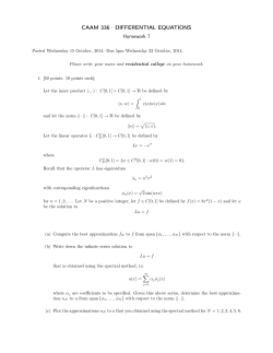
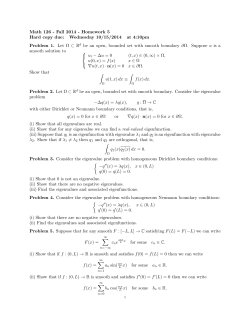


© Copyright 2026