ABC
docz
Explore
Log in
Create new account
Download
Report
No category
Untitled
������ - NELTS������������
DeerResistantGrassesFernsAnnuals
Scott County Fair Bluegrass Festival
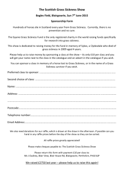
The Scottish Grass Sickness Show
3 2 1 Riley Blake
100 1 t S t = + 9 9 F t = +
The independent Turfgrass Experts for all your natural or synthetic
Gold Country Lions & Grocery Outlet`s 10th Annual Motorcycle Poker
Kenai`s changing fire regime
Cloudbridge Nature Reserve
© Copyright 2026
About abcdocz
DMCA / GDPR
Report