
Urban Travel Time Estimation from Sparse GPS Data
Urban Travel Time Estimation from Sparse GPS Data:
An Efficient and Scalable Approach
MAHMOOD RAHMANI
PhD Thesis
Stockholm, Sweden 2015
TRITA-TSC-PHD 15-005
ISBN 978-91-87353-72-7
KTH School of Architecture and Built Environment
SE-100 44 Stockholm
SWEDEN
© Mahmood Rahmani, June 2015
Tryck: Universitetsservice US AB, Stockholm 2015
iii
Rahmani, M., 2015. Urban Travel Time Estimation from Sparse GPS Data: An Efficient and
Scalable Approach. Department of Transport Science, KTH, Stockholm. ISBN 978-91-87353-72-7
Abstract
The use of GPS probes in traffic management is growing rapidly as the
required data collection infrastructure is increasingly in place, with significant
number of mobile sensors moving around covering expansive areas of the road
network. Many travelers carry with them at least one device with a built-in
GPS receiver. Furthermore, vehicles are becoming more and more location
aware. Vehicles in commercial fleets are now routinely equipped with GPS.
Travel time is important information for various actors of a transport
system, ranging from city planning, to day to day traffic management, to
individual travelers. They all make decisions based on average travel time or
variability of travel time among other factors.
AVI (Automatic Vehicle Identification) systems have been commonly used
for collecting point-to-point travel time data. Floating car data (FCD) timestamped locations of moving vehicles- have shown potential for travel
time estimation. Some advantages of FCD compared to stationary AVI systems are that they have no single point of failure and they have better network
coverage. Furthermore, the availability of opportunistic sensors, such as GPS,
makes the data collection infrastructure relatively convenient to deploy.
Currently, systems that collect FCD are designed to transmit data in a
limited form and relatively infrequently due to the cost of data transmission.
Thus, reported locations are far apart in time and space, for example with 2
minutes gaps. For sparse FCD to be useful for transport applications, it is
required that the corresponding probes be matched to the underlying digital
road network. Matching such data to the network is challenging.
This thesis makes the following contributions: (i) a map-matching and
path inference algorithm, (ii) a method for route travel time estimation, (iii)
a fixed point approach for joint path inference and travel time estimation,
and (iv) a method for fusion of FCD with data from automatic number plate
recognition. In all methods, scalability and overall computational efficiency
are considered among design requirements.
Throughout the thesis, the methods are used to process FCD from 1500
taxis in Stockholm City. Prior to this work, the data had been ignored because
of its low frequency and minimal information. The proposed methods proved
that the data can be processed and transformed into useful traffic information.
Finally, the thesis implements the main components of an experimental
ITS laboratory, called iMobility Lab. It is designed to explore GPS and other
emerging data sources for traffic monitoring and control. Processes are developed to be computationally efficient, scalable, and to support real time
applications with large data sets through a proposed distributed implementation.
Keywords: map-matching, path inference, sparse GPS probes, floating
car data, arterial, urban area, digital road network, iterative travel time estimation, fixed point problem, Stockholm, taxi.
Acknowledgements
I would like to express my special appreciation and thanks to my supervisor Haris
Koutsopoulos for his valuable guidance and support. I appreciate all his contributions of time, ideas, and funding to make my Ph.D. experience productive. I would
like to thank my assistant supervisor Erik Jenelius for his valuable inputs, support,
and collaboration. Special thanks to my wife Fayan for her personal support and
great patience at all times. I owe my deepest gratitude to my parents and friends
for their help and moral support.
I would also thank the following:
Traffic Stockholm: especially Tomas Julner and Jerk Brorsson; Info24: Hans Nottehed.
The Mobile Millennium Stockholm project team members at Sweco Infrastructure
AB, ITS & Traffic Analysis; Linköping University; UC Berkeley, Department of
Civil and Environmental Engineering, and California Center for Innovative Traffic
(CCIT); and KTH.
IBM Sweden: especially Erling Weibust and Niklas Dahl for their Hardware and
Software support.
My colleagues in the Swedish National ITS Postgraduate School.
My colleagues at KTH: senior researchers, administrators, fellow Ph.D. candidates,
and students.
Mahmood Rahmani
KTH Royal Institute of Technology
June 2015
v
Preface
The thesis includes the following five articles, for which I am the main contributor (from problem specification, research design, methodology development and
implementation to the analysis of results and writing):
I.
M. Rahmani, H. N. Koutsopoulos, and A. Ranganathan, “Requirements and
Potential of GPS-based Floating Car Data for Traffic Management: Stockholm Case Study”, 13th International IEEE Conference on Intelligent Transportation Systems, 2010, pp. 730-735.
II.
M. Rahmani and H. Koutsopoulos, “Path Inference from Sparse Floating
Car Data for Urban Networks”, Transportation Research Part C: Emerging
Technologies, vol. 30, pp. 41-54, 2013.
III.
M. Rahmani, E. Jenelius, and H. N. Koutsopoulos, “Non-Parametric Estimation of Route Travel Time Distributions from Low-Frequency Floating
Car Data”, Transportation Research Part C: Emerging Technologies, 2015,
in press, doi:10.1016/j.trc.2015.01.015.
IV.
M. Rahmani, H. N. Koutsopoulos, and E. Jenelius, “Travel Time Estimation
from Sparse Floating Car Data with Consistent Path Inference: A Fixed
Point Approach”, 2015, submitted.
V.
M. Rahmani, E. Jenelius, and H. N. Koutsopoulos, “Floating Car and Camera Data Fusion for Non-Parametric Route Travel Time Estimation”, 17th
International IEEE Conference on Intelligent Transportation Systems, 2014,
pp. 1286–1291.
Figure 1 illustrates a mapping between the five papers and various processing modules.
vii
viii
PREFACE
IV
IteraAve!Travel!Time!EsAmaAon!
!
!
FCD*!
database!
!
V !
!
ANPR**!
database!
!
I
II
Map2matching!!!
&!Path!Inference!
V
FCD!–!ANPR!!
Data!Fusion!
III
Travel!Time!
EsAmaAon!
III
!
EsAmated!
Travel!
Times!
I
Data!Management!and!Stream!Processing!Infrastructure!!
*!FCD:!floaAng!car!data!
**!ANPR:!automaAc!number!plate!recogniAon!
Figure 1: Illustration of the mapping between the 5 papers included in the thesis
and various processing modules.
I have contributed to the following papers (being the main author of one and
contributor of the rest):
VI.
M. Rahmani, E. Jenelius, and H. N. Koutsopoulos, “Route Travel Time Estimation Using Low-Frequency Floating Car Data”, 16th International IEEE
Annual Conference on Intelligent Transportation Systems, pp. 2292-2297,
2013.
VII. A. Biem, E. Bouillet, H. Feng, A. Ranganathan, A. Riabov, O. Verscheure,
H. Koutsopoulos, and M. Rahmani, “Real-Time Traffic Information Management using Stream Computing Need for Real-Time Traffic Information”,
Bulletin of the Technical Committee on Data Engineering, 2010.
VIII. A. Allström, J. Archer, A. M. Bayen, S. Blandin, J. Butler, D. Gundlegård,
H. Koutsopoulos, J. Lundgren, M. Rahmani, and O.-P. Tossavainen, “Mobile Millennium Stockholm”, 2nd International Conference on Models and
Technologies for Intelligent Transportation Systems, 2011.
IX.
E. Jenelius, M. Rahmani, and H. N. Koutsopoulos, “Travel Time Estimation
for Urban Road Networks Using Low Frequency GPS Probes”, Transportation Research Board TRB 91st, 2012.
X.
J. Ding, S. Gao, E. Jenelius, M. Rahmani, H. Huang, L. Ma, F. Pereira, and
M. Ben-Akiva, “Routing Policy Choice Set Generation in Stochastic TimeDependent Networks,” Transport Research Record, vol. 2466, pp. 76–86,
2014.
ix
XI.
J. Ding, S. Gao, E. Jenelius, M. Rahmani, F. Pereira, and M. Ben-akiva, A
Latent-Class Routing Policy Choice Model with Revealed Preference Data,
Transportation Research Board TRB, 2015.
Paper III is an extended version of VI. My contribution in paper VII is mostly in
its Section 2; estimating travel times of the Stockholm-Arlanda route. The paper
VIII is divided into arterial and highway sections. My contribution is the arterial
part and floating car data. In paper IX, I contributed to the the case study in
terms of data handling, network support and discussions. In papers X and XI, my
contribution is in their case study where I processed Stockholm taxi data using my
map-matching and path inference methods.
Contents
Acknowledgements
v
Preface
vii
Contents
xi
Part I, Introduction
1
1 Introduction
1.1 Background . . . . . . . . . . . . . . . . . . . . . . . . . . . . . . . .
1.2 Research gaps . . . . . . . . . . . . . . . . . . . . . . . . . . . . . . .
1
1
5
2 Research focus
2.1 Research questions . . . . . . . . . . . . . . . . . . . . . . . . . . . .
2.2 Limitations . . . . . . . . . . . . . . . . . . . . . . . . . . . . . . . .
7
7
8
3 Methodology
3.1 Map-matching and path inference . . . . . . . .
3.2 Route travel time distribution estimation . . .
3.3 Travel time estimation as a fixed point problem
3.4 FCD and ANPR data fusion . . . . . . . . . . .
.
.
.
.
.
.
.
.
.
.
.
.
.
.
.
.
.
.
.
.
.
.
.
.
.
.
.
.
.
.
.
.
.
.
.
.
.
.
.
.
.
.
.
.
.
.
.
.
11
11
12
13
14
4 Contributions
15
5 Conclusion and future work
19
Bibliography
23
Appendix
30
A The iMobility Lab
31
A-1 Introduction . . . . . . . . . . . . . . . . . . . . . . . . . . . . . . . . 31
xi
xii
CONTENTS
A-2
A-3
A-4
A-5
A-6
A-7
Data infrastructure . . . . . . . . . .
Computing infrastructure . . . . . .
Information infrastructure . . . . . .
Application and services . . . . . . .
Automated map error identification .
Software architecture . . . . . . . . .
Control flow . . . . . . . . . . . . . .
A-8 Network graphs and spatial indexing
Digital road networks . . . . . . . .
Spatial 2D indexing . . . . . . . . .
.
.
.
.
.
.
.
.
.
.
.
.
.
.
.
.
.
.
.
.
.
.
.
.
.
.
.
.
.
.
.
.
.
.
.
.
.
.
.
.
.
.
.
.
.
.
.
.
.
.
.
.
.
.
.
.
.
.
.
.
.
.
.
.
.
.
.
.
.
.
.
.
.
.
.
.
.
.
.
.
.
.
.
.
.
.
.
.
.
.
.
.
.
.
.
.
.
.
.
.
.
.
.
.
.
.
.
.
.
.
.
.
.
.
.
.
.
.
.
.
.
.
.
.
.
.
.
.
.
.
.
.
.
.
.
.
.
.
.
.
.
.
.
.
.
.
.
.
.
.
.
.
.
.
.
.
.
.
.
.
.
.
.
.
.
.
.
.
.
.
.
.
.
.
.
.
.
.
.
.
Part II, Papers
31
36
37
37
39
41
44
46
46
48
49
Paper I
51
Requirements and potential of GPS-based floating car data for traffic management: Stockholm case study . . . . . . . . . . . . . . . . . . . . . 51
I-1 Introduction . . . . . . . . . . . . . . . . . . . . . . . . . . . . . . . . 53
I-2 ITS laboratory for real-time traffic data processing . . . . . . . . . . 54
Data Infrastructure . . . . . . . . . . . . . . . . . . . . . . . . . . . . 54
Computing Infrastructure . . . . . . . . . . . . . . . . . . . . . . . . 54
Information Infrastructure . . . . . . . . . . . . . . . . . . . . . . . . 55
I-3 Stockholm taxi GPS data analysis . . . . . . . . . . . . . . . . . . . 56
Probe frequency . . . . . . . . . . . . . . . . . . . . . . . . . . . . . 56
Temporal coverage . . . . . . . . . . . . . . . . . . . . . . . . . . . . 56
Spatial coverage . . . . . . . . . . . . . . . . . . . . . . . . . . . . . 57
Analysis of travel time data . . . . . . . . . . . . . . . . . . . . . . . 57
I-4 Conclusion . . . . . . . . . . . . . . . . . . . . . . . . . . . . . . . . 58
Paper II
Path inference from sparse floating car
II-1 Introduction . . . . . . . . . . . .
II-2 Problem statement . . . . . . . .
II-3 Methodology . . . . . . . . . . .
Map-matching . . . . . . . . . .
Path inference . . . . . . . . . . .
Computational considerations . .
II-4 Application . . . . . . . . . . . .
Experimental design . . . . . . .
Evaluation . . . . . . . . . . . . .
Result . . . . . . . . . . . . . . .
II-5 Conclusion . . . . . . . . . . . .
II-6 References . . . . . . . . . . . . .
data
. . .
. . .
. . .
. . .
. . .
. . .
. . .
. . .
. . .
. . .
. . .
. . .
for urban networks
. . . . . . . . . . .
. . . . . . . . . . .
. . . . . . . . . . .
. . . . . . . . . . .
. . . . . . . . . . .
. . . . . . . . . . .
. . . . . . . . . . .
. . . . . . . . . . .
. . . . . . . . . . .
. . . . . . . . . . .
. . . . . . . . . . .
. . . . . . . . . . .
.
.
.
.
.
.
.
.
.
.
.
.
.
.
.
.
.
.
.
.
.
.
.
.
.
.
.
.
.
.
.
.
.
.
.
.
.
.
.
.
.
.
.
.
.
.
.
.
.
.
.
.
.
.
.
.
.
.
.
.
.
.
.
.
.
.
.
.
.
.
.
.
.
.
.
.
.
.
59
59
61
63
63
63
64
66
67
68
68
68
72
73
CONTENTS
Paper III
Non-parametric estimation of route travel time distributions
frequency floating car data . . . . . . . . . . . . . . . .
III-1 Introduction . . . . . . . . . . . . . . . . . . . . . . . .
III-2 Preliminaries . . . . . . . . . . . . . . . . . . . . . . . .
Network route travel time . . . . . . . . . . . . . . . . .
Travel time measurements from FCD . . . . . . . . . .
Sources of bias . . . . . . . . . . . . . . . . . . . . . . .
III-3 Methodology . . . . . . . . . . . . . . . . . . . . . . . .
Transformation . . . . . . . . . . . . . . . . . . . . . . .
Weighting . . . . . . . . . . . . . . . . . . . . . . . . . .
Aggregation . . . . . . . . . . . . . . . . . . . . . . . .
III-4 Application . . . . . . . . . . . . . . . . . . . . . . . . .
Data . . . . . . . . . . . . . . . . . . . . . . . . . . . .
Experimental design . . . . . . . . . . . . . . . . . . . .
III-5 Results . . . . . . . . . . . . . . . . . . . . . . . . . . .
Comparison with ANPR . . . . . . . . . . . . . . . . .
Analysis of FCD bias corrections . . . . . . . . . . . . .
Correction for non-representative vehicle sample . . . .
III-6 Computational performance . . . . . . . . . . . . . . .
III-7 Conclusion . . . . . . . . . . . . . . . . . . . . . . . . .
III-8 References . . . . . . . . . . . . . . . . . . . . . . . . .
xiii
from low. . . . . . .
. . . . . . .
. . . . . . .
. . . . . . .
. . . . . . .
. . . . . . .
. . . . . . .
. . . . . . .
. . . . . . .
. . . . . . .
. . . . . . .
. . . . . . .
. . . . . . .
. . . . . . .
. . . . . . .
. . . . . . .
. . . . . . .
. . . . . . .
. . . . . . .
. . . . . . .
75
75
77
78
78
79
79
80
80
82
84
84
84
85
86
86
89
91
93
95
95
Paper IV
Travel time estimation from sparse floating car data with consistent path
inference: A fixed point approach . . . . . . . . . . . . . . . . . . . .
IV-1 Introduction . . . . . . . . . . . . . . . . . . . . . . . . . . . . . . .
IV-2 Methodology . . . . . . . . . . . . . . . . . . . . . . . . . . . . . . .
Background . . . . . . . . . . . . . . . . . . . . . . . . . . . . . . .
Problem formulation . . . . . . . . . . . . . . . . . . . . . . . . . . .
Fixed point iteration . . . . . . . . . . . . . . . . . . . . . . . . . .
IV-3 Application . . . . . . . . . . . . . . . . . . . . . . . . . . . . . . . .
Data and algorithms . . . . . . . . . . . . . . . . . . . . . . . . . . .
Experimental design . . . . . . . . . . . . . . . . . . . . . . . . . . .
IV-4 Results . . . . . . . . . . . . . . . . . . . . . . . . . . . . . . . . . .
Convergence . . . . . . . . . . . . . . . . . . . . . . . . . . . . . . .
Impact on link travel times . . . . . . . . . . . . . . . . . . . . . . .
Impact on path travel time and shortest paths between OD pairs .
Sensitivity analysis . . . . . . . . . . . . . . . . . . . . . . . . . . .
IV-5 Conclusion . . . . . . . . . . . . . . . . . . . . . . . . . . . . . . . .
IV-6 References . . . . . . . . . . . . . . . . . . . . . . . . . . . . . . . .
97
97
99
102
102
103
104
107
107
108
109
109
112
114
114
118
119
Paper V
121
xiv
CONTENTS
Floating car and camera data fusion for non-parametric route travel time
estimation . . . . . . . . . . . . . . . . . . . . . . . . . . . . . . . . .
V-1 Introduction . . . . . . . . . . . . . . . . . . . . . . . . . . . . . . . .
V-2 Methodology . . . . . . . . . . . . . . . . . . . . . . . . . . . . . . .
Preliminaries . . . . . . . . . . . . . . . . . . . . . . . . . . . . . . .
Travel time estimation . . . . . . . . . . . . . . . . . . . . . . . . . .
V-3 Application . . . . . . . . . . . . . . . . . . . . . . . . . . . . . . . .
Experimental setup . . . . . . . . . . . . . . . . . . . . . . . . . . . .
Results . . . . . . . . . . . . . . . . . . . . . . . . . . . . . . . . . . .
V-4 Conclusion . . . . . . . . . . . . . . . . . . . . . . . . . . . . . . . .
V-5 References . . . . . . . . . . . . . . . . . . . . . . . . . . . . . . . . .
121
123
123
123
124
125
125
126
126
126
Chapter 1
Introduction
1.1
Background
Traffic congestion has become one of the major problems in large cities around the
world. With the continuous migration to cities the problem is growing (according
to the UN more than 50% of the world’s population now lives in cities). Cities
have been trying to alleviate congestion by increasing capacity, e.g. expanding
infrastructure, building high throughput roads, and supporting public transport.
On the demand side, city officials also try to recognize and change people’s travel
habits, and encourage travelers to use public transport alternatives. Other policies
include spreading peak hours and limiting traffic in certain areas by introducing
congestion pricing. Despite all these measures, the congestion problem is far from
solved.
In order to tackle traffic congestion problems, the transport system itself and
its interaction with the environment have to be better understood. Municipalities
have been trying to increase their knowledge about travel demand by collecting
data from different sources. In order to better understand travel patterns, i.e. how,
why, when, and from where to where people move, surveys are typically conducted
among citizens asking about their daily trips. This data collection method is usually
costly and is carried out infrequently, e.g. every several years. Such information
helps authorities to make strategic decisions.
Traffic control centers, on the other hand, need real-time data to estimate and
predict the state of traffic and make decisions on managing and controlling the
network. In this case, data is usually collected via stationary sensors such as loop
detectors, radar sensors, or cameras installed in the city. The cost of setting up and
maintaining traffic sensors is high. It is impractical to cover the entire road network
of a city by stationary sensors. Hence, many cities are looking for alternative or
complementary sources of travel and traffic data. In this regard, systems that are
built for other purposes but give the opportunity of collecting traffic information
are recently receiving a lot of attention.
1
2
CHAPTER 1. INTRODUCTION
Monitoring traffic conditions in light of increasing congestion in urban areas
is critical for traffic management and effective transport policy. One indicator of
traffic conditions is travel time which is used by network operators as an indicator
of quality of service. Provision of travel time information is also important as a
means of dealing with congestion. Examples of technologies for travel time data
collection include loop detectors and automatic vehicle identification (AVI) sensors
[11]. AVI systems, automatic number plate recognition (ANPR) cameras, and more
recently, Bluetooth devices provide direct measurements of travel times.
Devices with built-in GPS (Global Positioning System) receivers have become
popular. Many travelers carry with them at least one GPS-enabled device. Furthermore, vehicles are becoming more and more location aware. Dispatching systems
for taxis, delivery trucks, public transportation, ambulance services, etc. communicate, one way or another, with their counterparts moving around in the city and
collecting floating car data (FCD) which includes their timestamped geo-locations.
Such vehicles are also called probe vehicles. This type of opportunistic sensors are
already in place. Traffic authorities are interested in FCD because of: (a) no installation cost, (b) no maintenance expenses for third-parties, (c) extensive spatial
(and temporal) coverage, and (d) redundancy (if one sensor fails others can cover
for it).
Travel time can be estimated from FCD. But, since commonly available FCD
is sparse (less than once or twice per minute due to bandwidth limitations and
data transmission costs), vehicles may traverse multiple links between consecutive
probes, which means it is often challenging to estimate travel times from FCD [12].
FCD can be categorized based on penetration rate and frequency of reports.
Figure 1.1 illustrates the combinations of the two aspects. FCD that fall in the
lower-left category in this chart are difficult to use for traffic state estimation. The
number of vehicles is low, so the confidence in the data decreases. The lower-right
class provides rich and detailed data for very few vehicles. Although adequate
for capturing the dynamics at the link level, this type of FCD has low network
coverage. The upper-left category is the type of most of today’s available FCD,
mainly from fleet management systems. Thousands of vehicles in an urban area
report their location once in every 30 sec to 3 minutes. They usually have a small set
of attributes, geo-location, timestamp, and ID, and because the systems providing
such data use 10-20 years old technologies, they often do not have the ability to
add more attributes. Despite all processing difficulties associated with this group
of FCD, useful traffic information can be estimated with careful pre-processing.
Finally, the upper-right corner of the chart is the class of high-quality FCD. This
type of FCD is increasingly becoming popular but still not readily available. They
are rich with several attributes, e.g. speed, heading, and acceleration. Today, a
typical vehicle is equipped with several sensors and runs millions of lines of code.
Car manufacturers collect high resolution data from each vehicle for monitoring
and troubleshooting purposes. Such FCD, referred to as extended FCD, potentially
increase the accuracy of traffic state estimation. In addition, crowdsourcing FCD
becomes more and more common, where in addition to automatic location reports,
1.1. BACKGROUND
3
travelers may report what they experience, e.g traffic jams and accidents.
High penetration
•  Low quality
sparse
•  Uncertainty in path identification
•  Enough samples for aggregation
•  Most of today’s available FCD
•  Still useful
•  Less useful
•  Ideal
•  Promising to be more available
in future
frequent
•  Captures link/intersection
dynamics better
•  Not enough data for aggregation
•  Low spatial coverage
Low penetration
Figure 1.1: FCD Frequency versus penetration rate chart.
Today’s commonly available FCD are sparse with medium penetration rate.
Using such data has its own difficulties: (a) they are usually raw and need to
be preprocessed for traffic applications using advanced methods, (b) a digital road
network is required to map the geo-location data (latitude and longitude) to streets,
in contrast to the predefined locations of stationary sensors, (c) frequency of the
reports is low and that requires sophisticated pre-processing methods, (d) privacy of
individuals has to be preserved, and (e) the penetration rate of probe vehicles (the
ratio of the number of probe vehicles to the total number of vehicles in a region) is
usually low.
The challenge of matching geo-location data to digital road networks and path
finding can be explained better using a real example shown in Figure 1.2. In this
example, two locations are reported by a vehicle at times t0 and t1 . The first
location has four links in its vicinity and the second has two links. Eight paths
between the two points are feasible depending on which pair of links is selected
(much longer paths would be infeasible because the vehicle’s speed is limited). The
problems of matching the location points to a map and finding the most likely
path that connects them are known in the literature as the map-matching and path
inference problems respectively.
In addition to path inference, another challenge in the estimation of travel times
from FCD is the fact that probe vehicles do not report exactly at the beginning and
end of links/routes of interest. Therefore, their trajectories may partially overlap
4
CHAPTER 1. INTRODUCTION
with the link/route of interest.
t1,1
t1,2
t0
3
t0,1
4
1
2
t0,2
t1
2
t0,3
1
: GPS probe
: candidate matched point
: proximity search area
: link direction
: trajectory
t0,4
Figure 1.2: An example showing the challenge of finding path connecting two consecutive probes; 4 candidate links of one probe to 2 candidate links of the next
probe.
1.2. RESEARCH GAPS
1.2
5
Research gaps
The main gaps identified in the literature include:
Off/on-line path inference method for sparse FCD
The problem of map-matching has been addressed in the past mostly in the context
of navigation, assuming that frequent GPS probes are available [13]. More recently,
there has been a lot of interest in sparse FCD. Traffic authorities are interested in
utilizing FCD as means of collecting travel time data, and if possible, link flows
as well as origin-destination flows. Sparse FCD requires different approaches for
map-matching. A number of path inference methods for sparse FCD have been
proposed in the literature [14, 15, 16, 17], but they all rely on instantaneous speed
and heading in addition to geo-location and timestamp.
A method is needed for cases where minimum information (latitude, longitude,
and timestamp) is provided. Thus, it should be independent of attributes such as
heading, speed, and odometer that are used by existing methods.
While existing methods work on a complete set of probes from a trip, there is
a need to also be able to perform map-matching and path inference as the stream
of data arrives, meaning that the end of the trip data has not yet arrived.
Scalable real-time route travel time distribution estimation
Several studies have shown that link travel times can be estimated from FCD [18,
19, 20, 21]. Estimating different statistics of route travel time distributions based on
link travel times is not straightforward and there are few studies on the estimation of
route travel time distributions which are scalable. There is a need for a simple and
efficient method for estimating route travel time distribution that can be applied
to large networks in real-time.
Consistency between path inference and travel time estimation
Path inference for (sparse) FCD, in general, requires the knowledge of a priori link
travel times in order to infer paths that are temporally consistent with the observed
information. However, accurate link travel times may not always be available (indeed, they are the desired output of the estimation). Due to lack of good initial
travel times, the inferred paths of the vehicles are generally not consistent with
the estimated travel times. Given the assumption that travelers choose paths to
minimize some functions of travel time, it can be concluded that the path inference,
and hence travel time estimation, are biased. The mutual dependency of path inference and travel time estimation has only been addressed in a few previous studies
[22, 23].
6
CHAPTER 1. INTRODUCTION
Mobile and stationary traffic data fusion
Each data collection system has its own advantages and disadvantages. Stationary
sensors usually have less measurement noise than mobile sensors but their network
coverage is limited. On the other hand, mobile sensors, commonly installed in
fleet vehicles, cover relatively wider areas of the network but they suffer from low
penetration rate and low sampling frequency. Traffic state estimations can benefit
from fusion of data collected by various sources as they complement each other and
the fusion increases the robustness of the estimations. A recent study shows that
average travel times on a highway network can be estimated accurately and reliably
by fusion of FCD, loop detector data, and Bluetooth data [24]. There is a gap in
the literature when it comes to the fusion of stationary (e.g. ANPR) and FCD for
arterial networks [25].
Outline of the thesis
The thesis is organized as a collection of papers. It is divided into two parts: introduction and papers. The introduction part involves five chapters. Chapter 1
gives a background and overview of the problem. Chapter 2 enumerates research
questions. Chapter 3 describes the methodology. Chapter 4 summarizes the contributions. Chapter 5 concludes the thesis and illustrates future works. Part two
includes 5 chapter, one for each paper. Appendix A describes the development and
architecture of an ITS lab, called iMobility Lab, as one of the contributions of the
thesis.
Chapter 2
Research focus
This section describes the research focus presented in terms of research questions
and the limitations of the research.
2.1
Research questions
The purpose of the research is to develop methods to estimate the state of traffic in
an urban area, specifically travel time profiles using FCD. Moreover, the methods
are designed with the aim to be computationally efficient and scalable, so that they
can be applied on large-scale networks with millions of links and big data sets.
Another criterion considered in the development of the methods is the employment
of different levels of abstraction to provide flexibility in handling heterogeneous
data sources and meta data.
The thesis addresses the following research questions:
RQ1
What is the potential of using floating car/person data in transportation?
FCD are new data in transport systems. Some studies have shown the
potential of FCD in various applications, ranging from traffic state estimation to map correction, etc. At this early stage of development, there
is a need to further investigate the potential of FCD in transportation.
RQ2
What are the requirements for using floating car data in transportation?
FCD, similar to any other source of data, have their own limitations and
difficulties to work with. They require pre-processing, filtering, and a
computing infrastructure designed for processing large volumes of data.
More research has to be done to identify the requirements for utilizing
FCD in a transport system.
RQ3
How to make raw FCD suitable for transport applications?
Raw FCD are a sequence of timestamped locations and have to be translated into elements that are understandable for traffic and transport applications. Thus, the FCD collected by several vehicles have to be converted
7
8
CHAPTER 2. RESEARCH FOCUS
to flow, density, speed, travel time, etc per road, segment, region, and so
on. Methods have to be developed to perform such transformations.
Sparse FCD are sometimes considered to be not good enough for estimating traffic conditions in dense areas of a city, due to ambiguity in the
path taken by the vehicles. The question is whether or not such belief is
correct, and if large data sets of sparse FCD can be useful with the help
of advanced methods.
RQ4
What are the sources of bias when the probe vehicles do not represent the
entire population?
Generalizations of estimates from probe vehicles to the entire population
can be biased if the data are collected only by a particular group, e.g.
taxis. The reason is that such probe vehicles are not representative of the
whole population of vehicles in a city. The question is how to identify the
sources of bias and correct them.
RQ5
Is it feasible to develop methods that are computationally efficient for large
networks?
Advanced methods for estimating traffic conditions from sensory data
are usually computationally heavy. Applying such methods to the entire network of a city is often infeasible. The possibility of developing
computationally less demanding methods requires more research.
RQ6
What are the effects of initial assumptions about the traffic in a network
on the estimation of traffic state based on FCD?
When processing FCD for estimating travel times, some assumptions have
to be made regarding the state of the network. Specifically, many of the
proposed methods require an initial estimate of travel times. How does
the selection of the initial conditions affect the final estimates?
RQ7
How to fuse stationary and mobile travel time data? What are the gains?
Nowadays, every modern city is equipped with various traffic sensors.
The problem is that there is no single type of sensor that covers the entire network and meets all the requirements of traffic applications. Traffic
control centers are usually interested in a system that takes into account
all available data sources when answering traffic questions. The question is how to fuse different types of data and what the gains are from
combining them together.
2.2
Limitations
Although the methods developed in this thesis can also be applied on floating
person data, the focus of the research has been on floating car data. The underlying
assumption is that the reported locations belong to a vehicle. In the case of floating
person data, a pre-processing of the data is required to identify the transport mode.
2.2. LIMITATIONS
9
The map-matching and path inference methods introduced in this thesis are
designed for outdoor movements. This is a different concept compared to indoor
map-matching which is a popular topic in the field of mobile robots.
The thesis assumes a static definition of the digital road network. In reality,
road networks change over time, from simple changes in the direction of traffic for a
street to major changes in the infrastructure. Ideally, a digital road network should
be treated as a dynamic entity that changes over time and keeps track of changes.
The assumption of a static network is used in many studies and real applications
today and is not restrictive.
This thesis focuses on processing FCD after they are collected. How to plan and
collect data is an important topic but out of the scope of the thesis (for guidelines
see the handbook of travel time data collection [26]).
Chapter 3
Methodology
The thesis tackles the research questions listed in Chapter 2 by developing four
methods for:
• Map-matching and path inference,
• Route travel time distribution estimation,
• Travel time estimation as a fixed point problem, and
• Traffic data fusion.
Each method is discussed in detail in a corresponding paper. This chapter summarizes the methods and refers to the corresponding paper.
3.1
Map-matching and path inference
In order to find the most likely trajectory for a given sequence of FCD, a two-step
method is proposed: map-matching and path inference.
Map-matching
Map-matching identifies a set of links in the vicinity of each GPS probe and finds
a matched point along each link (for details, see Paper II, Section 3).
Path inference
Path inference finds the most likely path for a sequence of candidate map-matched
points and corresponding road network. Path inference consists of three steps:
• connecting candidate matched points with shortest paths
• building a candidate graph
11
12
CHAPTER 3. METHODOLOGY
• finding the most likely path in the candidate graph.
For details of the path inference method, refer to Paper II, Section 3.
3.2
Route travel time distribution estimation
The methodology for estimating the travel time distribution on a network route
using low-frequency FCD is a non-parametric kernel-based approach. The output of the estimation includes statistics of the travel time distribution of interest
(moments, percentiles, probability density function, etc.).
The estimation method consists of a sequence of steps: transformation, weighting, and aggregation. The first step transforms map-matched FCD observations
that only partially overlap with the network route to observations of the route
travel time. Each observation is then weighted according to its relevance as a route
travel time observation. The final step is to aggregate all weighted observations
and calculate the sought statistics.
Transformation
The first step of the methodology is to transform each FCD observation partially
covering the route into an observation of the actual route travel time. The step is
performed independently for each observation and consists of four processes: concatenation, allocation, scaling, and route entry time estimation (for details, see
Paper III, Section 3.1).
Concatenation. Depending on the length of the network route in relation to the
sampling frequency of the FCD, a vehicle may report multiple probes along the
route. It is reasonable, however, to consider one passage of a vehicle on the route
as one travel time observation. Consecutive observations from the same vehicle are
thus concatenated into a single travel time observation. The result is a new, smaller
set of FCD observations to be used in the subsequent steps of the methodology.
Allocation. The next step considers the FCD observations that partially traverse
the network adjacent to the route. For each observation, the observed travel time
is allocated between the network route and the adjacent network. The allocation
is based on the prior link travel times and the distance traversed on each link.
Scaling. While the allocation step estimates the time spent on the network route for
each FCD observation, the observations do not, in general, traverse the entire route.
The next step, therefore, is to scale up the travel time observations to the entire
route. Similar to the allocation, the scaling is based on the assumption that the
ratio between the travel time on the overlap route and the travel time on the entire
network route is the same as for the prior travel time estimates on the same sections.
3.3. TRAVEL TIME ESTIMATION AS A FIXED POINT PROBLEM
13
Route entry time extrapolation. The time that each probe vehicle passes the beginning of the network route (the route entry time) is in general not observed or may
not even exist if the vehicle joins the route at some point further along the route.
However, the route entry time is the basis for clustering observations and aggregating statistics. For each observation the route entry time, real or hypothetical,
is estimated based on the prior travel time estimates along the same lines as the
allocation and the scaling.
Weighting
After transformation, each route travel time observation is assigned a weight that
determines the influence of the observation in the estimation of route travel time
statistics. Observations are weighted for two reasons: to reflect the level of representativeness of the observation in relation to the route; and to correct for sampling
bias due to uneven coverage of the route (see Paper III, Section 3.2, for details).
Aggregation
The last step of the estimation process calculates statistics of the route travel time
distribution from the travel time observations and the associated weights. The
observations are aggregated based on the corresponding route entry time according
to pre-specified clusters (i.e. time-of-day intervals, weekday, season, etc.). For
details, see Paper III, Section 3.3.
In order to unbias for non-representative vehicle sample, a regression analysis
investigates the relation between route attributes and the deviation of FCD-based
travel times from those of the entire population observed by the ANPR system.
The estimated travel times are corrected by a model using significant explanatory
variables from the regression analysis (see Paper III, Sections 5.2 and 5.3).
3.3
Travel time estimation as a fixed point problem
Many map-matching and path inference methods make assumptions about initial
link travel times, especially in the application of the shortest path algorithm. However, true travel times are still not known, and the path inference results may thus
be inconsistent. This thesis addresses this problem based on a fixed point problem formulation. Let fD be a combined function of path inference and travel time
estimation and D a set of FCD. The fixed point xú = fD (xú ) of travel times can
be found as follows: initial travel time profiles x0 are used in the first iteration
to process D and estimate link travel time profiles, x1 = fD (x0 ). For the second
iteration, x1 is used as a priori profile to compute x2 , as x2 = fD (x1 ). The iterative
process continues until a termination criterion is met. Note that the same set of
FCD is used throughout the process. The estimates of one iteration (xk ) may be
smoothed (by an update rule e.g. the method of successive averages) before being
14
CHAPTER 3. METHODOLOGY
used in the next iteration. A summary of the process is given by the flowchart of
Figure 3.1. For details refer to Paper IV.
Initial travel times
FCD
Initialize
Do path inference
Do travel time estimation
Smoothed travel times
Estimated travel times
Do smoothing
No
Input/output
Process
Condition
Start state
Stop state
Termination
Criterion met?
Yes
Final travel times
Figure 3.1: The flowchart of travel time estimation as a fixed point problem.
3.4
FCD and ANPR data fusion
A method for fusion of FCD with data from ANPR system is introduced. ANPR
data are travel times collected from ordered pairs of cameras which identify vehicles
based on optical recognition of license numbers. An ANPR route is defined as the
path between the locations of the first and the second camera (more precisely,
the locations where vehicles are detected); it is assumed that there is a unique
reasonable route between the two locations. A data record is created whenever
the same vehicle is identified sequentially by both cameras. A record is a triplet
(h, s, e), where h is a unique ANPR route identifier, and s and e are the timestamps
of the detection of the vehicle at the first and the second camera, respectively.
The method first converts ANPR reports to timestamped trajectories (consistent
with the trajectory format of path inference output), then applies the route travel
time estimation method (introduced in Section 3.2) on a mixed data set of ANPR
and FCD trajectories. The method is described in detail in Paper V.
Chapter 4
Contributions
The contribution of each paper included in this thesis to the research questions
outlined in Chapter 2 are illustrated in Table 4.1.
Table 4.1: Relationship between research questions and papers.
Research question
RQ1
RQ2
RQ3
RQ4
RQ5
RQ6
RQ7
Papers
I-V
I, II
I-V
III
I-III
IV
V
RQ1: What is the potential of using floating car/person data in
transportation?
Authorities, although interested in utilizing FCD, tend to underestimate the usefulness of “sparse” FCD because they believe that the quality of the data is not
adequate. The thesis develops models, filters, and processes to turn raw sparse
FCD into traffic information (Paper I-III). It investigates how the data covers the
road network both spatially and temporally. It shows that reliable traffic information in terms of link/route travel times can be estimated from historical data
(collected over months or years) and is comparable to direct travel times observed
by dedicated stationary sensors. It demonstrates with a few scenarios (in Paper II)
the potential of using FCD to identify digital map issues and inconsistencies and
help fixing them. The research concludes that although sparse FCD are not ideal,
they can be used as an important resource for generating traffic information.
RQ2: What are the requirements for using floating car data in
transportation?
In paper I, the requirements of an ITS Lab are introduced. Although the focus
of the research is on FCD, this source of data is seen as one of many sources in
15
16
CHAPTER 4. CONTRIBUTIONS
the context of an ITS Lab; hence, a broader and holistic view of the problem is
considered in designing the infrastructure. In addition, the potential growth of the
number of sensors and their reporting frequency demands a scalable infrastructure.
An ITS center should be capable of processing extensive amount of traffic data, both
offline and on-line. During recent years, the stream processing paradigm -sometimes
referred to as map-reduce (because of one of its successful implementations)- has
attracted many big data applications. Paper I selects a stream processing platform,
IBM InfoSphere Streams, and demonstrates how a scalable FCD processing system
can be built.
RQ3: How to make raw FCD suitable for transport applications?
FCD provide a sequence of timestamped geo-locations. Without path inference,
the amount of information that can be extracted from such sequence of locations is
low. It only reveals how long it took the vehicle to drive from one geo-location to
the next. Therefore, raw FCD may answer questions like how long it takes to travel
between two arbitrary points on a network if and only if there have been reported
sequences containing the two selected points. With sparse FCD and relatively low
penetration rate, it is likely that no data matching such criteria can be found to
answer the question. Besides, raw FCD is incapable of answering questions like
what the travel time of a given path is. Map-matching and path inference are
important filters to turn x-y coordinates to a format that is understandable and
useful for traffic and transport applications, i.e. timestamped trajectories.
Several studies have shown that link travel times can be estimated from FCD
[18, 19, 20, 21]. In general, these methods allocate the travel time between two
consecutive probes to the traversed links. When it comes to routes, average route
travel times can be estimated from the average link travel times. However, a drawback of a link-based approach is that statistics of the route travel time distribution
(apart from the mean value) are not straightforward to derive from the travel time
distributions of the constituent links. For many applications, for example, monitoring of path travel time reliability, estimation of the variance and percentiles is as
important as the calculation of the mean. While several models have been proposed
[19, 27, 28, 8], they typically rely on strong assumptions about the functional form
of the link travel time distributions and the correlation structure. For real-time
applications, there is also a trade-off between the complexity of the model and the
computational efficiency of route travel time calculations.
Paper I, with the Stockholm-Arlanda example, shows how FCD (without mapmatching) can be used for estimating the travel time between origin-destinations
of a popular route. Paper II develops scalable map-matching and path inference
methods, which are used further to estimate travel times. Paper III introduces a
non-parametric travel time estimation method that is suitable for large scale networks. A key point of the method is that it is fast and can estimate the travel time
distribution of any arbitrary path (defined on the fly) using years of historical data
in a matter a second. The paper compares the estimated route travel times with
17
direct travel times from stationary sensors and that shows the method accurately
estimates the travel time distributions for several routes. It also discusses cases
where FCD-based estimates do not match the observed travel times due to some
biases, and how to correct them.
RQ4: What are the sources of bias when the probe vehicles do
not represent the entire population?
Estimation of traffic conditions based on FCD collected from professional fleets
(such as taxis) may be biased for several reasons. One example is the bias due to
differences in traffic rules applied to these fleets: e.g. taxis may be allowed to use
public transport infrastructure. Other biases may be due to differences in driving
behavior, or vehicle types. Paper III enumerates a number of sources of bias.
Among them is the fact that taxis are allowed to take bus lanes, which introduces
a bias to the estimated travel time of those links. The paper introduces a method
for correcting the bias with the help of other data sources.
RQ5: Is it feasible to develop methods that are computationally
efficient for large networks?
Computational efficiency is a requirement for today’s transport applications. Data
driven methods should be designed so that they can process large volumes of data for
a full size city network. The methods developed in this thesis -from path inference
to travel time estimation- are designed to be efficient and scalable. They have
been tested on large data sets (with 108 probes) and large-scale networks (with
105 links) and show good performance. Paper II, Section 4.3 illustrates that the
proposed path inference method can handle 50 probes per second (or 3000 probes
per minute). Thus, a single instance of the software can handle up to 3000 vehicles
reporting their location (on average) once per minute. The method scales up by
running multiple instances of the process. Paper III, Section 6, shows that the
route travel time estimation method can estimate the travel time distribution of a
path in a matter of a second and that it scales well for larger data sets.
RQ6: What are the effects of initial assumptions about the traffic
in a network on the estimation of traffic state based on FCD?
Paper IV tackles this question by proposing an iterative process for the joint path
inference and travel time estimation problem. The method converges to a fixed
point where the input and output link travel times are consistent. Results from the
Stockholm case study show that the method converges fast. The iterative method
increases the number of links that are included in the travel time estimation, compared to the standard approach (no iteration). In general, the iterative approach
makes initial and estimated travel times similar, which results in consistency between path inference and travel time estimation.
18
CHAPTER 4. CONTRIBUTIONS
RQ7: How to fuse stationary and mobile travel time data? What
are the gains?
AVI and FCD have complementary strengths as FCD provide network coverage
while AVI data provides more accurate measurements on specific route segments
(larger sample size). The combination of AVI data and FCD has not been studied
much in the literature [25]. A data fusion methodology for the estimation of freeway
space-time speed diagrams based on loop detector data, AVI and FCD has been
proposed [29]. A recent study proposes a travel time estimation method based
on fusion of FCD, loop detector, and Bluethooth data [24]. To the best of my
knowledge, no studies have combined ANPR and FCD to estimate travel time
distributions for arterial routes.
Timestamped FCD trajectories (the output of the path inference method) and
ANPR travel times are both measures of travel times from one point on a road
network to another along a trajectory. Such similarity makes it feasible to combine
the two data sets. Paper V proposes a data fusion method and illustrates in a case
study that the fusion increases the robustness of the estimation.
Other contributions
This thesis has also contributed to several projects:
• Establishing the iMobility Lab. The thesis contributed to the design and
implementation of an ITS Lab, named iMobility Lab1 . iMobility Lab was the
recipient of IBM’s Shared University Research Grant and IBM’s Smart Planet
award 2010. For details of the contribution, see Appendix A.
• Mobile Millennium Stockholm (MMS). The MMS project is funded by
the Swedish Transport Administration and is a collaboration between Trafik
Stockholm, UC Berkeley, KTH, Linköping University and Sweco. The aim
of the project is to assimilate the knowledge and experience gained from the
Mobile Millennium project at UC Berkeley and develop new methods for data
fusion [7]. The methods developed in this thesis have been integrated and are
running within MMS at Trafik Stockholm.
• Real-time stream computing. The path inference and travel time estimation methods are designed considering real-time stream processing requirements [30]. Hence, they can be used as operators in a graph of operators
within a stream processing framework. Each operator has a number of inputs
and outputs. The stream of input (GPS data) is processed by the path inference operator and a stream of results (timestamped trajectories) is sent out to
the travel time estimation operator. The processes can scale up horizontally
by adding more operators. For more detail see [6, 1].
1 www.imobilitylab.se
Chapter 5
Conclusion and future work
The increasing availability of floating car data and data from other emerging sensors facilitates a number of interesting applications related to traffic monitoring and
management. The thesis develops and implements the main components of an experimental ITS laboratory designed to provide the functionality needed to support
the use of such data. The laboratory takes advantage of different technologies such
as stream computing to provide the computational resources needed for real-time
processing of the large amounts of (potentially heterogeneous) data.
The thesis proposes a map-matching and path inference algorithm for sparse
GPS probes. The performance of the proposed method on data collected for a case
study in Stockholm indicates that the method is robust with respect to various
probing frequencies and performs favorably compared to methods recently proposed
in the literature. The method is used for both, off-line (for historical data) and online (for real-time data) applications.
The thesis also presents a non-parametric method for the estimation of the
distribution of travel times along routes from sparse FCD. The method provides
estimates not only of the mean but also any statistics of the route travel time
distribution. FCD has several sources of bias, including incomplete and uneven
coverage of the route, and partial coverage of the adjacent network. The method
involves a number of steps designed to reduce the impacts of these factors. It is
designed to be efficient for real-time, on-demand applications such as trip planning
services. Furthermore, many steps in the calculation procedure can be performed in
parallel which reduces computing time further. The thesis also discusses correction
of the bias due to non-representativeness of the FCD sample, when other data
sources, such as ANPR, are available.
An iterative (fixed point) process for a joint path inference and travel time
estimation problem is proposed. For evaluation purposes, a case study is used to
estimate travel times from taxi FCD in Stockholm, Sweden. The method converges
to a fixed point where the input and output link travel times are consistent.
Finally, the route travel time estimation method is used to fuse FCD and ANPR
19
20
CHAPTER 5. CONCLUSION AND FUTURE WORK
data. The approach combines the network coverage of FCD with the relatively more
accurate measurements on specific route segments of ANPR. Application results
suggest that the fusion increases the robustness of the estimation, meaning that
the fused estimate is always better than the worst of the two (FCD or ANPR), and
sometimes better than the best of them.
A number of future research directions have been identified. The proposed
path inference method infers the most likely path for a given sequence of probes.
The method can be developed further to capture the uncertainty in inferred paths
by generating multiple alternatives, with a measure of confidence provided for each
alternative. The confidence factor can be incorporated in the travel time estimation
method to put more weight on observations with higher confidence.
Travel time in an arterial network is composed of running time and stopped
delay time (due to e.g. intersection delays). The travel time estimation method
proposed in this thesis allocates observed travel times from FCD entirely to network
links without separating running times from delays. Mixing delays with running
times makes it difficult to estimate the time of crossing an intersection in different
directions (left or right turn and going straight). A future direction of research is
to distinguish running from delay times and estimate delays for left/right turns and
going straight.
Another direction for future research is to use digital road networks with histories of changes. Many studies assume a static definition of the digital road network
even though network changes take place all the time, ranging from simple changes
in speed limits to more serious ones, such as direction of traffic for a street or even
major infrastructure changes. There are several research questions in this regard:
What is the effect of using static road network? How can the network definition be
updated more frequently? Can FCD be used to detect that changes in the road network have taken place early? How to keep track of different versions of a network?
How to ensure that traffic data sets and network definitions are used consistently?
And finally, how to transfer the results of processing traffic data between different
versions of a road network (e.g. developing models to estimate statistics of network
links considering the changes of the underlying network over time)?
The proposed method of fusing FCD and ANPR requires further research to
evaluate the method on a varied set of network routes and data sources, and to
calibrate the parameters of the method to optimize the performance.
Data collection from different sources other than stationary traffic sensors is anticipated to grow in future. Wireless technologies enable vehicle-to-vehicle, vehicleto-infrastructure and infrastructure-to-vehicle communication. Utilizing such data
enriches the available information on traffic conditions and that accelerates needs
for data fusion for transport systems.
It is anticipated that in the future there will be higher penetration of mobile
phones and connected vehicles. The Internet of Things and high speed data transfer
networks will facilitate communication and interaction between consumers, products, and manufacturers. With improvements in battery life, the limitation on
the number of probes due to battery consumption will be relaxed, increasing the
21
number of reports per traveler. These trends will result in the collection of more
mobility data. More and better quality data will change systems and services in
cities, and consequently how people interact with their environment including their
travel behavior. Particularly, high resolution-high penetration floating car/person
data can improve existing methods (e.g. path inference, traffic estimation) and also
create new opportunities such as modeling the dynamics of traffic along network
links in greater detail and better understanding of the demand.
Bibliography
[1] M. Rahmani, H. Koutsopoulos, and A. Ranganathan, “Requirements and potential of GPS-based floating car data for traffic management: Stockholm case
study,” in 13th International IEEE Conference on Intelligent Transportation
Systems, pp. 730–735, IEEE, 2010.
[2] M. Rahmani and H. N. Koutsopoulos, “Path inference from sparse floating car
data for urban networks,” Transportation Research Part C: Emerging Technologies, vol. 30, pp. 41 – 54, 2013.
[3] M. Rahmani, E. Jenelius, and H. N. Koutsopoulos, “Non-parametric
estimation of route travel time distributions from low-frequency floating car data,” Transportation Research Part C: Emerging Technologies,
doi:10.1016/j.trc.2015.01.015, 2015.
[4] M. Rahmani, E. Jenelius, and H. N. Koutsopoulos, “Floating car and camera
data fusion for non-parametric route travel time estimation,” in 17th International IEEE Conference on Intelligent Transportation Systems, pp. 1286–1291,
2014.
[5] M. Rahmani, E. Jenelius, and H. N. Koutsopoulos, “Route travel time estimation using low-frequency floating car data,” in 16th International IEEE
Conference on Intelligent Transportation Systems, pp. 2292–2297, 2013.
[6] A. Biem, E. Bouillet, H. Feng, A. Ranganathan, A. Riabov, O. Verscheure,
H. Koutsopoulos, and M. Rahmani, “Real-time traffic information management using stream computing need for real-time traffic information,” Bulletin
of the Technical Committee on Data Engineering, 2010.
[7] A. Allström, J. Archer, A. M. Bayen, S. Blandin, J. Butler, D. Gundlegård,
H. Koutsopoulos, J. Lundgren, M. Rahmani, and O.-P. Tossavainen, “Mobile
Millennium Stockholm,” in 2nd International Conference on Models and Technologies for Intelligent Transportation Systems, 2011.
[8] E. Jenelius, M. Rahmani, and H. N. Koutsopoulos, “Travel time estimation for
urban road networks using low frequency GPS probes,” in TRB 91st Annual
Meeting Compendium of Papers, 2012.
23
24
BIBLIOGRAPHY
[9] J. Ding, S. Gao, E. Jenelius, M. Rahmani, H. Huang, L. Ma, F. Pereira,
and M. Ben-Akiva, “Routing policy choice set generation in stochastic timedependent networks,” Journal of the Transportation Research Board, vol. 2466,
pp. 76–86, 2014.
[10] J. Ding, S. Gao, E. Jenelius, M. Rahmani, F. Pereira, and M. Ben-akiva, “A
latent-class routing policy choice model with revealed preference data,” in TRB
94th Annual Meeting Compendium of Papers, 2015.
[11] C. Antoniou, R. Balakrishna, and H. N. Koutsopoulos, “A synthesis of emerging data collection technologies and their impact on traffic management applications,” European Transport Research Review, vol. 3, pp. 139–148, Oct.
2011.
[12] E. Jenelius and H. N. Koutsopoulos, “Probe vehicle data sampled by time
or space: consistent travel time allocation and estimation,” Transportation
Research Part B, vol. 71, pp. 120–137, 2015.
[13] M. A. Quddus, “High integrity map matching algorithms for advanced transport telematics applications,” PhD Thesis, Centre for Transport Studies, Imperial College London, UK, 2006.
[14] S. Brakatsoulas, D. Pfoser, R. Salas, and C. Wenk, “On map-matching vehicle
tracking data,” in Proceedings of the 31st international conference on very large
data bases, p. 864, VLDB Endowment, 2005.
[15] Y. Lou, C. Zhang, Y. Zheng, X. Xie, W. Wang, and Y. Huang, “Map-matching
for low-sampling-rate gps trajectories,” Proceedings of the 17th ACM SIGSPATIAL International Conference on Advances in Geographic Information Systems, pp. 352–361, 2009.
[16] Y. Zheng and M. Quddus, “Weight-based shortest path aided map-matching
algorithm for low frequency GPS data,” 90th Annual Meeting of the Transportation Research Board, 2011.
[17] T. Hunter, P. Abbeel, and A. M. Bayen, “The path inference filter: modelbased low-latency map matching of probe vehicle data,” in Algorithmic Foundation of Robotics X, pp. 591–607, Springer-Verlag Berlin Heidelberg, 2013.
[18] I. Sanaullah, M. Quddus, and M. Enoch, “Estimating link travel time from lowfrequency GPS data,” Transportation Research Board 92nd Annual, vol. 44,
2013.
[19] A. Hofleitner, R. Herring, P. Abbeel, and A. Bayen, “Learning the dynamics
of arterial traffic from probe data using a dynamic bayesian network,” IEEE
Transactions on Intelligent Transportation Systems, vol. 13, no. 4, pp. 1679–
1693, 2012.
BIBLIOGRAPHY
25
[20] F. Zheng and H. Van Zuylen, “Urban link travel time estimation based on
sparse probe vehicle data,” Transportation Research Part C: Emerging Technologies, vol. 31, pp. 145–157, 2013.
[21] B. Hellinga, P. Izadpanah, H. Takada, and L. Fu, “Decomposing travel times
measured by probe-based traffic monitoring systems to individual road links,”
Transportation Research Part C: Emerging Technologies, vol. 16, pp. 768–782,
2008.
[22] B. S. Westgate, “Vehicle travel time distribution estimation and map-matching
via Markov chain Monte Carlo methods,” PhD Thesis, Cornell University,
2013.
[23] X. Zhan, S. Hasan, S. V. Ukkusuri, and C. Kamga, “Urban link travel time
estimation using large-scale taxi data with partial information,” Transportation
Research Part C: Emerging Technologies, vol. 33, pp. 37–49, 2013.
[24] A. D. Patire, M. Wright, B. Prodhomme, and A. M. Bayen, “How much GPS
data do we need?,” Transportation Research Part C: Emerging Technologies,
in press, doi:10.1016/j.trc.2015.02.011, 2015.
[25] N.-E. E. Faouzi, H. Leung, and A. Kurian, “Data fusion in intelligent transportation systems: Progress and challenges – a survey,” Information Fusion,
vol. 12, no. 1, pp. 4 – 10, 2011. Special Issue on Intelligent Transportation
Systems.
[26] S. Turner, Travel time data collection handbook, vol. 34. Office of Highway Information Management, Federal Highway Administration, US Dept. of Transportation, Sept. 1998.
[27] B. S. Westgate, D. B. Woodard, D. S. Matteson, and S. G. Henderson, “Travel
time estimation for ambulances using Bayesian data augmentation,” The Annals of Applied Statistics, vol. 7, no. 2, pp. 1139–1161, 2013.
[28] M. Ramezani and N. Geroliminis, “On the estimation of arterial route travel
time distribution with Markov chains,” Transportation Research Part B,
vol. 46, pp. 1576–1590, 2012.
[29] J. W. C. van Lint and S. P. Hoogendoorn, “A robust and efficient method for
fusing heterogeneous data from traffic sensors on freeways,” Computer-Aided
Civil and Infrastructure Engineering, vol. 25, pp. 596–612, 2010.
[30] M. Stonebraker, U. Çetintemel, and S. Zdonik, “The 8 requirements of realtime stream processing,” SIGMOD Rec., vol. 34, no. 4, pp. 42–47, 2005.
[31] H. Bargera, “Evaluation of a cellular phone-based system for measurements
of traffic speeds and travel times: A case study from Israel,” Transportation
Research Part C: Emerging Technologies, vol. 15, no. 6, pp. 380–391, 2007.
26
BIBLIOGRAPHY
[32] S. Bekhor, M. Hirsh, S. Nimre, and I. Feldman, “Identifying spatial and temporal congestion characteristics using passive mobile phone data,” in Transportation Research Board 87th Annual Meeting, vol. 100, pp. 22–25, 2008.
[33] M. E. Ben-Akiva, S. Gao, Z. Wei, and Y. Wen, “A dynamic traffic assignment
model for highly congested urban networks,” Transportation Research Part C:
Emerging Technologies, vol. 24, pp. 62–82, 2012.
[34] V. Berinde, Iterative Approximation of Fixed Points. Springer, 2nd ed., 2007.
[35] D. Bernstein and A. Kornhauser, “An introduction to map matching for personal navigation assistants,” Princeton University, New Jersey Transportation
Information and Decision Engineering Center, 1996.
[36] A. Biem, E. Bouillet, H. Feng, A. Ranganathan, A. Riabov, O. Verscheure,
H. Koutsopoulos, and C. Moran, “IBM InfoSphere Streams for scalable, realtime, intelligent transportation services,” sigmod, 2010.
[37] M. Bierlaire and F. Crittin, “Solving noisy, large-scale fixed-point problems and
systems of nonlinear equations,” Transportation Science, vol. 40, no. Bottom
2000, pp. 44–63, 2006.
[38] L. Brouwer, “Über abbildung von mannigfaltigkeiten,” Mathematische Annalen, vol. 71, pp. 97–115, 1912.
[39] E. Cascetta and M. Postorino, “Fixed point approaches to the estimation of
O/D matrices using traffic counts on congested networks,” Transportation Science, vol. 35, pp. 134–147, 2001.
[40] E. Cipriani, S. Gori, and L. Mannini, “Traffic state estimation based on data fusion techniques,” in 15th International IEEE Conference on Intelligent Transportation Systems, pp. 1477–1482, 2012.
[41] C. Demir, B. Kerner, R. Herrtwich, S. Klenov, H. Rehborn, M. Aleksic,
T. Reigber, M. Schwab, and A. Haug, “FCD for urban areas: method and
analysis of practical realisations,” in the 10th World Congress and Exhibition
on Intelligent Transport Systems and Services (ITSS03), 2003.
[42] E. W. Dijkstra, “A note on two problems in connecion with graphs,” Numerische Mathematik, vol. 1, no. 1, pp. 269–271, 1959.
[43] F. Dion and H. Rakha, “Estimating dynamic roadway travel times using automatic vehicle identification data for low sampling rates,” Transportation Research Part B: Methodological, vol. 40, pp. 745–766, Nov. 2006.
[44] P. Furth, B. Hemily, T. Muller, and J. Strathman, “Uses of archived AVL-APC
data to improve transit performance and management: Review and potential,”
TCRP Web Document, vol. 23, no. June 2003, 2003.
BIBLIOGRAPHY
27
[45] B. Gedik, H. Andrade, K. Wu, P. Yu, and M. Doo, “SPADE: The System S
declarative stream processing engine,” in Proceedings of the 2008 ACM SIGMOD international conference on Management of data, pp. 1123–1134, ACM,
2008.
[46] P. Hart, N. Nilsson, and B. Raphael, “A formal basis for the heuristic determination of minimum cost paths,” IEEE Transactions on Systems Science and
Cybernetics, vol. 4, no. 2, pp. 100–107, 1968.
[47] R. Herring, A. Hofleitner, P. Abbeel, and A. Bayen, “Estimating arterial traffic
conditions using sparse probe data,” IEEE Conference on Intelligent Transportation Systems, Proceedings, ITSC, no. September, pp. 929–936, 2010.
[48] W. Huber, M. Lädke, and R. Ogger, “Extended floating-car data for the acquisition of traffic information,” in Proceedings of the 6th World Congress on
Intelligent Transport Systems, 1999.
[49] T. Hunter, R. Herring, P. Abbeel, and A. Bayen, “Path and travel time inference from GPS probe vehicle data,” Proceedings of the Neural Information
Processing Systems foundation (NIPS), Vancouver, Canada, 2009.
[50] E. Kazagli and H. Koutsopoulos, “Estimation of arterial travel time from automatic number plate recognition data,” Transportation Research Record: Journal of the Transportation Research Board, vol. 2391, pp. 22–31, Dec. 2013.
[51] G. Leduc, “Road traffic data: Collection methods and applications,” Institute
for Prospective Technological Studies, European Commission, 2008.
[52] K. Liu, T. Yamamoto, and T. Morikawa, “Feasibility of using taxi dispatch system as probes for collecting traffic information,” Journal of Intelligent Transportation Systems, vol. 13, no. 1, pp. 16–27, 2009.
[53] H. X. Liu and W. Ma, “A virtual vehicle probe model for time-dependent
travel time estimation on signalized arterials,” Transportation Research Part
C: Emerging Technologies, vol. 17, pp. 11–26, Feb. 2009.
[54] T. Miwa, T. Sakai, and T. Morikawa, “Route identification and travel time
prediction using probe-car data,” International Journal of ITS Research, vol. 2,
pp. 21–28, 2004.
[55] T. Miwa, D. Kiuchi, T. Yamamoto, and T. Morikawa, “Development of map
matching algorithm for low frequency probe data,” Transportation Research
Part C: Emerging Technologies, vol. 22, pp. 132–145, June 2012.
[56] M. F. Oshyani, M. Sundberg, and A. Karlström, “Consistently estimating link
speed using sparse GPS data with measured errors,” Procedia - Social and
Behavioral Sciences, vol. 111, pp. 829–838, Feb. 2014.
28
BIBLIOGRAPHY
[57] H. Robbins and S. Monro, “A stochastic approximation method,” The Annals
of Mathematical Statistics, vol. 22, no. 3, pp. 400–407, 1951.
[58] S. Sadeghianfar, MapViz : A framework for visualization of floating car data.
Master’s thesis, KTH Royal Institute of Technology, 2012.
[59] R. Schäfer and K. Thiessenhusen, “A traffic information system by means of
real-time floating-car data,” Proceedings of ITS World Congress 2002, Chicago,
USA, 2002.
[60] C. Scott, “Improved GPS positioning for motor vehicles through map matching,” in Proceedings of the 7th International Technical Meeting of the Satellite
Division of The Institute of Navigation (ION GPS 1994), pp. 1391–1400, 1994.
[61] Y. A. Shashkin, Fixed Points, Mathematical World (Book 2). American Mathematical Society, 1991.
[62] X.-w. She, Z.-c. He, P.-l. Nie, W.-l. Zeng, X.-k. Cen, and X.-b. Dai, “An on-line
map matching framework for floating car data with low sampling rate in urban
road network,” in Transport Research Board TRB 91st, 2012.
[63] D. Srinivasan, R. Cheu, and C. Tan, “Development of an improved ERP system
using GPS and AI techniques,” in Intelligent Transportation Systems, 2003.
Proceedings, vol. 1, pp. 554–559, IEEE, 2003.
[64] W. Thompson, “On the likelihood that one unknown probability exceeds another in view of the evidence of two samples,” Biometrika, vol. 25, no. 3,
pp. 285–294, 1933.
[65] M. Treiber and D. Helbing, “Reconstructing the spatio-temporal traffic dynamics from stationary detector data,” Cooper@tive Transport@tion Dyn@mics,
vol. 1, 2002.
[66] M. Treiber, A. Kesting, and R. E. Wilson, “Reconstructing the traffic state
by fusion of heterogeneous data,” Computer-Aided Civil and Infrastructure
Engineering, vol. 26, pp. 408–419, Aug. 2011.
[67] C. E. White, D. Bernstein, and A. L. Kornhauser, “Some map matching algorithms for personal navigation assistants,” Transportation Research Part C:
Emerging Technologies, vol. 8, pp. 91–108, Dec. 2000.
[68] Y. Meng, W. Chen, Z. Li, Y. Chen, and J. C. Chao, “A simplified mapmatching algorithm for in-vehicle navigation unit,” Journal of Geographic Information Sciences, vol. 8, 2002.
[69] J. Yuan, Y. Zheng, C. Zhang, X. Xie, and G.-Z. Sun, “An interactive-voting
based map matching algorithm,” Eleventh International Conference on Mobile
Data Management, pp. 43–52, 2010.
BIBLIOGRAPHY
29
[70] Y. Yuan, H. van Lint, F. van Wageningen-Kessels, and S. Hoogendoorn,
“Network-wide traffic state estimation using loop detector and floating car
data,” Journal of Intelligent Transportation Systems, vol. 18, pp. 41–50, 2014.
[71] W. Zeng and R. L. Church, “Finding shortest paths on real road networks:
the case for A*,” Journal of Geographical Information Science, vol. 23, no. 4,
pp. 531–543, 2009.
[72] M. Bernard, J. Hackney, and K. W. Axhausen, “Correlation of segment travel
speeds.” Proceedings of the 6th Swiss Transport Research Conference, 2006.
[73] M. Bierlaire, J. Chen, and J. Newman, “A probabilistic map matching method
for smartphone GPS data,” Transportation Research Part C: Emerging Technologies, vol. 26, pp. 78–98, 2013.
[74] T. Hastie, R. Tibshirani, and J. Friedman, The Elements of Statistical Learning. Springer, 2nd ed., 2009.
[75] T. Miwa, D. Kiuchi, T. Yamamoto, and T. Morikawa, “Development of map
matching algorithm for low frequency probe data,” Transportation Research
Part C: Emerging Technologies, vol. 22, pp. 132–145, 2012.
[76] B. W. Silverman, Density Estimation for Statistics and Data Analysis. Chapman & Hall/CRC Monographs on Statistics & Applied Probability, Taylor &
Francis, 1986.
[77] M. Tulic, D. Bauer, and W. Scherrer, “Link and route travel time prediction including the corresponding reliability in an urban network based on taxi floating
car data.” Transportation Research Board 93rd Annual Meeting Compendium
of Papers, 2014.
[78] J. W. C. van Lint and N. J. van der Zijpp, “Improving a travel-time estimation algorithm by using dual loop detectors,” Transportation Research Record,
vol. 2160, pp. 41–48, 2003.
[79] D. Work and A. Bayen, “Impacts of the mobile Internet on transportation cyberphysical systems: traffic monitoring using smartphones,” in National Workshop for Research on High-Confidence Transportation Cyber-Physical Systems:
Automotive, Aviation, and Rail, Washington, DC, pp. 18–20, 2008.
[80] P. J.-J. Herings, G. van der Laan, D. Talman, and Z. Yang, “A fixed point
theorem for discontinuous functions,” Operations Research Letters, vol. 36,
no. 1, pp. 89 – 93, 2008.
[81] E. Jenelius and H. N. Koutsopoulos, “Sampling by time or distance in probe
vehicle data: Implications for travel time estimation,” Proceedings of the Transportation Research Board Annual Meeting, Washington DC, 2012.
30
BIBLIOGRAPHY
[82] J. Eliasson, “A cost-benefit analysis of the Stockholm congestion charging system,” Transportation Research Part A: Policy and Practice, vol. 43, no. 4,
pp. 468–480, 2009.
[83] A. Steiner and A. Leonhardt, “A map generation algorithm using low frequency
vehicle position data,” in 90th Annual Meeting of the Transportation Research
Board, 2011.
[84] M. Fowler, Patterns of Enterprise Application Architecture. Addison-Wesley
Professional, 2002.
[85] R. A. Finkel and J. L. Bentley, “Quad trees a data structure for retrieval on
composite keys,” Acta Informatica, vol. 4, no. 1, pp. 1–9, 1974.
Appendix A
The iMobility Lab
A-1
Introduction
The methods developed in this thesis is a part of a bigger picture, which is the development of an intelligent transport system (ITS) laboratory. It aims at providing
the required infrastructure and information technologies for conducting research on
transportation problems. That involves traffic data collection, filtering and data
mining, organizing the data for future retrieval, simulations and modeling, and providing services for various types of users. This section introduces the ITS lab at
KTH, called iMobility Lab, and the contribution of this thesis in the development of
the Lab. Figure A.1 summarizes the lab and its interactions with the environment.
A-2
Data infrastructure
Data infrastructure refers to technologies that are already in place and used for data
collection. The lab takes advantage of the data, but installation and maintenance
of the data collection infrastructure is out of the scope of the lab. However, the
research in the lab can result into more effective data collection methods. As an
example, a study has shown the impact of sampling by time and distance on travel
time estimation of floating car data [81].
The lab works with various types of traffic and traffic-related data: floating car
data; counts and speeds from radar sensors; incident, accident, road work data;
travel time information from cameras; and weather data.
The main source of FCD is a fleet of more than 1500 taxis operating in the
Stockholm area. Each vehicle reports its GPS position, vehicle id, occupancy status
(hired or free) and timestamp at certain intervals.
31
32
APPENDIX A. THE IMOBILITY LAB
Data Infrastructure: Sensors and Information Technologies
Internet
Lab.
Computing Infrastructure:
Data Stream Handling, Databases
Information Infrastructure:
Models, Simulations, Algorithms
Decisions
Applications and Services
- traffic information
- demand management
- traffic prediction & management - multimodal trip planning
- fleet management
- Incident/emergency response
!
Figure A.1: The ITS lab’s infrastructures and applications
Flow and speed data collected by the Motorway Control System (MCS) in Stockholm is another source of traffic data. The MCS uses a number of microwave sensors
placed on a number of highway links in the network to collect the number of passing vehicles and the average speed per lane aggregated in 1-minute intervals. Thus,
every record consists of: detector id, timestamp, total flow, and mean speed in the
corresponding interval.
Another data source provides the road data which includes accident information,
road works, etc. it consists of timestamp, location, and estimated duration of the
event.
Automatic number plate recognition (ANPR) based on video processing is used
not only by the congestion pricing system, but also by the city to collect travel
time data on more than 100 selected routes. The system is deployed to support
the development of real-time travel time information for major arterials in the
Stockholm downtown area. A travel time observation is obtained from the difference
between the time stamps of a vehicle passing two cameras. Each travel time record
consists of a route id, a passage time, and time stamps for the detections by the
two cameras. Figure A.2 depicts the routes and location of cameras in Stockholm
inner city.
Stockholm introduced a congestion charging system with a tax that varies by time
of day. The system is based on number plate recognition through video technology.
!!
!(
!"
)#
)%
)*
#'
&$ &&
(*
!'
&!
&"
*'
""
%*
)!
"$
((%
)"
*"
*$
!&
%%
%#
!$
*)
&'
*&
%!
)(
"
(()
)'
)$
)&
%(
&(
!
#$
((*
#"
(!'
((#
$
%)
#)
*(
!)
%&
#&
&
)
!#
%$
%"
*!
(('
##
#%
(((
")
"&
0,0
0,5
"#
Kilometers
1,0
1,5
2,0
Rutter för mätningar av restider i
innerstaden 2009-2013
A-2. DATA INFRASTRUCTURE
33
Figure A.2: The routes and cameras for measurements of travel-times in the city
of Stockholm 2009-2013 (source: Swedish Traffic Road Administration).
34
APPENDIX A. THE IMOBILITY LAB
It provides data on flows by time of day. Figure A.3 shows the 18 detection stations,
strategically located at entry points to the inner city.
Figure A.3: The detection stations located at entry points to the inner city of
Stockholm (source: Eliasson et al. [82])
Buses are equipped with an automatic vehicle location (AVL) system that monitors the performance of the system and broadcasts related information (including
for example, how buses are running relative to the schedule).
Swedish Road Weather Information System (RWiS) consists of more than 700
weather stations located around the country, several in the Stockholm area (Figure
A.4). Each weather station measures wind speed and direction, air and road surface
temperature, air humidity and precipitation.
A-2. DATA INFRASTRUCTURE
35
Other traffic data, typical of legacy systems, are also available, such as counts and
speeds from loop detectors. The lab receives the FCD, MCS, ANPR, and incident
data in real-time.
N
Weather Station
Figure A.4: The map of weather stations in Stockholm (source: gis.vv.se/iov).
36
APPENDIX A. THE IMOBILITY LAB
A-3
Computing infrastructure
Integration and processing of the traffic data from diverse sources requires a computing platform that is scalable and flexible to support the diverse needs of the
various applications (ranging from real-time monitoring and control to archiving
and long-term planning), and facilitates development and implementation. The
computing platform should be able to handle data streams from all relevant sources
(motorways, urban streets, tunnels, transit, rail, weather, environmental sensors,
etc) and associated databases.
For the last 8 years clock speed of microprocessors has stopped advancing. Instead, CPU core count is increasing at the same rate as clock speed used to increase.
That means Moore’s law (the number of transistors on integrated circuits doubles
approximately every two years) is now achieved by increasing the number of cores.
Therefore, parallel and distributed computing is a way to take advantage of today’s
hardware and process huge volume of data. Parallel processing and concurrency
has always been a challenge for programmers because of non-determinism caused
by concurrent modules accessing shared objects.
On the other hand, applications that demand concurrent processing, particularly
on-line social networks, are now more and more common. That resulted in paying a
lot of attention to frameworks and languages that provide distributed and parallel
computing. Stream processing is a computing paradigm that has the potential
to satisfy the demand. The main requirements of (real-time) stream processing
include: keeping the data moving, having SQL capability on streams, handling
stream imperfections, predictable outcome, high availability, stored and streamed
data handling, distribution and scalability [30]. Hadoop1 and IBM InfoSphere2
are two examples of stream processing frameworks that have been examined in
iMobility Lab.
IBM’s stream processing framework, InfoSphere Streams, can filter, analyze, and
perform different tasks on streams of data in real-time. A case study at IBM Watson Lab developed a set of InfoSphere’s operators for GPS data [36]. It performs
different tasks such as data cleaning, matching to a map, etc. Figure A.5 shows
a data-flow graph that consists of a set of operators connected by streams. Each
operator implements data stream analytics. The operators communicate with each
other via their input and output ports. InfoSphere framework manages the execution of the graph of operators and can automatically scale up to multiple CPU
cores and scale out over a network of machines if it is needed.
1 http://hadoop.apache.org
2 http://www.ibm.com/software/data/infosphere/streams
A-4. INFORMATION INFRASTRUCTURE
37
In addition to frameworks, languages that support functional programing, e.g.
Scala, Ruby, etc., are also common in order to implement concurrent distributed
applications.
time-of-day,
day-of-week,
month-of-year
GPS
Source
f(x)
f(x)
KML
Color
map
5-min
aggr.
f(x)
Inter-quartiles
(IQ) weekends
ISO 8601 to Filter invalid
timestamp
values
GeoMatch
DSP
Clean Sort
f(x)
Adapt
IQ
f(x)
f(x)
f(x)
Travel
times
GPS Track
Sink
f(x)
IQ
f(x)
f(x)
Query Join
f(x)
Sink
f(x)
Current traffic
statistics
Figure A.5: A graph of operators representing a sample stream processing application used to analyze Stockholm taxi FCD.
A-4
Information infrastructure
The amount of traffic data collected over years can be huge. Hence, data management and organization are critical. The data is usually stored in databases with
proper indexing to facilitate record retrieval. Data cleaning is needed to detect and
remove duplications and outliers. The core traffic processes include: travel time estimation and prediction, traffic simulations, emission models, etc. Examples of the
traffic processes developed in the lab are path inference and two travel time estimation methods: a non-parametric high-throughput method [3], and a probabilistic
method [8]. Map-matching and path inference are two essential pre-processing units
in case of FCD processing.
A-5
Application and services
The vision for the Lab is to facilitate a number of applications spanning operations,
evaluation, and monitoring and control of transport systems. Examples include:
38
APPENDIX A. THE IMOBILITY LAB
Information generation and trip planning. The information can support a
number of applications at higher levels of precision than is currently available:
• door-to-door multi-modal trip planning
• traffic information for fleet management
Information about the reliability of the various alternative modes can also be included.
Testing and evaluation. Wide range of new technologies, systems, and concepts
can be tested and evaluated for traveler information services, advanced transportation and fleet management, inter-modal services/facilities from an operational point
of view, and demand management concepts (for example, new congestion pricing
strategies), etc.
Reporting and performance monitoring. The Lab, organized in the way
discussed here, can also help the monitoring of the system performance over time by
generating high level information appropriate for policy makers. For example, the
data collected can be used to estimate aggregate congestion performance measures
and help publish related reports for the region.
Travel time variability as a measure performance. Travel times and travel
time variability are important measures of quality related to the mobility of the
transport system in urban areas.
Archived data for planning and evaluation. The lab can serve as the repository of traffic and transportation related data, properly archived. Archived information is also useful to identify trends, changes in patterns, and point to problematic
areas, e.g. bottlenecks, etc.
Visualization Visualization has an important role in the Lab. Traffic data often includes geographical locations and it is always helpful to visualize such data
on a map and annotate streets based on some traffic attributes. In this regard, a
tool, called MapViz, was developed [58]. MapViz is a web-based framework that
facilitates visualization of geographical and traffic data through a flexible and extensible architecture. Extensibility is of major focus in this framework so that
various sources of data such as FCD, public transportation, etc can be fed to the
framework and be visualized on city maps. Figure A.6 shows a snapshot of the web
interface of MapViz.
A-6. AUTOMATED MAP ERROR IDENTIFICATION
39
Figure A.6: A snapshot of MapViz web UI. The dots represent taxis and the colorful
line segments are the trail of them while moving in the network.
A-6
Automated map error identification
FCD can be used to identify map errors (semi-) automatically and continuously.
Road networks are subject to change. Their geometry and traffic related attributes,
such as speed limit, direction of the traffic, maneuvering restrictions, etc. may
change over time. Digital road networks can have different errors or inconsistencies
compared to real road networks. iMobility Lab developed a method that detects
network errors automatically by processing sparse FCD (other methods, e.g. [83],
require frequent FCD). The example in Figure A.7 illustrates how the method
works. In this example, the path inference algorithm can successfully connect the
first probe to the second probe, but it cannot connect the second one to the third one
given network and travel time constraints. It fails because the digital road network
is inconsistent with the real road network. The street (denoted by dash line) is in
reality a two-way street but it is defined as a one-way street in the digital network.
In order to detect this kind of errors, one can run the path inference algorithm for a
large historical data against the city network and let the algorithm report frequent
problematic locations. Then one needs to check the reported locations manually
40
APPENDIX A. THE IMOBILITY LAB
1
2
Figure A.7: Map error detection using
FCD.
3
to determine the network errors. The path inference method can also report cases
in which probes are reported but in an empty space, i.e. the probes are off the
digital road network. An example of this case is shown in Figure A.8. The real
road network has changed in this picture because of the road construction. That
means vehicles are moving in temporary roads that are undefined in the digital
road map. Hence, the probes appear off the road. The path inference detects and
reports these cases.
Figure A.8: Norra Länken, Stockholm. The road network has changed because of
road constructions, but the changes are not reflected in the digital road network.
A-7. SOFTWARE ARCHITECTURE
A-7
41
Software architecture
The need for having a well-defined Software architecture originates from the fact
that software systems grow quickly as more and more modules are created over
time. Organizing and maintaining such big pool of modules after a while becomes
cumbersome. Multi-layer architectures are common practice [84]. In a layered architecture, components of each layer access the components in the next lower layer.
In technical terms, each layer has dependency to the layer below. The well-known
3-layer architecture consists of the data source, domain logic, and presentation logic
layers. The data source is the lowest layer and the presentation logic is the top-most
layer. The domain logic can itself be divided into multiple layers. For example, it
can involve core processes and on top of that a service layer (Figure A.9).
Domain Logic Layer
Presentation Logic
Layer
Service
Layer
Core Process
Layer
Visualization
Services
Feed
Readers
Log Files
Mobile
Apps
Travel-time
Services
Command Line
Interfaces
Journey Planner
Services
FCD
Travel-time
Estimator
Time-dependent
Travel-time
Profile
Path
Inference
Data Source
Layer
Rich
Clients
HTML-based
Clients
Map
Server
Journey
Planner
ANPR Data
Process
MCS Data
Process
Data Access Objsects (DAO)
Sensor
DB
Traffic
DB
GIS
DB
User
DB
Figure A.9: The 3-layer software architecture
The data source layer, also called persistent layer, is responsible for storing
and retrieving data to/from hard disks. This layer is equivalent to the computing
infrastructure block in the ITS Lab’s infrastructure diagram (Figure A.1). Database
management systems (DBMSs) and file systems are the most common components
of the data source layer. Storing data in files is more suitable for sequential processing purposes. DBMSs, on the other hand, provide fast search and random access
42
APPENDIX A. THE IMOBILITY LAB
to individual entries using indexing mechanisms and unique keys. Since traffic data
are usually associated with a geo-location, search and filtering based on location
is necessary. Many commercial and free DBMSs support geo-spatial indexing and
searching by providing GIS plug-ins. Indexing is a software mechanism that helps
retrieving data quickly without going through all records of data. Indexing is usually involves creating a tree, known as index tree. Section A-8 explains more detail
about geo-indexing.
This layer stores data from a wide range of categories. Sensory data in its raw
format (after basic filtering, e.g. removing duplications) are stored for further
processes. Intermediate results of the core processes are sometimes temporarily
stored on disks. The final output of the system is also stored to be used by end
users and services by request. Log files or log tables keep track of every step of
the processes and are useful for monitoring and debugging purposes. User profiles,
settings, access rights, etc. is also stored in the persistence layer. This layer includes
the following components:
• Sensor DB: tables that store different types of sensor data collected from
the city, including mobile sensors (FCD), stationary sensors (from radars,
cameras, and weather stations), and disruptions (incidents and road works).
• Traffic DB: tables that store the results of the traffic estimations and processes.
• GIS DB: stores the digital road network, maneuvering restrictions, etc.
• User DB: stores information about the users and their access right to various
parts of the system.
• Feed readers: are client programs that read data feeds from external sources,
for example from the traffic control systems or weather system.
• Log files: files that store different log files. Any component in different layers
may have logging requirements and the log files are centralized here.
• Data Access Objects (DAO): is a library of objects that are responsible for
read/write from/to the tables and files. These objects can be used by components in different layers to access the data. The only component that has
direct access to the database is DAO, the rest must access the data via methods provided by DAO.
The domain logic layer, also referred to as business logic, performs what the
software needs to do in the business domain, in this case traffic. It involves processing input and stored data, validation of the data, etc. Traffic simulation, travel
time estimation, path inference, traffic prediction, data filtering and mining, and
journey planning take place in the domain logic layer. The domain layer consists of
A-7. SOFTWARE ARCHITECTURE
43
core processes and services, that are equivalent to information infrastructure and
applications and services layer of the ITS Lab diagram (Figure A.1) respectively.
A brief description of the components in this layer is as follows:
• Map Server: loads digital road networks, handles indexing, finds geometrical
objects in the vicinity of another object, calculates distances between entities
on the map, and serves many other functionalities regarding the digital road
network. Any other component in this layer or the layers above that want to
use the road network has to work with the Map Server component.
• Path Inference: is responsible for map-matching and path inference of FCD
data. This component reads raw FCD from the Sensor DB or the Feed Readers, performs path inference and writes the results into the Traffic DB or any
other component that is registered as a listener of path inference results. In
observer design pattern [84] a subject (in this case the Path Inference component) notifies all its listeners (i.e. any other component that is interested in
path inference results, e.g. on-line travel time estimator) automatically.
• FCD Travel-time Estimator: estimates travel time of links by processing path
inference results. This component works in both off-line and on-line modes.
The off-line mode processes the historical data and the on-line mode processes
the stream of data from the Path Inference component. This component
contains different travel time estimation models (e.g. the non-parametric
model [3] and the arterial model [8]).
• ANPR Process: handles ANPR data cleaning, filtering, outliers detection,
and travel time estimation from ANPR data.
• MCS Process: handles MCS data cleaning, filtering, and travel time estimation from MCS data.
• (Time-dependent) Travel-time Profile: aggregates travel time information calculated from various types of sensors to answer questions such as travel time
from an origin to a destination at a certain time of day and day of week
taking into account traffic disruptions. This component reads the traffic information from the Traffic DB and the incident/roadworks from the Sensor
DB (all via DAO). Path Inference, FCD Travel-time Estimator, and Journey Planner modules work with Travel-time Profile module in order to access
time-dependent travel time of network links.
• Journey Planner: is the core component of journey planning. It finds the
shortest paths (in time or distance) between origin-destination pairs. The aim
of this component is to provide multi-modal journey planning. Journey Planner works with Travel-Time Profile to utilize time-dependent travel-times.
44
APPENDIX A. THE IMOBILITY LAB
• Visualization Services: provides services that can be used to visualize various
types of traffic information. In another words, it prepares the traffic information in a format that can be visualized. Components of the higher level have
to communicate with this module if they want to visualize the data in any
ways.
• Travel-time Services: is a facade object for all travel time related services (a
facade is a component that provides a simplified interface to a larger body
of the system [84]). Other modules and external clients call methods of this
service to retrieve travel time information. This component is the only entity
that invokes the core travel time modules directly.
• Journey Planner Services: is a facade object for journey planning. It works
directly with the core component of Journey Planner and with the Travel-time
services.
Any external clients (applications) or upper-level components has to work with
service modules as opposed to working with the core components directly.
The presentation logic layer is an interface for the services the system provides
to other systems, users, and client programs. This can be a command-line, a richclient graphics UI, a mobile app, or an HTML-based browser UI. The responsibilities
of this layer are to present information to the user and to translate user commands
to service invocations. The command line UI of map-matcher and the visualization
tool of Mapviz are concrete examples of the components that belong to this layer.
This software architecture layer fits in the applications and services layer of the ITS
Lab diagram (Figure A.1). The modules of this layer are as follows:
• Rich clients: are desktop programs that allows users to work with the different
services, from traffic information visualization to reports and demos.
• HTML-based Clients: provide access to the system via web. Mapviz is an
example of this type of clients that provides a user interface for the journey
planner, shows color-coded city maps with respect to travel time of links, and
demonstrates real-time FCD tracking [58].
• Mobile Apps: are applications that run on smart phones and work with the
lab’s services via Internet.
Control flow
Performing even a simple task in such a modular system requires a few components
interacting with each other. The components interaction is usually described using
a control flow diagrams. This section provides two examples of primary flow of data
and control in the iMobility Lab. The goal is to give an insight of how different
components interact with each other to realize some goals. The complete list of the
control flow is out of scope of this thesis.
A-7. SOFTWARE ARCHITECTURE
45
Feed readers interaction
Traffic data are usually collected by authorities, private companies, or crowd sourcing in a city. The raw data are typically dispatched to consumers using different
techniques. Pushing and polling are two common data transfer techniques. In the
pushing method, the data provider (or publisher) initiates the request for the transaction. In contrast, in the polling method the data consumer (or client) establishes
a connection to the data provider (called server in this case). Long polling is a
variation of the polling method that emulates the push method. A client requests
the server in a similar way to normal polling. The server holds the requests until
the data is available for response. Figure A.10 illustrates the interaction between
a feed reader and a data provider in the long polling method.
Data Source
(Server)
Feed Reader
(client)
DAO
Dispatcher
(data consumer)
initiate request
(TCP connection)
hold
transfer data
store data
hold
dispatch data
transfer data
store data
hold
dispatch data
...
transfer data
Figure A.10: Sequence of interactions between objects that realize data transmission
in a long polling method together with storing and dispatching.
Path inference interaction
The path inference task requires that a number of components work together. It
requires also a digital road network which is provided by the map server component.
It needs to know where to read the raw FCD data (source) and where to send the
results (sink). This requires working with data access objects (DAO) and consumers
of the path inference output. For example, a sink for the path inference results can
be a travel time estimator or a visual tracker. Figure A.11 depicts the interaction
of the components for the path inference.
46
APPENDIX A. THE IMOBILITY LAB
CLI
Map
Server
Controller
map-matching
command
create
network
Map
Matcher
DAO
load network
network data
new
create data source
Network
Graph
new
create data sink
Data
Source
new
Data
Sink
do map-matching
read
match
write
read
...
match
write
Figure A.11: Interaction between components in order to execute a path inference
command.
A-8
Network graphs and spatial indexing
Digital road networks
One of the essential components of a traffic lab that deals with real FCD is the
digital road network (DRN). Almost all traffic related processes (previously mentioned in the software architecture) require access to the underlying DRN. Hence,
this component should be carefully designed in order to avoid other components
suffering from its future changes. On the other hand, various formats of road networks are available; from commercial ones to free and open source ones. In order
to make the underlying DRN transparent from other components, adding a layer
of abstraction is necessary. Therefore, there will be an abstract DRN as a reference
and all components depend on it. A conversion mechanism is needed to read a
DRN and convert it to the abstract one. This also makes it possible to convert
from one DRN format to another using the abstract DRN as a mediator. Figure
A.12 illustrates the concept of abstract DRN. Network-dependent components only
depend on Network Graph, that means it is possible to switch between different
representations of the digital road network without affecting the dependent com-
A-8. NETWORK GRAPHS AND SPATIAL INDEXING
47
ponents. Each adapter knows how to load a network and convert it to the Network
Graph. The figure shows three sample adapters: NVDB (Swedish national digital
road network), OSM (Open Street Map) and Navteq.
Network Graph
A Network dependent
component
(e.g. map-matcher)
creates
Adapter 2
(OSM)
Adapter 3
(Navteq)
...
Network Factory
Adapter 1
(NVDB)
: dependency
: association
Adapter n
Figure A.12: The abstraction of the digital road network.
Network graph The graph representation of the road network contains information about the geometry and connectivity of the network. Edges represent streets,
and nodes represent intersections. The network graph is a directed graph, therefore, each bi-directional street is modeled by two links with opposite directions. A
link has a number of attributes such as:
1. unique ID
2. longitudes, a list of longitudes of the points defining the geometry of the link.
3. latitudes, a list of latitudes of the points defining the geometry of the link.
4. beginning node’s ID
5. end node’s ID
6. speed limit
7. next links’ IDs: determines the possibility of navigating from a link to its
succeeding links. The links in the next links’ IDs are those to which a vehicle
maneuver from this link.
8. opposite link’s ID: the ID of the link that provides the opposite direction of
this link.
9. function class: holds a value between 1 and 5 and represents the throughput
of the road. 1 is the highest throughput (e.g. highways) and 5 is the lowest
one (e.g. side streets).
48
APPENDIX A. THE IMOBILITY LAB
10. only bus/taxi lane flag: determines whether or not a link is a bus/taxi-only
lane.
11. traffic light: is a flag that is true if the link ends with a traffic light, and false
otherwise.
Merging and splitting links. One more consideration about the network is
dealing with long and short links. Digital road networks may contain links that
are a couple of kilometers long, and also links that are just one or two meters long.
Such extreme cases put unnecessary computation demand on the path inference
algorithm, and have side effects on travel time estimation as well [8]. Long links,
which occur on highways, can be split into shorter links, each a few hundred meters
long. Short links, on the other hand, can be merged to the neighboring links if the
geometry and network connectivity allows. That results in better path inference
performance (fewer number of candidate links) and better travel time estimation.
Spatial 2D indexing
Large-scale networks have thousands of links and finding neighboring links around
a particular point can be slow. Spatial indexing helps decrease the order of the
process by creating a hierarchy of regions so that eventually a small number of
comparisons is needed to find the area in the vicinity of a given point or object.
A number of indexing methods are developed for multi-dimensional spaces. Some
of them are considered optimum for node or link insertion and deletion. As the
network used in path inference remains static -no node or link is being added or
removed during run-time- a simple spatial indexing method called Quad tree or
Q-tree [85] is implemented.
Geo-spatial plugins Database management systems3 provide geo-spatial plugins that perform spatial indexing and search. The advantage of using these products
is that they are already implemented and tested by communities over years and
thoroughly tested. The disadvantage is that the map-matching program will have
to heavily use the database, and because database connections are normally slow especially when the database is running on a different machine than the one running
map-matching program- the database becomes the bottleneck of performance.
The software developed for this thesis takes advantage of PostgreSQL and its
spatial plugin, PostGIS4 . However, the map-matching software has its own built-in
indexing that makes it completely independent to the database.
3 For example: PostgreSQL (http://www.postgresql.org), MySQL (http://www.mysql.com),
Microsoft SQL Server (http://www.microsoft.com/sqlserver), and Oracle (http://www.oracle.
com/database)
4 http://postgis.refractions.net
A-8. NETWORK GRAPHS AND SPATIAL INDEXING
49
Figure A.13:
Leaves of a Qtree index for the
road network of
Stockholm city.
Darker cells refer
to more links.
Q-tree index A Q-tree index is defined as follows: each (usually rectangular)
region is divided into 4 subregions. Each subregion refers to the objects located in
it. If the subregion still contains large number of objects it is divided into 4 more
subregions. The parent region keeps pointers to its 4 children regions. This division
continues recursively until the subregions are small enough that hold a handful of
objects. The subregions in the lowest level are called leaves of the tree. Figure A.13
shows leaves of a Q-tree index for Stockholm city.
In order to search for links close to a probe, instead of computing the distance
between the point and thousands of links, one can first traverse the index tree from
the root node to find the leaf containing the probe location by a few comparisons.
Then all links in the leaf are examined by checking their perpendicular distance to
the point and the ones closer than a threshold are returned as the search results.
Cell borderline problem. Links close to the point of interest but in a different
cell than the point’s cell will be excluded in the search results. To overcome this
problem, as it is shown in Figure A.14, each cell refers to not only the links intersecting the cell’s box, but also the links located inside a slightly bigger surrounding
area. In another words, adjacent cells overlap in terms of the links they are referring
to.
50
APPENDIX A. THE IMOBILITY LAB
latitude
59.34
59.33
59.32
18.045
18.055
longitude
(a)
18.065
18.045
18.055
longitude
18.065
(b)
Figure A.14: 9 cells representing leaves of a Q-tree index (a), and the network links
to which the middle cell refers (b).


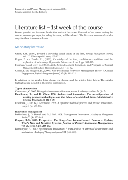


© Copyright 2026