ABC
docz
Explore
Log in
Create new account
Download
Report
No category
Splitting schemes for nonlinear parabolic problems
Math Analysis Honors – Worksheet 44 Multivariate Linear Systems
Lesson 5 Enrich Fractional Equations
Solving Systems of equations Video Lessons Directions: Watch all
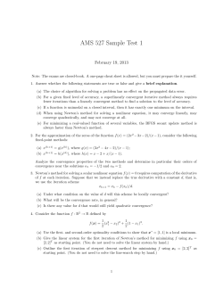
AMS 527 Sample Test 1 February 19, 2013
child care - WordPress.com
Cultural Divergence and Convergence
Math 1010 HW12 solutions p.294, #4. Use the ratio test.
ï global economy: a Europe-centered tale? ï the point of view
Fact Sheet: Income splitting vs Childcare
Homework 3 - METU | Department of Mechanical Engineering
© Copyright 2026
About abcdocz
DMCA / GDPR
Report