1. No category

SPE
6034
Optimal Design of Gas Transmission Networks
T. F. EDGAR
MEMBER WE-AIME
D. M. HIMLBLAU
T. C. BICKEL
ABSTRACT
This
study
presents
a computer
algorithm
to
optimize
the design o/ a gas transmission
network,
The technique
simultaneously
determines
(1) the
number of compressor
stations,
(2) the diameter
and length
of pipeline
segments,
and (3) the
operating conditions
o/ cacb compressor
station so
tba t the capital and operating costs are minimized, or
pro/it is maximized.
The literature has not reported
the
solution
o! such
an open-ended
problem,
altbougb
lesser
problems
have been solved
to
determine
the operating
conditions
of the gas
network
for a given configuration.
Two solution
techniques
were used.
One was the generalized
reduced gradi~nt method, a nonlinear programming
algorithm that could be used directly
in instances
where the capital costs of the compressors
were a
ftmction
of horsepower
output but had zero inita!
/ixed
cost.
Tbe second
method was applied
to
of
cases in which the capital costs are comprised
a rmnzero initial fixed cost plus some /un~tion of
horsepower
output. Here it was necessary
to use a
brancb=and.bound
scheme
with
the
nonlinear
programming technique mentioned above.
INTRODUCTION
The design or expansion
of a gas pipeline
system
involves
a large capital
transmission
expenditure as well as continuing operation and
maintenan cc costs. Substantial savings have been
reported (Flanigan,4
Graham et al.s) by improving
the system design for a given delivery rate. Both
the number and location of compressor stadons sad
the
operating
parameters
of each
must be
determined to obtain the minimum cost configuration.
%ich a Problem
involves
both integer
and
continuous variables because the optimal number
of compressor stations is unknown at the outset.
Receat developments
in nonlinear programming
(optimization) algorithms have made ava~lable new
techniques
for solving such a free configuration
Original manuscript received in Society of Petroleum Er@neore
office July 19, 1976. Pepar ●ccepted for publication June 14,
1977. Revised manuscript received Nov. 3, 1977. P*rmr (SPE
6034) was presented ●t the S l-t Annual Fall Technical Conference ●nd Exhibition, held irr New Orleans, Oct. 3-6, 1976.
0037-9999 /7S/0004-6034S00
.2S
Q 1978 Society of Petroleum Englneera
of AIME
1
U. OF TEXAS
AUSTIN, TEX.
design problem for a gas transmission
system.
This
paper describes
the gas pipeline,
its
“mathematical formulation
(a mixed-integer
programming p?oblem), the derivation of various cost
functions and constraints,
and two techniques for
solving the minimum-cost design problem. Two
example networks were solved. The first network
had gas entry at one point, with delivery to two
points. This problem was solved with and without
an initial fixed charge for the compressors.
The
second network was more general, consisting of a
multiple entry, mulriple delivery network. ft was
solved for the case of a zero fixed initial charge
for the compressor, The procedun
-.
.d aid in
the planning
and design
of ~~s pipelines,
acquisition of construction sites, and justification
of system modification.
THE PIPELINE
DESIGN PROBLEM
Suppose a gas pipeline is to be designed to
transport a skecified quantity of gas per time from
the gas wellheads to the gas demand points. The
initial states (pressure, temperature, and composition) of the gas at the wellheads and the fixed
states of the gas at the demand points are both
known. The following design variables need to be
determined (1) number of compressor stations; (2)
lengths of pipeline segments between compressor
stations, that is, station locations; (3) diameters
of the pipeline
segments;
and (4) suction and
discharge pressure at each compressor station.
Most published
investigations
of the above
problem have focused on design problems that fix
some of the above variables (subproblems of the
one posed above). One of the first investigations
of optimal operating
conditions
for a straight
(unbranched) natural gas pipeline with compressors
in series was performed by Larson and Wong.12
Their solution technique was dynamic programming,
and they found the optimal suction and discharge
pressures of a fixed number of compressor stations.
‘l%e length and diameter of the pipeline segments
were considered fixed because dynamic programming
was unable to accommodate a large number of
although it readily handled
decision
variables,
pressure
and compression
ratio cons”waints. A
comparison of their approach with the algorithm
tested in this paper is discussed later.
SOCIETY
OF ?CTROLEUM
ENGINEERS
JOUSNAL
,
.
.
Martch and McCall 1~ expanded the unbranched
pipeline configuration by adding branches to form
a network, and they posed the problem as one of
capacity
expansion
rather. than initial design.
Nevertheless,
the transmission network configura.
tion was predetermined
because the optimization
technique was dynamic programming and only the
pressures
were optimized.
Rothfarb
et al. 14
considered the csse where the network configuration
was not fixed. They investi,?ated
the optimal
selection of the pipeline diameters from a discrete
set of seven possible
sizes.
No compression
were optimized
in this investigation.
facilities
Heuristic procedures
for reducing the number of
possibilities
in the optimization
nlgorithrn were
introduced. Hence, this algorithm did optimize the
configuration,
requiring selection of both discrete
and continuous variables
(although all variables
were made discrete in this approach).
Programs offered by computer service” companies
to optimize gas pipeline
networks have been
described by Cheeseman2?s and Graham et al. Both
programs required postulation of the network, and a
large part of the software was oriented toward
solving
the
steady-state
flow md p~”essure
distribution for a single-phase gas network, although
Graham et al. added parallel branches to provide
greater capacity.
While complete details on the
mathematical
approaches
were not available,
it
appeared that the univariate
search method, in
which’ one variable was op’dmized at a time based
was used in both
on the partial
derivative,
algorithms. The univariate seaich method is not
considered a very powerful optimization method,
especially
for constrained optimization problems.
Compression
facilities
were added by trial and
error in these methods, and hence were not an
integrated part of the optimization procedure. One
heuristic feature of Cheeseman’s program was that
the compression ratios giving the minimum energy
consumption
should be equal for each station;
however, while this may be true for existing
compression
facilities,
it is not necessarily
investment
cost is
optimum when compressor
con sidered.
A more rigorous approach to the problem of
simultaneous optimization of compressor sizes and
pipeline diameters in a network has been presented
by Flanigan,
who used a constrained
steepestdescent method. Because the variables were not
independent,
Flanigan used linearized constraint
equations and required that the solution at each
step in the optimization
procedure represent
a
feasible point. This could increase the computing
time and required selection
of dependent
and
independent
variables,
necessitating
“judgment
and experience”
according
to Flanigan.
This
algorithm did not consider the optimization of the
number of compressors to be used in the network,
nor did it explicitly treat inequality constraints.
Anoiher constrained optimization procedure, based
on Kuhn-Tucker conditions, was proposed by Hax,g
who used it to determine
optimum operating
A?WL, 1971
conditions; this method was much more limited than
Flanigan’s”,
PROBLEM FORMULATION
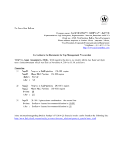
Fig. 1 illustrates
a simplified network used as
an example of the problem definition
and the
solution
technique.
The confimxation
of the
pipeline and the- characteristics
if the numbering
system for the compressor station and pipeline
segments are shown. Each compressor station is
represented by a node and each pipeline segment
by an arc between two nodes. Pressure increases
at a compressor station and decreases
along a
pipeline
segment.
The transmission
system is
horizontal. Although a simple example was selected
to illustrate the transmission system, a much more
complicated network can be accommodated, including
various branches and loops, at the expense of
increased computer solution time.
Fig. 1 shows these elements.
nc = total compressors;
?2=-1=
suction pressures
(the initial entering
pressure is known);
nc = discharge pressures;
= pipeline segment lengths (note
ns = *C +1
there are two segments issuing at the
branch point);
and
ns = n= + 1 = pipeline segment diameters.
Each pipeline st gment is associated
with five
variables: (1) the flow rate, q; (2) the inlet pressure,
P~ (tischarge
pressure from upstream compressor);
p= (suction
pressure of
(3) the outlet pressure,
downstream compressor); (4) the pipeline segment
diameter, d; and (5) the pipeline segment length, 2.
Where the mass flow rate through the pipeline is
predetermined, each compressor is assumed to lose
0.5 percent of the gas transmitted.
In this case,
only the last four variables
of each pipeline
segment need be determined.
The objective function of the pipeline is posed
)
..,,
“, ,“ “,
‘1
FaAxcn )
nwm
I
8
:,4
.,
●“,.*1
~
‘1 .“,
“,.
”,,.1
~“,+
1.
0
—
c-p,.,,,,,
,.(
.”,
1.
W.mcm 1
!,
.>
,.,
.,,
+.,
●
1
Plwllnr
5.,*.,
.,,
.
... .. ...”.
. .
.
“
‘1
“
‘1 ‘/
.
●I
‘!
,!
P
O.*
FIG. 1 _
PIPELINE
CONFIGURATION
WITH THREE
BRANCHES.
97
.
as a minimum cost problem. The objective function
is comprised of the yearly operating and maintenance
costs of the compressors
plus the sum of the
of the pipe
snd
costs
capital
discounted
compressors. Each compressor is assumed adiabatic,
with an inlet temperature equal co that of the
surroundings.
An efficiency
factor, q~, can be
used to correct for the mechanical efficiency of the
compressor (assumed to be 100 percent in this
study). One compressor’s
rate of work can be
described as
Line A, the objective
per year iS
P~
= 0.08531
p~
~)
-(
Ly-l
T s {1
z(Y-1/Y)
(1)
} 9***.*.**
s
where W‘ is expressed
in horsepower, y is the ratio
of the specific heats, the suction temperature, T~,
is expressed in ‘R, and z is the gas compressibility
factor.
Operating and maintenance charges per year, OY,
can be related directly to horsepower (Cheeseman)
and have been estimated at $8 to $14/hp-year
(Martch and McCall]. The annualized capital costs
for each pipeline segment, Cs, depend on the pipe
diameter and length, and have been estimated at
gS70/in.-mile-year (Marcch and McCall). Fig. 2 shows
two cost curves for tie capital expense
of the
cost is a linear
compressors.
Line A indicates
function of horsepower (Cc, the compressor capital
cost, is equal to $70/hp-year),
passing through
the origin. Line 8 also assumes a linear function
of horsepower (C. is equal to $69.50 /hp-year) with
a fixed initial capital outlay of $10,000, to account
for installation,
foundation, and other costs. For
cco = 10,000 Wr
HP-X - 20. WO hp
capital
slope
Co*t*
Cc
=
/
Z(y-1)
in dollars
/y
}+nfclljdj
{1-(+)
j=l
‘i
.
qJJ’
function expressed
. . . . . . . . . . . . . . . . .
,.
(2)
Although the objective function costs are linear
with respect to compressor output horsepower, the
ov?x-all objective function is nonlinear. Thus, any
continuous cost function with respect to horsepower
can be used for OY and Cc, and these cost functions
do not have to be linear to use the mathematical
technique.
For Line A of Fig. 2, where an initial fixed
the
charge does not exist for the compressors,
transmission network problem can be solved solely
by a nonlinear programming algorithm. on the other
hand, if the capital expense of the compressors
has an initial fixed charge (Line B of Fig. 2),
then the transmission
line problem becomes more
difficult and usually must be solved by a branchand-bound algori thin.
For Line A of Fig. 2, a branch-and-bound
technique
is not required because of the way
the objective
function
is formulated.
If the
~tio ~dt/pst = 1, the term involving Compressor r’
vanishes from the first summatioa in the objective
function, which is equivalent to deleting Compressor
i in a branch-and-bound
scheme. The pipeline
segments
joined at Node i may have different
If Line B represents
the compressor
diameters.
costs, the fixed incremental cost for each compressor in the system at zero horsepower (Cco) would
not be multiplied by the term in the square brackets
of Eq. 2. Instead, CCOwould be added, whether or
not Cbmpresaor i is in the system, if the nonliriear
programming technique was CObe used alone. Hence,
for Line B of Fig. 2, a different solution procedure,
one with nonlinear
namely, a branch-and-bound
programming, must be used, resulting
in much
longer computer times.
THE INEQUALITY
CONSTRAINTS
Each compressor is constrained so the discharge
pressure is greater than or equal to the suction
pressure,
P~
i
—>1
Ps
i
i=l,
. . . . . .
o
SOrqmrer
FIG.
2 — CAPITAL
AND OPERATING
COMPRESSORS.
..09nc*
2,
–
●
✎
✎
✎
✎
✎
✎
✎
✎
✎
✎
✎
✎
HPNX
COSTS
OF
and the compression ratio does not exceed
preapecified maximum limit K,
SOCIXTY
OF PETROLEUM
✎
(3)
some
ENGINECRS JOURNAL
TECHNIQIJES OF SOLUTION
A
in addition, upper and lower bounds at< placed on
each variable.
If the capital costs in the problem are described
by line A in Fig. 2, then the problem can be
by a nonlinea:
programming
solved
directly
algorithm. Of the many existing algorit~ms that
might he used,l” rhe generalized reduced gradient
nietbodl has beeu found to be generally superior
co other constrained multivar~akle methods.
The concept of the reduced gradient can be
illustrated
with a poblem of two variables [E
=(xl, @’l*
f(~)
Minimize
subject
and
(di)min
~ di
~
(di)maxo
. . . . . (5d)
to h(~)
=.
;
E
E2
()
. . .
Two classes
of equality constraints
exist for
the transmission
system. First, the length of the
system is fixed. There are two length constraints
for Fig, 1.
. s
The total derivatives of tic objective
the equality constraint are
●
●
●
●(9)
function and
&dx2. ..(lo)
df+dxl+jj
THE EQUALITY CONSTRAINTS
●
1
2
A
L
and
Observe that for feasible differential displacements
along the linearized
equality constraint,
Eq. 11
equals zero. Thus, one can solve for one displacement and eliminate the other from Eq. 10.
dq
.
.
,X2
[f--+]
●
●
‘(12)
and
where n
is’ the number of compressors
in Branch
i, net i~ the tot! .i number of compressors in the
first two branches,
and I ~ is the total length
between input and a given output. This type of
constraint does not reflect accurately the need to
select the optimal branch point. That would require
altering the distance constraints to account for the
of the supply-and-demand,
points.
A
geometry
simplified constraint form was used in this study;
the optimization
of the branch location will be
pursued later. The flow equation (the Weymouth
relation7 ) also must hold in each pipeline segment,
=
“
A dj813
‘;~
[1
- ‘:1
1’2
*
1’
. . . . . . . . . . . . . .
. . . . . . .(7)
where A = 8.71 x 10S and qj is the flow rate in
Segment j. To avoid problems in taking square
roots, Eq. 7 is squared to yield
~2d
16/3
‘
APSIL, 1971
(P:
-P:)
-ljq;
=o
””@)
dy
. . . ..o. (lq)
+~},
2
In this example, x ~ is eliminated as an independent
variable and the objective function is reduced to
an unconstrained
function of one independent
variable, X2, and one dependent variable, x 1 =
x1(x2). Once X2 is determined by the minimization,
xl is calculated from the difference equivalent of
Eq. 12 for small displacements.
Thus, a simple
unconstrained
minimization
along the direction,
d//dx2 (Eq. 13) yields a constrained minimum of
/(~). ~ Eq. 13, df/dx2 is known as the reduced
gradient because
it is expressed
in terms of
independent
variables
only.
This concept
is
equivalent to that used by Flanigan.
In vector notation for nv variables, of which mv
are dependent (subscript
D) and (n” - m~ are
independent
(subscript
f), and tnv independent
equality constraints
exist, the equations corre~
spending to Eqs. 10 through 13 are
j’
99
.
This linearization
with Newton’s method, rather
than a Hardy-Cross type method, is used to achieve
the flow and pressure distribution in the network.
●
O.*,.*
000..
..
.
(10a)
..**
BRANCH-AND-BOUND SOLUTION
TECHNIQUE
and
df(x)
=
k
.
.
.
d
.
.
.
.
..
.4
O.*
****
$
(13a)
Nonlinear equality constraints are transformed into
equality constraints
by squared slack variables,
except for the trivial bounds on the variables.
Let ~kl
be the value of the reduced gradient
vector evsluated
at some feasible
point E(h)
(defined by Eq. 13a). The generalized
reduced
gradient method be ins the search for the minimum
in the direction fio f defined as
Subsequent
search directions
are chosen by a
conjugate direction method such as the FletcherReeves recursion formulas that states
. . . . . .
●
✎
✎
✎
✎
✎
✎✎
☛☛☛✎
●
As explained,
with a fixed initial
capital
investment for the compressors
as indicated by
Line B in Fig. 2, a nonlinear programming algorithm
cannot
directly
solve
the transmission
line
problem. Instead,
a branch-and-bound
technique
combined with nonlinear programming must be used
to handle the integer variable.
A branch-and-bound
algorithm is nothing more
than an organized enumeration technique, used to
delete certain portions of the possible solution
set from consideration.
A tree is formed of nodes
and branches
(arcs).
Each branch i.n the tree
represents
a nonlinear
problem without integer
variables that is solved as explained above.
For exsmplej in Fig. 3, Node 1 in the tree
represents the original probiem as posed by Eqs.
2 through 8. When the problem at Node 1 is solved,
it provides a lower bad
ori the solution of the
problem posed by the cost function of Line B in
Fig. 2. Note that Line A always lies below Line
B. (If the problem at Node 1 has no feasible
solution, neither does the more complex problem.)
With the solution of the problem at Node 1, a
decision is made to partition on one of the three
integer variables, n= 1, nc ~~ or nc~ ~ which are the
number of compressors in Branches 1, 2, and 3,
respectively.
The partition variable is determined
when the smallest average compression ratio for
all the branches in the transmission
system
is
calculated
by adding all compression
ratios in
each branch and dividing
by the number of
compressors.
‘l%e number of compressors
in the
. (14)
It can be shown that these search directions are
constrained
to the hyperplanes
of, the locally
linearized active constraints.
In the presence of nonlinear constraints,
the
univariapt minimizations often lead to unfeasible E
A move into rhe unfeasible
region is
vectors.
limited by heuristic criteria. I Feasibility
is then
regained by using Newton’s method to solve the
F(ID) holding 11
set of nonlinear
equaticns
constant*
(a)
InitislProblem
CONSTBAXNTS:
Omclzk
0SC?53
omc3:3
(b)
F1 ret
where E~ designates
a point nearer the feasible
region. Iteration by Eq. 15 ia continued until the ‘
constraints reach the desired tolermce. The active
constraints then are relinesrized and a ncw reduced
gradient and search direction are calculated.
If
Eq. 15 does not converge, the variable basis is
altered
(selected
dependent
and independent
variables are interchanged) and Eq. 15 is reapplied.
190
FIG. 3-
BrmcnLns
PARTkAL TREE AND BRANCHES
EXAMPLE PROBLEM.
SOC3ZTY OF PXTROLUIM
FOR THE
ENGINEERS
JOURNAL
.
branch with the smallest
ratio becomes
the
partition
variable.
For example? in Fig. 3 the
partition variable was calculated to be nc2.
After choosing the partition variable, the next
step was to determine how the variable should be
partitioned.
Each compressor in the transmission
line branch associated
with the partition variable
was checked, and if any compressor operated at
less than 10-percent capacity, it was assumed to
be unnecessary
in the line. (If all operated at
greater than 10-percent capacity, the compressor
with the smallest compression ratio was deleted.)
For example, with n.cz selected, and onc of three
possible
compressors
at less than 10-percent
capacity, the first partition would lead to the tree
shown in Fig. 3b; n
would be either 3 or O s nc2
s 2. Thus, at each %ode in the tree the upper and
lower bound on the number of compressors in each
branch of the pipeline is readjusted.
The nonlinear problem at Node 2 will be the
same as at Node 1, with two exceptions. First, the
maximum number of compressors
permitted
in
Branch 2 of the ‘transmission
line is now two.
Second, the objective function is changed. From
the
lower bounds,
the minimum number of
compressors
in each branch of the pipeline is
known. For the lower bound, the costs related to
Line B in Fig. 2 apply; for compressors in addition
to the lower bound and up to the upper bound, the
costs are represented by Line A.
TABLE
SW ion
Pressure
Pe ,
P
P::
Pa4
P*5
P
so
P.7
F%a
Pe*
Pato
Dischtwge
Presewe
@
1 — COMPARISON WITH RESULTS
LARSON AND WOlW3
Lamon and
Wong
p$la)
QF
This Study
(psia)
Mm
620
!50ao
820
5s0
520
763,6
620
750
6S0
828.2
810
590
811.0
Ii?!?Q
J?s!2L
8CK)
605.7
5s8.7
526.1
5W.8
8W,0
Q53.1
Pda
t+j,
1,000
760
1,000.0
765.5
i@
840
641.8
pd6
950
951.5
Sa).o
Pde
1*000
Pda
1,000
pdto
770
1,000,0
1.000.0
787.3
Pout
5aJ
500.0
= 1.135242
A?SIL, 1~
X 10s
To test the effectiveness of the proposed solution
technique, an example problem formulated by Larson
and Wong was solved using as the objective
function the total horsepower of the compressors in
a long, straight pipeline.
In rheir problem, the
length and diameter of each pipeline segment were
fixed. Table 1 shows our results compared with
those of Larson and Wong, who used dynamic
programming.
Both the suction
and discharge
pressures differ from those of Larson and Wong in
many instances
because
their solution did not
satisfy the constraints
in their problem. Solving
the nonlinear
problem required
10 seconds of
755.1
1,000
Object
Ive function
NUMERICAL RESULTS
697.5
Pda
Pd,
As the decision tree descends, the solution at
each node becomes more constrained until ~odc z’
is reached, in which the upper and lower bounds
for the number of compressors
in each pipeline
branch are the same. The solution at Node i will
be feasible, but not necessarily
optimal, for the
general problem. Nevertheless,
the imptant
point
ie that the solution at Node i is an upper bound on
the solution of the general problem.
As the search continues through the rest of the
tree, if the value of the objective function at a
node is greater than that of the best feasible
solution found so far, then it is not necessary to
continue down that branch. The objective fimction
of any subsequent
solution found in that branch
would be larger than the solution already found.
Thus, we can fathom the node, that is, end the
search down that branch of the tree. The next ctep
is to backtrack up the tree and continue searching
through other branches until all nodes in the tree
have been fathomed. Another reason to fathom a
particular node is if no feasible solution exists to
the nonlinear
problem
at Node i; then all
subsequent
nodes below Node i also will be
unfeasible.
At the end of the search, the best soIution found
is the solution to the general problem.
objective function
= 1.1325189
X 10s
SYSTEM AND
FIG. 4 - INITIAL GAS TRANSM1SS1ON
FINAL OP’fIMAL SYSTEM USING THE COSTS OF LINE
A, FIG. 2.
m
.
pipeline
algorithm
‘6=--’”
FIG. 5-
OPTIMAL CONFIGURA~ON
USING THE
COSTS OF LINE B, FIG. 2.
central processing time on a CDC 6600 computer.
A more complicated network, using the initial
configuration shown in Fig. 4a and the cost relation
of Line A in Fig. 2, was then optimized. This
cost relationship
allowed direct application
of
nonlinear programming, but it did require the initial
postulation of compressor locations. The technique,
indicated
which compressor
when converged,
stations should be deleted. The maximum number
in Branches
1, 2, and 3 was
of compressors
specified
to be 4, 3, ~d 3, resFcUvelY.
Thc
entry pressure was 500 psia at a flow rate of 600
MMcf/D, and the two output pressures were set at
600 psia and 300 psia, respectively,
for Branches 2
and 3. The total length of Branches 1 and 2 was
constrained at 175 miles and of Branches I and 3
at 200 miles. While this geometry was unrealistic,
it
simplified
the pipeline
length
constraints
some what. The upper bound on the pipeline
diameter in Branch 1 was set at 36 in. and in
Branches 2 and 3 at 18 in., and the lower bound
on the diameters of all pipeline segments at 4 in.
These bounds were arbitrary and could be adjusted
after the results were obtained. A lower bound of
2 miles was placed on each pipeline segment to
assure
that the natural
gas was at ambient
conditions when it entered the next compressor in
the pipeline.
Fig. 5 compares the optimal gas transmission
network
with the original
network.
From an
unfeasible
starting
configuration Wia lo-mile
TABLE
VALUES OF OPERATING VARIABLES FOR THE OPTIMAL
CONFIGURATION
USING THE COSTS OF LINE A, FIG. 2
Pipeline
Sef3ment
Dlschsrge
Pressure
(@a)
SdOn
pressure
(psia)
Dimeter
(in.)
Length
(miie)
Flow
Rate
(hNcf/D)
1
2
3
4
5
6
7
8
9
10
11
119.1s6
1,000.OW
1,OW.fXJO
735.7S6
703.812
670.667
63S.133
735.766
5S5.262
89.126
832.457
715.399
6S9.352
735.786
703.812
670.657
636.133
6C0.t330
703.812
85S. 128
832.457
#XMIOO
35.0
32.4
32.4
18.0
18.0
16.0
18.0
18.0
16.0
18.0
18.0
2.0
51,3
113.7
2,0
2.0
2.0
2.0
2.0
2.0
2.0
27.0
5s7.0
5s4.0
591.0
m.o
292.6
2s1.1
26%7
294.0
‘2S2.6
291.1
2$0.7
TABLE
102
2 -
segments,
the nonlinear
optimization
reduced the objective function from the
first feasible state of $1.399 x 107/year to $7.289
x loVyear,
a savings of C1OSCto $7 million. of
compressor
stations,
only four
the 10 possible
remained in the final optimum network. Table 2
shows the final state of the network. The solution
of this problem required
353 seconds of central
processing time on a CDC 6600.
The nomenclature in Table 2 indicates that if
the suction pressure from the ith pipeline segment
was equal to the discharge pressure in the (i+ 1) th
segment, no compressor existed (and no cost was
added to the objective function, according to Eq.
2). Note that six compressors were removed. Also,
the constraints
on pipe length and diameter were
active in most pipes, indicating different constraint
values would give different converged results. Note
also that the optimal compression ratio was not the
same for all compressors for this problem because
of the effect of intervening pipe sections.
The problem described above and represented by
Fig. 1 was solved again using the costs represented
in Fig. 2 by Line B instead of Line A. Fig. 5 and
Table 3 present the results of the computations.
Note that Compressor
3 remained in the final
configuration
but with a compression ratio of 1,
indicating it was not performing. This means it was
cheaper to have two pipeline segments in Branch 1
and cwo compressors
operating at about one-half
capacity, pluc a penalty of $10,000, than to have
one pipeline segment and one compressor operating
at full capacity. Compressor 3 performing no work
represented
just a branch in the line plus a cost
penalty. About 900 seconds were required on the
CDC 6600 to obtain the optimal solution using the
branch-and-bound technique.
The final example solved is shown in Fig. 6a,
with tabulated
results
shown in Table 4. This
3 -
03mP;w
1
2
3
4
5
6“
7
s
9
10
VALUES OF OPERATiNG VARiABLES
FOR THE OPTiMAL
CONFIGURATION
USiNG THE C4XTS OF LINE B, FIG. 2
Pipeline
Disoharge
Prsaeure
&.Q!E!Q
1
2
3
4
5
-@!?l_&!?!ik
064.4S6
1,Oa).000
6SS.734
6SS.734
Q62.2W
Suotion
pressure
Dimmter
SS7.246
6s9.734
6W.~
666.6S4
m.am
J!!lJ-@!!l
32.3
32.3
15.2
18.0
16.9
Length
Flow
Rate
49.0
122.0
2.2
2.0
25.2
J!@!?EQ
5s7.0
594.0
295.!5
285.5
2s4.0
~a~n~r
1
2
3
4
NETWRK
COnwwr~oebn
1.44
1.40
1.12
1.00
1.00
1.00
1.00
1.2s
1.00
1.00
NE;-WRK
a~i~ion
1.91
1.19
1.W
1.43
EIWINEUS JO~NAL
SOCIXTY OF PCTROL8UM
TABLE
4-
VALUES OF OPERATING
VARIABLES FOR THE OPTIMAL
CONFIGURATION
USING COSTS OF LINE A, Fit%2
Cycscy
Suotlon
Pipeline
%Q!?!z&
1
2
3
4
s
6
7
8
Q
10
11
12
72Q.S
l,oa).o
S80.s
SS2.8
1,000.0
847.1
3s4.7
731.7
Sso.e
8s1.0
04?.1
610.4
Pfe8zure
Dkmwter
Length
=
-J!!!J_
28.63
31.76
20.1s
20.12
31.76
26.37
24.83
2C.63
24.34
24.27
14.22
14.01
@!!&
724.8
021.1
072.2
074.2
847.1
S41.S
6C0.O
724,6
073.s
074.2
610.s
300.0
multiple input-output ●xample was solved to show
how the technique can be applied to more general
networks. A bypass network also was added to
show the versatility
in describing
all possible
The bypass
segment
network
configurations.
of the original
problem
required
modification
structure because the flow through the bypass line
merged with the regular rtetwork.
described
a workable procedure for
transmission
line design that can be
treat much larger and more. complex
the ●xpense of considerable computer
NOMENCLATiiRE
A=
Cc =
Cl =
di =
E =
2.0
33.30
2.0
2.0
131.70
2.0
27.0
2,0
2.0
2.0
2.0
2.0
constant in Weymouth equation
annualized
capital
cost coefficient
for
compressor
annualized capital cost coefficient for pipe
diameter of jth pipe segment
Euclidean space
1
2
3
4
6
6
7
8
9
10
1.48
1.48
1.38
l.m
1.01
1.03
1.Q1
1.00
1.07
1,00
f = cost (objective;
gp
function
reduced gradidnt at kth iteration
equality constraint vector
upper bo~d on compression ratio
length of l’th pipe segment
total length of pipeline between supply and
demand points
total number of compressors in network
x
b=
Ki =
ii =
[,* =
in Branch i of
network
net = total number of compressors in a loop composed of two branches
total
number ?f pipeline segments
ns =
nv = total number of variables
% = total number of equality constraints
Oy = yearly operating cost coefficient
for
compressor
pd~= discharge pressure of ith compressor
Psi
9/
~(k)
=
suction pressure
=
volumetric
=
=
w’=
xi=
w-a
*,1,
z =
tWCtD
~s
Zm
CurQQdon
3W.O
6s4,0
237.7
238.6
6S6.0
201.0
220.0
18s.0
381.6
351.8
201.0
2s0.0
Ts
W
~~r
&!!k?Ql
nc =
n=, = total number of compressors
CONCLUSIONS
We have
optimal gas
extended to
net works, at
time.
Flow
Rate
NETWORK
=
=
;=
mc?ll
of ith compressor
flow rate in jth pipeline
search direction at kth iteration
programming
compressor suction temperature
compressor work
ith optimization variable
gas compressibility
factor
compressor efficiency
ratio of specific heats
gradient operator
segment
in nonlinear
WJBSCRIPTS
D = dependent
variable
1 = independent v&iable
500
27,
.)X7<
wt.
bw
,
mKrD
2.0
11.1
2.0
$
1.6
m
psi.
:.0
L Abadie,
$.
Generalia6,$>
L.
and (iuigop,
J.: “Gradient
Reduit
Note III 069/01, Electricity de France,
1S, 1969).
Clamant, France (Apil
7
2. Cheesemn,
ml mm
b]
LW711W-
WWICUMT1~
MITH
OP?!ML
?I?[LIN
[.ERGIIIS
(IR
Ill US)
FIG, 6 — INITIAL GAS TRANSMISSION SYSTEM AND
FINAL OPTIMAL SYSTEM USING l’HE COSTS OF LINE
A, FIG. 2.
APRIL, 1~
REFERENCES
2.
111.1
Q
z .0
2,0
~
1.0
8
A. P.:
“Full
Automation
DuxIgx process Appears Possible,”
(NOV.
of
Pipeline
Od usd Gas J.
15, 1971) Vol. 69, 147-151.
3. Cheeseman, A. p.: Wow to @timize
Design by Computer,”’ 011 d
GUS1.
Gas pipeline
(Dec. ’20t1971)
Vol. 69, 64-68.
m
4
●
.
4.
Flanlgsn, O.: f~conatra~ed Derivatives
Gaa Pipeline
System
optimization,”
j.
in Natural
Pet.
(May 1972) 549-556.
5. Fletcher, R. and Reeves, C, M.: “Function Minimization by Conjugate Directions,’: Computer J. (March
1964) Vol. 7, 149.
6. Garfinlcel,
R.
Pmgrammfwg,
S.
●nd Nernhauser,
G.
L.:
hrteger
John Wiley & Sons, Inc., New York
(1972).
7. Engineering Data Book, Gaa Processor
Assn., Tulua~ Okla. (1972).
Suppliers
8. Graham, G, E.,
Maxwell, D. A., and V8110ne, A.:
{tHow to optimize Ga8 Pipeline Networks?” PiPeii*e
hrd. (June 1971)41.43.
9. Hax, A, c.: ~~Naturai Gas Transmission syst~
Optimization: A Mathematical Programming Model,”
PhD dissertation, U. of California, Berkeley (1%7).
lU
10.Himmelblau, D. M.:
Applied Nonlinear Programming,
McGraw-Hill Book Co., Inc., New York (1972).
Tech
1L Katz, D. L.: Hadbook
o/ Nawal GUS Engineering,
.McGraw.Hill Book Co,, Inc., New York (19S9).
120 Larson, R. E. ●nd Won&
Natural Gss Systems via
IEEE
Tram. Asrlo. cOStt,
4759481.
13* Martch, H. B. and McCall,
the Design ●nd Operation
J.: ‘fOptimiza.ion
of
Dynamic Programming,~}
((%X,
196S) No. AC-12,
P.
●
N. J,: ‘~Optimization of
of Natural Gas Pipeline
Systems,”
paper SPE 4006 presented
at the SPEAIME 47th Annual Fall Meetin& San Antonio, Tex.,
oct. 8-11, 1972,
14. Rothfarb, B., Frank, H., Rosenbaum, D. M., Steiglitz.
K., and Kleitman, D. J.: “optimal Design of Off$horu
Res,
Natural Gas Pipeiine
Systems,~S Operations
(Nov.-Dee.
1970) 992-1020.
***