
Following the Trend: Tracking GDP when Long-Run Growth is Uncertain ∗ Juan Antolin-Diaz
Following the Trend: Tracking GDP when Long-Run Growth is Uncertain∗ Juan Antolin-Diaz Thomas Drechsel Ivan Petrella Fulcrum Asset Management LSE, CFM Birkbeck & CEPR This draft: November 20, 2014 First draft: October 24, 2014 Abstract Using a Bayesian dynamic factor model that allows for changes in both the long-run growth rate of output and the volatility of business cycles, we document a significant decline in long-run growth in the United States and in other advanced economies. Our evidence supports the view that this slowdown started prior to the Great Recession. When applied to real-time data, the proposed model is capable of detecting shifts in long-run growth in a timely and reliable manner. Furthermore, taking into account the variation in long-run growth improves the short-run forecasts and “nowcasts” of US GDP typically produced using this class of models. Keywords: Dynamic Factor Models; Bayesian Methods; Mixed Frequencies; Realtime Forecasting; Long-run growth; JEL Classification Numbers: C53, C38, C11, E37. ∗ Antolin-Diaz: Macroeconomic Research Department, Fulcrum Asset Management, Marble Arch House, 66 Seymour Street, London W1H 5BT, UK; E-Mail: [email protected]. Drechsel: Department of Economics and Centre for Macroeconomics, London School of Economics, Houghton Street, London, WC2A 2AE, UK; E-Mail: [email protected]. Petrella: Birkbeck, University of London, Malet Street, London WC1E 7HX, UK; E-Mail: [email protected]. The views expressed in this paper are solely the responsibility of the authors and should not be interpreted as reflecting the views of Fulcrum Asset Management. We thank Gavyn Davies, Wouter den Haan, Ed Hoyle, Ron Smith and the seminar participants at ECARES for useful comments and suggestions. Alberto D’Onofrio provided excellent research assistance. 1 1 Introduction “The global recovery has been disappointing ... Year after year we have had to explain from mid-year on why the global growth rate has been lower than predicted as little as two quarters back”. Stanley Fischer, August 2014. The slow pace of the recovery from the 2007-2009 recession has recently prompted questions about whether the long-run growth rate of the US economy (and other industrialised economies) is lower now than it has been on average over the past few decades. Indeed, for the last five years, forecasts of US and global real GDP growth have been persistently biased upwards. As means of illustration, Figure 1 shows the GDP growth projections made by the Federal Open Market Committee (FOMC) at the end of each year for the current year and the subsequent three. As the figure shows, actual GDP growth has averaged close to 2% over that period. At the end of each year, however, the FOMC expected the economy to accelerate substantially, only to downgrade the forecast back to 2% throughout the course of the year.1 What accounts for the systematic upward bias in growth forecasts? The present paper starts from the observation that there is substantial evidence of a decline in the mean of US real GDP growth. For instance, the structural break test of Bai and Perron (1998) suggests that a significant break in the mean GDP growth probably occurred in the early part of the 2000’s, and that this break is larger than the one generally accepted to have occurred in the early 1970’s (see also Luo and Startz, 2014). This evidence complements the recent work of Fernald (2014), who describes a slowdown in US labor and total factor productivity prior to the Great Recession, and concludes that most of the shortfall of actual output from the pre-recession trend is the result 1 The FOMC was not alone. An analysis of consensus forecasts of private sector economists, using data from Consensus Economics Inc., reveals the same pattern. 2 Figure 1: Year-end FOMC projections for US Real GDP Growth and Actual Outturn, 2009-2014 Actual Outturn Nov-09 Nov-10 Nov-11 Dec-12 Dec-13 6.0 4.0 2.0 0.0 -2.0 -4.0 -6.0 2009 2010 2011 2012 2013 2014 2015 2016 Note: Calculated as the midpoint of the central tendency of the FOMC participants’ individual projections. Both the projections and the actual outturn are expressed as percentage growth over the same quarter of the previous year. Source: Federal Reserve Board of Governors. of overly optimistic projections of potential growth. Interestingly, a sequential application of the Bai and Perron (1998) test using real-time data reveals that while the break is estimated to have occurred in the early 2000’s, it would not have been detected at conventional significance levels until the summer of 2014, which possibly explains the delay in incorporating the slowdown into growth forecasts. Orphanides (2003) emphasized that real-time misperceptions about the long-run growth of the economy can have a large role in monetary policy mistakes. We therefore argue that the possibility of significant instabilities in the mean (and the variance) of real output calls for a robust framework capable of producing timely assessments of short- and long-run GDP growth. To this end, we introduce two novel features into an otherwise standard 3 dynamic factor model (DFM) of real activity data: a time-varying long-run growth component for GDP, and stochastic volatility (SV) in the innovations to both factors and idiosyncratic components. While many econometric models have assumed long-run growth to be constant, and well approximated by the sample average of about 3%, the literature on economic growth reveals considerable uncertainty about the issue (see, e.g. Fernald and Jones, 2014). While it is by now widely accepted that the post-1973 sample is associated with a slowdown in productivity and therefore potential growth (see Nordhaus, 2004 for a retrospective), there is a range of views on the current prospects for the US economy after the booming years often associated with the IT revolution in the late 1990’s (Oliner and Sichel, 2000). In recent years a rather pessimistic view of long-run growth has emerged (Gordon, 2014, Summers, 2014) contrasting with more benign view of the health of the economy prevailing before the Financial Crisis (see Jorgenson et al., 2006). The introduction of a time-varying mean for GDP growth allows us to take the uncertainty about long-run growth seriously. As emphasised by Cogley (2005), if one thinks that the long-run growth rate is not constant, it is optimal to give more weight to recent data than to data from the distant past when estimating current longrun growth. By taking a Bayesian approach, we can combine our prior beliefs about the rate at which the past information should be discounted with the information contained in the data. The inclusion of SV is instead motivated by the desire to capture the changes in the uncertainty surrounding GDP forecasts in the sample under investigation. Specifically, this is important to capture the substantial changes in the volatility of output that have taken place during the postwar period, most famously the “Great Moderation” first reported by Kim and Nelson (1999a) and McConnell and Perez-Quiros (2000). Moreover, the recent literature on economic uncertainty finds substantial time variation and counter-cyclicality in aggregate uncertainty (see e.g., 4 Bloom, 2014, and Jurado et al., 2014). Since the seminal contributions of Evans (2005) and Giannone et al. (2006), the DFM has become one of the most important tools to produce real-time tracking estimates (also known as “nowcasts”) of GDP, for which data is available only quarterly and with considerable delay, by exploiting the ability of the Kalman Filter to incorporate the information content provided by more timely indicators.2 The DFM literature has generally operated under the assumption of no structural instabilities, either by assuming that the data is stationary to begin with, or that it has been differenced appropriately to reach stationarity.3 In the case of GDP, it is usually assumed that its quarterly growth rate has constant mean and variance. Important exceptions in the literature that allow for structural instabilities within the DFM include Del Negro and Otrok (2008), who model time variation in factor loadings and volatilities,4 and Marcellino et al. (2013), who show that the addition of SV improves the performance of the model for short-term forecasting of euro area GDP. Acknowledging the importance of allowing for time variation in the means of the variables, Stock and Watson (2012) pre-filter their dataset in order to remove any low-frequency trends from the resulting growth rates using a biweight local mean. In his comment to their paper, Chris Sims (2012) suggested to explicitly model, rather than filter out, these long-run trends, and emphasized the importance of evolving volatilities for describing and understanding macroeconomic data. We see the present paper as extending the DFM literature, and in particular its application to nowcasting GDP, in the direction suggested by Sims. 2 An extensive survey of the nowcasting literature is provided by Banbura et al. (2012), who also demonstrate, in a real-time context, the good out-of-sample performance of DFM nowcasts. 3 If evidence of structural breaks is present, the usual strategy is to select an estimation window over which the series are believed to be stationary. For example, Banbura et al. (2012) start their estimation sample in 1983 to account for the reduction in volatility associated with the “Great Moderation” in the mid-1980’s. 4 The model of Del Negro and Otrok (2008) also includes time-varying factor loadings, but the means of the observable variables are still treated as constant, i.e. they are stationary in the first moment but not in the second. 5 Because in-sample results obtained with revised data often underestimate the uncertainty faced by policymakers in real time, we conduct a careful out-of-sample evaluation of the performance of our model using vintages of US data from January 2000 to September 2014. We document how, by the summer of 2011 (well before the break test became conclusive) the model would have concluded that a significant decline in long-run growth was behind the slow recovery. Furthermore, we evaluate the forecasts of our model against a benchmark DFM without time-varying long-run growth or SV, and we show that the addition of these features improves both density and point forecasts of US GDP growth. Failing to account for the lower level of the long-run growth component of GDP, a standard DFM assuming a stable mean would have persistently predicted a recovery stronger than the one witnessed in the recent years. Finally, we apply our model to the other G7 economies and review the drivers of secular fluctuations of GDP growth. Our estimates conform to the well accepted narrative on the evolution of demographic and productivity trends in the advanced economies. We show that while in the US, long-run variations in productivity have been, until recently, masked by offsetting movements in labor force growth, in other countries productivity and labor force trends historically moved in the same direction, resulting in large changes in long-run output growth. We also show that productivity growth in the recent decade has been substantially below historical norms. Therefore, having a model that appropriately accounts for the uncertainty in the time variation of the long-run component of GDP is perhaps even more important at the current juncture. The remainder of this paper is organized as follows. Section 2 presents preliminary evidence of a slowdown in the long-run US GDP growth. Section 3 discussed the implications of time-varying long-run growth and volatility for DFMs and presents our model. Section 4 applies the model to US data and documents the decline in long-run 6 growth. The implications for tracking GDP are discussed in the context of our realtime out-of-sample evaluation exercise. 5 applies our model to the other G7 countries and decomposes the changes in long-run growth into its underlying drivers. Section 6 concludes. 2 Preliminary Evidence of a Decline in Long-Run GDP Growth The possibility that there are changes in long-run GDP growth is the source of a long-standing controversy, and has important implications for econometric modelling. In essence, the question is whether GDP growth is best described as fluctuating around a constant mean, or whether the mean growth rate is itself subject to stochastic variation. Nelson and Plosser (1982) first modelled the (log) level of real GDP as containing a random walk with drift. This implies that after first-differencing, the resulting growth rate would be stationary, and therefore exhibit a constant mean. Since their seminal contribution, this assumption has been embedded in many econometric models. After the slowdown in productivity and GDP growth of the 1970’s became apparent, many papers such as Clark (1987) modeled the drift term in the stochastic trend as an additional random walk. This second approach implies that the level of GDP is integrated of order two. This assumption would also be consistent with the local linear trend model of Harvey (1985), in the popular Hodrick-Prescott filter (Hodrick and Prescott, 1997), and in Stock and Watson (2012)’s practice of removing a local biweight mean from the growth rates before applying the standard DFM framework. The I(2) assumption is, however, not without controversy since it implies that the growth rate of output can drift without bound. Consequently, many applied papers, (see, e.g. Perron and Wada, 2009) have argued that the changes in trend growth 7 occurring in the 1970s reflect one large break, rather than a continuous sequence of very small breaks and modeled the growth rate of GDP as a stationary process with at most one deterministic break in the mean around 1973. As means of preliminary evidence of a slowdown in GDP growth, we test for multiple breaks in the mean of GDP growth over the postwar sample period using the Bai and Perron (1998) methodology.5 We find that there is evidence in favor of at least one break at the 5% level. The most likely break is in the second quarter of 2000, while the second most likely break, which is not significant, is estimated to have occurred in the second quarter of 1973. Figure 2: Real-Time Result of the Bai-Perron Test: 2000-2014 9 8 7 6 5 4 3 2000 2002 2004 2006 2008 2010 2012 2014 Note: The solid blue line is the test statistic obtained from recursively re-applying the Bai and Perron (1998) test in real time as new National Accounts vintages are being published. The dotted line plots 5% critical value of the test, while the dashed line plots the 10% critical value. These results are similar to those of Luo and Startz (2014), who use Bayesian model averaging to calculate the posterior probability of a single break and find the most likely break date in 2006:Q1. They note that if the sample was restricted to 5 See Appendix A for the full results of the test and some further discussions. 8 exclude the decade of the 2000’s, a break date around 1973:Q1 would be the most likely. This is also in line with the analysis of the labour productivity series by Fernald (2014), who finds evidence for three breaks in the mean growth rate of productivity: first, a productivity slowdown in 1973:Q2, second, a speedup around 1995:Q3, and finally a second slowdown in the early 2000’s.6 Given the somewhat different results obtained with different samples and methods, the precise number and timing of breaks remains unclear to us. However, it is a fair conclusion from the results presented above, that there is substantial evidence for at least one break in the mean of GDP in the postwar sample, most likely in the first half of the decade of the 2000’s. Most importantly, the early 2000’s break detected by the Bai and Perron (1998) test only became significant at standard levels with the recent vintages of National Accounts data, as displayed in Figure 2. If the test is correct and the break happened at the beginning of the decade, this means that the break was not detected until almost fifteen years later. This highlights the importance of an econometric framework capable of detecting changes in long-run growth in a timely and accurate manner. 3 Econometric Framework DFMs in the spirit of Geweke (1977), Stock and Watson (2002) and Forni et al. (2009) have become a workhorse of empirical macroeconomics. This popularity owes to their theoretical appeal (see e.g., Sargent and Sims, 1977 or Giannone et al., 2006), as well as their ability to parsimoniously model very large datasets. DFMs capture the idea that a small number of unobserved factors drives the comovement of a possibly 6 The results of Fernald (2014) vary slightly depending on whether the income or expenditure measures of GDP are used. In the first case, the breaks are detected in 1973:Q2, 1997:Q2 and 2003:Q1; in the second, 1973:Q2, 1995:Q3 and 2006:Q1. 9 large number of macroeconomic time series, each of which may be contaminated by measurement error or other sources of idiosyncratic variation. Giannone et al. (2008) and Banbura et al. (2012) have applied the DFM framework to the problem of nowcasting GDP; that is, obtaining early estimates of quarterly GDP growth by exploiting more timely monthly indicators and the factor structure of the data. The implications of the presence of instabilities in the mean of GDP growth for the estimation of DFMs are not straightforward. Intuitively, if the instabilities are shared by many of the series in the panel, they will be captured by the factors, and therefore the factor-based forecasts will be accurate. If, however, they are not common, they will be absorbed by the idiosyncratic component of GDP, while the factors themselves will still be estimated consistently (see Doz et al., 2012). Given the maintained assumption of stationarity of factors and idiosyncratic components, and given that the common factors drive most of the persistence in the series, the forecasts of the latter will revert to zero relatively quickly, likely producing biased forecasts and nowcasts of GDP. In addition, it is likely that the presence of instabilities in the variance will lead to poor density forecasting. In this section we propose to make the DFM framework robust to both of these instabilities. While, as noted by Luo and Startz (2014), the available data cannot conclusively settle the question of whether these instabilities take the form of discrete, large breaks, or a continuous sequence of small shocks, specifications with discrete breaks have very important practical drawbacks. First, until recently the presence of a single significant break in 1973 was usually taken for granted. This highlights the uncertainty about the number of true breaks and their exact timing. However, once a test is completed and a break introduced into a model, this is essentially asserting that the break(s) occurred with unit probability at the particular point determined by the test, therefore ignoring the uncertainty surrounding the test itself. Second, the fact that breaks have 10 occurred in the past should make the researcher wary that they might happen in the future. It follows that models with deterministic breaks underestimate the uncertainty around growth forecasts, which should increase with the forecast horizon. Finally, the real-time test result of Figure 2 made evident, structural break tests may only detect a break when it is too late. Therefore, while we remain agnostic about the ultimate form of structural change in the GDP process, we specify the long-run growth rate of GDP as a random walk. Our motivation is similar to Primiceri (2005). While in principle it is unrealistic to conceive that GDP growth could wander in an unbounded way, as long as the variance of the process is small and the drift is considered to be operating for a finite period of time, the assumption is innocuous. Moreover, modeling the trend as a random walk is more robust to misspecification when the actual process is indeed characterized by discrete breaks, whereas structural break tests might not be robust to the true process being a random walk.7 Finally, the random walk assumption also has the desirable feature that, unlike stationary in models, confidence bands around GDP forecasts increase with the forecast horizon, reflecting uncertainty about the possibility of future breaks or drifts in trend growth. 3.1 The Model Let yt be an (n × 1) vector of observable macroeconomic time series, and let ft denote a (k × 1) vector of latent common factors. It is assumed that n >> k, so that the number of observables is much larger than the number of factors. Setting k = 1 7 We demonstrate this point with the use of Monte Carlo simulations, showing that a random walk trend ‘learns’ quickly about a large break once it has occurred. On the other hand, the random walk does not detect a drift when there is not one, despite the presence of a large cyclical component. See Appendix B for the full results of these simulations. 11 and ordering GDP growth first (therefore GDP growth is referred to as y1,t ) we have8 y1,t = α1,t + ft + u1,t , yi,t = αi + λi ft + ui,t , (1) i = 2, . . . , n (2) where ui,t is an idiosyncratic component specific to the ith series and λi is its loading to the common factor.9 Since the intercept α1,t is time-dependent in equation (1), we allow the mean growth rate of GDP to vary. We choose to do so only for GDP, the variable of primary interest, to keep the model as parsimonious as possible.10 If some other variable in the panel was at the center of the analysis or there was suspicion of changes in its mean, an extension to include additional time-varying intercepts would be straightforward. In fact, for theoretical reasons it might be desirable to impose that the drift in long-run GDP growth is shared by other series such as consumption, a possibility that we consider in the robustness section. The laws of motion for the factor and idiosyncratic components are, respectively, Φ(L)ft = εt , (3) ρi (L)ui,t = ηi,t (4) 8 In our application to US real activity data, the use of one factor is appropriate and thus focus on the case of k = 1 for expositional clarity in this section. 9 The loading for GDP is normalised to unity. This serves as an identifiying restriction in our estimation algorithm. Bai and Wang (2012) discuss minimal identifying assumptions for DFMs. 10 The alternative approach of including a time-varying intercept for all indicators (see, e.g. Creal et al., 2010 or Fleischman and Roberts, 2011) implies that the number of state variables increases with the number of observables. This not only imposes an increasing computational burden, but in our view compromises the parsimonious structure of the DFM framework, in which the number of degrees of freedom does not decrease as more variables are added. It is also possible that allowing for time-variation in a large number of coefficients would improve in-sample fit at the cost of a loss of efficiency in out-of-sample forecasting. For the same reason we do not allow for time-variation in the autoregressive dynamics of factors and idiosyncratic components, given the limited evidence on changes in the duration of business cycles (see e.g. Ahmed et al., 2004). 12 Φ(L) and ρi (L) denote polynomials in the lag operator of order p and q, respectively. Both (3) and (4) are covariance stationary processes. The disturbances are distributed iid iid 2 ) and ηi,t ∼ N (0, ση2i,t ), where the SV is captured by the time-variation as εt ∼ N (0, σε,t 2 in σε,t and ση2i,t .11 The idiosyncratic components, ηi,t , are cross-sectionally orthogonal and are assumed to be uncorrelated with the common factor at all leads and lags. Finally, the dynamics of the model’s time-varying parameters are specified to follow driftless random walks: iid α1,t = α1,t−1 + vα,t , vα,t ∼ N (0, ςα,1 ) log σεt = log σεt−1 + vε,t , vε,t ∼ N (0, ςε ) log σηi,t = log σηi,t−1 + vηi,t , vηi,t ∼ N (0, ςη,i ) iid iid (5) (6) (7) where ςα,1 , ςε and ςη,i are scalars.12 Note that in the standard DFM, it is assumed that εt and ηi,t are iid. Moreover, both the factor VAR in equation (3) and the idiosyncratic components (4) are usually assumed to be stationary, so by implication the elements of yt are assumed to be stationary (i.e. the original data have been differenced appropriately to achieve stationarity). In equations (1)-(7) we have relaxed these assumptions to allow for SV and a stochastic trend in the mean of GDP. Our model nests the specifications that have been proposed previously in the nowcasting literature: we obtain the DFM with SV of Marcellino et al. (2013) if we shut down time variation on the mean of GDP, i.e. set 11 Once SV is included in the factors, it must be included in all idiosyncratic components as well. In fact, the Kalman filter estimates of the state vector will depend on the signal-to-noise ratios, σεt /σηi,t . If the numerator is allowed to drift over time but the denominator is kept constant, we might be introducing into the model spurious time-variation in the signal-to-noise ratios, implying changes in the precision with which the idiosyncratic components can be distinguished from the common factors. 12 For the case of more than one factor, following Primiceri (2005), the covariance matrix of ft , denoted by Σε,t , can be factorised without loss of generality as At Σε,t A0t = Ωt Ω0t , where At is a lower triangular matrix with ones in the diagonal and covariances aij,t in the lower off-diagonal elements, and Ωt is a diagonal matrix of standard deviations σεi,t . Furthermore, for k > 1, Qε would be an unrestricted (k × k) matrix. 13 ςα,1 = 0, and if we further shut down the SV, i.e. set ςα,1 = ς = ςη,i = 0, we obtain the specification of Banbura and Modugno (2014) and Banbura et al. (2012). 3.2 Dealing with Mixed Frequencies and Missing Data Tracking activity in real time requires a model that can efficiently incorporate information from series measured at different frequencies. In particular, it must include both the growth rate of GDP, which is measured at quarterly frequency, and more timely monthly indicators of real activity. Therefore, the model is specified at the monthly frequency, and following Mariano and Murasawa (2003), the (observed) quarterly growth rate can be related to the (unobserved) monthly growth rate and its lags using a weighted mean: 1 m 2 m 1 m 2 m q m + y1,t−1 + y1,t−2 + y1,t−4 + y1,t−3 y1,t = y1,t 3 3 3 3 (8) q where only every third observation of y1,t is actually observed. Substituting (1) into (8) yields a representation in which the quarterly variable depends on the factor and its lags. The presence of mixed frequencies is thus reduced to a problem of missing data in a monthly model. Besides mixed frequencies, additional sources of missing data in the panel include: the “ragged edge” at the end of the sample, which stems from the non-synchronicity of data releases; missing data at the beginning of the sample, since some data series have been created or collected more recently than others; and missing observations due to outliers and data collection errors. Below we will present a Bayesian estimation method that exploits the state space representation of the DFM, so the latent factors, the parameters, and the missing data points will be jointly estimated using the Kalman filter (see Durbin and Koopman (2012) for a textbook treatment). 14 3.3 State Space Representation and Estimation The model features autocorrelated idiosyncratic components (see equation (4)). In order to cast it in state-space form, Banbura and Modugno (2014) suggest including these components as additional elements of the state vector. This solution has the undesirable feature that the number of state variables will increase with the number of observables, leading to a loss of computational efficiency. We avoid this shortcoming by redefining the system for the monthly indicators in terms of quasi-differences (see e.g. Kim and Nelson 1999b, pp. 198-199 and Bai and Wang 2012). Specifically, defining y¯i,t ≡ (1 − ρi (L))yi,t for i = 2, . . . , n and y˜t = [y1,t , y¯2,t , . . . , y¯n,t ]0 , the model can be compactly written in the following state-space representation: y˜t = HXt + η˜t , (9) Xt = F Xt−1 + et , (10) where the state vector stacks together the time-varying intercept, the factors, and the idiosyncratic component of GDP, as well as their lags required by equation (8). To be precise, Xt = [α1,t , . . . , α1,t−4 , ft , . . . , ft−mp , u1,t , . . . , u1,t−mq ]0 , where mp = max(p, 4) and mq = max(q, 4). Therefore the measurement errors, η˜t 0 = [0, η¯t 0 ] with η¯t = [η2,t , . . . , ηn,t ]0 ∼N (0, Rt ), and the transition errors, et ∼N (0, Qt ), are not serially correlated. The system matrices H, F , Rt and Qt depend on the hyperparameters of the DFM, λ, Φ, ρ, σε,t , σηi,t , ςα1 , ςε , ςη . Appendix C provides an detailed description of the state space system. The model is estimated with Bayesian methods simulating the posterior distribution of parameters and factors using a Markov Chain Monte Carlo (MCMC) algorithm. Specifically, we extend the Gibbs-sampler algorithm for DFMs proposed by Bai and 15 Wang (2012) to include mixed frequencies, a the time-varying intercept, and SV.13 The stochastic volatilities are sampled using the approximation of Kim et al. (1998), which is considerably faster than the alternative Metropolis-Hasting algorithm of Jacquier et al. (2002). The sampling algorithm consists of the following six steps:14 Step 0: Initialize the model parameters at arbitrary starting values 0 , ση0i,t , ςα01 , ςε0 , ςη0 ). Set j = 1. (λ0 , Φ0 , ρ0 , σε,t Step 1: Draw the GDP trend growth as well as the latent factors conditional on model parameter values, i.e. j obtain a draw of (α1t , ftj ) from j j−1 p(ftj , α1t , ςαj 1 , ςεj−1 , ςηj−1 ; y). |λj−1 , Φj−1 , ρj−1 , σε,t , σηj−1 i,t Step 2: Draw the variance of the trend component, i.e. obtain a draw of ςαj 1 from j j−1 , ςεj−1 , ςηj−1 , α1t , ftj ; y). p(ςαj 1 |λj−1 , Φj−1 , ρj−1 , σε,t , σηj−1 i,t Step 3: Draw the coefficients and volatilities of the factor VAR, i.e. obtain a draw j j j , ςαj 1 , ςηj−1 , α1t , ftj ; y). of (Φj , σε,t , ςεj ) from p(Φj , σε,t , ςεj |λj−1 , ρj−1 , σηj−1 i,t Step 4: Draw the factor loadings,15 i.e. obtain a draw of λj from j j , ftj ; y). , ςαj 1 , ςεj , ςηj−1 , α1t p(λj |Φj , ρj−1 , σε,t , σηj−1 i,t Step 5: Draw the coefficients and volatilities for the process of the idiosyncratic components, i.e. obtain a draw of (ρj , σηj i,t , ςηj ) from j j , ςαj 1 , ςεj , α1t , ftj ; y). p(ρj , σηj i,t , ςηj |λj , Φj , σε,t Step 6: Increment j by 1 and iterate steps 1 to 5 until convergence. 13 Simulation algorithms in which the Kalman Filter is used over thousands of replications frequently produce a singular covariance matrix due to the accumulation of rounding errors. Bai and Wang (2012) propose a modification of the well-known Carter and Kohn (1994) algorithm to prevent this problem which improves computational efficiency and numerical robustness. 14 The conditional posteriors p(·|·) are stated for a given prior and our choice of priors is discussed in Section 4.1. More details on the Gibbs sampler can be found in Appendix C. 15 Note that in this step we discarded αi for i 6= 1 from equation (2), since the data y will be demeaned. This is equivalent to explicitly drawing αi in Step 4 using a flat prior. 16 4 Evidence for US Data 4.1 Priors and Model Settings In order to facilitate comparison with the existing literature, which has generally approached the estimation of DFMs from a classical perspective, we wish to impose as little prior information as possible. For that reason, in our baseline results we use uninformative priors for the factor loadings and the autoregressive coefficients of factors and idiosyncratic components. The variances of the innovations to the time-varying parameters, namely ςα,1 , ςε and ςη,i in equations (5)-(7) are however difficult to identify from the information contained in the likelihood function alone. As the literature on Bayesian VARs documents, in many cases attempts to use non-informative priors for these parameters will produce relatively high posterior estimates, i.e. a relatively large amount of time variation. While this will tend to improve the in-sample fit of the model it is also likely to worsen out-of-sample forecast performance. We therefore use priors to shrink these variances towards zero (i.e. towards the benchmark model, which excludes time-varying long-run GDP growth and SV), by setting an inverse gamma prior with one degree of freedom and scale equal to 0.001 for ςα,1 and one degree of freedom and scale equal to 0.0001 for ς and ςη . Our choice is consistent with our desire to maximize out-of-sample forecast performance and avoid overfitting, also evident in our decision to allow for time variation only in those coefficients in which we consider it strictly necessary. In our empirical application the number of lags in the polynomials Φ(L) and ρ(L), which we set to p = 2 and q = 2 respectively, in the spirit of Stock and Watson (1989). The model can be easily extended to include more lags in both transition and measurement equations (i.e. to allow the factors to load some variables with a lag). In the latter case, 17 it is again sensible to avoid overfitting by choosing priors that shrink the additional lag coefficients towards zero (see e.g. D’Agostino et al., 2012, and Luciani and Ricci, 2014). 4.2 Data A number of studies on DFMs, including Giannone et al. (2005), Banbura et al. (2012), Alvarez et al. (2012) and Banbura and Modugno (2014) highlight that the inclusion of nominal or financial variables, the consideration of disaggregated series beyond the main headline indicators, or the use of more than one factor do not meaningfully improve the precision of real GDP forecasts. We follow them in focusing on a medium-sized panel of real activity data including only series for each economic category at the highest level of aggregation, and set the number of factors k = 1.16 Our criteria for data selection is similar to the one proposed by Banbura et al. (2012), who suggest including the headline series that are followed closely by financial market participants.17 Our panel of 26 data series, shown in Table 1, covers all the main “hard” indicators in production, income, employment, sales, construction and international trade, as well as the most important “soft” or survey indicators of consumer and business confidence. Survey indicators prove to be very valuable for nowcasting for three reasons. First, they are timely, as they provide the earliest signals at a stage in the quarter where little information about current activity is available and therefore uncertainty is highest. Second, they are relatively accurate, and display a high degree of persistence, helping 16 The single factor can in this case be interpreted as a coincident indicator of economic activity (see e.g. Stock and Watson, 1989, and Mariano and Murasawa, 2003). Relative to the latter studies, which include just four and five indicators respectively, the conclusion of the literaure is that adding additional indicators, in particular surveys, does improve the precision of GDP forecasts (Banbura et al., 2010). 17 In practice, we consider that a variable is widely followed by markets when survey forecasts of economists are available on Bloomberg prior to the release. 18 Table 1: Data series used in empirical analysis Freq. Start Date Transformation Publ. Lag Hard Indicators Real GDP Industrial Production New Orders of Capital Goods Light Weight Vehicle Sales Real Personal Consumption Exp. Real Personal Income less Trans. Paym. Real Retail Sales Food Services Real Exports of Goods Real Imports of Goods Building Permits Housing Starts New Home Sales Payroll Empl. (Establishment Survey) Civilian Empl. (Household Survey) Unemployed Initial Claims for Unempl. Insurance Q M M M M M M M M M M M M M M M Q1:1960 Jan 60 Mar 68 Feb 67 Jan 60 Jan 60 Jan 60 Feb 68 Feb 69 Feb 60 Jan 60 Feb 63 Jan 60 Jan 60 Jan 60 Jan 60 % QoQ Ann. % MoM % MoM % MoM % MoM % MoM % MoM % MoM % MoM % MoM % MoM % MoM % MoM % MoM % MoM % MoM 26 15 25 1 27 27 15 35 35 19 26 26 5 5 5 4 Soft Indicators Markit Manufacturing PMI ISM Manufacturing PMI ISM Non-manufacturing PMI Conf. Board: Consumer Confidence U. of Michigan: Consumer Sentiment Richmond Fed Mfg Survey Philadelphia Fed Business Outlook Chicago PMI NFIB: Small Business Optimism Index Empire State Manufacturing Survey M M M M M M M M M M May 07 Jan 60 Jul 97 Feb 68 May 60 Nov 93 May 68 Feb 67 Oct 75 Jul 01 Diff 12 M. Diff 12 M. Diff 12 M. - -7 1 3 -5 -15 -5 0 0 15 -15 Notes: The second column refers to the sampling frequency of the data, which can be quarterly (Q) or monthly (M). % QoQ Ann. refers to the quarter on quarter annualized growth rate, % MoM refers to (yt − yt−1 )/yt−1 while Diff 12 M. refers to yt − yt−12 . The last column shows the average publication lag, i.e. the number of days elapsed from the end of the period that the data point refers to until its publication by the statistical agency. All series were obtained from the Haver Analytics database. 19 to identify the persistence of the common factor.18 And third, they are stationary by construction, which is informative for the extraction of the trend component in GDP. Since we are interested in covering a long sample in order to study the fluctuations in long-run growth, we start our panel in January 1960. Here we take full advantage of the Kalman filter’s ability to deal with missing observations at any point in the sample, and we are able to incorporate series such as the Markit Manufacturing PMI, which is closely watched by the market but starts as late as 2007. 4.3 In-Sample Results We estimate the model with 7000 replications of the Gibbs sampler algorithm, of which the first 2000 are discarded as burn-in draws and the remaining ones are kept for inference.19 Panel (a) of Figure 3 plots the median, the 68% and 90% posterior credible intervals of the long-run growth rate, and, for comparison, the well-known estimate of potential growth produced by the Congressional Budget Office (CBO). Several features of our estimate of long-run growth are worth noting. An initial slowdown is visible around the late 1960’s, close to the 1973 “productivity slowdown” (Nordhaus, 2004). The acceleration of the late 1990’s and early 2000’s associated with the productivity boom in the IT sector (Oliner and Sichel, 2000) is also clearly visible. Thus, until the middle of the decade of the 2000’s, our estimate conforms well to the generally accepted narrative about fluctuations in potential growth. It must be noted, however, that according to 18 A few of these surveys, in particular consumer confidence, appear to be better aligned with the rest of the variables after taking a 12 month difference transformation, a feature that is consistent with these indicators sometimes being regarded as leading rather than coincident. 19 Thanks to the efficient state space representation discussed above, the improvements in the simulation smoother proposed by Bai and Wang (2012), and other computational improvements we implemented, the estimation is very fast. Convergence is achieved after only 1500 iterations, which take less than 20 minutes in MATLAB using a standard Intel 3.6 GHz computer with 16GB of DDR3 Ram. 20 our estimates until the most recent part of the sample, the historical average of 3.15% is always contained within the 90% credible interval. This is consistent with the fact that the break tests do not find significant breaks during 1973 or the mid-1990’s. Finally, from its peak of about 3.25% in late 1998 to its level as of June 2014, 2.25%, the median estimate of the trend has declined by one percentage point, a more substantial decline than the one observed after the original “productivity slowdown” of the 1970’s. Moreover, the decline appears to have happened gruadually since the start of the 2000’s, with the reductions in trend growth clustered around two episodes: one around the middle of the decade, but before the Financial Crisis, and a second after the recession, at the beginning of the subsequent recovery. Our estimate of long-run growth and the CBO’s capture similar but not identical concepts. The CBO measures the growth rate of potential output (i.e. the level of output that could be obtained if all resources were used fully), whereas our estimate, similar to Beverdige and Nelson (1981), measures the component of the growth rate that is expected to be permanent. Moreover, the CBO estimate is constructed using the so-called “production function approach”,20 which is radically different from the DFM methodology. It is nevertheless interesting that despite employing different statistical methods they produce qualitatively similar results, with the CBO estimate displaying a more marked cyclical pattern but remaining for most of the sample within the 90% credible posterior interval of our estimate. As in our estimate, two slowdowns are appreciated in the CBO’s, although the timing of the second of the CBO’s slowdowns coincides with the recession. The CBO’s estimate was significantly below ours immediately after the recession, reaching an unprecedented low level of about 1.25% 20 Essentially, the production function approach calculates, using statistical filters, the trend components of the supply inputs to a neoclassical production function (the capital stock, total factor productivity, and the total amount of hours) and then aggregates them to obtain an estimate of the trend level of output. See CBO (2001). 21 Figure 3: US long-run growth estimate: 1960-2014 (% Annualised Growth Rate) (a) Estimated long-run growth vs CBO estimate of potential growth 5 4 3 2 1 1960 1970 1980 1990 2000 2010 (b) Filtered estimates of long-run growth vs SPF survey Filtered long-run growth estimate Livingston Survey 4 3.5 3 2.5 2 1.5 1990 1995 2000 2005 2010 2015 Note: Panel (a) plots the posterior median (solid red), together with the 68% and 90% (dashed blue) posterior credible intervals of the long-run GDP growth. The black line is the CBO’s estimate of potential growth. Shaded areas represent NBER recessions. In Panel (b), the solid gray line is the filtered estimate of the long-run GDP growth rate, α ˆ 1,t|t , using the vintage of National Accounts available as of mid-2014. The blue diamonds represent the real-time mean forecast from the Livingston Survey of Professional Forecasters of the average GDP growth rate for the subsequent 10 years. 22 in 2010, and remains in the lower bound of our posterior estimate since then.21 Panel (b) Figure 3 seems to indicate that the decline in trend growth happened gradually during the 2000’s. It should be noted that the posterior estimates, α ˆ t|T are outputs of a Kalman smoother recursion, i.e. they are conditioned on the entire sample, so it is possible that our choice of modeling long-run GDP growth as a random walk is hard-wiring into our results the conclusion that the decline happened in a gradual way. In experiments with simulated data, presented in Appendix B, we show that if the random walk assumption is wrong, and changes in trend growth occur in the form of discrete breaks, additional insights can be obtained from looking at the filtered estimates, α ˆ 1,t|t . Panel (b) displays the filtered estimate of long-run growth. The results broadly agree with the smoothed estimates, being consistent with a relatively gradual decline. The model’s estimate declines from about 3.5% in the early 2000’s to about 2.25% as of the middle of 2014. Larger declines again appear to cluster around two dates, first around the mid-2000’s and second in the summer of 2011. As an additional external benchmark, Panel (b) also includes the real-time median forecast of average real GDP growth over the next ten years from the Livingston Survey of Professional Forecasters’ (SPF). It is noticeable that the SPF was substantially more pessimistic during the 1990’s, and did not incorporate the substantial acceleration in trend growth due to the ‘New Economy’ until the end of the decade. From 2005 to about 2010, the two estimates are remarkably similar, showing a deceleration to about 2.75% as the productivity gains of the IT boom faded. This matches the narrative of Fernald (2014). Since then, the SPF forecast has remained relatively stable whereas 21 This is due to the fact that the CBO’s method embeds an Okun Law relationship, by which growth is above potential when the unemployment rate is declining. The strong decline in unemployment of the last few years has therefore led to their estimate of the output gap to close partially. On the contrary, an output gap-type measure which can be obtained as a by-product of our model remains large five years after the end of the recession, since the economy has not grown above trend for a sustained period. This is consistent with the narrative that attributes the decline in unemployment to declining labor force participation rather than cyclical improvement (see, e.g. Erceg and Levin, 2013. 23 our model’s estimate has declined by a further half percentage point. In essence, as of mid-2014, the SPF forecast had not incorporated the second decline in long-run growth identified by our model. Panel (a) in Figure 4 presents the estimates of the SV of the common factor.22 The “Great Moderation” is clearly visible, with the average volatility pre-1985 being about twice the average of the post-1985 sample. Notwithstanding the large increase in volatility during the Great Recession, our estimate of the common factor volatility since then remains consistent with the “Great Moderation” still being in place, confirming the early evidence reported by Gadea-Rivas et al. (2014). It is clear from the figure that volatility seems to spike during recessions, a finding that brings our estimates close to the recent findings of Jurado et al. (2014) and Bloom (2014) relating to business-cycle uncertainty. It is interesting to note that while in our model the innovations to the level of the common factor and its volatility are uncorrelated, the fact that increases in volatility are observed during recessions indicate the presence of negative correlation between the first and second moments, implying negative skewness in the distribution of the common factor.23 Panels (b)-(j) of Figure 4 plot the posterior distribution of the standard deviation of the idiosyncratic component of selected variables. Several features are worth noting. On the one hand, there appear to be common trends in the idiosyncratic volatilities that are not captured by the volatility of the common factor. For instance, a reduction in volatility from the mid-1980s is clearly visible for many series, consistent with the “Great Moderation”. On the other hand, the volatility of some series, such as personal income and those related to the housing market, has increased in recent decades. These developments can be linked to specific events, such as the frequent changes in the tax 22 2 To be precise, this is the square root of var(ft ) = σε,t (1 − φ2 )/[(1 + φ2 )((1 − φ2 )2 − φ21 )]. The standard deviations of the idiosyncratic components are calculated in an analogous way. 23 We believe a more explicit model of this feature is an important priority for future research. 24 code or the housing boom and bust in the 2000’s. Moreover, as with the volatility of the common factor, many of the idiosyncratic volatilities present sharp increases during recessions.24 To sum up, we have presented evidence that a significant decline in long-run US GDP growth occurred over the last decade. Our results are consistent with a relatively gradual decline between the early 2000’s and the beginning of the recovery from the Great Recession. Both smoothed and filtered estimates appear to show that the largest declines cluster around two episodes. First, a slowdown from the elevated levels of growth at the turn of the century, before the recession and consistent with the narrative of Fernald (2014) on the fading of the IT productivity boom. Second, a continuation of the slowdown after the recession, with further declines detected around 2010-2011. The recent decline is more significant in magnitude than fluctuations in trend growth of the early 1970’s and the late 1990’s. 4.4 Real-Time Evidence of Changes in Long-Run Growth The smoothed and filtered estimates of Figure 3 indicate that a slowdown occurred during the 2000’s, but as is well known, macroeconomic time series are revised (sometimes heavily) over time, and in many cases these revisions contain valuable information that was not available at initial release. Therefore, it is possible that our results are only apparent using the current vintage of data, and our model would not have been able to detect the slowdown as it happened. To address this concern, we reconstruct our dataset at each point in time, using vintages of data available from the Federal Reserve Bank of St. Louis ALFRED database. Our aim is to replicate as closely as possible the situation of a forecaster which would 24 Our estimates suggest to us that there appears to be a factor structure within the volatilities. This issue has been investigated in the context of VARs with SV by de Wind and Gambetti (2014), but to the best of our knowledge it has not been applied to DFMs. 25 Figure 4: Stochastic Volatility of Common Factor and Selected Idiosyncratic Components (a) Common Factor 6 5 4 3 2 1 0 1960 1965 1970 1975 1980 1985 1990 1995 2000 (c) Industrial Production (b) GDP .95 12 2015 (d) Housing Starts 12 .75 8 2010 14 .85 10 2005 10 .65 8 .55 6 6 .45 4 2 1960 4 .35 1970 1980 1990 2000 2010 .25 1960 1970 1980 1990 2000 2010 2 1960 (f) Income (e) Consumption .9 .7 1970 1980 1990 2000 2010 (g) Retail Sales 1.0 2.5 0.8 2 0.6 1.5 0.4 1 0.2 0.5 .5 .3 .1 1960 1970 1980 1990 2000 2010 0.0 1960 (h) Employment 1970 1980 1990 2000 2010 (i) ISM Manufacturing .4 0 1960 1970 1980 1990 2000 2010 (j) Consumer Confidence 12 5 4.5 10 .3 4 .2 8 3.5 3 6 .1 2.5 .0 1960 1970 1980 1990 2000 2010 2 1960 1970 1980 1990 2000 2010 4 1960 1970 1980 1990 2000 2010 Note: Each panel presents the median (red), the 68th (solid blue) and the 90th (dashed blue) percentiles of the posterior credible intervals of the idiosyncratic component of (a) the common factor and (b)-(j) the idiosyncratic component of selected variables (See footnote 22). Shaded areas represent NBER recessions. Similar charts for other variables are available upon request. 26 have applied our model in real time. Our evaluation sample starts on 11 January 2000 and ends in 22 September 2014. This is the longest sample possible for which we are able to include the entire panel in Table 1 using fully real-time data.25 Full details about the construction of the database are available in Appendix E. From the first date of the evaluation sample, we proceed by re-estimating the model each day in which new data are released. Figure 5: Long-Run GDP Growth Estimates in Real Time Time-varyingsmeanswiths68thsands90thsptl. Constantsmeansestimatedsinsrealstime 5 4.5 4 3.5 3 2.5 2 1.5 1 2000 2001 2002 2003 2004 2005 2006 2007 2008 2009 2010 2011 2012 2013 2014 Note: The shaded areas represent the 68th and 90th percentile, together with the median of the posterior credible interval of the current value of long-run GDP growth, re-estimated daily from January 2000 to September 2014 using the vintage of data available at each point in time. The recursive mean is the contemporaneous estimate of the historical average of GDP growth rate with the start of the sample fixed at Q1:1960. Figure 5 presents the model’s real-time assessment of the posterior distribution of long-run growth at each point in time. The real-time recursive mean of GDP growth is 25 In a few cases new indicators were developed after January 2000. For example, the Markit Manufacturing PMI survey is currently one of the most timely and widely followed indicators, but it started being conducted in 2007. In those cases, we sequentially apply the selection criterion of Banbura et al. (2012) and append to the panel, in real time, the vintages of the new indicators as soon as Bloomberg surveys of forecasters are available. In the example of the PMI, surveys appear in Bloomberg since mid-2012. By implication, the number of indicators in our data panel grows when new indicators appear. 27 also plotted. This is equivalent to the estimate of long-run growth from a model with no time-varying intercept for GDP. From the start of the sample in 2000 to around mid-2005, the median estimate of long-run growth is somewhat above the historical mean, fluctuating between 3.5% and 3.75%. As discussed in the previous section, this period of high trend growth is usually associated with the effects of the productivity boom in the IT and related sectors of the late 1990’s. Between mid-2005 and end-2007 the growth rate starts declining, reaching 3% by the time the Great Recession starts, although a 90% credible interval for longrun growth still contains the historical average. The estimate then stays quite stable, not being impacted meaningfully by the events of 2008-2009. Since the summer of 2010, however, the estimate declines further, and after a large drop in July 2011 the median estimate fluctuates between 2.5% and 2.25%. It is clear from Figure 5 that by July 2011 there was sufficient evidence to conclude that a significant decline in long-run growth had occurred. Figure 6 looks in more detail at the specific information that, in real time, led the model to reassess its estimate of long-run growth. While data since the middle of 2010 had already started shifting down the estimate, the publication by the Bureau of Economic Analysis of the annual revisions to the National Accounts in July 29th, 2011 were critical for the model’s assessment. The vintages after that date show not just that the contraction in GDP during the recession was much larger than previously estimated, but even more importantly, it reduced the average growth rate of the subsequent recovery from 2.8% to about 2.4%. In short, by the end of July 2011 (well before structural break tests arrived at the same conclusion), enough evidence had accumulated about the weakness of the recovery to shift the model’s estimate of long-run growth down by almost half a percentage point. 28 Figure 6: Impact of July 2011 National Account Revisions (a) Evolution of the Annual 2011 GDP Forecast (b) National Accounts Revisions around July 2011 AnnualgForecast 4.5 ExcludinggChangesgingTrend 13.6 4.0 13.4 3.5 13.2 3.0 13.0 2.5 12.8 2.0 12.6 1.5 Jan Mar May Jul Sep Nov Jan 12.4 2006 June 2011 Vintage July 2011 Vintage 2007 2010 2008 2009 2011 2012 Note: Panel (a) shows the evolution of the annual GDP growth forecast for 2011 produced by the model. The light dashed line represents the counterfactual forecast that would result from shutting down fluctuations in long-run growth. The vertical line marks the release of the National Accounts revisions on 29th July 2011. Panel (b) shows the level of real GDP (in bn USD) before and after the revisions. 4.5 Implications for Tracking GDP in Real Time The standard DFM with constant long-run growth and constant volatility has been very successfully applied to produce current quarter nowcasts of GDP (see Banbura et al., 2010 for a survey). As we discussed in Section 3.1, it is likely that declines in trend growth lead to biased forecasts even in the short term, but on the other hand it is possible that the addition of time-varying components increases estimation uncertainty, leading to a worse overall forecast performance. In this section we evaluate whether the proposed model improves current and next quarter forecasts of US GDP growth in real time. Using our real-time database of US vintages, we proceed by re-estimating the following three models each day in which new data is released: a benchmark with constant long-run GDP growth and constant volatility (Model 0, similar to Banbura and Modugno, 2014), a version with constant long-run growth but with stochastic volatility 29 (Model 1, similar to Marcellino et al., 2013), and the baseline model put forward in this paper with both time variation in the long-run growth of GDP and SV (Model 2). Allowing for an intermediate benchmark with only SV allows us to evaluate how much of the improvement in the model can be attributed to the addition of the long-run variation in GDP as opposed to the SV. This is especially relevant for the evaluation of density nowcasts. In particular, we evaluate the point and density forecast accuracy relative to the initial (“Advance”) release of GDP, which is released between 25 and 30 days after the end of the reference quarter.26 When comparing the three different models, we test the significance of any improvement of Models 1 and 2 relative to Model 0. This raises some important econometric complications given that (i) the three models are nested, (ii) the forecasts are produced using an expanding window, and (iii) the data used is subject to revision. These three issues imply that commonly used test statistics for forecasting accuracy, such as the one proposed by Diebold and Mariano (1995) and Giacomini and White (2006) will have a non-standard limiting distribution. However, rather than not reporting any test, we follow the “pragmatic approach” of Faust and Wright (2013) and Groen et al. (2013), who build on Monte Carlo results in Clark and McCracken (2012). Their results indicate that the Harvey et al. (1997) small sample correction of the Diebold and Mariano (1995) statistic results in a good sized test of the null hypothesis of equal finite sample forecast precision for both nested and non-nested models, including cases with expanded window-based model updating. Overall, the results of the tests should be interpreted more as a rough gauge of the significance of the improvement than a definitive answer to the question. We compute various point and density forecast ac26 We have explored the alternative of evaluating the forecasts against subsequent releases, or the latest available vintages. The relative performance of the three models is broadly unchanged, but all models do better at forecasting the initial release. If the objective is to improve the performance of the model relative to the first official release, then ideally an explicit model of the revision process would be desirable. The results are available upon request. 30 curacy measures at different moments in the release calendar, to assess how the arrival of information improves the performance of the model. In particular, starting 180 days before the end of the reference quarter, and every subsequent day up to 25 days after its end, when the GDP figure for the quarter is usually released. This means that we will evaluate the forecasts of the next quarter, current quarter (nowcast), and the previous quarter (backcast). We consider two different samples for the evaluation: the full sample (2000:Q1-2014:Q2) and the sample covering the recovery since the Great Recession (2009:Q2-2014:Q2). 4.5.1 Point Forecast Evaluation Figure 7 shows the results of evaluating the posterior mean as point forecast. We use two criteria, the root mean squared error (RMSE) and the mean absolute error (MAE). As expected, both of these decline as the quarters advance and more information on monthly indicators becomes available (see e.g. Banbura et al., 2012). Both the RMSE and the MAE of Model 2 are lower than that of Model 0 starting 30 days before the end of the reference quarter, while Model 1 is somewhat worse overall. Although our gauge of significance indicates that these differences are not significant at the 10% level for the overall sample, the improvement in performance is much clearer in the recovery sample. In fact, the inclusion of the time varying long run component of GDP helps anchor GDP predictions at a level consistent with the weak recovery experienced in the past few years and produces nowcasts that are ‘significantly’ superior to those of the reference model from around 30 days before the end of the reference quarter. In essence, ignoring the variation in long-run GDP growth would have resulted in being on average around 1 percentage point too optimistic from 2009 to 2014. 31 Figure 7: Point Forecast Accuracy Evaluation (a) Root Mean Square Error Full Sample: 2000:Q1-2014:Q2 2.75 Forecast Nowcast Recovery Sample: 2009:Q2-2014:Q2 3 Backcast 2.5 2.75 2.25 2.5 2 2.25 1.75 Model 0 Model 1 2 Forecast Nowcast Backcast Model 0 Model 1 Model 2 Model 2 1.5 1.75 -180 -165 -150 -135 -120 -105 -90 -75 -60 -45 -30 -15 0 15 -180 -165 -150 -135 -120 -105 -90 -75 -60 -45 -30 -15 0 15 (b) Mean Absolute Error Full Sample: 2000:Q1-2014:Q2 2.25 Forecast Nowcast Recovery Sample: 2009:Q2-2014:Q2 Backcast 2.25 2 2 1.75 1.75 1.5 1.5 Model 0 Model 1 Model 2 Forecast Nowcast Backcast Model 0 Model 1 Model 2 1.25 1.25 -180 -165 -150 -135 -120 -105 -90 -75 -60 -45 -30 -15 0 15 -180 -165 -150 -135 -120 -105 -90 -75 -60 -45 -30 -15 0 15 Note: The horizontal axis indicates the forecast horizon, expressed as the number of days to the end of the reference quarter. Thus, from the point of view of the forecaster, forecasts produced 180 to 90 days before the end of a given quarter are a forecast of next quarter; forecasts 90-0 days are nowcasts of current quarter, and the forecasts produced 0-25 days after the end of the quarter are backcasts of last quarter. The boxes below each panel display, with a vertical tick mark, a gauge of statistical significance at the 10% level of any difference with Model 0, for each forecast horizon, as explained in the main text. 32 4.5.2 Density Forecast Evaluation Density forecasts can be used to assess the ability of a model to predict unusual developments, such as the likelihood of a recession or a strong recovery given current information. The adoption of a Bayesian framework allows us to produce density forecasts from the DFM that consistently incorporate both filtering and estimation uncertainty. Figure 8 reports the probability integral transform (PITs) for the 3 models calculated with the nowcast of the last day of the quarter. Diebold et al. (1998) highlight that well calibrated densities are associated with uniformly distributed PITs. Figure 8 suggests that the inclusion of SV is paramount to get well calibrated densities, whereas the inclusion of the trend helps get a more appropriate representation of the right hand of the distribution. Figure 8: Probability Integral Transform (PITs) (b) Model 1 (a) Model 0 (c) Model 2 2 2 2 1.5 1.5 1.5 1 1 1 0.5 0.5 0.5 0 0 0 0.2 0.4 0.6 0.8 1 0 0 0.2 0.4 0.6 0.8 1 0 0.2 0.4 0.6 0.8 1 Note: The figure displays the cdf of the Probability Integral Transforms (PITs) evaluated on the last day of the reference quarter. There are several measures available for density forecast evaluation. The (average) log score, i.e. the logarithm of the predictive density evaluated at the realization, is one of the most popular, rewarding the model that assigns the highest probability to the realized events. Gneiting and Raftery (2007), however, caution against using the log score, emphasizing that it does not appropriately reward values from the predictive density that are close but not equal to the realization, and that it is very sensitive to 33 Figure 9: Density Forecast Accuracy Evaluation (a) Log Probability Score Full Sample: 2000:Q1-2014:Q2 -1.9 -2 -2.1 Forecast Nowcast Recovery Sample: 2009:Q2-2014:Q2 Backcast -1.9 Forecast Nowcast Backcast -2 Model 0 Model 1 Model 2 -2.1 -2.2 -2.2 -2.3 -2.3 -2.4 -2.4 Model 0 Model 1 Model 2 -2.5 -2.5 -180 -165 -150 -135 -120 -105 -90 -75 -60 -45 -30 -15 0 -180 -165 -150 -135 -120 -105 -90 -75 -60 -45 -30 -15 15 0 15 (b) Continuous Rank Probability Score Recovery Sample: 2009:Q2-2014:Q2 Full Sample: 2000:Q1-2014:Q2 1.5 Forecast Nowcast Backcast 1.7 1.4 1.6 1.3 1.5 1.2 1.4 1.1 1.3 1 0.9 Forecast Nowcast Backcast 1.2 Model 0 Model 1 1.1 Model 2 Model 0 Model 1 Model 2 0.8 1 -180 -165 -150 -135 -120 -105 -90 -75 -60 -45 -30 -15 0 15 -180 -165 -150 -135 -120 -105 -90 -75 -60 -45 -30 -15 0 15 Note: The horizontal axis indicates the forecast horizon, expressed as the number of days to the end of the reference quarter. Thus, from the point of view of the forecaster, forecasts produced 180 to 90 days before the end of a given quarter are a forecast of next quarter; forecasts 90-0 days are nowcasts of current quarter, and the forecasts produced 0-25 days after the end of the quarter are backcasts of last quarter. The boxes below each panel display, with a vertical tick mark, a gauge of statistical significance at the 10% level of any difference with Model 0, for each forecast horizon, as explained in the main text. 34 outliers. They therefore propose the use of the (average) continuous rank probability score (CRPS) in order to address these drawbacks of the log-score. Figure 9 shows that by both measures our model outperforms its counterparts. Interestingly, the comparison of Model 1 and Model 2 suggests that failing to properly account for the long-run growth component might give a misrepresentation of the GDP densities, resulting in poorer density forecasts.27 In sum, the results indicate that a model that allows for time-varying long-run GDP growth (together with SV) produces short-run forecasts that are on average (over the full evaluation sample) either similar to or improve upon the benchmark model. The performance tends to improve substantially in the sub-sample including the recovery from the Great Recession, coinciding with the significant downward revision of the model’s assessment of long-run growth. In other words, the addition of the timevarying long-run growth does not worsen the forecasting performance when the latter is relatively stable, but provides a substantial improvement when the trend is shifting. It therefore provides a robust and timely methodology to track GDP when long-run growth is uncertain. 4.6 4.6.1 Robustness Alternative Priors and Model Settings Recall that in our main results we use non-informative priors for loadings and serial correlation coefficients, and a conservative prior for the time variation in the long-run growth of GDP and the stochastic volatilities. The non-informative priors were moti27 We also assess how the three models fare when different areas of their predictive densities are emphasized in the forecast evaluation. We follow Groen et al. (2013) and compute weighted averages of Gneiting and Raftery (2007) quantile scores (QS) that are based on quantile forecasts that correspond to the predictive densities from the different models. Our results, available in the Appendix D, indicate that while there is an improvement in density nowcasting for the entire distribution, the largest improvement comes from the right tail. 35 vated by our desire to make our estimates more comparable to the existing literature, but here we also consider a “Minnesota”-style prior on the autoregressive coefficients of the factor,28 as well as shrinking the coefficients of the serial correlation towards zero. The motivation for these priors is to express a preference for a more parsimonious model where the factors capture the bulk of the persistence of the series and the idiosyncratic components are close to iid, that is, closer to true measurement error. These alternative priors do not meaningfully affect the posterior estimates of our main objects of interest.29 As for the prior on the amount variation of long-run growth, our choice of a conservative prior was motivated by our desire to minimize overfitting, especially given that the GDP series, being observed only at the quarterly frequency, has one third of the observations of the monthly variables. Other researchers might however believe that the permanent component of GDP growth is more variable, so we re-estimated the model using a larger prior for the variance of its time variation (i.e. ςα,1 = 0.01). As a consequence, the long-run component displays a more pronounced cyclical variation but it is estimated less accurately. Interestingly the increase in the variance and cyclicality of the long-run growth component brings it closer to the CBO estimate. 4.6.2 Common Long-Run Components In Section 3.1 we argue that to ensure unbiased forecasts of GDP, and retain a parsimonous model, it is sufficient to include time variation in the long-run component for GDP growth only. Furthermore, keeping the number of time-varying coefficients to a minimum ensures that in-sample fit is not improved at the cost of out-of sample 28 To be precise, we center the prior on the first lag around 0.9 and the subsequent lags at zero. There is some evidence that the use of these priors might at times improve the convergence of the algorithm. Moreover, in Section 5 we apply the model to the other G7 economies. We find that for some countries where fewer monthly indicators are available, shrinking the serial correlations of the idiosyncratic components towards zero helps obtain a common factor that is persistent. 29 36 forecasting performance. Nevertheless, for theoretical reasons, it might be desirable to impose that the drift in long-run GDP growth is shared by other series, such as consumption and real income.30 Given that a large strand of the literature has considered that consumption and income might share a common trend, we re-estimate the model allowing for the possibility that the GDP long-run growth also loads the consumption and income series.31 The resulting posterior estimate of the long-run component shares the broad movements of the baseline specification.32 In fact, the uncertainty around it is somewhat reduced, a natural consequence of incorporating information from many series as opposed to only one. Interestingly, the movements in the trend appear to be more pronounced in this specification, and the entire decline in trend growth is estimated to have happened before the Great Recession. We see the above robustness check as an encouragement to use our methodology more broadly as a tool to track macroeconomic data in ways that are informed by theoretical considerations. We further explore this idea in the next section. 5 Long-Run Growth Fluctuations in the G7 So far we have focused our discussion on the US economy, where long-run growth had been remarkably stable until the turn of century, when the decline documented in this paper started occuring. The analysis of data from other industrialized economies 30 To confirm the theoretical argument that both consumption and income are part of GDP and should therefore have similar long-run properties, we apply the Bai and Perron methodology to these series. Perhaps not surprisingly, the likely dates of the breaks in these series coincide with the ones we found in the GDP series, 1973 and 2000. 31 For instance, Cochrane (1994), Harvey and Stock (1988) and Cogley (2005) have argued that incorporating information about consumption is informative about the permanent component in GDP. Importantly, consumption of durable goods should be excluded given that the ratio of their price index to the GDP deflator exhibits a downward trend, and therefore the chained quantity index grows faster than overall GDP. Following Whelan (2003), for this section we construct a Fisher index of nondurables and services and use its growth rate as an observable variable in the panel. 32 See Appendix D for the results. 37 indicates that the postwar stability of the US long-run growth rate is an exception rather than the rule. Figure 10 plots the results of re-estimating our model with data for each of the other G7 economies.33 We plot the posterior estimate of long-run growth, and for comparison, the estimate of potential growth by the OECD.34 Large fluctuations in trend growth are apparent for most of the countries: during the 1960s, Germany, France and Italy were growing by 4% on a sustained basis, while Japan was growing by about 7%. These high growth rates were a consequence of the need to rebuild the capital stock from the destruction of World War II, and were bound to end as the continental European and Japanese economies converged towards US levels of output per capita. The UK and Canada display a more stable profile, similar to that of the US, although the slowdown in the 1970’s is more clearly visible in the Canadian data. Again, similar to the US, an acceleration in the late 1990’s and a subsequent slowdown in the mid-2000’s is observed. It is interesting to note that applying the Bai and Perron (1998) test to the other G7 economies breaks are detected for most countries, and once again breaks are clustered around two episodes, the early 1970’s and the early 2000’s. An exception is the UK, where no break is detected but our model estimates a substantial decline in trend growth, an issue that has been extensively discussed in UK policy circles. Our real-time application to the US suggests that it is possible that our model is detecting the decline in long-run growth earlier than the break test. By applying a simple accounting identity, we can take a first careful step at giving a more structural interpretation of the estimated fluctuations in long-run growth. By this identity, the growth rate of output is equal to the sum of the growth rates of labor productivity, hours per capita and population growth. This exercise reveals, as 33 Details on the specific data series used are available in Appendix E. Like the CBOs estimate for the US, the OECD measure is calculated using the production function approach. 34 38 Figure 10: Posterior Estimate of the Long-Run GDP growth rate for the other G7 Economies (b) Canada (a) United Kingdom (c) Japan 4.5 5 4 4.5 3.5 4 6 3 3.5 5 2.5 3 2 2.5 1.5 2 1 1960 1970 1980 1990 2000 2010 1.5 1960 9 8 7 4 3 2 1 0 1970 (d) Germany 1980 1990 2000 2010 -1 1960 1970 1980 1990 2000 2010 2000 2010 (f) Italy (e) France 6 6 6 5 5 5 4 4 3 3 2 2 1 1 4 3 0 1960 1970 1980 1990 2000 2010 0 1960 2 1 0 1970 1980 1990 2000 2010 -1 1960 1970 1980 1990 Notes: Each panel presents the median (red), the 68th (solid blue) and the 90th (dashed blue) percentiles of the posterior credible intervals of the long-run GDP growth rate. The green diamonds represent the OECD’s estimate of potential output growth. expected, that secular movements in the growth rate of productivity are behind the bulk of changes in long-run growth. Sometimes, however, other factors can play an important role. In Japan and continental Europe, population growth slowed down during the sample 1960-2014, making a negative contribution to overall growth in the last decade in Germany and Japan, and close to zero in France and Italy. In the US, the productivity slowdown of the early 1970s was partially masked by an increase in hours per capita (mainly a result of increases in female labor force participation) and population growth during the period 1973-2005, resulting in a broadly stable long-run growth rate of about 3% that has come to be regarded as a stylized 39 fact of the US economy. However, as pointed out by Gordon (2014), in recent years, the growth rates of productivity, hours per capita and population have all slowed down persistently, leading to a clear decline in long-run GDP growth significant enough to be detected by structural break tests. It is worth noting that the weakness of productivity of recent years is not confined to the US economy. Figure 11 illustrates this point by plotting the five-year centered moving average of the growth in real output per hour worked. A marked slowdown is visible in all countries, and all of the areas are experiencing productivity growth below 1%, an unprecedented phenomenon in the postwar period. The case of the UK, where measured productivity has been slightly negative since the Financial Crisis, is particularly striking. The coincidence in the timing of the current productivity slowdown across countries suggests a driving common factor, and a more ‘structural’ interpretation of the decline in productivity growth remains an interesting open question which we leave for further research. Nevertheless, the possibility that trends in productivity growth are substantially different currently than they were historically highlights the need to take uncertainty about long-run growth seriously at the present juncture. 40 Figure 11: Labor Productivity Growth, % 5-Year Centered Moving Average 10 CA JP Europe UK US 9 8 7 6 5 4 3 2 1 0 -1 1960 1970 1980 1990 2000 2010 Note: Labor productivity calculated as the ratio of total real output to aggregate hours worked. ‘Europe’ refers to the GDP weighted average of Germany, France and Italy. Sources: Conference Board Total Economy Database, IMF World Economic Outlook. 6 Concluding Remarks The sluggish recovery of the US economy in the aftermath of the Great Recession raises the question whether the long-run growth rate of GDP is now lower than it has been on average over the postwar period. Given that taking into account changes in long-run growth is of crucial importance for tracking GDP, we extend a standard dynamic factor model used for nowcasting GDP to allow for both changes in long-run GDP growth and stochastic volatility. Estimating the model with Bayesian methods, we provide compelling evidence that long-run growth of US GDP displays a gradual decline after the turn of the century, moving from its peak of 3.5% to 2.25% in 2014. In a real-time out-of-sample evaluation exercise using vintages of US data, we show that our specification of the model outperforms the standard version, both in point and density forecasts/nowcasts. The improvements mainly derive from the inclusion 41 of a time-varying long-run GDP growth rate and are most substantial for the recovery period. In essence, the addition of time-varying long-run growth does not worsen the forecasting performance when the long-run growth rate is relatively stable, but provides a substantial improvement when it changes over time. Finally, applying the model to the other G7 economies enables us to take a careful step at investigating the drivers behind long-run changes in GDP growth. We conjecture that the decline in long-run growth is consistent with the narrative of Fernald (2014), who attributes the phenomenon to a slowdown in productivity. More work on ‘structural’ interpretations of our result is a promising avenue for further research. 42 References Ahmed, S., Levin, A., and Wilson, B. A. (2004). Recent U.S. Macroeconomic Stability: Good Policies, Good Practices, or Good Luck? The Review of Economics and Statistics, 86(3):824–832. Alvarez, R., Camacho, M., and Prez-Quirs, G. (2012). Finite sample performance of small versus large scale dynamic factor models. CEPR Discussion Papers 8867, C.E.P.R. Discussion Papers. Bai, J. and Perron, P. (1998). Estimating and testing linear models with multiple structural changes. Econometrica, 66(1):47–68. Bai, J. and Wang, P. (2012). Identification and estimation of dynamic factor models. Working Paper. Banbura, M., Giannone, D., Modugno, M., and Reichlin, L. (2012). Now-casting and the real-time data flow. Working Papers ECARES 2012-026, ULB – Universite Libre de Bruxelles. Banbura, M., Giannone, D., and Reichlin, L. (2010). Nowcasting. CEPR Discussion Papers 7883, C.E.P.R. Discussion Papers. Banbura, M. and Modugno, M. (2014). Maximum likelihood estimation of factor models on datasets with arbitrary pattern of missing data. Journal of Applied Econometrics, 29(1):133–160. Beverdige, S. and Nelson, C. R. (1981). A new approach to decomposition of economic time series into permanent and transitory components with particular attention to measurement of the business cycle. Journal of Monetary Economics, 7(2):151–174. 43 Bloom, N. (2014). Fluctuations in Uncertainty. Journal of Economic Perspectives, 28(2):153–76. Carter, C. K. and Kohn, R. (1994). On Gibbs Sampling for State Space Models. Biometrika, 81(3):541–553. CBO (2001). CBOs Method for Estimating Potential Output: An Update. Working papers, The Congress of the United States, Congressional Budget Office. Clark, P. K. (1987). The Cyclical Component of U.S. Economic Activity. The Quarterly Journal of Economics, 102(4):797–814. Clark, T. E. and McCracken, M. W. (2012). In-sample tests of predictive ability: A new approach. Journal of Econometrics, 170(1):1–14. Cochrane, J. H. (1994). Permanent and Transitory Components of GNP and Stock Prices. The Quarterly Journal of Economics, 109(1):241–65. Cogley, T. (2005). How fast can the new economy grow? A Bayesian analysis of the evolution of trend growth. Journal of Macroeconomics, 27(2):179–207. Cogley, T. and Sargent, T. J. (2005). Drift and Volatilities: Monetary Policies and Outcomes in the Post WWII U.S. Review of Economic Dynamics, 8(2):262–302. Creal, D., Koopman, S. J., and Zivot, E. (2010). Extracting a robust US business cycle using a time-varying multivariate model-based bandpass filter. Technical Report 4. D’Agostino, A., Giannone, D., and Lenza, M. (2012). The bayesian dynamic factor model. Technical report, ULB – Universite Libre de Bruxelles. de Wind, J. and Gambetti, L. (2014). Reduced-rank time-varying vector autoregressions. CPB Discussion Paper 270, CPB Netherlands Bureau for Economic Policy Analysis. 44 Del Negro, M. and Otrok, C. (2008). Dynamic factor models with time-varying parameters: measuring changes in international business cycles. Diebold, F. X., Gunther, T. A., and Tay, A. S. (1998). Evaluating Density Forecasts with Applications to Financial Risk Management. International Economic Review, 39(4):863–83. Diebold, F. X. and Mariano, R. S. (1995). Comparing Predictive Accuracy. Journal of Business & Economic Statistics, 13(3):253–63. Doz, C., Giannone, D., and Reichlin, L. (2012). A QuasiMaximum Likelihood Approach for Large, Approximate Dynamic Factor Models. The Review of Economics and Statistics, 94(4):1014–1024. Durbin, J. and Koopman, S. J. (2012). Time Series Analysis by State Space Methods: Second Edition. Oxford University Press. Erceg, C. and Levin, A. (2013). Labor Force Participation and Monetary Policy in the Wake of the Great Recession. CEPR Discussion Papers 9668, C.E.P.R. Discussion Papers. Evans, M. D. D. (2005). Where Are We Now? Real-Time Estimates of the Macroeconomy. International Journal of Central Banking, 1(2). Faust, J. and Wright, J. H. (2013). Forecasting inflation. In Elliott, G. and Timmermann, A., editors, Handbook of Economic Forecasting, volume 2. Fernald, J. (2014). Productivity and potential output before, during, and after the great recession. NBER Macroeconomics Annual 2014, 29. Fernald, J. G. and Jones, C. I. (2014). The Future of US Economic Growth. American Economic Review, 104(5):44–49. 45 Fleischman, C. A. and Roberts, J. M. (2011). From many series, one cycle: improved estimates of the business cycle from a multivariate unobserved components model. Finance and Economics Discussion Series 2011-46, Board of Governors of the Federal Reserve System (U.S.). Forni, M., Giannone, D., Lippi, M., and Reichlin, L. (2009). Opening The Black Box: Structural Factor Models With Large Cross Sections. Econometric Theory, 25(05):1319–1347. Gadea-Rivas, M. D., Gomez-Loscos, A., and Perez-Quiros, G. (2014). The Two Greatest. Great Recession vs. Great Moderation. Working Paper Series 1423, Bank of Spain. Geweke, J. (1977). The dynamic factor analysis of economic time series. In Latent Variables in Socio-Economic Models. North-Holland. Giacomini, R. and White, H. (2006). Tests of Conditional Predictive Ability. Econometrica, 74(6):1545–1578. Giannone, D., Reichlin, L., and Sala, L. (2006). Vars, common factors and the empirical validation of equilibrium business cycle models. Journal of Econometrics, 132(1):257–279. Giannone, D., Reichlin, L., and Small, D. (2005). Nowcasting GDP and inflation: the real-time informational content of macroeconomic data releases. Technical report. Giannone, D., Reichlin, L., and Small, D. (2008). Nowcasting: The real-time informational content of macroeconomic data. Journal of Monetary Economics, 55(4):665– 676. 46 Gneiting, T. and Raftery, A. E. (2007). Strictly Proper Scoring Rules, Prediction, and Estimation. Journal of the American Statistical Association, 102:359–378. Gneiting, T. and Ranjan, R. (2011). Comparing Density Forecasts Using Thresholdand Quantile-Weighted Scoring Rules. Journal of Business & Economic Statistics, 29(3):411–422. Gordon, R. J. (2014). The Demise of U.S. Economic Growth: Restatement, Rebuttal, and Reflections. NBER Working Papers 19895, National Bureau of Economic Research, Inc. Groen, J. J. J., Paap, R., and Ravazzolo, F. (2013). Real-Time Inflation Forecasting in a Changing World. Journal of Business & Economic Statistics, 31(1):29–44. Harvey, A. C. (1985). Trends and Cycles in Macroeconomic Time Series. Journal of Business & Economic Statistics, 3(3):216–27. Harvey, A. C. and Stock, J. H. (1988). Continuous time autoregressive models with common stochastic trends. Journal of Economic Dynamics and Control, 12(2-3):365– 384. Harvey, D., Leybourne, S., and Newbold, P. (1997). Testing the equality of prediction mean squared errors. International Journal of Forecasting, 13(2):281–291. Hodrick, R. J. and Prescott, E. C. (1997). Postwar U.S. Business Cycles: An Empirical Investigation. Journal of Money, Credit and Banking, 29(1):1–16. Jacquier, E., Polson, N. G., and Rossi, P. E. (2002). Bayesian Analysis of Stochastic Volatility Models. Journal of Business & Economic Statistics, 20(1):69–87. 47 Jorgenson, D. W., Ho, M. S., and Stiroh, K. J. (2006). Potential Growth of the U.S. Economy: Will the Productivity Resurgence Continue? Business Economics, 41(1):7–16. Jurado, K., Ludvigson, S. C., and Ng, S. (2014). Measuring uncertainty. American Economic Review, Forthcoming. Kim, C.-J. and Nelson, C. R. (1999a). Has The U.S. Economy Become More Stable? A Bayesian Approach Based On A Markov-Switching Model Of The Business Cycle. The Review of Economics and Statistics, 81(4):608–616. Kim, C.-J. and Nelson, C. R. (1999b). State-Space Models with Regime Switching: Classical and Gibbs-Sampling Approaches with Applications, volume 1 of MIT Press Books. The MIT Press. Kim, S., Shephard, N., and Chib, S. (1998). Stochastic Volatility: Likelihood Inference and Comparison with ARCH Models. Review of Economic Studies, 65(3):361–93. Luciani, M. and Ricci, L. (2014). Nowcasting Norway. International Journal of Central Banking, Forthcoming. Luo, S. and Startz, R. (2014). Is it one break or on going permanent shocks that explains u.s. real gdp? Journal of Monetary Economics, 66:155–163. Marcellino, M., Porqueddu, M., and Venditti, F. (2013). Short-term GDP forecasting with a mixed frequency dynamic factor model with stochastic volatility. CEPR Discussion Papers 9334. Mariano, R. S. and Murasawa, Y. (2003). A new coincident index of business cycles based on monthly and quarterly series. Journal of Applied Econometrics, 18(4):427– 443. 48 McConnell, M. M. and Perez-Quiros, G. (2000). Output fluctuations in the united states: What has changed since the early 1980’s? American Economic Review, 90(5):1464–1476. Nelson, C. R. and Plosser, C. I. (1982). Trends and random walks in macroeconomic time series: Some evidence and implications. Journal of Monetary Economics, 10(2):139–162. Nordhaus, W. (2004). Retrospective on the 1970s Productivity Slowdown. Nber working papers, National Bureau of Economic Research, Inc. Oliner, S. D. and Sichel, D. E. (2000). The Resurgence of Growth in the Late 1990s: Is Information Technology the Story? Journal of Economic Perspectives, 14(4):3–22. Orphanides, A. (2003). The quest for prosperity without inflation. Journal of Monetary Economics, 50(3):633–663. Perron, P. and Wada, T. (2009). Let’s take a break: trends and cycles in us real gdp. Journal of Monetary Economics, 56:749–765. Primiceri, G. E. (2005). Time varying structural vector autoregressions and monetary policy. Review of Economic Studies, 72(3):821–852. Sargent, T. J. and Sims, C. A. (1977). Business cycle modeling without pretending to have too much a priori economic theory. Technical report. Sims, C. A. (2012). Comment to stock and watson (2012). Stock, J. and Watson, M. (2012). Disentangling the channels of the 2007-09 recession. Brookings Papers on Economic Activity, Spring:81–156. 49 Stock, J. H. and Watson, M. W. (1989). New Indexes of Coincident and Leading Economic Indicators. In NBER Macroeconomics Annual 1989, Volume 4, NBER Chapters, pages 351–409. National Bureau of Economic Research, Inc. Stock, J. H. and Watson, M. W. (2002). Forecasting Using Principal Components From a Large Number of Predictors. Journal of the American Statistical Association, 97:1167–1179. Summers, L. (2014). Secular stagnation. IMF Economic Forum: Policy Responses to Crises, speech delivered at the IMF Annual Research Conference, November 8th. Whelan, K. (2003). A Two-Sector Approach to Modeling U.S. NIPA Data. Journal of Money, Credit and Banking, 35(4):627–56. 50 A Full Results of Bai and Perron Tests In this section of the Appendix we report the full results of the Bai and Perron (1998) tests for multiple breaks in the mean. Table A.1 reports the result for US real GDP growth. We sequentially apply the SupFT (k) test for the null hypothesis of no break against the alternatives of k = 1, 2, or 3 breaks. Secondly, the test SupFT (k+1|k) tests the null of k breaks against the alternative of k + 1 brakes. Finally, the Ud max statistic tests the null of absence of break against the alternative of an unknown number of breaks. The null of no break is rejected against the alternative in each of the three tests, at the 5% level for the case of one break and at the 10% level for two and three breaks. However, we cannot reject the null of only one break against two breaks, or the null of only two against three breaks. The final test confirms the conclusion that there is evidence in favour of at least one break. The conclusions are almost identical when we use our baseline sample starting in 1960:Q1, or a longer one starting in 1947:Q1. The break dates are clustered around the beginning of 2000 for the most likely break, and around 1973 for the second (though not significant) break date.35 The mean growth estimate would be roughly 3.6 prior to the 2000 break and 1.75 after that. The latter number is probably distorted by the extreme events of the 2008-2009 Great Recession, so we note that the median growth rate is 2.25%. 35 If we allow for a maximum of 5 breaks (with a minimum size of roughly 40 quarters) the results would be qualitatively very similar for the longer sample, whereas for the baseline 1960-2014 sample a significant single break would be identified in 2006. 51 Table A.1: Tests for structural breaks in the mean of GDP growth 1960-2014 1947-2014 SupFT (k) k=1 k=2 8.626** 8.582** [2000:Q2] [2000:Q1] 5.925* 4.294 [1973:Q2; 2000:Q2] [1968:Q1; 2000:Q1] k=3 4.513* 4.407* [1973:Q1; 1984:Q1; 2000:Q2] [1968:Q4; 1982:Q3; 2000:Q1] SupFT (k|k − 1) k=2 k=3 Ud max 2.565 0.430 1.109 2.398 8.626** 8.582** Note: Bai and Perron (1998) methodology. Dates in square brackets are the most likely break date(s) for each of the specifications. Table A.2: Tests for structural breaks in mean of GDP growth of Advanced Economies SupFT (1) SupFT (2) SupFT (3) USA 8.626** 5.925* 4.513* UK 1.305 3.304 3.229 Canada Germany France Italy Japan 13.002*** 13.314*** 59.289*** 22.215*** 78.478*** 7.845** 8.408** 32.984*** 16.417*** 50.761*** 4.157 6.917*** 21.970*** 12.217*** 40.895*** SupFT (2|1) SupFT (3|2) 2.565 0.430 – – 1.508 0.303 Breaks Ud max 4.235 0.070 5.686 0.555 6.577 1.895 24.422*** 0.105 [1973:2] [1982:4] [1974:1] [2000:2] [2003:3] [2003:3] [1973:1] [1992:1] [1974:1] [2001:1] [1973:4] [2001:1] [1973:1] [1990:3] 8.626** 13.314*** 59.289*** 22.215*** 78.478*** 3.304 13.002*** Notes: The table reports the two most likely break dates, also if these are not statistically significant. 52 B Simulation Results Figure B.1: Simulation Results I Data-generating process (DGP) with one discrete break in the trend (a) True vs. Estimated Trend (Filtered) (b) True vs. Estimated Trend (Smoothed) 1 1.25 0.75 0.5 0.25 0 -0.25 -0.5 -0.75 -1 -1.25 0 100 200 300 400 0 500 (c) True vs. Estimated Factor 100 200 300 400 500 (d) True vs. Estimated Volatilities of ut 6 30 20 3 10 0 0 -10 -20 -3 -30 0 100 200 300 400 -3 500 0 3 6 Note: The DGP features a discrete break in the trend of GDP growth occurring in the middle of the sample, as well as stochastic volatility. The sample size is n = 26 and T = 600, which mimics our US data set. The estimation procedure is the fully specified model as defined by equations (1)-(7) in the text. We carry out a Monte Carlo simulation with 100 draws from the DGP. Panel (a) presents the trend component as estimated by the Kalman filter, plotted against the actual trend. The corresponding figure for the smoothed estimate is given in panel (b). In both panels, the posterior median (black) as well 68% (solid) and 90% (dashed) posterior bands are shown in blue/purple. Panel (c) displays the factor generated by the the DGP (red) and its smoothed estimate (blue) for one draw. Panel (d) provides evidence on the accuracy of the estimation of the SV of the idiosyncratic terms, by plotting the volatilities from the DGP against the estimates for all 26 variables. Both are normalised by subtracting the average volatility. 53 Figure B.2: Simulation Results II Data-generating process (DGP) with two discrete breaks in the trend (b) True vs. Estimated Trend (Smoothed) (a) True vs. Estimated Trend (Filtered) 1.25 1 0.75 0.5 0.25 0 -0.25 -0.5 -0.75 -1 -1.25 0 100 200 300 400 0 500 100 200 300 400 500 Note: The simulation setup is equivalent to the one in Figure B.1 but features two discrete breaks in the trend at 1/3 and 2/3 of the sample. Again, we show the filtered as well as the smoothed trend median estimates and the corresponding 68% and 90% posterior bands. Panels (c) and (d) are omitted as they are very similar to Figure B.1. 54 Figure B.3: Simulation Results III Data-generating process (DGP) without trend and without SV (a) True vs. Estimated Trend (Filtered) (b) True vs. Estimated Trend (Smoothed) 1 1 0.8 0.8 0.6 0.6 0.4 0.4 0.2 0.2 0 0 -0.2 -0.2 -0.4 -0.4 -0.6 -0.6 -0.8 -0.8 -1 -1 0 100 200 300 400 500 1 (c) True vs. Estimated Factor 101 201 301 401 501 (d) True vs. Estimated Volatility of Factor 12 1.4 9 1.3 6 1.2 3 1.1 0 1 -3 0.9 -6 0.8 -9 0.7 0.6 -12 0 100 200 300 400 0 500 100 200 300 400 500 Note: The DGP is the baseline model without trend in GDP growth and without stochastic volatility (“Model 0”). The estimation procedure is the fully specified model as explained in the description of Figure B.1. Again, we plot the filtered and smoothed median estimates of the trend with 68% and 90% posterior bands in panels (a) and (b). Panel (c) presents a comparison of the estimated factor and its DGP counterpart for one Monte Carlo draw. Panel (d) in similar to (b), but for the volatility of the common factor. 55 Figure B.4: Simulation Results IV Data-generating process (DGP) without trend and discrete break in factor volatility (a) True vs. Estimated Trend (Smoothed) (b) True vs. Estimated Volatility of Factor 1 2.75 0.5 2.25 0 1.75 -0.5 1.25 -1 0.75 0 100 200 300 400 500 0 100 200 300 400 500 Note: The DGP does not feature any changes in the trend of GDP growth, but one discrete break in the volatility of the common factor. As in Figures B.1-B.3, the estimation procedure is based on the fully specified mode. Panel (a) displays the smoothed posterior median estimate of the trend component of GDP growth, with 68% and 90% posterior bands shown as solid and dashed blue lines, respectively. Panel (b) displays the posterior median estimate of the volatility of the common factor (black), with the corresponding bands. 56 C Details on Estimation Procedure C.1 Construction of the State Space System Recall that in our main specification we choose the order of the polynomials in equations (3) and (4) to be p = 2 and q = 2, respectively. Let the vector y˜t be defined as q y1,t y2,t − ρ2,1 y2,t−1 − ρ2,2 y2t−2 − α¯2 y˜t = , .. . yn,t − ρn,1 yn,t−1 − ρn,2 yn,t−2 − α¯n where α¯i = αi (1−ρi,1 −ρi,2 ), so that the system is written out in terms of the quasidifferences of the monthly indicators. Given this re-defined vector of observables, we cast our model into the following state space form: iid η˜t ∼ N (0, R˜t ) yt = HXt + η˜t , Xt = F Xt−1 + et , iid et ∼ N (0, Qt ) 0 where the state vector is defined as Xt = α1t , . . . , α1t−4 , ft , . . . , ft−4 , u1t , . . . , u1t−4 . 57 In the above state space system, after setting λ1 = 1 for identification, the matrices of parameters H and F , are then constructed as follows: Hq Hq Hq H= 0(n−1)×5 Hm 0(n−1)×5 Hq = λ2 − λ2 ρ2,1 − λ2 ρ2,2 λ3 − λ3 ρ3,1 − λ3 ρ3,2 Hm = λn − λn ρn,1 − λn ρn,2 1 3 2 3 1 2 3 1 3 0 0 0 0 .. . 0 0 F1 05×5 05×5 F = 0 F 0 5×5 2 5×5 05×5 05×5 F3 1 01×4 F1 = I4 04×1 φ1 φ2 01×3 F2 = I4 04×1 58 ρ1,1 ρ1,2 01×3 F3 = I4 04×1 Furthermore, the error terms are defined as 0 η˜t = 0 η2,t . . . ηn,t 0 et = vα,t 04×1 t 04×1 η1,t 04×1 with covariance matrices 01×(n−1) 0 R˜t = , 0(n−1)×1 Rt where Rt = diag(ση2,t , ση3,t , . . . , σηn,t ), and Qt = diag(ςα,1 , 01×4 , σ,t , 01×4 , ση1,t , 01×4 ). 59 C.2 Details of the Gibbs Sampler Let θ ≡ {λ, Φ, ρ, ςα1 , ςε , ςη } be a vector that collects the underlying parameters. The model is estimated using a Markov Chain Monte Carlo (MCMC) Gibbs sampling algorithm in which conditional draws of the latent variables, {α1t , ft }Tt=1 , the parameters, θ, and the stochastic volatilities, {σε,t , σηi,t }Tt=1 are obtained sequentially. The algorithm has a block structure composed of the following steps. C.2.0 Initialization The model parameters are initialized at arbitrary starting values θ0 , and so are the 0 sequences for the stochastic volatilities, {σε,t , ση0i,t }Tt=1 . Set j = 1. C.2.1 Draw latent variables conditional on model parameters and SVs j−1 j }Tt=1 , y). , σηj−1 Obtain a draw {α1t , ftj }Tt=1 from p({α1t , ft }Tt=1 |θj−1 , {σε,t i,t This step of the algorithm uses the state space representation described above (Appendix C.1), and produces a draw from the entire state vector Xt by means of a forward-filtering backward-smoothing algorithm (see Carter and Kohn 1994 or Kim and Nelson 1999b). In particular, we adapt the algorithm proposed by Bai and Wang (2012), which is robust to numerical inaccuracies, and extend it to the case with mixed frequencies and missing data following Mariano and Murasawa (2003), as explained in section 3.2. Like Bai and Wang (2012), we initialise the Kalman Filter step from a normal distribution whose moments are independent of the model parameters, in particular X0 ∼ N (0, 104 ). 60 C.2.2 Draw the variance of the time-varying GDP growth component j T }t=1 ). Obtain a draw ςαj 1 from p(ςα1 |{α1t j Taking the sample {α1,t }Tt=1 drawn in the previous step as given, and posing an inverse-gamma prior p(ςα1 ) ∼ IG(Sα1 , vα1 ) the conditional posterior of ςα1 is also drawn inverse-gamma distribution. As discussed in Section 4.1, we choose the scale Sα1 = 10−3 and degrees of freedom vα1 = 1 for our baseline specification. C.2.3 Draw the autoregressive parameters of the factor VAR j−1 T Obtain a draw Φj from p(Φ|{ftj−1 , σε,t }t=1 ). Taking the sequences of the common factor {ftj−1 }Tt=1 and its stochastic volatility j−1 T {σε,t }t=1 from previous steps as given, and posing a non-informative prior, the corre- sponding conditional posterior is drawn from the Normal distribution (see, e.g. Kim and Nelson 1999b). In the more general case of more than one factor, this step would be equivalent to drawing from the coefficients of a Bayesian VAR. Like Kim and Nelson (1999b), or Cogley and Sargent (2005), we reject draws which imply autoregressive coefficients in the explosive region. C.2.4 Draw the factor loadings Obtain a draw of λj from p(λ|ρj−1 , {ftj−1 , σηj−1 }Tt=1 , y). i,t Conditional on the draw of the common factor {ftj−1 }Tt=1 , the measurement equations reduce to n independent linear regressions with heteroskedastic and serially correlated residuals. By conditioning on ρj−1 and σηj−1 , the loadings can be estimated i,t using GLS and non-informative priors. When necessary, we apply restrictions on the 61 loadings using the formulas provided by Bai and Wang (2012). C.2.5 Draw the serial correlation coefficients of the idiosyncratic components Obtain a draw of ρj from p(ρ|λj−1 , {ftj−1 , σηj−1 }Tt=1 , y). i,t Taking the sequence of the common factor {ftj−1 }Tt=1 and the loadings drawn in previous steps as given, the idiosyncratic components can be obtained as ui,t = yi,t − }Tt=1 , λj−1 ftj−1 . Given a sequence for the stochastic volatility of the ith component, {σηj−1 i,t the residual is standardized to obtain an autoregression with homoskedastic residuals whose conditional posterior can be drawn from the Normal distribution as in step 2.3. C.2.6 Draw the stochastic volatilities j T Obtain a draw of {σε,t }t=1 and {σηj i,t }Tt=1 from p({σε,t }Tt=1 |Φj−1 , {ftj−1 }Tt=1 ), and from p({σηi,t }Tt=1 |λj−1 , ρj−1 , {ftj−1 }Tt=1 , y) respectively. Finally, we draw the stochastic volatilities of the innovations to the factor and the idiosyncratic components independently, using the algorithm proposed by Kim et al. (1998), which uses a mixture of normal random variables to approximate the elements of the log-variance. This is a more efficient alternative to the exact Metropolis-Hastings algorithm previously proposed by Jacquier et al. (2002). For the general case in which there is more than one factor, the volatilities of the factor VAR can be drawn jointly, see Primiceri (2005). Increase j by 1, go to Step 2.1 and iterate until convergence is achieved. 62 D Additional Figures We assess how the three models fare when different areas of their predictive densities are emphasized in the forecast evaluation. To do that we follow Groen et al. (2013) and compute weighted averages of Gneiting and Raftery (2007) quantile scores (QS) that are based on quantile forecasts that correspond to the predictive densities from the different models (Figure D.1).36 Our results indicate that while there is an improvement in density nowcasting for the entire distribution, the largest improvement comes from the right tail. For the full sample, Model 1 is very close to Model 0, suggesting that being able to identify the location of the distribution is key to the improvement in performance. In order to appreciate the importance of the improvement in the density forecasts, and in particular in the right side of the distribution, we calculated a recursive estimate of the likelihood of a ‘strong recovery’, where this is defined as the probability of an average growth rate of GDP (over the present and next three quarters) above the historical average. Model 0 and Model 2 produce very similar probabilities up until 2011 when, thanks to the downward revision of long-run GDP growth, Model 2 starts to deliver lower probability estimates consistent with the observed weak recovery. The Brier score for Model 2 is 0.186 whereas the score for Model 0 is 0.2236 with the difference significantly different at 1% (Model 1 is essentially identical to Model 0).37 36 37 As Gneiting and Ranjan (2011) show, integrating QS over the quantile spectrum gives the CRPS. The results are available upon request. 63 64 Nowcast Nowcast -180 -165 -150 -135 -120 -105 -90 -75 -60 -45 -30 -15 Model 2 Model 0 Model 1 Forecast -180 -165 -150 -135 -120 -105 -90 -75 -60 -45 -30 -15 Model 2 Model 1 Model 0 Forecast 15 0 15 Backcast 0 Backcast 0.1 0.11 0.12 0.13 0.14 0.15 0.16 0.17 0.09 0.1 0.11 0.12 0.13 0.14 0.15 Nowcast 0 15 Backcast Nowcast -180 -165 -150 -135 -120 -105 -90 -75 -60 -45 -30 -15 Model 2 Model 0 Model 1 Forecast 0 15 Backcast Recovery Sample: 2009:Q2-2014:Q2 -180 -165 -150 -135 -120 -105 -90 -75 -60 -45 -30 -15 Model 2 Model 1 Model 0 Forecast (b) Center 0.17 0.18 0.19 0.2 0.21 0.22 0.23 0.24 0.25 0.26 0.27 0.28 0.15 0.16 0.17 0.18 0.19 0.2 0.21 0.22 0.23 0.24 0.25 Nowcast Nowcast -180 -165 -150 -135 -120 -105 -90 -75 -60 -45 -30 -15 Model 2 Model 0 Model 1 Forecast -180 -165 -150 -135 -120 -105 -90 -75 -60 -45 -30 -15 Model 2 Model 0 Model 1 Forecast (c) Right 15 0 15 Backcast 0 Backcast Note: The horizontal axis indicates the forecast horizon, expressed as the number of days to the end of the reference quarter. Thus, from the point of view of the forecaster, forecasts produced 180 to 90 days before the end of a given quarter are a forecast of next quarter; forecasts 90-0 days are nowcasts of current quarter, and the forecasts produced 0-25 days after the end of the quarter are backcasts of last quarter. The boxes below each panel display, with a vertical tick mark, a gauge of statistical significance at the 10% level of any difference with Model 0, for each forecast horizon, as explained in the main text. 0.14 0.15 0.16 0.17 0.18 0.19 0.2 0.21 0.22 0.23 0.24 0.25 0.26 0.13 0.14 0.15 0.16 0.17 0.18 0.19 0.2 0.21 (a) Left Full Sample: 2000:Q1-2014:Q2 Figure D.1: Density Forecast Accuracy Evaluation: Quantile Score Statistics Figure D.2: Impact of Alternative Assumptions on Posterior Estimate of Long-Run Growth (a) Less Conservative Prior Variance (b) Common Trend with Consumption and Income 5 5 4 4 3 3 2 2 1 1960 1970 1980 1990 2000 2010 1 1960 1970 1980 1990 2000 2010 Note: Panel (a) shows the evolution of the annual GDP growth forecast for 2011 produced by the model. The light dashed line represents the counterfactual forecast that would result from shutting down fluctuations in long-run growth. Panel (b) shows the impact of the national account revisions on the assessment of the depth of the 2008-09 recession and the speed of the subsequent recovery. 65 66 1970 1980 1990 2000 2010 1970 1980 1990 2000 2010 1 1960 2 3 4 5 6 1.5 1960 1970 1970 1970 1980 1980 1980 1990 1990 1990 2000 2000 2000 (b) Canada 2010 2010 2010 1980 1990 2000 2010 0 1960 2 4 6 8 10 12 14 -1 1960 0 1 2 3 4 5 6 7 8 9 -15 1960 1970 1970 1980 1980 1990 1990 2000 2000 2010 2010 -5 0.5 1960 1 1.5 2 2.5 3 3.5 0 1960 1 2 3 4 5 6 -15 1960 -10 -5 -10 0 0 10 10 5 15 15 5 20 1970 (c) Japan 20 1970 1970 1970 1980 1980 1980 1990 1990 1990 2000 2000 2000 (d) Germany 2010 2010 2010 0.5 1960 1 1.5 2 2.5 3 3.5 0 1960 1 2 3 4 5 6 -8 1960 -4 0 4 8 12 1970 1970 1970 1980 1980 1980 1990 1990 1990 2000 2000 2000 (e) France 2010 2010 2010 1 1960 2 3 4 5 -1 1960 0 1 2 3 4 5 6 -8 1960 -4 0 4 8 12 1970 1970 1970 1980 1980 1980 1990 1990 1990 2000 2000 2000 (f) Italy 2010 2010 2010 Note: The top chart in each panel presents the mean estimate of the components of the monthly GDP equation. The middle and bottom chart in each panel present the posterior medians (red), 68% (solid blue) and 90% (dashed blue) posterior bands for the trend GDP growth and the stochastic volatility of the common factor, respectively. 1 1960 2 3 4 5 6 7 8 1 1960 2 3 2.5 2.5 3.5 3 2 4 1.5 4.5 4 3.5 5 -10 1960 2010 -10 1960 2000 -5 -5 1990 0 0 1980 5 5 1970 10 10 4.5 15 (a) United Kingdom 15 Figure D.3: Posterior Estimates for the G7 Economies: 1960-2014 (% Annualised Growth Rate) E Details on the Construction of the Data Base E.1 US (Vintage) Data Base For our US real-time forecasting evaluation, we consider data vintages since 11 January 2000 capturing the real activity variables listed in the text. For each vintage, the start of the sample is set to January 1960, appending missing observations to any series which starts after that date. All times series are obtained from one of these sources: (1) Archival Federal Reserve Economic Data (ALFRED), (2) Bloomberg, (3) Haver Analytics. Table E.1 provides details on each series, including the variable code corresponding to the different sources. For several series, in particular Retail Sales, New Orders, Imports and Exports, only vintages in nominal terms are available, but series for appropriate deflators are available from Haver, and these are not subject to revisions.occasions We therefore deflate them using, respectively, CPI, PPI for Capital Equipment, and Imports and Exports price indices. Additionally, in several occassions the series for New Orders, Personal Consumption, Vehicle Sales and Retail Sales get are subject to methodological changes and part of their history gets discontinued. In this case, given our interest in using long samples for all series, we use older vintages to splice the growth rates back to the earliest possible date. For soft variables real-time data is not as readily available. The literature on realtime forecasting has generally assumed that these series are unrevised, and therefore used the latest available vintage. However while the underlying survey responses are indeed not revised, the seasonal adjustment procedures applied to them do lead to important differences between the series as was available at the time and the latest vintage. For this reason we use seasonally un-adjusted data and re-apply the CensusX12 procedure in real time to obtain a real-time seasonally adjusted version of the 67 surveys. We follow the same procedure for the initial unemployment claims series. We then use Bloomberg to obtain the exact date in which each monthly datapoint was first published. 68 Table E.1: Detailed Description of Data Series Hard Indicators Real Gross Domestic Product Real Industrial Production Real Manufacturers’ New Orders Nondefense Capital Goods Excluding Aircraft Real Light Weight Vehicle Sales Real Personal Consumption Expenditures Real Personal Income less Transfer Payments Real Retail Sales Food Services Frequ. Start Date Vintage Start Transformation Publ. Lag Data Code Q Q1:1960 Dec 91 30 GDPC1(F) M Jan 60 Jan 27 %QoQ Ann % MoM 15 INDPRO(F) M Mar 68 Mar 97 % MoM 25 NEWORDER(F)1 PPICPE(F) M Feb 67 Mar 97 % MoM 1 ALTSALES(F)2 TLVAR(H) M Jan 60 Nov 79 % MoM 30 PCEC96(F) M Jan 60 Dec 79 % MoM 30 DSPIC96(F) M Jan 60 Jun 01 % MoM 15 RETAIL(F) CPIAUCSL(F) RRSFS(F)3 Real Exports of Goods M Feb 68 Jan 97 % MoM 35 BOPGEXP(F)4 C111CPX(H) TMXA(H) Real Imports of Goods M Feb 69 Jan 97 % MoM 35 BOPGIMP(F)4 C111CP(H) TMMCA(H) Building Permits Housing Starts New Home Sales Total Nonfarm Payroll Employment (Establishment Survey) Civilian Employment (Household Survey) Unemployed Initial Claims for Unempl. Insurance M M M M Feb Jan Feb Jan M M M 60 60 63 60 Aug 99 Jul 70 Jul 99 May 55 % % % % MoM MoM MoM MoM 0 0 0 0 Jan 60 Feb 61 % MoM 0 Jan 60 Jan 60 Feb 61 Jan 00* % MoM % MoM 0 0 (Continues on next page) 69 PERMIT(F) HOUST(F) HSN1F(F) PAYEMS(F) CE16OV(F) UNEMPLOY(F) LICM(H) Detailed Description of Data Series (Continued) Soft Indicators Markit Manufacturing PMI ISM Manufacturing PMI M May 07 Jan 00* - 0 S111VPMM(H)5 H111VPMM(H) M Jan 60 Jan 00* - 0 NMFBAI(H) NMFNI(H) NMFEI(H) NMFVDI(H)6 ISM Non-manufacturing PMI Conference Board: Consumer Confidence University of Michigan: Consumer Sentiment M Jul 97 Jan 00* - 0 NAPMCN(H) M Feb 68 Jan 00* Diff 12 M. 0 CCIN(H) M May 60 Jan 00* Diff 12 M. 0 CSENT(H)5 CONSSENT(F) Index(B) Richmond Fed Manufacturing Survey M Nov 93 Jan 00* - 0 RIMSXN(H) RIMNXN(H) RIMLXN(H)6 Philadelphia Fed Business Outlook M May 68 Jan 00* - 0 BOCNOIN(H) BOCNONN(H) BOCSHNN(H) BOCDTIN(H) BOCNENN(H)6 Chicago PMI M Feb 67 Jan 00* - 0 PMCXPD(H) PMCXNO(H) PMCXI(H) PMCXVD(H)6 NFIB: Small Business Optimism Index Empire State Manufacturing Survey M Oct 75 Jan 00* Diff 12 M. 0 NFIBBN (H) M Jul 01 Jan 00* - 0 EMNHN(H) EMSHN(H) EMDHN(H) EMDSN(H) EMESN(H)6 Notes: (B) = Bloomberg; (F) = FRED; (H) = Haver; 1) deflated using PPI for capital equipment; 2) for historical data not available in ALFRED we used data coming from HAVER; 3) using deflated nominal series up to May 2001 and real series afterwards; 4) nominal series from ALFRED and price indices from HAVER. For historical data not available in ALFRED we used data coming from HAVER; 5) preliminary series considered; 6) NSA subcomponents needed to compute the SA headline index. * Denotes seasonally un-adjusted series which have been seasonally adjusted in real time. 70 E.2 Data Base for Other G7 Economies Table E.2: Canada Real Gross Domestic Product Industrial Production: Manuf., Mining, Util. Manufacturing New Orders Manufacturing Turnover New Passenger Car Sales Real Retail Sales Construction: Dwellings Started Residential Building Permits Auth. Real Exports Real Imports Unemployment Ins.: Initial and Renewal Claims Employment: Industrial Aggr. excl. Unclassified Employment: Both Sexes, 15 Years and Over Unemployment: Both Sexes, 15 Years and Over Consumer Confidence Indicator Ivey Purchasing Managers Index ISM Manufacturing PMI University of Michigan: Consumer Sentiment Freq. Start Date Transformation Q M M M M M M M M M M M M M M M M M Jun-1960 Jan-1960 Feb-1960 Feb-1960 Jan-1960 Feb-1970 Feb-1960 Jan-1960 Jan-1960 Jan-1960 Jan-1960 Feb-1991 Feb-1960 Feb-1960 Jan-1981 Jan-2001 Jan-1960 May-1960 % QoQ Ann. % MoM % MoM % MoM % MoM % MoM % MoM % MoM % MoM % MoM % MoM % MoM % MoM % MoM Diff 12 M. Level Level Diff 12 M. Notes: The second column refers to the sampling frequency of the data, which can be quarterly (Q) or monthly (M). % QoQ Ann. refers to the quarter on quarter annualized growth rate, % MoM refers to (yt − yt−1 )/yt−1 while Diff 12 M. refers to yt − yt−12 . All series were obtained from the Haver Analytics database. 71 Table E.3: Germany Real Gross Domestic Product Mfg Survey: Production: Future Tendency Ifo Demand vs. Prev. Month: Manufact. Ifo Business Expectations: All Sectors Markit Manufacturing PMI Markit Services PMI Industrial Production Manufacturing Turnover Manufacturing Orders New Truck Registrations Total Unemployed Total Domestic Employment Job Vacancies Retail Sales Volume excluding Motor Vehicles Wholesale Vol. excl. Motor Veh. and Motorcycles Real Exports of Goods Real Imports of Goods Freq. Start Date Transformation Q M M M M M M M M M M M M M M M M Jun-1960 Jan-1960 Jan-1961 Jan-1991 Apr-1996 Jun-1997 Jan-1960 Feb-1960 Jan-1960 Feb-1963 Feb-1962 Feb-1981 Feb-1960 Jan-1960 Feb-1994 Feb-1970 Feb-1970 % QoQ Ann. Level Level Level Level Level % MoM % MoM % MoM % MoM % MoM % MoM % MoM % MoM % MoM % MoM % MoM Notes: The second column refers to the sampling frequency of the data, which can be quarterly (Q) or monthly (M). % QoQ Ann. refers to the quarter on quarter annualized growth rate, % MoM refers to (yt − yt−1 )/yt−1 while Diff 12 M. refers to yt − yt−12 . All series were obtained from the Haver Analytics database. 72 Table E.4: Japan Real Gross Domestic Product TANKAN All Industries: Actual Business Cond. Markit Manufacturing PMI Small Business Sales Forecast Small/Medium Business Survey Consumer Confidence Index Inventory to Sales Ratio Industrial Production: Mining and Manufact. Electric Power Consumed by Large Users New Motor Vehicle Registration: Trucks, Total New Motor Vehicle Reg: Passenger Cars Real Retail Sales Real Department Store Sales Real Wholesale Sales: Total Tertiary Industry Activity Index Labor Force Survey: Total Unemployed Overtime Hours / Total Hours (manufact.) New Job Offers excl. New Graduates Ratio of New Job Openings to Applications Ratio of Active Job Openings and Active Job Appl. Building Starts, Floor Area: Total Housing Starts: New Construction Real Exports Real Imports Freq. Start Date Transformation Q Q M M M M M M M M M M M M M M M M M M M M M M Jun-1960 Sep-1974 Oct-2001 Dec-1974 Apr-1976 Mar-1973 Jan-1978 Jan-1960 Feb-1960 Feb-1965 May-1968 Feb-1960 Feb-1970 Aug-1978 Feb-1988 Jan-1960 Feb-1990 Feb-1963 Feb-1963 Feb-1963 Feb-1965 Feb-1960 Feb-1960 Feb-1960 % QoQ Ann. Diff 1 M. Level Level Level Level Level % MoM % MoM Diff 1 M. % MoM % MoM % MoM % MoM % MoM % MoM % MoM % MoM % MoM % MoM % MoM % MoM % MoM % MoM Notes: The second column refers to the sampling frequency of the data, which can be quarterly (Q) or monthly (M). % QoQ Ann. refers to the quarter on quarter annualized growth rate, % MoM refers to (yt − yt−1 )/yt−1 while Diff 12 M. refers to yt − yt−12 . All series were obtained from the Haver Analytics database. 73 Table E.5: United Kingdom Real Gross Domestic Product Dist. Trades: Total Vol. of Sales Dist. Trades: Retail Vol. of Sales CBI Industrial Trends: Vol. of Output Next 3 M. BoE Agents’ Survey: Cons. Services Turnover Markit Manufacturing PMI Markit Services PMI Markit Construction PMI GfK Consumer Confidence Barometer Industrial Production: Manufacturing Passenger Car Registrations Retail Sales Volume: All Retail incl. Autom. Fuel Index of Services: Total Service Industries Registered Unemployment Job Vacancies LFS: Unemployed: Aged 16 and Over LFS: Employment: Aged 16 and Over Mortgage Loans Approved: All Lenders Real Exports Real Imports Freq. Start Date Transformation Q M M M M M M M M M M M M M M M M M M M Mar-1960 Jul-1983 Jul-1983 Feb-1975 Jul-1997 Jan-1992 Jul-1996 Apr-1997 Jan-1975 Jan-1960 Jan-1960 Jan-1960 Feb-1997 Feb-1960 Feb-1960 Mar-1971 Mar-1971 May-1993 Feb-1961 Feb-1961 % QoQ Ann. Level Leve Level Level Level Level Level Diff 12 M. % MoM % MoM % MoM % MoM % MoM % MoM % MoM % MoM % MoM % MoM % MoM Notes: The second column refers to the sampling frequency of the data, which can be quarterly (Q) or monthly (M). % QoQ Ann. refers to the quarter on quarter annualized growth rate, % MoM refers to (yt − yt−1 )/yt−1 while Diff 12 M. refers to yt − yt−12 . All series were obtained from the Haver Analytics database. 74 Table E.6: France Real Gross Domestic Product Industrial Production Total Commercial Vehicle Registrations Household Consumption Exp.: Durable Goods Real Retail Sales Passenger Cars Job Vacancies Registered Unemployment Housing Permits Housing Starts Volume of Imports Volume of Exports Business Survey: Personal Prod. Expect. Business Survey: Recent Output Changes Household Survey: Household Conf. Indicator BdF Bus. Survey: Production vs. Last M., Ind. BdF Bus. Survey: Production Forecast, Ind. BdF Bus. Survey: Total Orders vs. Last M., Ind. BdF Bus. Survey: Activity vs. Last M., Services BdF Bus. Survey: Activity Forecast, Services Markit Manufacturing PMI Markit Services PMI Freq. Start Date Transformation Q M M M M M M M M M M M M M M M M M M M M M Jun-1960 Feb-1960 Feb-1975 Feb-1980 Feb-1975 Feb-1960 Feb-1989 Feb-1960 Feb-1960 Feb-1974 Jan-1960 Jan-1960 Jun-1962 Jan-1966 Oct-1973 Jan-1976 Jan-1976 Jan-1981 Oct-2002 Oct-2002 Apr-1998 May-1998 % QoQ Ann. % MoM % MoM % MoM % MoM % MoM % MoM % MoM % MoM % MoM % MoM % MoM Level Level Diff 12 M. Level Level Level Level Level Level Level Notes: The second column refers to the sampling frequency of the data, which can be quarterly (Q) or monthly (M). % QoQ Ann. refers to the quarter on quarter annualized growth rate, % MoM refers to (yt − yt−1 )/yt−1 while Diff 12 M. refers to yt − yt−12 . All series were obtained from the Haver Analytics database. 75 Table E.7: Italy Real Gross Domestic Product Markit Manufacturing PMI Markit Services PMI: Business Activity Production Future Tendency ISTAT Services Survey: Orders, Next 3 MISTAT Retail Trade Confidence Indicator Industrial Production Real Exports Real Imports Real Retail Sales Passenger Car Registrations Employed Unemployed Freq. Start Date Transformation Q M M M M M M M M M M M M Jun-1960 Jun-1997 Jan-1998 Jan-1962 Jan-2003 Jan-1990 Jan-1960 Jan-1960 Jan-1960 Feb-1990 Jan-1960 Feb-2004 Feb-1983 % QoQ Ann. Level Level Level Level Level % MoM % MoM % MoM % MoM % MoM % MoM % MoM Notes: The second column refers to the sampling frequency of the data, which can be quarterly (Q) or monthly (M). % QoQ Ann. refers to the quarter on quarter annualized growth rate, % MoM refers to (yt − yt−1 )/yt−1 while Diff 12 M. refers to yt − yt−12 . All series were obtained from the Haver Analytics database. 76


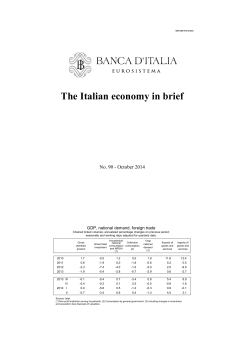


© Copyright 2026