International Journal of Energy and Power Engineering
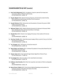
2014; 3(5): 266-276
Published online November 21, 2014 (http://www.sciencepublishinggroup.com/j/ijepe)
doi: 10.11648/j.ijepe.20140305.18
ISSN: 2326-957X (Print); ISSN:2326-960X (Online)
State estimation of the Tanzanian power system network
using non-quadratic criterion and MATLAB environment
Mashauri Adam Kusekwa
Electrical Engineering Department, Dar es Salaam Institute of Technology,Dar es Salaam, Tanzania
Email address:
[email protected], [email protected]
To cite this article:
Mashauri Adam Kusekwa. State Estimation of the Tanzanian Power System Network Using Non-Quadratic Criterion and MATLAB
Environment. International Journal of Energy and Power Engineering. Vol. 3, No. 5, 2014, pp. 266-276.
doi: 10.11648/j.ijepe.20140305.18
Abstract: Power system state estimation is an effective online tool for monitoring, control and for providing consistent
database in energy management systems. This paper presents an algorithm for state estimation of the Tanzanian power system
network using a non-quadratic state criterion. Equality and inequality constraints existing in a power system are included in
formulating the estimation problem. Equality constraints are target values used in load flow analysis and are included in power
system state estimation in order to restore observability to those parts of the power system network which are permanently or
temporarily unobservable. Inequality constraints are limits such as minimum and maximum reactive power generation,
transformer tap and phase-shift. The solution techniques used is primal-dual interior point logarithmic barrier functions to treat
the inequality constraints. An algorithm is developed using the method and a program coded in MATLAB is applied in
implementing the simulation. Computational issues arising in the implementation of the algorithm are presented. The
simulation results demonstrate that the primal-dual logarithmic barrier interior point algorithm is a useful numerical tool to
compute the state of an electrical power system network. The inequality constraints play essential role in enhancing the
reliability of the estimation results. Also, it is expected that significant benefit could be gained from application of the
constrained state estimation algorithm to the Tanzanian power system network.
Keywords: Power Systems, Non-Quadratic State Estimation, Simulation, Interior Point Method, MATLAB Program
1. Introduction
Power system state estimation is a mathematical procedure
[1] which processes a set of real-time measurements such as
voltages, real and reactive power injections, real and reactive
power flows using the topology determined by the topology
processor to come out with the best estimate of the current
state of the power system. The state of a system is defined as
a vector of the voltage magnitude and voltage angle of each
bus of that system.
Power system state estimation is important for control and
security monitoring of a system. Using real-time system
measurements, it is easy to identify whether the system is
normal or not. In addition, the state estimator is used to build
the model for the observable part of the network [2]. It is
used to filter redundant data [2-3] to eliminate incorrect
measurement, and to produce reliable state estimates.
Before any control action can be taken or security
assessment can be made, a reliable estimate of the current
state of the system must be determined. For this purpose the
number of physical measurements cannot be restricted to
only those quantities required to support the load flow
computations. The input to the load flow studies is confined
to real and reactive power injections at load buses, and real
power and voltage magnitude at voltage-controlled buses. If
one of these inputs is unavailable, the load flow solution
cannot be determined. In addition, gross-error in one of the
input quantities can cause the load flow solution to be useless.
In practice, other conveniently measured quantities such as
real and reactive power flows are available, but they cannot
be used in the load flow program. These limitations can be
removed by state estimation.
The main objective of the state estimator is to find best
estimate of unknown voltage angle at every bus in the
modelled system network [4]. Since inexact measurementssuch as those from SCADA system are used to calculate the
state vector, the estimate will also be inexact. This introduces
the problem of how to device the best estimate for the state
International Journal of Energy and Power Engineering 2014; 3(5): 266-276
vector given the available measurements.
The results from state estimation provides the real-time
database [1],[3] for other network applications such as
security assessment, determination of power flows in parts of
network that are not directly metered, optimal power flow,
contingency analysis, etc. State estimation can also be used
for data validation. One of the major benefits of state
estimation is its ability for detection and identification of bad
data.
The technical literature is rich pertaining to power system
state estimation. The pioneering work is due to Schweppe et
al [5-7]. The first practical implementation of state estimator
is reported in [8]. The model for state estimation problem is
well established and diverse solutions are also well known.
Appropriate background information on power system state
estimation can be found in [9], [2], and [10].
Particularly interesting is the work by Abur et al [11-12].
The work reported in [11] implements a fast algorithm for the
weighted least absolute value (WLAV) state estimation using
simplex method. WLAV fall under non-quadratic criterion.
This work is extended in [12] to include equality and
inequality constraints on measurements. Incorporating of
constraints in formulating state estimation problem enhances
the reliability of the estimator. In all the described work the
state estimation problem is formulated as a linear
programming (LP) problem and solved by using simplex
method. Interest of using interior point method is described
in the work of Clements et al [13]. Application of interior
point method is extended in [14-15]. The work reported in
[13], [14] is different from the work described in this paper.
In [13] logarithmic barrier function is directly used in solving
the problem. In [14] the authors formulated the state
estimation problem as an optimization problem and used the
barrier function method in solving the primal formulation and
affine scaling method in solving the dual formulation of the
problem.
In this paper, the problem is set up as an optimization
problem with a linear objective function subject to a set of
non-linear constraints resulting from the measurement errors.
Primal-dual logarithmic barrier path following method is
applied in solving the constrained non-quadratic state
estimation problem. This approach is computationally
extremely useful because the principal computational step in
solving the symmetric positive semi-definite system is
identical to that of solving unconstrained weighted least
squares (WLS) problem. Consequently, this method is
implemented using modified WLS MATLAB software.
The paper is organized as follows. Section 2 presents
Tanzanian power system network generation and high
voltage transmission system status. The system is used as a
case study in testing the non-quadratic state estimation
algorithm. Section 3 gives material and method followed by
problem formulation in which measurement model, least
absolute value (LAV) state estimation formulation, nonquadratic constrained state estimation problem and algorithm
are presented.
In section 4 a method of solving the non-quadratic
267
estimation problem using primal-dual logarithmic barrier
path following method is presented. Section 5 presents input
data, simulation procedures and results. Section 6 discusses
the obtained results and section 7 concludes the paper.
2. Tanzanian System Network
2.1. Generation
The Tanzanian power system comprises of hydro, thermal
and isolated thermal generation plants [16]. The hydro
system is comprised of 6 plants with a total nameplate of
561MW (See Table 1). The installed capacity of thermal
generating plants totals 453.6MW. The installed capacity of
isolated thermal generating plants totals 38.45MW. Currently,
the total nameplate capacity is 1,053.05 MW [16]. The
demand for electricity in Tanzania is growing at a relatively
fast rate (See Table 4). The annual average load growth rate
between 1990 and 1998 was 5 percent; the average load
growth rate between 2003 and 2006 has been above 11
percent [17]. This load growth rate has been achieved despite
long period of load shedding due to drought and inadequate
water and rainfall in the main hydropower reservoirs and
their catchments areas.
Tanzania Electric Supply Company Limited (TANESCO)
owns all of the hydro generating plants in the country and
some of the thermal generating plants, although there are
some independent power producers (IPPs) owned by private
operators. Tables 1 and 2 show the installed grid connected
generation capacities for the country. The system presently
consists of an interconnected grid and several isolated
systems. The model of the interconnected grid is shown in
Figure 1. The interconnected system consists of hydro and
thermal generating plants providing power to Cities,
Municipals and Townships.
Table 1. Installed hydro grid generation capacity
Plant Name
Kihansi
Kidatu
Mtera
NPF
Hale
NYM
TOTAL
Fuel Type
Hydro
Hydro
Hydro
Hydro
Hydro
Hydro
Installed Capacity [MW]
180.00
204.00
80.00
68.00
21.00
08.00
561.00
Ownership
TANESCO
TANESCO
TANESCO
TANESCO
TANESCO
TANESCO
Table 2. Installed thermal grid generation capacity
Plant Name
Songas
Ubungo
IPTL
Dodoma
Mbeya
Mwanza
Musoma
Tabora
TOTAL
Fuel Type
Natural gas
Natural gas
HFO
IDO
IDO
IDO
IDO
IDO
Installed Capacity [MW]
202.00
102.00
103.00
07.44
13.90
12.50
02.56
10.20
453.60
Ownership
Private
TANESCO
Private
TANESCO
TANESCO
TANESCO
TANESCO
TANESCO
Source: Economic Survey Report: 2007 and 2009 IDO – Industrial Diesel
Oil, HFO- Heavy Fuel Oil
268
Mashauri Adam Kusekwa: State Estimation of the Tanzanian Power System Network Using Non-Quadratic Criterion and
MATLAB Environment
Figure 1. Tanzanian network model
2.2. Transmission Network
TANESCO owns high voltage and low voltage
transmission and distribution lines of different voltage levels
scattered all over the country. The high voltage transmission
lines (See Table 3) are estimated to comprise of 2,624.36 km
of system voltage 220 kV; 1,441.50 km of 132 kV and
486.00 km of 66 kV, totalling to 4,551.86 km by the end of
December 2006 [16]. High voltage transmission lines use
pylons made of steel. Almost all HV transmission lines are
radial single circuit lines. The country power system is
alternating current (AC) and the system frequency is 50 Hz.
The TANESCO grid comprises of: South-West grid, NorthWest grid and North-East grid. South-East grid is still under
planning stage.
South-West grid mostly of 220 kV connects: UbungoMorogoro-Kidatu-Kihansi-Iringa-Mufindi-Mbeya.
NorthWest grid connects: Ubungo-Morogoro-Kidatu-KihansiIringa-Mtera-Dodoma-Singida-Shinyanga-Mwanza (220 kV);
Mwanza- Musoma (132 kV)-Shinyanga- Tabora (132 kV)
North-East grid connects: Ubungo-Tegeta-Zanzibar (132 kV);
Ubungo-Chalinze- Hale-NPF-Tanga (132 kV); Chalinze –
Moshi – Arusha (132 kV); NYM – Moshi (66 kV); ArushaBabati-Singida (220 kV).
3. Material and Method
Electrical data used in this study were obtained from
Tanzania Electric Supply Company Limited (TANESCO). A
computer software programme, MATLAB was used to
determine the state vector of the Tanzania Power Electrical
Network.
3.1. Problem Formulation
3.1.1. Measurement Model
The mathematical measurement model of state estimation
is based on the mathematical relations between the
measurement and the state vector given by:
z = h( x ) + r
(1)
Where
z ∈ ℜ mx1 Is the vector of measurements i.e. the voltages,
injection powers and flow powers
x ∈ ℜ 2 N −1 is the vector of state variables
h(.) ∈ ℜ mx1 is the non-linear function relating the
measurement to state vector
r ∈ ℜ mx1 is the measurement residual vector
N is the number of buses
m is the number of measurements
n = 2 N − 1 is the number of state vector components
International Journal of Energy and Power Engineering 2014; 3(5): 266-276
269
The measurement system consists of real and reactive
power injections, real and reactive line power flows and bus
voltage magnitude.
ε k ,P
is the error corresponding to real power injection
ε k ,Q
is the error corresponding to reactive power
3.2. Least Absolute Value (LAV) State Estimation Criterion
injection
The least absolute value (LAV) state estimation problem
criterion is formulated as:

mk ,V V meas −V est
k
k,


+


σ k2,V
k =1



 mk ,Pinj Pmeas − Pest
k ,Pinj
k,Pinj
+

+
2


σ k, pinj

 k=1

 mk ,Q
meas
est
N
inj Q
k,Qinj − Qk,Qinj 

minJ (V∠δ ) = +
+
σ k2,Qinj

i=1  k=1


est
 mk ,Pflo Pkmeas

,Pflo − Pk ,Pflo

+
+

 k=1
σ k2, p flo


 mk ,Q flo Qmeas − Qest 
k ,Qflo
k,Qflo

+
2


σ
k,Qflo

 k=1
∑
∑
∑ ∑
(2)
∑
The objective of the estimator is to minimize the errors in
order to get a best estimate of the system. In this way
equation (2) is transformed into:
∑
∑ ∑
∑
∑
∑






+






mk ,V ∈ ℜ
flo
is the error corresponding to real power flows
ε k ,Q is the error corresponding to reactive power flows
δ : Voltage angle (unknown variable)
σ : Standard deviation
flo
J : Objective function
The state estimator needs a set of analogue measurements
and system topology to estimate the system state. The
minimal measurement number required is equal to (2N-1) the
dimension of the state vectors. Hence, the critical number of
real and reactive measurement pair is (N-1) with addition of
voltage magnitude measurement.
The non-quadratic constrained state estimation problem is
formulated by including equality and inequality constrains
existing in the system. Equality constraints are target values
used in load flow analysis and are included in power system
state estimation in order to restore observability to those parts
of the power system network which are permanently or
temporarily unobservable. Equality constraints can be treated
as pseudo-measurements with relative high weights [18].The
equality constraints are the power balance equations which
are described in Momoh [19] as:
N
q=1
is the number of voltage magnitude
(4)
p =1, N
(3)
Qp −Vp ∑Vq(Gpqsinδpq − Bpqcosδpq) = 0
N
q=1
(5)
p =1, N
Where
p is not a slack bus, and
δ slack = 0
Pp , Q p is the real and reactive power injection at bus p
measurement
mk , Pinj ∈ ℜ
ε k ,P
Pp −Vp ∑Vq(Gpq cosδpq + Bpq sinδpq) = 0
Where
N
inj
3.3. Constrained State Estimation Problem
∑
mk , Pinj
mk ,V ε
εk,Pinj
k ,V

+
+
 σ2
σk2,Pinj
k,V
k
=
1
k
=
1

 mk,Qinj
N
εk,Qinj mk ,Pflo εk,Pflo

minJ (V∠δ ) = +
+
2
2
i =1  k =1 σk,Qinj
k =1 σk , Pflo
 m
 k,Q flo εk,Qflo
+
 k =1 σk2,Qflo

inj
N
is the number of real power injection
measurement?
mk ,Qinj ∈ ℜ N is the number of reactive power injection
measurement
m k , Pflo ∈ ℜ 2 N is the number of real power flows
measurements
mk ,Q flo ∈ ℜ 2 N is the number of reactive power flows
measurements
ε k ,V : is the error corresponding to voltage magnitude
V p ∠δ p is the voltage at bus p
δ pq = δ p − δ q
G pq + jB pq Are the corresponding elements in system
bus admittance matrix
The power injection at bus p is defined as
Pp = PGp − PLp
(6)
Q p = QGp − Q Lp
(7)
270
Mashauri Adam Kusekwa: State Estimation of the Tanzanian Power System Network Using Non-Quadratic Criterion and
MATLAB Environment
Where
PGp , QGp
Are the real and reactive power generation at
bus p, while PLp , Q Lp are the real and reactive load power at
bus p. Bus voltage magnitude including the slack bus, and
bus voltage angles except the slack bus where δ slack = 0 are
taken as state vector x.
Inequality constraints are limits such as minimum and
maximum reactive power generation, transformer tap and
phase-shift limit
The constraints are initially relaxed as one approach to the
solution and those constraints that are violated are enforced
on the corresponding limits either as equality constraints with
relative high weights. Interior point methods have been
suggested in relaxing the constraints as proposed in [20]
Therefore, the aim of this paper is to minimize the errors
given in (3) by considering all constraints existing in the
system network. Normally, in the weighted least squares
(WLS) estimators, the influence of a measurement on the
state estimate increases with the size of its residual while
non-quadratic estimators (LAV/WLAV) are designed to
bound the influence of large residuals on state estimation
with prediction that these residuals correspond to gross error
measurements. With this idea in mind, in this paper a nonquadratic criterion is used in developing the method and
algorithm for solution of estimation problem.
In this way the non-quadratic constraint weighted least
absolute value (WLAV) state estimation is formulated as
follows:
min[diag R −1 ]T z − h( x )
( )
(8)
ε = z − h( x )

Subject to  g ( x ) = 0
ε ≥ 0

(9)
Where
diag ( R −1 ) = W is the weighting factor
4. Solution Method
4.1. Primal-Dual Interior Point Methods
Interior point methods (IPMs) for non-linear programming
problems have been studied since the early 1950s by Fiacco
and McCormick [21]. Interest in interior point method was
rekindled by introduction of projective method by Karmarkar
in 1984 [22]. Karmarkar’s method was equivalent to an
interior point method known as the logarithmic barrier
function method. In this method, the inequality non-linear
constraints in (10) can be converted to equality non-linear
constraints by adding non-negative slack variable vectors (u,
l≥0).
To ensure that these slack variable vectors will remain
positive, the logarithmic barrier function is appended to the
objective function of eqn (10). Then the state estimation
problem (10) is transformed to a problem with equality
constraints (11), which can be written as:
m
min W T ε − µ ∑ (ln u k + ln l k )
k =1
− ε − r + u = 0
− ε + r + l = 0

s.t. g ( x ) = 0
r − z + h ( x ) = 0

(ε , u, l ) ≥ 0
(11)
Where
µ> 0 is the barrier parameter. It value is forced to decrease
towards zero as the iterations progress.
m is the number of rows of measurement vector z
u k , l k : are the kth elements of the slack variable vectors u
and l
The Lagrangian function of the problem (11) is defined as:
z − h(x ) = ε ∈ ℜ mx1 is the measurement error vector
The measurement error vector is of the whole system as
given by equation (3).
g : is the non-linear vector function of the equality
constraints.
Since it is difficult to solve Eqns (8) and (9) directly, the
problem is transformed to the following equivalent problem
as:
min W T ε
r − ε ≤ 0
− r − ε ≤ 0

s.t. g (x ) = 0
r − z + h ( x ) = 0

ε ≥ 0
The solution technique employed is solving the nonquadratic constrained estimation problem is a primal-dual
logarithmic barrier path following interior point method.
(10)
L = W Tε −
m
∑ (ln u
k
+ ln lk ) − λT [−ε − r + u ] −
k =1
T
(12)
− β [ −ε + r + l ] − η T [r − z + h(x )] − γ T g (x )
Where
λ,β,η, and γare vectors of Lagrange’s multipliers
The Karush-Kuhn-Tucker (KKT) first order necessary
conditions for an optimal solution of the sub-problems of (12)
can be expressed in terms of a stationary point of the
Lagrangian function are given by
∇ u L = − µU −1e − λ = 0
(13)
∇ l L = − µL−1e − β = 0
(14)
International Journal of Energy and Power Engineering 2014; 3(5): 266-276
∇ε L = W + λ + β = 0
(15)
∇λ L = ε + r − u = 0
(16)
∇β L = ε − r − l = 0
(17)
∇r L = λ − β −η = 0
(18)
∇ γ L = − g (x ) = 0
(19)
∇η L = − r + z − h ( x ) = 0
(20)
∇ x L = −H η − G γ = 0
T
T
l1
0
L=
0

0
0
0 
⋱ 0

0 um 
0 ⋯
u2 ⋯
0
0
0
l 2 ⋯ 0 
0 ⋱ 0

0 0 lm 
(23)
Let e = [1, 1, 1] : a vector with all its elements equals to
one.
The KKT non-linear equations can be solved using
different methods. They can be solved either as all equations
together or by reducing them by elimination of variables. In
this paper, the equations are solved iteratively using the
Newton-Raphson method. In this method, the following
linearizing approximations are made at each iteration.
h(x ) ≈ h x + H∆x
k
−1
k −1
k −2
k −2
{(U
µ
0. 5
) + (L ) }
(26)
0.5
µ
k 2
k 2
(U )
k 2
(27)
The solution of Eqn (25) is used to calculate the direction
of changes inβ,γand x. It may not be possible to take a full
Newton-Raphson step without violating the inequality
constraints [23-24]. Hence, the new values ofβ,τ, and x are
computed from:
x k +1 = x k + α P ∆x
γ k +1 = γ k + α D (γ − γ k )
(28)
αP and αD are scalars known as primal and dual step length.
An advantage of using primal-dual method is that of using
two step lengths, one for primal variables and the other for
dual variables
In practice equality constraint measurement are error free,
in this way the equality constraints component in equation
(25) is neglected; this transforms the equation into
H   β   − TW 
=
0  ∆x  − H T W 
 D
2 H T

(29)
∆x can be computed from the following equation
2HT D−1H∆x = 2HT D−1TW− HTW
[
∆x = 2HT D−1H
(30)
] (2H D TW − H W)
−1
T
−1
T
(31)
4.2. Updating and Adjusting the Variables
Assuming that an initial starting point in the interior of the
feasible region is known, and then the solution is updated in
this way:
k
k −1
D = diag
(22)
T
−1
(25)
β k +1 = β k + α D (β − β k )
0 ⋯
( )
g ( x ) ≈ g (x ) + G∆x
U e ≈ (U ) e − (U ) du
L e ≈ (L ) e − (L ) dl
H ≈ H (x )
G ≈ G (x )
( )
Where
D is a diagonal matrix given by
(21)
Where
H and G are Jacobian matrices of h(x),g(x).
U and L are diagonal matrices defined by slack variables u
and l, respectively given by equations (22) and (23) as:
u1
0
U =
0

0
0 H β   −TR−1 
 D


 0
0 G γ  =  − g xk 

2HT − GT 0 ∆x − HT R−1 
T=
(λ , β ) ≥ 0
271
(24)
k
k
After these approximations are made and du and dl are
eliminated, the following system of equations results:
x k +1 = x k + α P dx
u k +1 = u k + α P du
l
k +1
(32)
= l + α P dl
k
λk +1 = λk + α D dλ
β k +1 = β k + α D dβ
(33)
The step length α is choosen such that the solution remains
within the feasible region i.e. u > 0 and l > 0 . In order to
272
Mashauri Adam Kusekwa: State Estimation of the Tanzanian Power System Network Using Non-Quadratic Criterion and
MATLAB Environment
keep
u k +1 ≥ 0 :
u k +1 = u k + α u du > 0
Then
 u k

, du < 0
 du

α u = min −
(34)
Similarly
To keep
l k +1 ≥ 0 :
l k +1 = l k + α l dl > 0
Then
 l k

, dl < 0
 dl

α l = min−
(35)
In this way the step length is choosen using the following
condition
α = τ (1, α u , α l )
(36)
τ is a scalar constant. The scalar constant value is set at
0.9995 in order to prevent the state estimation to be close to
the feasible boundary. In the same way step length α is
appropriately choosen in order to make xk+1 remains interior
to the feasible region. The iteration is performed until the
norm [25] of ∆x becomes less than the pre-defined tolerance
i.e.
∆x ≤ ε tol
µ=
2m
5. Simulation and Results
5.1. Input Data
However, care should be taken when adjusting the barrier
parameter because the parameter is linked to diagonal matrix
D. if barrier parameter becomes zero, the diagonal matrix D
becomes singular and the whole matrix of equation (30)
becomes singular and the solution cannot be found. Therefore,
the barrier parameter should be appropriately adjusted and it
should be close to zero but not equal to zero when x
approaches the optimal solution. At each iteration the
complementary gap is used to adjust the barrier parameter
and is choosen as proposed in [15] i.e.
λT u + β T l
flow results. The second part deals with computation of
variables and implementation of the algorithm. The full
algorithm is given as:
PART I: Initialize:
Initialize k = 0.
x0= flat start using values obtained from the load flow
program
r0 = z-h(x0)
ε0 = z-h(x0)
u0 = ε0 + r0
l0 = ε0 – r0
γ = 0; τ = 0,λ =- 0.5ε, β = -0.5ε
PART II: Calculation and implementation
i Calculate the Jacobian matrix H
ii Calculate the transpose matrix HT
iii Calculate the complementary gap
iv Calculate the barrier parameter (µ)
v Calculate D
vi Calculate du = ε +r - uk
vii Calculate dl = ε - r + lk
viii Calculate lk and uk
ix Calculate rk = z-h(xk)
x Solve ∆x
xi Calculate step length
xii Update xk+1 = xk +α∆x
xiii Check ifz-h (xk+1) <0.0001 if yes STOP. Otherwise
go to III
xiv Update λand β
xv Update u and l
xvi Check convergence criteria
If optimum TERMINATE the procedure. Otherwise update
k = k+1 and go to III
(37)
4.3. The Algorithm
The complete non-quadratic state estimation algorithm
which uses primal-dual logarithmic barrier method in solving
the state estimation problem is presented as follows. The
algorithm has two parts. The first part is concerned with
initialization procedure. Initial values are obtained from load
Voltage magnitude, real and reactive power injections, real
and reactive power flows models are used for solving the
state estimation problem. These models are written as:
zi = Vi + ε i ,V
zi ∈ ℜ N i = 1, N
zi , inj = hi , inj (V∠δ ) + ε i ,inj
zi ∈ ℜ 2 N i = 1, N
(38)
(39)
zi , flow = hi , flow (V∠δ ) + ε i , flow
zi ∈ ℜ
m flow
i = 1, m flow
(40)
Voltage magnitude, real and reactive power injections, real
and reactive power flows measurements are obtained from
the load flow program and are accepted as true measurement
values of the system.
Input data for simulation of the developed algorithm is
given in Tables 3 and 4. Table 3 gives transmission line data
of the Tanzanian Power System Network. Table 4 gives load
International Journal of Energy and Power Engineering 2014; 3(5): 266-276
demand and generation of each bus. Input data for IEEE 14,
IEEE30 bus test systems are obtained from [26].
Table 3. Line data 30-Bus Tanzania System Network
From
To
Impedance
1
2
1
2
2
3
5
6
6
7
8
9
9
10
12
13
13
14
13
16
17
18
20
20
21
22
23
22
25
25
26
27
29
2
3
5
5
24
4
6
7
8
12
9
10
12
11
13
14
15
15
16
17
19
17
19
21
22
23
24
25
26
29
27
28
30
0.012+j0.081
0.020+j0.111
0.039+j0.154
0.025+j0.136
0.016+j0.090
0.034+j0.019
0.014+j0.011
0.00+j0.274
0.018+j0.015
0.086+j0.196
0.00+j0.062
0.043+j0.098
0.010+j0.232
0.052+j0.030
0.018+j0.418
0.009+j0.027
0.063+j0.014
0.049+j0.014
0.026+j0.597
0.00+j0.7373
0.036+j0.716
0.018+j0.037
0.00+j0.1416
0.023+j0.014
0.021+j0.131
0.033+j0.017
0.021+j0.012
0.034+j0.188
0.022+j0.118
0.00+j0.160
0.00+j0.160
0.263+j0.597
0.021+j0.485
Half of line
charging
0.00+j0.065
0.00+j0.085
0.00+j0.122
0.00+j0.010
0.00+j0.068
0.00+j0.143
0.00+j0.087
0.00+j0.00
0.00+j0.117
0.00+j0.020
0.00+j0.00
0.00+j0.00
0.00+j0.024
0.00+j0.00
0.00+j0.043
0.00+j0.00
0.00+j0.00
0.00+j0.00
0.00+j0.062
0.00+j0.00
0.00+j0.00
0.00+j0.00
0.00+j0.00
0.00+j0.111
0.00+j0.100
0.00+j0.137
0.00+0.081
0.00+j0.143
0.00+j0.095
0.00+j0.00
0.00+j0.00
0.00+j0.061
0.00+j041
Tap ratio
setting
1.00
1.00
1.00
1.00
1.00
1.00
1.00
1.00
1.00
1.00
1.00
1.00
1.00
1.00
1.00
1.00
1.00
1.00
1.00
1.00
1.00
1.00
1.00
1.00
1.00
1.00
1.00
1.00
1.00
1.00
1.00
1.00
1.00
Table 4. Busdata 30 -Bus Tanzania System Network
Bus No.
1
2
3
4
5
6
7
8
9
10
11
12
13
14
15
16
17
18
19
20
21
22
23
Load demand
MW
MVAr
06.20
01.60
20.00
07.00
27.00
07.80
18.00
09.10
00.00
00.00
233.10
45.10
17.60
09.00
12.00
02.50
21.00
08.30
23.10
09.00
00.00
00.00
22.00
05.00
00.00
00.00
06.50
01.20
05.00
01.40
06.20
01.60
Generation
MW
14
142.00
259.00
100.00
10.50
68.00
03.60
-
MVAr
-
Bus No.
24
25
26
27
28
29
30
273
Load demand
MW
MVAr
21.70
09.00
29.70
09.60
11.50
05.00
00.00
00.00
05.40
01.50
Generation
MW
74.00
13.00
-
MVAr
-
Table 5. Test systems
No. of buses
No. of lines
No. of measurements
Redundancy
Ward Hale 6
7
25
227.27
IEEE 14
20
41
151.85
30-Bus
33
97
164.41
5.2. Simulation
The prototype code of the non-quadratic constrained state
estimation algorithm was implemented in MATLAB 7.1 and
run on a personal computer having a 3.33GHz Pentium IV
processor and 0.99GB of RAM. Simulations were carried on
using the IEEE 14, IEEE30 test systems and the 30-bus
Tanzanian power system network model. The problem
statistics are summarized in Table 5, where the number of
buses, lines, total number of measurements and redundancies
are given. The measurements were simply chosen such that
the systems become numerically observable. Numerical
observability was checked using the rank (.) function in
MATLAB.
The measurements are simulated adding normally
distributed random error to the load flow results. The
following standard deviations of the measurements are used:
0.004, 0.008, and 0.01 p.u. standard deviations for voltage
magnitudes, line flows and bus injection, respectively. To
verify the accuracy of the resulting estimates, the following
error criteria are calculated according to [12]
∆Vrms =
∆δ rms =
1
N
∑ (V
1
N
∑ (δ
N
p
p =1
N
p =1
p
− V pnon
)
(41)
)
(42)
− δ pnon
Where
V p , δ p : Are the true (load flow solution) voltage
magnitude and phase angle at bus p
non
V pnon
, , δ p : Are the estimates obtained from the nonquadratic state estimator representing the voltage magnitude
and phase angle at bus p.
5.3. Simulation Results
Voltage magnitude and voltage angle profiles are presented
in Table 6. Figures 2 and 3 present voltage magnitudes and
voltage angle profiles in graphical form. The estimation
errors for voltage magnitudes and voltage angles are
274
Mashauri Adam Kusekwa: State Estimation of the Tanzanian Power System Network Using Non-Quadratic Criterion and
MATLAB Environment
presented in Figures 4 and 5, respectively. Figure 6 shows
upper (u) and lower (l) slack variable distribution in
measurements and comparison of measurement residual (r)
and measurement error ( ε ) distribution is presented in
Figure 7.
1.08
1.06
1.04
1.02
1
0.98
P.U.
VOLTAGE MAGNITUDE IN
VOLT AGE MAGNIT UDE PROFILE-T ANZANIA NET WORK
0.96
0.94
0.92
0
10
20
30
40
BUS NUMBER
Figure 2. Voltage magnitude profile-Tanzania Network
Bu
s
No
.
1
2
3
4
5
6
7
8
9
10
11
12
13
14
15
Voltage
Magnitude[p
.u.]
Voltage
Angle[Degr
ee]
00.9614
00.9594
00.9608
00.9548
00.9636
00.9687
00.9579
00.9716
00.9675
00.9545
00.9511
00.9775
00.9715
00.9715
00.9649
00.0000
04.2278
01.7868
01.7692
13.1024
14.3279
19.2351
15.8562
26.6922
30.7587
31.0538
23.1554
27.9832
28.9300
28.5558
Bu
s
No
.
16
17
18
19
20
21
22
23
24
25
26
27
28
29
30
Voltage
Magnitude[p
.u.]
Voltage
Angle[Degr
ee]
00.9350
00.9646
00.9675
00.9605
00.9696
00.9697
00.9494
00.9533
00.9450
00.9989
00.9854
00.9823
00.9443
01.0458
01.0568
14.4283
09.9308
09.9496
02.4502
02.9531
02.9651
03.4359
05.2061
05.8016
-02.6612
-04.5657
-04.4707
-8.6637
-02.3242
-03.7123
The estimation errors for voltage magnitudes and voltage
angles are presented in Figures 4 and 5, respectively. Figure 6
shows upper (u) and lower (l) slack variable distribution in
measurements and comparison of measurement residual (r)
and measurement error ( ε ) distribution is presented in
Figure 7.
VOLTAGE ANGLE PROFILE-TANZANIA NETWOK
40
30
20
10
0
Upper (u) variable distribution
0
-10
10
20
30
1.5
40
u
Upper (u) values
ANGLE IN DEGREE
Table 6. Voltage mag. and Angle profiles of Tanzania System Network
-20
BUS NUM BER
Figure 3. Voltage angle profile-Tanzania Network
1
0.5
0
VOLT AGE MAGNIT UDE ERRORS-T ANZANIA NET WORK
0
20
40
60
80
100
Lower (l) variable distribution
Lower (l) values
ERROR VALUES IN P.U.
0.06
0.04
l
1.5
0.02
0
-0.02
2
0
5
10
15
20
25
30
1
0.5
35
0
-0.04
0
20
40
60
80
Number of measurements (m)
100
-0.06
Figure 6. Upper (u) and lower (l) slack variable distributions
BUS NUMBER
Figure 4. Voltage magnitude errors-Tanzania Network
Residual (r) distribution
1
Value (r)
VOLTAGE ANGLE ERRORS-TANZANIA NETWORK
-1 0
5
10
15
20
25
30
0
35
-1
-2
0
20
-3
40
60
80
100
80
100
Error (e) distribution
-4
1
-5
Value (e)
ERRORS IN DEGREE
0
-6
-7
-8
0.5
0
BUS NUMBER
Figure 5. Voltage angle errors-Tanzania Network
0
20
40
60
number of measurements (m)
Figure 7. Comparison of residual (r) and error distribution
International Journal of Energy and Power Engineering 2014; 3(5): 266-276
6. Discussion
The following observations from simulation results can be
made. The voltage magnitude and voltage angle profiles of
the Tanzanian power system are within acceptable limits i.e.
0.95-1.10 per unit for voltage magnitude and -350-+350
degree for voltage angle. The power factor (pf) of the system
is around 0.857 (+310 degree) which is the accepted
operating value by TANESCO. Voltage magnitude estimation
errors are within pre-defined range of ±5%.
The number of iterations is conditioned by the fact that not
full Newton-Raphson step length (α) for primal variables is
taken in order to remain in the feasible region. If in case
measurements are acting in such way that some of constrains
tend to be violated, the step length is only restricted to some
iterations. The decrease of iterations number is achieved if
more accurate initialization i.e. flats start initialization of
state vector x0is applied.
7. Conclusion
Power system state estimation is a critical function in
determining real-time model for interconnected system
networks. In this environment, a real-time model is extracted
at intervals from snapshots of real-time measurements. It is
generally accepted that the ever expanding system networks
demand network models that are more accurate and reliable
than ever. This can only be achieved with robust state
estimators that reliably deal with state and topology
processing. With that in mind, this paper has presented
development of a non-quadratic state estimation method and
algorithm that incorporate equality and inequality constraints
in its formulation. The simulation results demonstrate that the
primal-dual logarithmic barrier interior point algorithm is a
useful numerical tool to compute the state of an electrical
power system network, when inequality constraints play the
essential role in enhancing the reliability of the estimation
results. Also, it is expected that the significant benefit could
be gained from application of the constrained state estimation
method and algorithm to the Tanzanian power system
network.
Acknowledgement
I would like to thank the Tanzania Electric Supply
Company Limited (TANESCO) for its cooperation and
readiness to supply the most needed data to make this
research work possible. Their support is gratefully
acknowledged.
References
[1]
[2]
F.F. Wu. Real-Time network security monitoring, assessment
and optimization, 9th Power Systems Computation
Conference,Cascais, Portugal,31 August-4 September 1987:
83-100.
A. Monticelli. State estimation in Electric Power Systems: A
275
generalized approach. Kluwer Academic Publishers; Boston,
1999.
[3]
N.H. Abbasy and S.M. Shahidehpour. Application of Nonlinear Programming in Power System State Estimation,
Electric Power Systems Research, 12, 1987:41-50.
[4]
R.E. Larson, W.F. Tinney, and J. Peschon, State Estimation in
Power Systems, part I: Theory and feasibility. IEEE
Transactions on Power Apparatus & Systems; PAS-89(3),
1970: 345-352
[5]
F.C. Schweppe and J.Wildes. Power system Static State
Estimation part I: exact model, IEEE Transactions on Power
Apparatus & Systems; Vol. PAS-89(1); 1970: 120-125
[6]
F.C. Schweppe and D.B. Rom. Power System Static State
Estimation, part II: approximate model, IEEE Transactions on
Power Apparatus & Systems; Vo. PAS-89, (1), 1970: 125-130
[7]
F.C. Schweppe, Power System Static State Estimation part III:
implementation, IEEE Transaction on Power Apparatus &
Systems; Vol. PAS-89(1), 1970: 130-135
[8]
J.J. Allemong, L.Radu, and A.M. Sasson. A fast and reliable
state estimation algorithm for AEP’s new control centre, IEEE
Transactions on Power Apparatus & Systems; Vol. PAS101(3), 1982: 933-944
[9]
L. Holten, A. Gjelsvick, S. Aam, F.F. Wu, and W.H.E. Liu,
Comparison of different methods for state estimation, IEEE
Transaction on Power Systems; 3, (4), 1988: 1798-1806
[10] A. Abur and A.G. Exposito, Power System State EstimationTheory and Implementations. New York: Marcel Dekker, 2004
[11] A. Abur and M. K. Celik, Least Absolute Value State
Estimation with Equality and Inequality Constraints, IEEE
Transactions on Power Systems; 8, (2), 1993: 680-686
[12] A. Abur and M.K. Celik, A fast algorithm for the Weighted
Least Absolute Value State Estimation, IEEE Transactions on
Power Systems; 6, (1), 1991: 1-8
[13] K.A. Clements, P.W. Davis, and K.D. Frey, An interior Point
Algorithm for Weighted Least Absolute Value Power System
State Estimation; IEEE/PES, 91-WM 235-2 PWRS, New York,
1991
[14] H. Singh and F.L. Alvarado, Weighted least Absolute Value
State Estimation using Interior Point Methods. IEEE
Transactions on Power Systems; 9(3), 1994: 1478-1484
[15] H. Wei, H. Sasaki, J. Kubokawa, and R. Yokoyama, An
interior point method for power system weighted non-linear
L1 norm static state estimation. IEEE Transaction on Power
Systems; 13(2), 1998: 17-23
[16] http://www.tanesco.com (May 2012)
[17] http://www.nishati.go.tz (March 2012)
[18] F.F. Wu, and A. Monticelli, A critical review on external
network modelling for on-line security analysis. International
Journal of Electrical Power Engineering Systems, Vol.3, 1983:
222-235
[19] J.A. Momoh, Electric Power System Applications of
Optimization, CRC Press, Taylor & Francis Group, New York,
2009
276
Mashauri Adam Kusekwa: State Estimation of the Tanzanian Power System Network Using Non-Quadratic Criterion and
MATLAB Environment
[20] K.A. Clements, P.W. Davis, and K.D. Frey, Treatment of
inequality constraints in power system state estimation, IEEE
Transactions on Power Systems, Vol. 10, 1995: 567-573
Estimation in Power System State Estimation, “Proceeding of
IFAC int. Symposium on Power System and Power Plant
Control, Seoul Korea, August 22-25, 1989: 785-790
[21] A.V. Fiacco and G.P. McCormick, Non-linear Programming:
Sequential Unconstrained Minimization Technique, John
Wiley & Sons, New York, 1968
[24] K. Chiite and K.S. Swarup, Power System State Estimation
using IP Barrier method, department of Electrical Engineering,
Indian Institute of Technology Madras, 600036 INDIA, 2003:
1-6
[22] N.K. Karmarkar, A new polynomial-time algorithm for linear
programming, Combinatorica 4, 1984: 183-295.
[23] K.A. Clements, P.W. Davis, and K.D. Frey, An efficient
algorithm for computing the Weighted Least Absolute Value
[25] Information
on
norms
obtained
http://www.mathworld.wolfram.com/Norm.html
[26] http://www.ee.washington.edu/research/pstca
from