
d na tr op sn ar tc in or tc el E ec na no se rl ac in ah ce m
Low Temperature Laborator y, Depar tment of Applied Physics
Mika Oksanen
Electronic transport and mechanical resonance modes in graphene
Aalto Universit y
2017
E lectronic transport and
m echanical resonance
modes in graphene
Mika Oksanen
D O C TO R A L
DISSERTATIONS
Aalto University publication series
DOCTORAL DISSERTATIONS 34/2017
Electronic transport and mechanical
resonance modes in graphene
Mika Oksanen
A doctoral dissertation completed for the degree of Doctor of
Science (Technology) to be defended, with the permission of the
Aalto University School of Science, at a public examination held at
the lecture hall Y124 E, otakaari 1 on 24 March 2017 at 12.
Aalto University
School of Science
Low Temperature Laboratory, Department of Applied Physics
Nano group
Supervising professor
Prof. Pertti Hakonen
Preliminary examiners
Dr. Andreas Johansson, University of Jyväskylä, Finland
Dr. Sophie Gueron, Laboratoire de Physique des Solides, Universite Paris Sud, France
Opponent
Prof. Adrian Bachtold, ICFO - The Institute of Photonic Sciences, Spain
Aalto University publication series
DOCTORAL DISSERTATIONS 34/2017
© Mika Oksanen
ISBN 978-952-60-7312-5 (printed)
ISBN 978-952-60-7311-8 (pdf)
ISSN-L 1799-4934
ISSN 1799-4934 (printed)
ISSN 1799-4942 (pdf)
http://urn.fi/URN:ISBN:978-952-60-7311-8
Unigrafia Oy
Helsinki 2017
Finland
Ab s t ra c t
Aalto University, P.O. Box 11000, FI-00076 Aalto www.aalto.fi
Author
Mika Oksanen
Name of the doctoral dissertation
Electronic transport and mechanical resonance modes in graphene
P u b l i s h e r School of Science
U n i t Low Temperature Laboratory, Department of Applied Physics
S e r i e s Aalto University publication series DOCTORAL DISSERTATIONS 34/2017
F i e l d o f r e s e a r c h Nanophysics
M a n u s c r i p t s u b m i t t e d 15 February 2017
D a t e o f t h e d e f e n c e 24 March 2017
P e r m i s s i o n t o p u b l i s h g r a n t e d ( d a t e ) 17 January 2017
Monograph
Article dissertation
L a n g u a g e English
Essay dissertation
Abstract
G rap h e ne i s a t w o - d i me ns io nal s h e e t o f c arb o n a t o ms arrang e d in a h e xag o nal h o ne y c o mb l at t i c e .
After the fi rst electronic devices made from single layer graphene were demonstrated in 2004, a
tremendous interest has arisen around it. It is driven by the unique properties of graphene: it has
a linear band structure so that the charge carriers behave like massless relativistic particles and
very few materials can rival its mechanical, electronic, and optical properties, and most remarkably
they all exist in a single substance. Consequently, graphene has been envisioned to either replace
many currently used materials, or to enable conceptually new applications.
Various aspects of graphene physics and devices has been studied in this Thesis. Transport
experiments were performed on high quality suspended graphene samples, where the intrinsic
performance limits can be probed. At millikelvin temperatures, the ballistic conductance in
monolayer graphene manifests in electron wave interference reminiscent of Fabry-Pérot
resonances in optical cavities. These interference patterns were analyzed to reveal the renormalization of Fermi velocity in graphene at low charge densities. At high bias voltage regime, shot
noise thermometry was employed to study the electron-phonon scattering mechanisms. In
suspended monolayer graphene, hot electron relaxation was found to be dominated by two-phonon
scattering from thermally excited ripples, whereas in bilayer graphene the intrinsic optical phonons
played the dominant role.
Grap he ne is t he u l t imat e mat e rial f or nonline ar, t u nab le t w o-d ime ns ional nanoe l e ct ro me chanic al
systems. In this Thesis, methods to fabricate and measure graphene mechanical resonators were
developed. In addition, diamond-like carbon resonators were studied, which may be a promising
alternative for applications utilizing multilayer graphene membranes.
K e y w o r d s graphene, quantum transport, mechanical resonators
I S B N ( p r i n t e d ) 978-952-60-7312-5
I S S N - L 1799-4934
I S B N ( p d f ) 978-952-60-7311-8
L o c a t i o n o f p u b l i s h e r Helsinki
I S S N ( p r i n t e d ) 1799-4934
L o c a t i o n o f p r i n t i n g Helsinki
I S S N ( p d f ) 1799-4942
Y e a r 2017
P a g e s 149
u r n http://urn.fi /URN:ISBN: 978-952-60-7311-8
Tiivistelmä
Aalto-yliopisto, PL 11000, 00076 Aalto www.aalto.fi
Tekijä
Mika Oksanen
Väitöskirjan nimi
Electronic transport and mechanical resonance modes in graphene
J u l k a i s i j a Perustieteiden korkeakoulu
Y k s i k k ö Low Temperature Laboratory, Department of Applied Physics
S a r j a Aalto University publication series DOCTORAL DISSERTATIONS 34/2017
T u t k i m u s a l a Nanophysics
K ä s i k i r j o i t u k s e n p v m 15.02.2017
V ä i t ö s p ä i v ä 24.03.2017
J u l k a i s u l u v a n m y ö n t ä m i s p ä i v ä 17.01.2017
Monografia
K i e l i Englanti
Artikkeliväitöskirja
Esseeväitöskirja
Tiivistelmä
Grafeeni on hiiliatomeista muodostunut yhden atomikerroksen paksuinen kalvo, jossa atomit ovat
järjestäyneet "hunajakenno" hilaan. Ensimmäiset sähköiset mittaukset grafeenitransistoreilla
tehtiin vuonna 2004, jonka jälkeen kiinnostus grafeenia kohtaan on kasvanut valtavasti. Johtuen
grafeenin hilarakenteesta, sen varauksenkuljettajat käyttäytyvät kuten massattomat Diracin
hiukkaset, ja sen sähköiset, mekaaniset ja optiset ominaisuudet ovat vertaansa vailla. Grafeenin
o nki n aj a t e l t u ko rvaa van mo ni a ny ky i s iä mat e ri aa l e j a mo ni s s a s o ve l l u ks i s s a, s e kä mah d o l l i s t a van
uudentyyppisten elektronisten laitteiden kehittämisen.
Tässä väitöstyössä on tutkittu grafeenin sähköisiä ominaisuuksia sekä grafeenista valmistettuja
mekaanisia resonaattoreita. Varauksenkuljettajien kuljetusilmiöitä tutkittiin korkealaatuisissa
ripustetuissa grafeenitransistoreissa. Hyvin matalissa lämpötiloissa grafeenin varauksenkuljettajat
etenevät pitkiä matkoja siroamatta, mikä näkyy Fabry-Pérot - tyyppisinä resonansseina
johtavuusmittauksissa. Varauksenkuljettajien Fermi-nopeuden renormalisaatiota tutkittiin näitä
resonanssikuvioita analysoimalla. Elektronien ja fononien vuorovaikutusta tutkittiin korkeilla
jännitteillä hyödyntäen shot-kohinaa elektronien lämpötilan määrittämisessä. Yksikerrosgrafeenissa termisesti aktivoituvien fl exuraali-fononien havaittiin vaikuttavan eniten kuumien
elektronien sirontaan, kun taas kaksikerros-grafeenissa optiset fononit olivat päävastuussa
sirontaprosesseissa.
Mekaaniset resonaattorit ovat erittäin herkkiä antureita massan, varauksen, tai voiman
havaitsemiseen. Koska grafeeni on vain yhden atomikerroksen paksuinen, se on ohuin mahdollinen
värähtelevä kalvo. Tässä väitöstyössä kehitettiin menetelmiä grafeeniresonaattoreiden
valmistukseen ja mittaamiseen. Lisäksi tutkittiin timantinkaltaisia hiilikavoja, jotka voivat olla
hyvä vaihtoehto sovelluksissa joissa hyödynnetään monikerros-grafeenikalvoja.
A v a i n s a n a t grafeeni, nanofysiikka
I S B N ( p a i n e t t u ) 978-952-60-7312-5
I S B N ( p d f ) 978-952-60-7311-8
I S S N - L 1799-4934
J u l k a i s u p a i k k a Helsinki
I S S N ( p a i n e t t u ) 1799-4934
P a i n o p a i k k a Helsinki
I S S N ( p d f ) 1799-4942
V u o s i 2017
S i v u m ä ä r ä 149
u r n http://urn.fi /URN:ISBN: 978-952-60-7311-8
Preface
The research presented in this thesis was carried out in the Nano Group
of the Low Temperature Laboratory, Department of Applied Physics at
Aalto University. First I would like to express my gratitude to Prof. Pertti
Hakonen for all the support and guidance during these years, and for the
opportunity to conduct PhD studies in this distinguished laboratory.
The Nano group has offered invaluable support for my research work,
as well as a pleasant working atmosphere. I would like to thank past and
present members of the group: Aurélien Fay, Xuefeng Song, Antti Puska,
Pasi Lähteenmäki, Matti Tomi, Antti Laitinen, Jukka-Pekka Kaikkonen,
Zhenbing Tan, Daniel Cox, Teemu Nieminen, Pasi Häkkinen, Manohar
Kumar, Vitaly Emets, Jayanta Sarkar, and Dmitry Lyashenko. There
where always smart people around me to consult on problems I could
not solve on my own. I must also continue tradition and thank Pasi L’s
car for enabling several extracurricular activities. Somebody somewhere
(probably another struggling PhD candidate) has stated that the PhD is
a "driver’s license" for doing scientific research. At least in this sense I
can say that I have learned a few things about the scientific mindset, and
again the credit for that goes to the people I have worked with.
Additionally, I would like to thank Alexander Savin for a lot of support on various technical issues. I acknowledge Mika Sillanpää, Juha
Pirkkalainen, Jaakko Sulkko, Matthias Brandt, Pauli Virtanen, Andreas
Uppstu, Ari Harju, and Sorin Paraoanu for professional support. Numerous memorable moments were shared with Raphael Khan, Ville Kauppila,
Sergey Danilin, Karthikeyan Sampath Kumar, and Maciej Wiesner. The
administrative staff of the Low Temperature Laboratory also deserves
recognition for all the support they offer to researchers.
Last, I express my gratitude to my wonderful friends and family, especially my parents Mervi and Esko, and Leena and Ilkka, without whom
1
Preface
I never would have made it this far. I believe several lifelong friendships
were forged during my studies of physics. I wish to mention Petteri, Liisa,
Tapani, Jarno, Jan, and Veikko. Finally, I would like to thank my fiancée
Salla for always being there for me.
Helsinki, February 14, 2017,
Mika Oksanen
2
Contents
Preface
1
Contents
3
List of Publications
5
Author’s Contribution
7
1. Introduction
9
2. Fundamentals
11
2.1 Graphene electronic structure . . . . . . . . . . . . . . . . . .
11
2.2 Shot noise . . . . . . . . . . . . . . . . . . . . . . . . . . . . .
14
2.3 Cavity optomechanics . . . . . . . . . . . . . . . . . . . . . . .
16
3. Electronic transport in graphene
21
3.1 Fabry-Pérot resonances in suspended graphene . . . . . . . .
21
3.2 Electron-phonon coupling in monolayer graphene . . . . . .
28
3.3 Electron-phonon coupling in bilayer graphene . . . . . . . .
34
4. Graphene nanomechanics
37
4.1 Stamp transferred resonators . . . . . . . . . . . . . . . . . .
37
4.2 Graphene optomechanics . . . . . . . . . . . . . . . . . . . . .
43
4.3 Diamond-like carbon resonators . . . . . . . . . . . . . . . . .
48
5. Summary
53
References
55
Publications
65
3
Contents
4
List of Publications
This thesis consists of an overview and of the following publications which
are referred to in the text by their Roman numerals.
I Xuefeng Song, Mika Oksanen, Mika A Sillanpää, Harold G. Craighead,
Jeevak M. Parpia, and Pertti J. Hakonen. Stamp transferred suspended
graphene mechanical resonators for radio-frequency electrical readout.
Nano Letters, 12, 198-202, December 2011.
II Mika Oksanen, Andreas Uppstu, Antti Laitinen, Daniel J. Cox, Monica
F. Craciun, Saverio Russo, Ari Harju, and Pertti J. Hakonen. Singlemode and multimode Fabry-Pérot interference in suspended graphene.
Physical Review B, 89, 121414(R), March 2014.
III Antti Laitinen, Mika Oksanen, Aurélien Fay, Daniel Cox, Matti Tomi,
Pauli Virtanen, and Pertti J. Hakonen. Electron-phonon coupling in suspended graphene: supercollisions by ripples. Nano Letters, 14, 30093013, May 2014.
IV Xuefeng Song, Mika Oksanen, Jian Li, Pertti J. Hakonen, and Mika A
Sillanpää. Graphene optomechanics realized at microwave frequencies.
Physical Review Letters, 113, 027404, June 2014.
V Antti Laitinen, Manohar Kumar, Mika Oksanen, Bernard Placais, Pauli
Virtanen, and Pertti J. Hakonen. Coupling between electrons and optical phonons in suspended bilayer graphene. Physical Review B, 91,
121414(R), March 2015.
5
List of Publications
VI Matti Tomi, Andreas Isacsson, Mika Oksanen, Dmitry Lyashenko, JukkaPekka Kaikkonen, Sanna Tervakangas, Jukka Kolehmainen, and Pertti
J. Hakonen. Buckled diamond-like carbon nanomechanical resonators.
Nanoscale, 7, 14747-14751, August 2015.
6
Author’s Contribution
The main contribution of the author in the work presented in this Thesis
is in the experimental part of the results obtained from graphene devices.
The author developed and refined microfabrication techniques for making suspended graphene structures. The author also designed and assembled low-noise measurement systems for mK temperature environment,
including both low frequency and microwave (4-8 GHz) settings.
Publication I: “Stamp transferred suspended graphene mechanical
resonators for radio-frequency electrical readout”
The author fabricated counter-electrode substrates for graphene resonators,
and contributed to the manuscript during its preparation and revision.
Publication II: “Single-mode and multimode Fabry-Pérot
interference in suspended graphene”
The author performed the conductance and shot noise measurements with
Antti Laitinen, participated in the data analysis, wrote parts of the manuscript
and most of the supplement.
Publication III: “Electron-phonon coupling in suspended graphene:
supercollisions by ripples”
The author performed the measurements with Antti Laitinen, took part
in the data analysis and preparation of the manuscript.
7
Author’s Contribution
Publication IV: “Graphene optomechanics realized at microwave
frequencies”
The author took part in the sample fabrication and contributed to the
manuscript during its preparation.
Publication V: “Coupling between electrons and optical phonons in
suspended bilayer graphene”
The author characterized bilayer graphene flakes using Raman spectroscopy
and fabricated suspended devices, performed conductance and shot noise
measurements for the experiment, and took part in the preparation of the
manuscript.
Publication VI: “Buckled diamond-like carbon nanomechanical
resonators”
The author fabricated majority of the samples and characterized the devices using transmission measurements, and compiled the first draft of
the manuscript and the supplement.
Other work the author has contributed to:
Antti Laitinen, G.S. Paraoanu, Mika Oksanen, Monica F. Craciun, Saverio Russo, Edouard Sonin, and Pertti Hakonen. Contact doping, Klein
tunneling, and asymmetry of shot noise in suspended graphene, Physical
Review B 93, 115412 March 2016
8
1. Introduction
Graphene is a single atomic layer isolated from graphite. For a long time
the generally accepted view was that atomically thin films are thermodynamically unstable. No contradicting experimental evidence was found
until the discovery of graphene in 2004 [1]. Experiments with very thin
graphite samples, possibly down to monolayer thickness can be found in
the literature [2, 3], but the work in 2004 by Geim et. al. was the first
unambiguous demonstration of electronic devices made from graphene.
Soon after various other freestanding two-dimensional (2D) crystals were
produced, such as hexagonal boron nitride, MoS2 , WSe2 , etc. [4]. In all
of these materials there exists strong in-plane covalent bonding, but the
layers are held together by weak van der Waals interactions. Remarkably,
single layers from these materials can be extracted via simple mechanical
exfoliation, or the so called "Scotch-tape method". A key finding was also
the weak optical interference effect, which makes single layer crystallites
visible under an optical microscope when placed on a suitable substrate.
Scientific and commercial interest in graphene has grown tremendously
during the past decade. Graphene embodies a number of record-breaking
properties in a one single material. In terms of fundamental physics, the
charge carriers in graphene mimic certain relativistic high energy phenomena, and it is a platform to study many-body interaction effects. Although graphene does not have an intrinsic band gap, its high mobility
makes it immediately attractive for high frequency transistor applications. Graphene is chemically inert and since it is essentially only a surface, it is very sensitive to the ambient environment. Graphene’s high
Young’s modulus and specific strength suggests that incorporating it to
light weight polymers would yield significant improvements in their mechanical performance. At the same time graphene is transparent, so that
various flexible electronic devices can be made. The list can be further
9
Introduction
extended with a very high thermal conductivity, impermeability to gases,
and the capacity to withstand current densities around one million times
higher than copper. It is not hard to see why so much excitement has
arisen around graphene.
The two main themes explored in this Thesis are the electron transport
in high quality graphene devices, and mechanical resonators made from
graphene and related materials. High mobility graphene samples can be
obtained by suspending graphene, which allows to study the intrinsic limits of electron transport without interference from a supporting substrate.
Experiments were performed in high bias conditions, which is a relevant
regime for many practical graphene applications. Mechanical resonators
are very sensitive detectors for mass, force, or charge. As an ultrathin
and lightweigth material, graphene is ideal for nonlinear tunable electromechanical devices. In this Thesis methods to fabricate and measure
graphene mechanical resonators have been developed, which may even
enable the study of quantum mechanical motion of mesoscopic resonators.
10
2. Fundamentals
This chapters describes the basic electronic properties of graphene, and
the main theoretical ideas behind the publications. Extensive reviews of
graphene properties can be found in the literature [5, 6, 7, 8, 9, 10, 11].
2.1
Graphene electronic structure
Carbon is the sixth element in the periodic table with a 1s2 2s2 2p2 ground
state electron configuration. The four valence electrons in the 2s, 2px ,
2py and 2pz orbitals can form various hybridized sp orbitals, which is the
reason why nearly endless different structures can be formed by carboncarbon bonding. In graphene, one 2s orbital is mixed with two 2p orbitals, forming three sp2 hybridized planar σ orbitals with a 120° angle
between them. Consequently, the carbon atoms in graphene arrange in a
hexagonal honeycomb-lattice as shown in Fig. 2.2. The strong σ bond is
responsible for the high mechanical strength of graphene and related carbon allotropes, which can be thought of as being derived from graphene
(Fig. 2.1). The remaining 2pz orbitals are oriented perpendicular to the
graphene surface, and form a delocalized π conduction band.
The lattice vectors in real space are given by
a1 =
a √
(3, 3),
2
a2 =
√
a
(3, − 3),
2
(2.1)
where a = 0.142 nm is the carbon-carbon bond length. The honeycomb lattice consists of a hexagonal Bravais lattice with a two atom basis, which
are denoted by sublattice A and sublattice B. Alternatively, the honeycomb structure can be thought of as a union of two offset triangular lattices. Physically the atoms at sites A and B are the same, but they are
inequivalent in a sense that they cannot be connected by a lattice vector
R = n1 a1 + n2 a2 , where n1 and n2 are integers. The reciprocal lattice is
11
Fundamentals
Figure 2.1. Graphene, the two-dimensional allotrope of carbon can be thought of as the
building block for other nanocarbon structures. Reprinted with permission
from Macmillan Publishers Ltd: Nature Materials [5] ©2007.
also hexagonal as indicated in Fig. 2.2, and the corresponding primitive
vectors in reciprocal space are
b1 =
2π √
(1, 3),
3a
b2 =
√
2π
(1, − 3).
3a
(2.2)
The band structure of graphene was already considered by Wallace in
1947 as a starting point for studying graphite [12]. The band structure
can be well approximated with a tight binding calculation including nearest and next-nearest neighbour hopping. The dispersion relation is given
by
E(k) = ±t 3 + f (k) − t f (k),
where
f (k) = 2 cos
√
3ky a + 4 cos
3
3
ky a cos
kx a .
2
2
(2.3)
√
(2.4)
Here t ≈ 2.8 eV is the nearest neighbour hopping energy between the sublattices [6], and t ≈ 0.1 eV the next-nearest neighbour hopping energy
which is not known very accurately. The band structure is illustrated in
Fig. 2.3. The t term breaks the electron-hole symmetry, but it is usually neglected. The valence and conduction bands touch at the corners of
12
Fundamentals
Figure 2.2. Left: the hexagonal honeycomb lattice of graphene, where the two sublattices A and B are denoted with different colours. The primitive vectors are
indicated as a1 and a2 . Right: The graphene Brillouin zone, which is also
hexagonal. The lattice vectors in reciprocal space are indicated by b1 and b2 .
Reprinted with permission from [6] ©2009 American Physical Society.
the Brillouin zone, which are called Dirac points. Only two of them are
inequivalent, located at
K=(
2π 2π
, √ ),
3a 3 3a
K = (
2π
2π
,− √ )
3a 3 3a
(2.5)
in the reciprocal space. In pristine graphene, the Fermi energy lies at zero
energy where the π bands cross. The effective dispersion relation at small
wavevector k = q + K, with q K can be written as [12]
E± (q) = ±vF |q| + O(q/k)2 ,
(2.6)
where q is the momentum relative to the Dirac point K (or K ). The
energy-momentum relationship in graphene is thus linear for both electrons and holes (Fig. 2.3). Graphene can also be classified as a gapless
semiconductor. The energy of the charge carriers depends on the constant
vF , the Fermi velocity. Its magnitude can be estimated from the tightbinding parameters as vF = 3ta/2 ≈106 m/s in an empty band. It is also
worth to note that the velocity does not depend on the momentum as in
the usual case. The density of states also depends linearly on energy:
ρ(E) =
2Ac |E|
,
π vF2
(2.7)
where Ac is the unit cell area. This result can be contrasted to the constant density of states in ordinary 2DEG systems.
The low energy Hamiltonian for charge carriers close to the Dirac point
has the form
13
Fundamentals
Figure 2.3. The band structure of graphene. The zoom-in near the Dirac point shows the
linear dispersion at low energies. Reprinted with permission from [13] ©2006
AIP Publishing LLC.
⎛
Ĥ = vF ⎝
0
qx − iqy
qx + iqy
0
⎞
⎠ = vF σ · q,
(2.8)
which is analogous to a Dirac Hamiltonian for relativistic massless particles, where the speed of light is replaced by the Fermi velocity. Due to
the two atom basis, the wavefunction has a two component form corresponding to electron densities in sublattice A and sublattice B. This is an
additional degree of freedom dubbed pseudo-spin (or chirality), which together with the linear spectrum gives rise to the many exotic phenomena
only present in graphene such as Klein tunneling [14] or the anomalous
half-integer quantum Hall effect [15, 16].
2.2
Shot noise
Shot noise in electronic conductors is the out of equilibrium noise that is
a result of the discrete nature of charge [17]. In devices such as a vacuum
tube, pn-diode, or a tunnel junction, the charge carriers are transmitted
intermittently in an uncorrelated fashion, i.e. as a Poisson process. The
shot noise is "white", meaning that it does not depend on frequency over a
wide range. This is true for frequencies ω < 1/τ , where τ is the width of a
one electron transmission event. The so called Poissonian noise spectrum
was already derived by Schottky [18]:
SP = 2eI,
14
(2.9)
Fundamentals
where I is the time-averaged current. Shot noise is interesting due to
the reason that it contains information on the temporal correlations of the
charge carriers.
The Landauer-Büttiker formalism is a powerful tool to describe the conductance properties of mesoscopic conductors via the scattering approach
[19]. The conductor is considered as a scattering region which is connected
to two reservoirs, and the conductance at the zero temperature limit can
be written as
G=
e2 Tn ,
h n
(2.10)
where Tn are the transmission probabilities for n = 1...N transmission
channels, which are assumed to be independent of energy. The noise produced by the conductor at temperature T at equilibrium, i.e. voltage V = 0
is given by
SI = 4kb T
e2 Tn ,
h n
(2.11)
which is simply the Johnson-Nyquist noise produced by a resistor [20, 21].
It is evident from Eq. (2.11) that the thermal noise does not contain more
information about the conductor than what is gained from conductance
measurement. However, for a finite voltage V > 0 (T = 0), the shot noise
reads [17]
SI =
e3 |V | Tn (1 − Tn ).
π n
(2.12)
It can be seen that the shot noise is determined by a sum of products between transmission and reflection probabilities. The shot noise vanishes
for a ballistic conductor where Tn = 1. For a system where Tn 1 for all
channels, the Poisson value is recovered:
SP =
e3 |V | Tn ≡ 2eI.
π n
(2.13)
The reduction of shot noise from the Poisson value is typically characterized by the Fano factor F , which is the ratio of actual noise to the Poissonian value:
F =
SI
=
SP
− Tn )
.
T
n n
n (1
nT
(2.14)
The Fano factor F = 0 corresponds to fully transparent channels, and
F = 1 to purely Poissonian noise processes. Eq. (2.12) can be generalized
15
Fundamentals
for finite temperature and finite bias: [22, 23]
SP = 2
eV e2
[2kB T
)
Tn2 + eV coth(
Tn (1 − Tn )].
h
2kB T n
n
(2.15)
Eq. (2.15) describes the crossover from thermal noise (eV << kB T ) to shot
noise (eV >> kb T ).
2.3
Cavity optomechanics
Light can transfer momentum to an object, an effect known as the radiation pressure force. The momentum transferred by a single photon
is Δp = 2k. The effect is normally very weak, but it can be magnified
by confining the electromagnetic field inside a cavity. Canonical optomechanical setup is shown in Fig. 2.4: one of the cavity mirrors is fixed,
while the other one is free to vibrate at a frequency ωm . As a consequence,
the resonance frequency of the optical cavity depends on the position of
the mirror. For instance, this system can be used to interferometrically
measure the position of the movable mirror with great accuracy, as was
done in the search for gravitational waves [24, 25]. The radiation pressure
force in a cavity gives rise to dynamical back-action effects, such as parametric instability (or optomechanical amplification) and optomechanical
back-action cooling of the mechanical motion [26]. The effects are classical and result from the finite lifetime of the photons inside the cavity. The
discrete nature of photons also leads to the so called standard quantum
limit, which imposes constraints on how accurately the mirror position
can be measured.
In recent years, the optomechanical principle has been extended from
macroscopic devices to micro- and nanomechanical systems, and from optical frequencies to microwaves. The long standing goal is to be able to
coherently control the motion of mechanical resonators at quantum level
[27, 28]. To this end high frequency resonators have been studied in a
cryogenic environment, and sideband cooling has been utilized to reach
the mechanical ground state [29, 30].
The basic concepts of optomechanics are reviewed below [27, 28]. For an
optical cavity with length L and N antinodes, the resonance frequency is
given by
fc =
16
c
N c
Nc
ωc
=
=
(1 + x/L),
2π
2L/N
2 L−x
2L
(2.16)
Fundamentals
Figure 2.4. Fabry-Pérot cavity with a harmonically suspended end mirror.
where x denotes the coordinate of the movable mirror. The optomechanical coupling strength describes how much the cavity frequency changes
due to mechanical displacement:
g≡
Here xzp =
ωc
∂ωc
xzp =
xzp .
∂x
L
(2.17)
/2mef f ωm is the mechanical zero-point motion amplitude.
The Hamiltonian describing the coupled system reads
Ĥ = ωc a† a + ωm b† b + ga† a(b† + b),
(2.18)
where a† and b† are the creation operators for the cavity and mechanical resonator, respectively. In the microwave regime, the electromagnetic
mode is confined in a microwave resonator which can be described by an
effective LC circuit. The total capacitance is a sum of a constant C and a
small x-coordinate dependent part Cg (x). The cavity frequency can then
be expressed as
1
1
=
.
ωc = L(C + Cg (x))
LCtot (x)
(2.19)
Following the definition from Eq. (2.17), the coupling strength can written
as
g=
∂ωc
ωc ∂Cg
xzp =
xzp .
∂x
2C ∂x
(2.20)
According to Eq. (2.20), high coupling strength is achieved with a low
total capacitance, large zero-point motion and large change of capacitance
with respect to mechanical motion. For a parallel plate capacitor with a
plate separation d0 , the capacitance sensitivity is ∂Cg /∂x ∝ 1/d20 , which
implies that a small vacuum gap is crucial.
When the microwave cavity is excited with a monochromatic signal ωP
17
Fundamentals
at input power PP , an average photon population is created:
nc =
1
PP κEi
,
ωc (ωP − ωc )2 + ( κ2 )2
(2.21)
where κ = κEi + κEo + κI is the total cavity decay rate including input,
output, and internal decay rates. The photons circulating in the cavity
may interact with the mechanical resonator by Stokes and anti-Stokes
scattering. Since the cavity response curve is a Lorentzian, the preferred
scattering mode depends on the pump detuning Δ = ωc − ωP . For a "red"detuned pump tone below the cavity frequency, the photons are preferably
up-converted by absorbing a phonon from the mechanics, and vice-versa
for a blue-detuned pump. This effectively leads to cooling or heating of
the mechanical motion. The effective optical damping can be written as
γopt = nc g 2
κ
κ
−
κ2 /4 + (Δ + ωm )2 κ2 /4 + (Δ − ωm )2
,
(2.22)
which can be negative or positive depending on the pump detunings. In
the resolved sideband limit where ωm κ, the maximum damping rate
at red-detuned pumping Δ = −ωm is given by
γopt =
4gnc
.
κ
(2.23)
The total effective damping rate is the sum of the optical and intrinsic
mechanical damping (γm = ωm /Qm ) rates:
(2.24)
γef f = γopt + γm .
If the mechanical resonator has an initial thermal phonon occupation
nTm ≈ kb T /ωm , the effective damping reduces the thermal contribution
to
nm =
γm T
n ,
γef f m
(2.25)
assuming the cavity mode is in its ground state. The sideband cooling can
bring the mechanical mode to the ground state, described by nm ∼ 0. This
classical expression does not set a lower limit on the achievable phonon
occupation, but quantum mechanical treatment gives the following restriction:
nm,min =
κ
4ωm
.
(2.26)
For a red-detuned pump at ωP −ωc = ωm the output spectrum at the cavity
18
Fundamentals
center frequency (divided by the system gain G) is given by [31]
γef f
Sout
κEi T κEi
T
=
n +
γopt
2 /4 (nm − 2nc ),
G
κ c
κ
(ω − ωm )2 + γef
f
(2.27)
where nTc is the possible thermal occupation in the cavity. The lower
sideband created around the pump frequency is filtered out by the cavity response function. All the information of the mechanical resonator is
encoded into the sideband signal.
19
Fundamentals
20
3. Electronic transport in graphene
This chapter gives an overview of Publications II, III, and V, in which
electronic transport in graphene was studied.
3.1
Fabry-Pérot resonances in suspended graphene
In ballistic mesoscopic conductors, the charge carriers can interfere similarly to light waves [19]. These Fabry-Pérot type of interference effects are
expected to be rather robust in graphene, due to the very low amount of
disorder present in the material. In suspended, exfoliated graphene samples mobilities up to 106 Vs/cm2 have been reached at low temperatures
[32, 33, 34], which means that graphene devices exhibit ballistic transport
up to micrometer length scales. The transport regimes in a mesoscopic
conductor connected to metallic leads or ’reservoirs’ can be classified according to the momentum and phase relaxation lengths. In a classical
ohmic conductor, both the phase coherence length φ and the mean free
path m are smaller than the conductor length L. The relaxation lengths
are determined by elastic and inelastic scattering. In a diffusive conductor, m < L due to elastic scattering but φ > L, and interference effects
are still observable. The phase coherence length is determined by inelastic scattering. In the ballistic regime φ , m > L and charge carriers fully
retain the wave character and can interfere when propagating between
the contacts. Both φ and m are affected by temperature, and typically
low temperatures are required to see the quantum interference effects.
The conductance of a graphene strip with a length L and width W can
be expressed via the Landauer formalism at zero temperature as
σ0 (E) =
∞
L 4e2 L
G(E) =
Tn (E),
W
W h
(3.1)
n=0
21
Electronic transport in graphene
where the factor 4 accounts for spin and valley degeneracy. The contacts
to the graphene are usually modelled as very highly doped graphene regions. For a high aspect ratio sample with W L, the microscopic details
of the edges are not important. The transmission probabilities are calculated by matching the wavefunctions at the contact edges, and in the
case of graphene there is no requirement for the continuity of the derivative of the wavefunction, as is needed for the Schrödinger equation. The
transmission probabilites are given by [35]
Tn (E) =
Here kn ≡ (vF )−1
E2
E 2 − (vF qn )2
.
− (vF qn )2 cos2 (kn L)
(3.2)
E 2 − (vF qn )2 . The quantization of transverse mo-
mentum qn depends on the choice of boundary conditions, and for infinite
mass confinement it reads qn = (m + 1/2)π/W . Although the density of
states vanishes at the Dirac point, the conductivity remains finite: the
transmission coefficient reads [36]
Tn =
1
,
cosh [π(m + 1/2)L/W ]
2
(3.3)
and the conductivity at zero temperature thus becomes
σmin (μ = T = 0) =
4e2
.
πh
(3.4)
The conductivity at the Dirac point is governed by evanescent modes extending from the leads. The Fano factor at the Dirac point is F = 1/3,
which coincides with the value found in diffusive conductors [36, 37], even
though the transport in pristine graphene is ballistic.
Fabry-Pérot interference has been observed with carbon nanotubes in
several experiments [38, 39, 40]. Consider a 1D conductor connected
weakly to two reservoirs via two barriers. Each barrier is described by
a complex transmission probability Ti = |ti |2 = 1 − Ri = 1 − |ri |2 (i = 1, 2),
and only one conduction channel is taken into account. This toy model
works rather accurately with carbon nanotubes, where only few conduction channels typically play a role. With scattering matrix formalism the
total transmission through the system by one channel can be written as
[41]
T12 =
22
T1 T 2
√
,
1 + R1 R2 − 2 R1 R2 cos(2φ)
(3.5)
Electronic transport in graphene
where φ =
√
2mEL is the dynamic phase of the particle that traverses
the conductor. Eq. (3.5) takes into account the multiple reflections the
particle can undergo while traversing through the conductor. For suitable
energies E the phase factor becomes φ ≈ nπ (where n is an integer), and
the total transmission probability approaches unity, i.e. resonant transmission. This happens also in the case where the transmission probability
for each barrier is very small (Ti 1). For a classical disordered conductor and incoherent transport the phase factor disappears and the total
transmission is the sum of the contribution from individual barriers, as
in the ohmic addition of resistances.
Theoretical studies on Fabry-Pérot resonances in graphene have been
carried out recently [35, 42]. Gunlycke and White have showed that periodic oscillations should be present in conductance measurements [43], so
that the periodicity depends on the dimensions W, L of the sample and the
velocity of the charge carriers vF . Both transversely and longitudinally
quantized modes are present. Experimental signatures of Fabry-Pérot
type resonances have been seen in previous experiments [33, 44, 45, 46],
but the large number of conduction channels present in graphene as well
as possible disorder in SiO2 supported devices complicate the analysis of
the interference patterns.
By solving a particle-in-a-box problem with linear dispersion, the approximate locations for the Fabry-Pérot resonances in energy are given
by [35, 43]
EqL ,qW ∼
=±
2
2 (q
EL2 (qL + δL )2 + EW
W + δW ) ,
(3.6)
where EL ≡ hvF /2L and EW ≡ hvF /2W . The constants δL and δW are
governed by the structure of the edges, and the quantum numbers qW
and qL label transverse and longitudinal modes, respectively. For a device with W/L 1, the longitudinal resonances spaced by EL occur due
to the bunching of modes with low qW , which suggests that these resonances are of multimode nature. Conversely, when considering a fixed qL ,
modes with large qW show resonances spaced by EW . Figure 3.1a shows
the approximate locations of these resonances in a simulated graphene
device.
Tight-binding transport simulations were used to study the appearance
of resonances in a graphene device with dimensions 100 × 24 nm2 , which
has the same aspect ratio as the actual sample. Metallic contacts were
modelled by heavily doped graphene leads with a constant doping of 1.5
23
Electronic transport in graphene
Figure 3.1. (a) Simulated conductance curve, where the dashed lines indicate the longitudinal resonances with qW = 0 and arbitrary qL . The solid lines correspond
to transverse resonances with qL = 0 and arbitrary qW , as given by Eq. (3.6).
b) Simulated differential conductance map. c) Fourier transform of ∂Gd /∂μ
from (b), showing the period of both longitudinal and transverse resonances.
eV. Edge disorder can reduce the amplitude of the resonances, and this
effect was simulated by removing atoms from random locations at the
edges. The current through the device was calculated by Landauer apμ
proach, I = (2e2 /h) μLR T (E − EDirac )dE, where μL(R) is the chemical potential of the left (right) contact, T (E −EDirac ) is the transmission function
and eVbias = μR −μL . The position of EDirac with respect to chemical potentials of the leads is shifted by the gate voltage. During the measurements
the graphene device was biased from one end while keeping the other
contact grounded. As a result, the location of the EDirac is shifted with
respect to the chemical potential of the grounded contact. The shift can
be assumed linear ΔEDirac = xeVbias , where x also takes into account possible contact asymmetry. Consequently, when mapping the conductance
as a function of the source-drain bias and the gate voltage, a diamond-like
pattern emerges as shown in Fig. 3.1b. The pattern is symmetric when
x = 1/2. For quantitative analysis, the constant increasing background
of the conductance can be removed by differentiating it with respect to
chemical potential on the y-axis, and taking the Fourier transform of the
differentiated conductance map. The result is shown in Fig. 3.1c. The
inner dots in the figure correspond to periodicity of EL since it is of higher
energy, and the outer dots correspond to transverse resonances with period slightly below EW .
Our experiments were performed on a two terminal suspended graphene
sample with L = 1.1 μm and width W = 4.5 μm (Fig. 3.2a). The graphene
sheet was contacted by Cr/Au contacts, and suspended by etching away
part of the sacrificial SiO2 underneath the graphene with HF acid. A
heavily doped silicon substrate acted as a back gate. Raman spectroscopy
was used to confirm that the graphene flake was a monolayer [47]. The
measurements were performed at a temperature of 50 mK in cryogen-free
dilution refrigerator. Before the measurements, a high current of 1.1 mA
24
Electronic transport in graphene
Figure 3.2. a) Schematic view of a graphene sample (top), where the graphene is supported by the metallic leads, optical image of a real sample is shown at the
bottom. b) The conductivity of the device plotted against charge carrier density n = Cg (Vg −VgD )/e on log-log scale. The straight line is used to determine
the residual charge density of nr = 0.8·1010 cm−2 . The slope at higher charge
density is close to 1/2, indicating ballistic transport. Inset shows the zero-bias
resistance versus Vg − VgDirac .
was passed through the sample, in order to evaporate polymer residue off
from the graphene surface [48]. The field-effect mobility of graphene can
be expressed as
μf =
σ − σ0
,
n(Vg )e
(3.7)
where σ0 is the measured conductivity at the Dirac point and n the charge
carrier density. The graphene device measured here had a mobility of
μf > 105 cm2 /Vs at charge densities n < 2.5 × 10¹⁰ 1/cm2 .
The measurement system is shown schematically in Fig. 3.3. The low
and high frequency measurement lines are separated by bias tees. The
differential conductance of the graphene device Gd ≡ ΔI/ΔVbias was measured with a lock-in amplifier, by passing a small bias current ΔI at
around 35 Hz through the source-drain and measuring the induced voltage. Additionally, a pure dc bias was introduced through a 0.5 MΩ resistor.
The low frequency signals below 1 kHz are heavily filtered before they are
fed into the sample. The high frequency lines that are used to measure
shot noise at 600-900 MHz band, are connected to a cooled low-noise amplifier through a circulator that is operated as an isolator. Differential
shot noise was measured with another lock-in amplifier by reading the
noise power after a diode detector [49].
The experimental map of the graphene conductivity as function of the
bias and gate voltage is shown in Fig. 3.4a. The gate voltage induces
Cg2 (Vg − VgDirac )2 /e2 + n2r , where Cg is the
a charge density via |n0 | =
gate capacitance per unit area, VgDirac the location of the Dirac point, and
25
Electronic transport in graphene
Figure 3.3. (a) Schematics of the measurement setup. The graphene conductivity is
probed at low frequencies, and shot noise is measured at 600-900 MHz band.
The shot noise from graphene is calibrated against a Al/AlOx /Al tunnel junction, and the noise source can be selected with a switch.
nr the residual charge density due to impurities. The residual charge
density can be estimated from Fig. 3.2b as nr ∼ 8 × 109 cm−2 . At gate
voltages Vg > VgDirac , pn junctions are present due to contact doping, which
enhances the visibility of the Fabry-Pérot resonances [50, 51] (Fig. 3.4a)
Figure 3.4b shows the zoom-in of the boxed region in Fig. 3.4a. A
diamond-like pattern of minima and maxima is present in the conductance, although its visibility is reduced due to the increase of the overall
conductance at higher gate voltage. The charge carrier density has been
converted into a low-bias chemical potential via μ0 = sgn(n0 )vF π|n0 |,
where the linear density of states in graphene is used. The data in Fig.
3.4b corresponds to n0 = 1.1 − 1.8 × 1010 cm−2 . The visibility of the resonances can be improved by differentiating the conductance with respect
to chemical potential, which removes the background slope. The dashed
lines in Fig. 3.4c correspond to a period EW = hvF /2W , where W = 4.5 μm
and vF = 2.4 × 10⁶ m/s. Other parameters are Cg = 47aF/μm2 which is cal-
26
Electronic transport in graphene
Figure 3.4. (a) Experimental differential conductance Gd of the graphene sample. b) A
zoom-in of the boxed region in (a), where the gate voltage has been converted
into chemical potential. The resonance pattern is visible, but superimposed
on a background slope. c) The same map as in (b), but now plotting the differentiated conductivity dGd /dμ0 . The dashed lines are a fit corresponding to
the transverse resonances EW using a Fermi velocity vF = 2.4 × 10⁶ m/s. d)
Fourier transform of c). Using the same vF as in (c), both longitudinal (solid
lines) and transverse (dashed lines) can be fit by using the physical dimensions W, L of the sample. e) Differential Fano factor, showing the presence
of the same resonances as the conductance data. f) Fourier transform of (e),
where the dashed and solid lines are the same as in (d).
culated from a parallel plate approximation, and nr = 9 × 109 cm−2 which
agrees well with the estimate from Fig. 3.2b. The diamond pattern is not
fully symmetric, and the asymmetry is attributed to slightly asymmetric
contacts. The fit gives a small asymmetry of x = 0.58.
For a full quantitative analysis, the Fourier transform of the dGd /dμ0
map in Fig. 3.4c is shown in Fig. 3.4d. The dashed lines are fitted with
the same parameters as in Fig. 3.4c. If the transverse resonances are assumed to have a periodicity slightly below EW as in the simulation, the fitting gives a Fermi velocity of vF 2.8×10⁶ m/s. The solid lines in Fig. 3.4d
are fitted to the longitudinal resonance EL = hvF /2L with the same vF
and with L = 1.1 μm. Hence the Fourier analysis reveals both sets of resonances in the conductance data whose periodicity depends on the physical
dimensions of the sample, and the Fermi velocity is vF = 2.4 − 2.8 × 10⁶
m/s at n ∼ 1 − 2 × 1010 cm−2 . This value is much larger than typically
measured in graphene samples fabricated on SiO2 substrates, where the
typical value is roughly 1.1 ×10⁶ m/s [52, 53]. The measured result is consistent with earlier experiments on cyclotron frequency measurements on
suspended graphene [54], where a Fermi velocity between 2 and 3 × 10⁶
m/s at similar charge density was reported. The increased Fermi velocity
is attributed to unscreened electron-electron interactions in high quality
27
Electronic transport in graphene
graphene. [55].
Shot noise measurements can reveal complementary information on the
conduction properties of low-dimensional systems [40, 56]. Shot noise is
characterized through the differential Fano factor defined by Fd ≡ (1/2e)dS/dI.
Figure 3.4e shows the differential Fano factor versus chemical potential
measured over the same bias range as conductance in Fig. 3.4c. The
Fano factor was also differentiated with respect to chemical potential to
increase the visibility of the resonance spots. Although more difficult to
interpret than the conductance data, the Fourier transform (Fig. 3.4f)
reveals maxima with exactly the same periodicity as the conductance.
There are also additional spots in the Fourier transforms of ∂Gd /∂μ
and ∂Fd /∂μ between the transverse and longitudinal resonance locations.
Universal conductance fluctuations (UCF) occur when phase coherent carriers traverse a disordered conductor, so that the conductance variation
is of the order δG ∼ e2 /h, independent of the sample size or amount of
disorder [57]. Although the measured graphene sample is nearly ballistic, residual impurities may still manifest in UCF, especially close to the
Dirac point. Away from Dirac point, the most likely candidate for additional resonant scatterers are adsorbed hydrocarbons [58, 59, 60]. In
tight-binding simulations, vacancies were used to simulate adatoms in
graphene. The amount of scatterers in the simulations were chosen to
match the measured zero bias variance of conductance fluctuations very
close to the Dirac point. By taking an ensemble average over different
defect configurations, it was shown that extra peaks at various locations
between the Fabry-Pérot resonance spots are formed in the Fourier transform maps. Hence it was concluded (see the supplement of Publication
II) that universal conductance fluctuations may coexist with Fabry-Pérot
oscillations, and their quasiperiodicity yields signatures in the Fourier
spectra.
3.2
Electron-phonon coupling in monolayer graphene
Several sensitive detection schemes in bolometry and calorimetry are based
on the ability to control electron-phonon coupling [61]. The electron-phonon
coupling becomes weak at temperatures of the order of a few Kelvin for
most materials, and under a Joule heat flux to the electron system, a
quasiequilibrium can be reached where the electronic temperature Te may
be significantly higher than the phonon temperature Tph . Understanding
28
Electronic transport in graphene
Figure 3.5. Calculated phonon spectra of monolayer graphene. Reprinted with permission from [65] ©2008 American Physical Society.
carrier transport under these conditions is vital for many applications.
Graphene is expected to have an advantage due to its low heat capacity
that allows fast operation [62].
The graphene lattice has six phonon branches, due to the two atom basis
(sublattice A and B) [63]. Three of these are acoustic branches, and the
other three optical (Fig. 3.5). The out-of-plane atomic vibrations account
for one acoustic and one optical mode, while the other four modes correspond to in-plane vibrations. If the modes are classified according to the
direction of movement of atoms with respect to nearest neighbours, the
modes can be divided into transverse and longitudinal. In other words,
the vibrations are considered with respect to the direction of the A-B
carbon bonds. The in-plane transverse and longitudinal acoustic modes,
along with the out-of-plane transverse acoustic mode are degenerate at
the Γ-point, as well as the in-plane optical modes at higher energies [64].
Near the K-point, the phonon modes are responsible for the Raman ac
tive D and G bands. The G band is also known as the 2D peak due to
its strong dependence on the number of graphene layers [47]. At the Kpoint, the in-plane transverse optical mode is non-degenerate, while the
in-plane longitudinal acoustic and in-plane longitudinal optical modes are
degenerate.
At low temperatures, only acoustic phonons are important in metallic systems and typically the longitudinal modes have the strongest coupling. For graphene the energy of optical phonons is high ∼ 200 meV,
so that they are irrelevant below a few hundred Kelvins [66]. For acoustic phonons in graphene, momentum conservation restricts the maximum
29
Electronic transport in graphene
change in momentum to twice the Fermi momentum 2kF [67, 68, 69]. The
corresponding energy scale ω2kF defines the Bloch-Grüneisen temperature TBG by ω2kF = kB TBG . The Bloch-Grüneisen temperature is rather
low in graphene owing to its small Fermi surface, and it can be electro√
statically tuned via kF ∝ n. Above TBG , only a small portion of the
thermally excited modes participate in scattering.
The acoustic phonon scattering can be assisted by other processes, which
significantly enhance the cooling of the hot electrons. Supercollision cooling [66, 70, 71] takes place via impurity scattering in which case the
full thermal distribution of phonons is available. Scattering from flexural phonons may also enhance the cooling processes compared to acoustic
phonons [72, 73], but extremely clean samples are required for these processes to dominate over supercollision cooling.
The heat flow from the conduction electrons/holes to the lattice can be
characterized by a power law of the form
δ
),
P = Σ(Teδ − Tph
(3.8)
where Σ is the electron-phonon coupling constant and δ specifies a characteristic exponent [61]. Our experiments with suspended monolayer
graphene are performed close to the Dirac point at n < 0.1 − 4.5 · 1011
cm−2 , corresponding to TBG < 42 K for acoustic phonons. At T > TBG , the
scattering of electrons from acoustic phonons leads to δ = 1 or δ = 5, depending whether Te << μ or Te > μ, respectively [69]. On the other hand,
supercollision cooling or flexural two-photon scattering lead to δ = 3 or
δ = 5 for Te < μ or Te > μ, respectively.
The experiments were performed on the same sample as discussed in
Section 3.1, with the experimental setup illustrated in Fig. 3.3. The IVcharacteristics and differential conductance Gd were measured at high
bias to heat the electron system by Joule heating. The temperature of the
electron system was measured by shot noise thermometry. At large bias
eV >> kB T the charge transport in graphene is diffusive with substantial
electron-phonon scattering, and the Fano factor is related to electronic
temperature Te via [74, 75, 76]
F =
where Te ≡ (1/L)
L
0
2kB Te
,
e|V |
(3.9)
dxT (x) is the average electronic temperature. The
noise from the graphene sample was calibrated against a Al/AlOx /Al tun-
30
Electronic transport in graphene
Figure 3.6. a) Thermal transport model of the sample: electrons thermalize to metallic
leads via diffusion and via electron-phonon coupling in series with Kapitza
resistance. b) The high bias shot noise plotted at a few different gate voltages
near the Dirac point.
nel junction with F = 1 [17]. In the large bias experiments, the dilution
refrigerator was operated around 0.5 K.
The high bias shot noise is illustrated in Fig. 3.6b. Close to the Dirac
point, strong initial increase in SI is found, which reflects a clearly larger
Fano factor at small charge densities n ∼ nr than at n >> nr . A different
prefactor in the electron phonon coupling was observed at equal hole and
electron densities, which can be attributed to the presence of pn-junctions
at Vg > VgD . The noise generated by the pn junctions is added to the
local thermal noise at high bias voltage, so that the calculated electron
temperature is higher than in reality. For this reason, only data without
pn junctions was used in the analysis. The contribution from the contact
resistance is also reduced from the data (see supplement of Publication
III).
The Joule heating power dissipated in the graphene electron system is
given by Pe = (V − ΔVcc )I where ΔVcc denotes the total voltage drop
over the contacts ΔVcc = Rc I, where Rc = 40 Ω. The heat flow paths
that balance Pe are illustrated in Fig. 3.6a. When the graphene lattice
is cooled to liquid helium temperatures or below, the inelastic processes
dominate the heat flow from electrons to the lattice above temperatures
Te = 200 − 300 K. The phonon temperature Tph remains below few tens
δ in Eq. (3.8) can be neglected. At lower
of Kelvins [77], and thus Tph
electronic temperatures, the heat flow from the electrons is mainly due
to diffusion to the leads (Wiedemann-Franz regime). The contribution of
the electronic heat conduction was subtracted to obtain P from Pe , which
improves the determination of the characteristic exponent δ.
The power law behaviour of P vs Te is plotted in Fig. 3.7a. The char-
31
Electronic transport in graphene
Figure 3.7. a) The heat flow to phonons P versus electronic temperature Te = F e|V |/2kB .
The solid coloured traces indicate measured data, while dashed lines are fits
to Eq. (3.10) with kF eff = 3 and D = 64 eV. The dotted lines show power
laws with δ = 3 (upper) and δ = 5 (lower). b) Total sheet resistance R =
(V /I)W/L as a function of the electronic temperature at n = 0.8 · 1011 cm−2 .
The solid line is fitted as R = [1390 + 0.01(Te /K)2 ] Ω. c) Electron-phonon
coupling power as a function of the charge carrier density at temperatures Te
= 150, 200, and 250 K for Vg < VgD . The solid and dashed lines are obtained
from Eq. (3.10) with same parameters as in a), but with expansions at μ >>
kB Te and μ << kB Te , respectively.
acteristic exponent is determined as δ 3 − 5 depending on the chemical
potential μ = 10 − 73 meV. Close to the Dirac point at |Vg − VgD | < 0.6
V δ = 5, while at at |Vg − VgD | > 5 V, δ = 3 was observed. At intermediate gate voltages 0.6 V< |Vg − VgD | < 5 V, a crossover from δ = 5 to
δ = 3 takes place. The crossover threshold takes place when the electronic system starts to become degenerate (kB Te /μ < 1), which happens
when the chemical potential reaches 20 meV. The observation δ = 5 at
μ << kB Te is consistent with single acoustic phonon scattering at high
temperatures, however, the δ = 3 contradicts this scenario [69, 78]. The
strength of the observed electron phonon-coupling is too high unless an
unrealistically large deformation potential is used, and furthermore the
measured electron-phonon coupling scales quadratically as a function of
the chemical potential (or linearly vs charge carrier density n) whereas
acoustic phonon scattering predicts P ∝ μ0 . Consequently, single phonon
scattering events can be ruled out as the leading contribution to the e-ph
coupling in the suspended sample.
32
Electronic transport in graphene
The electron-phonon heat flow due to supercollisions has been calculated
by Song. et. al. [66]:
Q̇S |Tph =0 −
√
2 k5
gD
N
B 5 vF πn
T
q(
),
k B Te
(2π2 vF2 )2 kF e
(3.10)
where q(z) 9.69 + 1.93z 2 for |z| 5 and q(z) 2ζ(3)z 2 ≈ 2.40z 2 for
|z| 5, and N = 4 is the degeneracy in graphene. The energy dependence of the density of states in graphene leads to cross-over between the
Te3 and Te5 power laws. The electron-phonon coupling constant for defor
mation potential is gD = D/ 2ρs2 where D is the deformation potential,
s is the speed of sound, and ρ the mass density of the graphene sheet.
The dimensionless mean free path kF describes the additional scattering
mechanism that facilitates supercollisions. The Fermi velocity renormalization by electron-electron interactions close to the Dirac point [54, 55]
is also taken into account. Since supercollisions and flexural phonon scattering yield similar power laws, they have to be distinguished by comparing numerical estimates to the data. The ratio of the heat flux via
flexural modes Q̇F to that of supercollision heat flow Q̇S is approximately
Q̇F /Q̇S = kF /200. Equation (3.10) can be fit to the data at |Vg − VgD | > 5
V where it is ∝ Te3 with the parameters vF = 1.0 · 106 m/s (at high energy)
and D/(kF )1/2 = 37 eV. The deformation potential is often estimated in
the range D = 20 − 30 eV [9, 79], which indicates that supercollision cooling is compatible with the results since the heat transfer rate is 100 times
larger than what can be produced by flexural two-phonon scattering. The
electron-phonon heat flow as a function of the charge carrier density at a
fixed temperature is plotted in Fig. 3.7c. The solid lines are fitted using
Eq. (3.10) with the parameters quoted above. The data scales with the
ratio kB Te /μ as predicted by the theory.
Although the graphene sample is nearly ballistic at low bias, the scattering length kF is small at high bias. Contribution of short-ranged impurities or frozen-in ripples is likely small in a high-mobility sample. The
total sheet resistance versus electronic temperature is shown Fig. 3.7b,
from which a temperature-dependent part of the resistivity can be determined as ρi = 0.01(Te /K)2 , which scales quadratically with temperature.
The value is in line with flexural phonon limited mobility analyzed in Ref.
[80] for suspended graphene. If ρi is interpreted as a scattering length
via kF = h/(4e2 ρi ), the scattering length becomes kF ∼ 7 at Te = 300 K,
hinting that an effective scattering mechanism is activated at high bias.
33
Electronic transport in graphene
Flexural phonons, i.e. dynamical ripples can facilitate supercollisions as
is analyzed in Ref. [81]. In this process, a large energy acoustic phonon is
emitted, and the momentum balance is maintained via quasielastic scattering from low energy flexural phonons. An effective kF eff can be obtained from the ρ ∝ T 2 dependence, after adjustments are made for the
characteristic wave vector scales: max(kF , q∗ ) for flexural phonons and
√
qT = kB T /s for acoustic phonons. Here q∗ = us/α is the cut-off of flexural phonons due to strain u in the graphene sheet [34], α = 4.6 · 10−7
m2 /s is specified by the dispersion relation of the flexural modes ω = αq 2 ,
and s = 2.1 · 104 m/s the speed of sound. The strain u ≈ 4 · 10−4 in the
graphene sample was determined from the tuning of the fundamental
flexural mode fres = 77 MHz by the gate voltage: |f − fres | < 0.1 MHz
over Vg = 0 − 10 V. Then the wavevector scales are 2kF < q∗ < qT as in the
regime VI in Ref. [73], and the effective scattering length can be written
as [kF eff ]−1 10(q∗ /qT )2 (4e2 /h)ρi N , where ρi is the T 2 -dependent resistivity component determined above, and N ∝ log(q∗ /qT ) is a factor of the
order unity. The estimate for the scattering length becomes kF eff 3,
which is independent of temperature.
The data in Fig. 3.7a can be fit in the non-degenerate case ∝ Te5 as well
as in the cross-over regime with Eq. (3.10) by using the kF eff determined
above. The fit also indicates D = 64 eV, which is twice the theoretical
estimate D = 20 − 30 eV for the unscreened case [9, 79]. The value of
kF eff is small, but small values due to ripples have been found in STM
studies [82], especially in Ref. [83] kF = 1.8 was measured in a suspended
current-cleaned graphene sample at room temperature.
3.3
Electron-phonon coupling in bilayer graphene
Similar phase space restrictions for the scattering of electrons from acoustic phonons apply for bilayer graphene (BLG) as in the case of monolayer
graphene. On the other hand, since bilayer graphene has a parabolic band
structure, more akin to ordinary two-dimensional electron gas (2DEG)
systems [84], the electron-phonon coupling scales differently with respect
to charge carrier density. The Bloch-Grüneisen temperature in bilayer
BLG = 2(s/v ) (γ |μ|)/k , where γ ≈ 0.4 eV is
graphene is written as TBG
1
1
F
B
the interlayer coupling constant [85]. An approximate numerical value is
given by kB TBG = ω2kF ≈ 18 K × n/1011 cm−2 .
For acoustic phonon scattering, the heat flow can be expressed using the
34
Electronic transport in graphene
S#
L
S1
0.43
0.51
5.8 kΩ
3.0
100 Ω
-0.3V
14000
S2
0.83
3.2
1.5 kΩ
3.6
30 Ω
0.6V
6200
W
R0
σm /σ0
RC
VD
μf
Table 3.1. Summary of the properties for the two samples S1 and S2 presented in the
text. The dimensions are given in μm. R0 and σm are the maximum resistance
2
and minimum conductivity at the Dirac point as multiples of σ0 = 4e
, respecπh
tively. RC is the estimated contact resistance. VD is the location of the Dirac
point in gate voltage. Last column shows the field-effect mobility determined
from the gate sweeps.
form in Eq. (3.8). The experiments with bilayer graphene were conducted
BLG < 34
at low charge densities n < 0.1−3.4·1011 cm−2 , corresponding to TBG
K for longitudinal acoustic phonons. At the high bias regime the results
BLG , where the characteristic exponent is δ = 1
are obtained at T > TBG
or δ = 2, depending whether kB Te << μ or kB Te > μ, respectively [69].
Supercollision cooling due to impurity scattering leads to a similar power
sc
= Asc (Te3 −
law dependence as in the case of monolayer graphene: Pe−ph
3 ) where A is a constant that depends on the mean free path k and
Tph
sc
F
the density of states. The different contributions to the electron-phonon
heat flow are summarized in Fig. 3.8a at n = 1011 1/cm2 . Optical phonons
have the largest contribution at high temperatures, with roughly equal
contributions from long wavelength optical modes around the zone center
(ZC)
(ZE)
(Pe−op , Γ point) and zone edge modes (Pe−op , K point).
The electron-phonon coupling in suspended bilayer graphene was studied using the same methods as in the previous section. The properties
of the two bilayer samples are summarized in Table 3.1. Both samples
were fabricated from exfoliated graphene, and contacted with Cr/Au leads
using EBL. Sample S1 was suspended by etching away sacrificial SiO2 ,
while the sample S2 was suspended using lift-off resist [86]. Both samples
were cleaned by current annealing in cryogenic high vacuum environment
before the measurements.
The Joule heating power Pe dissipated in the bilayer graphene per unit
area as a function of the electronic temperature Te close to the Dirac point
is plotted in Figures 3.8b and 3.8c. At low temperatures, the diffusion
of electrons to the leads at temperature TB dominates the heat flow ac
2 k2 cording to the Wiedemann-Franz law PW F = G π3 eB2 Te2 − TB2 , where G
is the conductance. Above Te = 300 K, an onset to a steeper temperature
dependence is observed, that grows slightly weaker towards higher temperatures. The behaviour can be well accounted for by summing the contributions from Wiedemann-Franz law and the heat flows from coupling
35
Electronic transport in graphene
to the zone center and zone edge optical phonons. At high temperature
(Te = 600 K), the heat flow varies very little as a function of the chemical
potential over the range -12 meV < μ < 12 meV, and the variation can be
explained by the change in Wiedemann-Franz law due to gate dependent
resistance Rd (Vg ). The lack of gate dependence is consistent with both
acoustic and optical phonon scattering, but the strength of the observed
coupling is much higher than what can be produced by acoustic phonons.
Figure 3.8. a) Theoretical estimate for different contributions to the electron-phonon
heat flow in bilayer graphene as a function of the electronic temperature
Te at n = 1011 1/cm2 and Tph = 0. b) Joule heating versus electronic temperature Te = F e|V |/2kB for sample S1 close to the Dirac point at n = 1010
1/cm2 . c) Similar plot for sample S2 as in b). Measured data is indicated
by circles, while the black dashed line illustrates the theoretical expectation
(ZC)
(ZE)
(PW F + Pe−op + Pe−op ). The blue line shows the contribution from the optical
(ZC)
(ZE)
phonons (Pe−op + Pe−op ).
36
4. Graphene nanomechanics
This chapter gives an overview of publications I, IV, and VI, which deal
with graphene and diamond-like carbon mechanical resonators.
4.1
Stamp transferred resonators
Microelectromechanical systems (MEMS) are becoming ubiquitous in various fields of technology , such as automotive, aerospace, instrumentation,
and biomedical industries. MEMS devices typically have integrated electrical and mechanical functionalities, with the feature size of movable
parts are in the micrometer scale. Presently, most MEMS devices are
made from silicon, taking advantage of the existing fabrication technologies for CMOS systems. However, due to the low Young’s modulus, weak
fracture strength, and large coefficient of friction [87], silicon is not the
optimal material for many MEMS applications. In terms of mass density,
mechanical strength, and tribological properties, carbon based materials
can offer greatly improved performance.
The logical miniaturization step from MEMS is to go to the nanometer scale, which is referred to as nanoelecromechanical systems (NEMS).
This size reduction leads to lower mass, higher operating frequency and
increased sensitivity [88]. In addition to their technological potential, nanoelectromechanical (NEM) resonators are the most interesting in terms
of basic research, namely for observing quantum mechanical behaviour
[89, 90, 91, 92]. Graphene is a very intriguing material for NEM resonators. Being only one atomic layer thick, it represents the ultimate
limit of two-dimensional NEMS. It has a high Young’s modulus E ∼ 1 TPa
[93], and together with its extremely low mass, graphene is well suited for
high-frequency mechanical resonators.
Very soon after discovery of graphene, the first monolayer graphene res-
37
Graphene nanomechanics
onators were demonstrated using optical readout techniques [94, 95]. Optical methods are obviously not well suited for microelectronics applications, or for the study of fundamental phenomena at very low temperatures. Capacitive readout techniques are widely used for MEMS devices,
however, when the device size shrinks deep into the sub-micron regime,
the change in capacitance due to mechanical motion becomes vanishingly
small [88]. The problem becomes worse for high frequency resonators approaching 1 GHz due to the increased impedance mismatch to Z0 = 50 Ω
electronic measurement systems [96].
A dispersive readout technique with LC matching circuit has been developed by Sillanpää et. al. [97, 98]. In this technique, the nanoresonator
is connected to an external radio-frequency ("tank") circuit resonant at
few GHz (inset of Fig. 4.2). When the system is probed at the frequency
fLC fm , the mechanical resonator looks like a time-varying capacitance, giving rise to sidebands at fLC ± fm . The sensitivity of the readout
technique is dependent on the parasitic capacitance within the circuit,
since the weak coupling of the tank circuit effectively blocks the capacitance of the external wiring.
The challenge in making suspended graphene devices is to make structures with low parasitic capacitance. Undercut etching of sacrificial SiO2
typically leads to large capacitance [99, 100], and random exfoliation over
predefined trenches has a low success rate [101]. Consequently, polymer
assisted transfer techniques have been developed to transfer graphene
pieces to arbitrary substrates with high precision [102, 103], but difficulties remain in realizing suspended structures after the transfer.
A polymer assisted transfer process which also allows straightforward
fabrication of suspended structures was developed to address these issues.
The schematic steps of the ”stamp” technique is shown in Fig. 4.1a. To
begin with, graphene flakes are deposited to a silicon substrate covered
with 275 nm of SiO2 using micromechanical cleavage. The thickness of
the graphene flakes can be determined by optical contrast and Raman
spectroscopy. 50 nm thick gold contacts are be fabricated on the graphene
using standard electron beam lithography (EBL) and metal evaporation,
followed by a lift-off procedure. In a second EBL step, another poly(methyl
methacrylate) (PMMA) layer is spun on the chip, and patterned with the
stamp pattern as shown in Fig. 4.1a. The graphene and the metal electrodes are embedded in the PMMA membrane, and a window in the stamp
is used to define the free standing area of the graphene flake. Finally, the
38
Graphene nanomechanics
Figure 4.1. a) Schematic steps of the stamp transfer process. b) SEM image of a graphene
flake suspended over a window in the PMMA membrane, the light areas are
gold electrodes. Scale bar equals 1 μm. c) Optical image of a graphene resonator assembled on a sapphire substrate. Scale bar corresponds to 5 μm.
whole PMMA membrane (∼4 × 4 mm2 ) is released from the initial silicon
substrate by etching the SiO2 in a 1% HF solution. The membrane is then
rinsed in DI water, and fished from the water bath using a ring-shaped
copper wire frame.
For graphene resonator fabrication, an individual stamp can be identified in the PMMA membrane using an optical microscope. At this stage,
very thin graphene flakes are invisible optically, but their position can
be well determined from the electrode structure around them. A chosen stamp is then picked up from the membrane with a fine-tipped glass
needle that is controlled with a xyz micromanipulator [104]. During the
transfer, the stamp is flipped around to bring the graphene and the electrodes to the top side, so that they are supported by the PMMA and are
kept suspended. The stamp can be laid onto any target substrate with a
spatial precision of ∼ 1 μm. In these experiments, the target substrates
had Ti/Au electrodes prefabricated by electron-beam lithography on sap-
39
Graphene nanomechanics
Figure 4.2. Response of a graphene resonator measured as a function of the gate voltage
and frequency for sample no. 1. The colour scale indicates the amplitude
of the sideband voltage V± . The black solid line is a fit to Eq. (4.5). Inset:
Circuit diagram of the π matching circuit.
phire. Once the stamp is assembled on the target substrate, the electrical contact between graphene and the premade electrodes is achieved
by pressing down the hanging gold electrodes through the holes in the
PMMA stamp with the glass needle. The punch method results in ohmic
gold-gold contacts. As a result, the graphene is suspended over the gate
electrode as shown in Fig. 4.1c. The separation Deq between the graphene
and the gate electrode is determined by the thickness of the PMMA membrane, which is typically around 0.1 to 0.5 μm.
When the graphene resonator is vibrating at the mechanical resonance
frequency fm = ωm /2π, the average separation between the graphene and
L
gate electrode is modulated according to D(t) = Deq +cos(ωm t) L1 0 A(y)dy,
where A(y) is the mode shape of the flexural mode. The modulation of
the gap distance is translated into a change is capacitance by Cg (t) =
dC 1 L
Ceq +δC cos(ωm t) where δC = dD
L 0 A(y)dy. Inset of Figure 4.2 shows the
π-matching circuit used in these experiments. In this case, the matching
uses resonant cavity at 5.89 GHz to transform high impedance mechanical capacitance closer to 50 ohms. According to the lumped-element modelling of the tank circuit, a capacitance modulation down to δCg (t) ∼ 0.1
aF is discernible.
The voltage applied to the input of the π circuit is
V (t) = Vdc + Vac cos(ωm t) + VLC cos(ωLC t),
(4.1)
where Vdc is a constant bias voltage on the graphene capacitor, Vac is the
actuation voltage at ωm , and VLC is the voltage used to probe the system
at ωLC . In the work of Publication I, the actual circuit elements were
40
Graphene nanomechanics
C1 = 1.5 pF, C2 ≈ 50 fF, and L ≈ 15 nH. The quality factor or the tank
circuit was QLC ≈ 80. By using circuit analysis, the sideband voltage V±
generated at ωLC ± ωm by the graphene capacitor at can be written as [97]
V− = V+ =
Here δD =
1
L
L
0
∂C
δD ∂D
VLC
.
2ωLC (C1 + C2 + Cg )Z0
(4.2)
A(y)dy is the average deflection representing the me-
chanical vibration amplitude and it is assumed that
dC
dD
is independent of
position along the resonator. By using parallel plate approximation for
the capacitance sensitivity
dC
dD ,
the relationship between graphene vibra-
tion amplitude and the sideband voltage is
S δD
V±
≈ (4.0 × 10³ m−1
)
,
VLC
Deq Deq
(4.3)
where S is the area of the graphene resonator. The electrical force acting
on the resonator is given by
Fd (t) =
1 ∂C
|D=Deq V 2 (t).
2 ∂D
(4.4)
Neglecting tension, the effective spring constant becomes Kef f (Vdc ) =
2
∂ C
2
K0 − 12 ∂D
2 |D=Deq Vdc , where K0 is the intrinsic spring constant of the graphene
resonator. This gives rise to a parabolic dependence of fm (Vdc ) which can
be written as
2
),
fm (Vdc ) = fm0 (1 − γVdc
where γ =
1 ∂2C
4K0 ∂D 2 |D=Deq
(4.5)
is a geometrical constant determined by the de-
vice dimensions.
The graphene resonators were measured in a high vacuum environment
at 4.2 K. The resonator motion was actuated by the internal generator of
a rf lock-in amplifier. The rf probe signal at ωLC was fed to the sample
through a circulator, and the reflected carrier was amplified with Miteq
low-noise amplifiers (band 4-8 GHz) at room temperature. The reflected
signal from the sample was mixed down with the original actuator signal
and the sideband was detected with the lock-in amplifier. The resonance
response of a monolayer graphene sample no. 1 as a function of the dc
gate voltage and actuator frequency fm is shown in Fig. 4.2. With dimensions L = 0.7 μm and width W = 1 μm it exhibits the highest resonance
frequency obtained in these experiments, and the concave parabolic fm
dependence on Vdc fits well to Eq. (4.5).
41
Graphene nanomechanics
Figure 4.3. a) Hardening Duffing behaviour observed in sample no. 2 (L = 1.5 μm, W = 2
μm) around 56.3 MHz. The dc voltage was kept constant at Vdc = -30 V and
the ac drive power was increased from -50 dBm to -30 dBm. Inset: softening
Duffing effect in sample no. 1 around 177 MHz (Vdc = -30 V and the driving
power stepped from -5 dBm to 15 dBm).
According to Equations (4.1) and (4.4), the driving force is proportional
to
∂C
∂D |D=Deq
· Vdc · Vac . Nonlinear resonance response was observed in all
of the samples studied. Figure 4.3 shows a hardening Duffing behaviour
in a monolayer graphene sample no. 2, when the Vac is increased while
keeping Vdc constant. On the other hand, softening Duffing behaviour was
observed in sample no. 1 (inset of Fig. 4.3). The hardening/softening behaviour (corresponding to increase/decrease in the resonance frequency,
respectively) is governed by the sign of the coefficient α3 of the restoring force α1 u(t) + α3 u3 (t) in the Duffing equation [105], where u(t) is the
vibration displacement. The sign of the Duffing parameter depends on
the geometry of the device, as well as on the competition between electrostatic effects and the tension in the device [105, 106]. For sample no. 2
with L = 1.5 μm, W = 2 μm and Deq ≈ 500 nm, the onset amplitude of the
Duffing nonlinearity can be deduced. For the red resonance curve in Fig.
4.3a, the ratio V± /VLC 9.5 × 10⁻⁷ , which corresponds to critical average
vibration amplitude δDhyst ≈ 20 pm according to Eq. (4.3). The vibration
mode shape can be approximated by A(y) = (1 − cos(2πy/L)/2)Amax , and
L
since the average vibration amplitude is related to it by δD = L1 0 A(y)dy
[107], carrying out the integral gives Amax = 2δD. Thus the real critical amplitude is around 40 pm, which is in a good agreement with the
theoretical prediction of 50 pm [108].
The sensitivity of the measurement method can be estimated as follows.
When driving the sample no. 2 with as small signal as possible, the height
of the resonance peak is roughly 4% of the hysteresis onset amplitude,
42
Graphene nanomechanics
corresponding to a 1.6 pm amplitude. The bandwidth of the measurement
is B = 1/τlock−in ≈ 33 Hz, and hence the sensitivity can be expressed
√
√
√
as Sx = 1.6 pm/ B ≈ 0.3 pm/ Hz. This is about ∼ 102 larger than
what is achieved in the state-of-the-art methods using superconducting
single-electron transistors [109, 110]. To detect the thermal motion of the
graphene resonator at 4.2 K, one order of magnitude better sensitivity is
still required.
4.2
Graphene optomechanics
Graphene is a very attractive material for studying the quantum behaviour
of micromechanical motion. High resonance frequency up to several hundred megahertz attainable in graphene resonators allows to approach the
ground state in dilution refrigerator temperatures. Most importantly, the
light weight of graphene manifests in a large zero point oscillation ampli
tude xzp = /2mef f ωm , which can be orders of magnitude larger than in
metallic nanoresonators [29].
In previous experiments, photothermal interaction with light and graphene
has been demonstrated [111, 112]. In Ref. [113], the optical cavity was
formed with graphene suspended over a trench in silicon substrate, and
laser cooling of motion was demonstrated in graphene. However, since
graphene is 98 % transparent, the optical finesse was very low and the
cavity back-action effects were weak.
In microwave optomechanics, microfabricated planar superconducting
circuits are often employed as LC resonators, equivalent to optical cavities. Low losses in the superconductors ensures high QLC values. The
mechanical motion changes the effective capacitance C of the electrical
resonator and thus changes the cavity frequency ωc , and the coupling can
be described as a radiation pressure force.
The graphene resonators were fabricated using the same stamp technique described in the previous section, with slight modifications. A tapeexfoliated bilayer graphene flake is located on a SiO2 /Si substrate, and
is lithographically patterned and transferred as illustrated in Fig. 4.4.
The dimensions of the resonator are L = 2.5 μm and W = 1.5 μm. The
other end of the gold contact is punched in contact with one end of the aluminium cavity. Although a galvanic contact is not formed, the contact area
∼ 8 × 3 μm2 provides large enough capacitance Cp so that the coupling is
determined by Cg(x) (see Fig. 4.5b). The vacuum gap d in this device is
43
Graphene nanomechanics
Figure 4.4. Graphene flakes are located on Si/SiO2 substrates, and 30 nm thick gold contacts are fabricated by EBL and lift-off. Another layer of PMMA is spun on
the chip, and the stamp pattern is defined in a second EBL step (1). The
whole PMMA membrane is peeled off from the initial substrate (2). An individual stamp is picked up, flipped and transferred (3)-(4) over the aluminium
electrode to form a parallel plate capacitor.
determined by the difference between the thickness of the PMMA support
(dP M M A = 150 nm) and the thickness of the Al electrode (dAl = 80 nm),
d = dP M M A − dAl = 70 nm.
The microwave cavity is a λ/2 meander line resonator shown in Fig.
4.5a. The opposing ends of the cavity are brought close together thus
forming an electrically floating closed-loop cavity [114], which has a very
low equivalent capacitance C = 45 fF. The cavity is used in a transmission
mode, so that the input microwave signal is fed through a weakly coupled
input port (κEi 400 kHz), and the output port for detection is more
strongly coupled (κE0 1.2 MHz). The circuit model in Fig. 4.5b can
be converted into a parallel circuit shown in Fig. 4.5c. The graphene
resistance Rg is included as Rg 1/(ωc2 Cg2 Rg ), and it contributes a factor
of κg = 1/Rg (C + Cg ) to the total cavity linewidth.
The graphene/cavity device was measured in a dilution refrigerator with
a base temperature of 20 mK. The measurement principle is illustrated in
Fig. 4.5b. The incoming signal is attenuated by 40 dB in order to reduce
thermal noise from the room temperature equipment. Additional multicavity band-pass filter is used to dampen the phase noise of the pump,
which would increase the thermal occupancy nTc of the microwave cavity
at high pump powers. The outcoming signal is amplified with a low-noise
44
Graphene nanomechanics
Figure 4.5. a) Optical image of the microwave cavity resonant at ωc = 7.8 GHz. White is
80 nm thick aluminium film on a silicon substrate (dark). b) Transmission
measurement scheme. The signal is fed through the resonator via input and
output coupling capacitors Cci = 2 fF and Cco = 4 fF. c) Equivalent parallel
circuit of the cavity including the graphene resonator.
amplifier at the 4 K stage, and is further amplified at room temperature
before it is detected with a spectrum analyzer. The total cavity decay rate
below 350 mK was κ/2π = (5.6 ±0.6) MHz, set by the losses in graphene.
The total resistance of the graphene is around 1 to 5 kΩ.
As the mechanical motion modulates the cavity frequency, motional sidebands appear around the pump frequency at ωP ± ωm . The pump frequency itself is detuned by approximately one mechanical frequency from
the cavity center frequency, ωP ωc − ωm , and the upper pump sideband
coinciding with the cavity frequency is detected. With graphene, the reddetuned drive is crucial, since it suppresses the circulating currents in
the cavity by factor κ/ωm , and reduces heating in the graphene itself. The
data shown in Fig. 4.6a corresponds to the thermal motion of the bilayer
graphene resonator measured down to 24 mK. The pump power is chosen
as small as possible, so that the optical damping of the mechanical mode
is negligible; the cavity occupation was about nc ∼ 6 × 10⁴ . The graphene
resonance frequency is around 23.6 MHz, and the mechanical quality factor Qm was approximately 15 000 at the base temperature (corresponding
to a damping rate γm = ωm /Qm (2π)× 1.6 kHz.
Figure 4.6a clearly shows that the peak area is dependent on temperature. By equipartition, the peak area is proportional to the cryostat tem2 x2 = 1/2k T . As seen in Fig. 4.6b,
perature T0 according to 1/2mef f ωm
B 0
the linear dependence between phonon number and temperature is followed down to 70 mK, which suggests that the lowest flexural mode lost
45
Graphene nanomechanics
Figure 4.6. a) Thermally driven power spectrum of the lowest flexural mode of the
graphene resonator; an offset is included in the traces for clarity. Solid red
lines are Lorentzian fits. b) The phonon number in the graphene resonator
versus cryostat temperature. The solid line is a linear fit to the data above
100 mK. The pump power was about 5nW, corresponding to a cavity photon
number nc ∼ 6×10⁴ .
thermalization at 70 mK in these experiments. The linear temperature
dependence can be used to fit the optomechanical coupling constant g using Eqs. (2.23) and (2.27), by assuming that the phonon number is set by
the temperature of the environment nTm = kb T0 /ωm above 100 mK. The
estimate for the coupling strength is g/2π = (35 ± 8) Hz. This is somewhat
lower than the prediction given by Eq. (2.20), which is g/2π 70 Hz. The
discrepancy is mainly attributed to the distortion of the mode shape due
to nonuniform strain in the clamps.
Sideband cooling has been widely used in the study of micromechanical
motion [29, 30, 115, 116, 117, 118, 119]. For a sideband resolved system
where ωm κ, the optimal cooling rate is at the red-detuned pumping
ωP = ωc − ωm . The effective damping rate experienced by the mechanics
is given by Eq. (2.24), and the phonon number in the resonator evolves
according to Eq. (2.25).
The thermal motion peak broadens with higher pump power (Fig. 4.7a),
which is expected from the radiation pressure interaction between graphene
and the cavity. The effective damping rate γef f becomes larger than the
intrinsic damping at nc ∼106 , and is finally an order of magnitude larger
at the largest cavity occupation nc ∼107 (Fig. 4.7b). The phonon number
can be extracted from Lorentzian fits to the curves in Fig. 4.7a, and the
result is plotted in Fig. 4.7d. The cooling process exhibits unusual nonmonotonic behaviour, where the phonon number initially increases and
then goes down slightly when the effective damping rate increases sufficiently high. These findings can be explained by the Joule heating in
graphene, which causes the temperature of the phonon environment Tenv
46
Graphene nanomechanics
Figure 4.7. a) Spectra at increasing cavity occupation under sideband cooling. An offset
has been included in the curves for clarity. The red lines are Lorentzian
fits. b) The total damping rate experienced by the graphene resonator as a
function of the cavity occupation. A fit to Eq. (2.24) is indicated by the solid
line. c) Thermal model of the graphene-cavity system. d) Phonon number in
the graphene resonator. The red line indicates the ideal cooling behaviour.
e) Effective temperature of the environment of the mechanical mode as a
function of the Joule heating power in the graphene. The solid line is a T 4 fit.
to be higher than the cryostat bath temperature T0 .
The thermal model of the graphene/cavity system is depicted in Fig.
4.7c. The power dissipated in the electron system of the graphene (see Fig.
4.5c) is the decay rate of the total energy nc ωc : P = κg ·nc ωc =
nc ωc3 Cg2 Rg
.
C
Since the graphene is electrically floating, this power flow relaxes entirely
via electron-phonon coupling, the corresponding heat flow being Q̇e−p . The
heat from the phonons in graphene is scattered to the substrate via the
graphene gold contact (Q̇p−c ). In contrast to the results at high bias in
Section 3.3, in this case the temperature is below the Bloch-Grüneisen
47
Graphene nanomechanics
BLG , and so the electron-phonon coupling can be written
temperature TBG
as [69, 120] Q̇e−p = AΣ(Te4 − Tp4 ), where A is the graphene area, Σ is
the electron-phonon coupling coefficient, and Tp is the phonon tempera
π 2 D2 γ k4
γ1
, where D ≈
ture. The coupling constant is given by Σ = 60ρhbar51v3Bc2 |μ|
F
30 eV is the deformation potential, and ρ = 1.5· 10−6 kgm−2 is the mass
density. The environmental phonon number nTm = kB Tenv /ωm under the
pump heating can be deduced from Fig. 4.7d with Eq. (2.25) when nm and
γopt are known. The resulting temperature of the phonon environment is
plotted in Fig. 4.7e.
The thermal model in Fig. 4.7c can be solved for the thermal boundary resistance, or the Kapitza resistance RK between graphene and gold.
Acoustic mismatch theory for 3D systems leads to a similar temperature
dependence as for the electron phonon coupling in graphene: Q̇p−c =
Ac RK (Tp4 − T04 ). For graphene-metal systems, the Kapitza resistance has
been measured down to ∼ 50 K [77, 121]. Only rather crude theoretical estimates are available, and based on a diffuse mismatch model with
a T 4 dependence [122], the estimate for Kapitza conductivity is GK =
1/RK ≈103 K4 Wm−2 . Fitting the data in Fig. 4.7e reveals a value 1/RK =
(4±1)×103 K4 Wm−2 , in a reasonable agreement with the estimated value
from the mismatch model.
4.3
Diamond-like carbon resonators
Diamond-like-carbon (DLC) is an amorphous form of carbon with a significant fraction of sp3 bonds [123]. Due to strong sp3 bonds, DLC has
high stiffness and low mass similar to graphene and diamond. However,
fully electrostatic actuation and readout for DLC resonators has not been
demonstrated before, as DLC is typically very resistive owing to its low
sp2 content. Previous experiments on low conductance DLC has relied on
optical readout or metal coatings [124, 125, 126, 127, 128, 129, 130], which
has limited the technological application potential of DLC NEMS/MEMS
[87, 131]. In our work, DLC with high sp2 content was used, which makes
direct capacitive electrical actuation and readout possible. DLC is also
suitable for bulk production methods, since it can be produced in thin
film form using chemical vapour deposition (CVD), high-pressure hightemperature (HPHT) synthesis, or filtered cathodic vacuum arc (FCVA)
techniques [132]. The mechanical, electrical and optical properties can be
tuned by varying the growth parameters.
48
Graphene nanomechanics
Figure 4.8. a) Scanning electron micrograph of a DLC resonator with a suspended area
of 15×1 μm2 . The wide fork-like electrode supports the DLC film, and the
distance to the bottom gate is typically d0 = 205 nm. Right: The equivalent
electrical model of the resonator. The response of the device can be modelled
by dc-bias dependent equivalent circuit elements Rm , Lm , and Cm , so that the
LC resonance frequency is equal to the mechanical resonance. b) Schematic
of the measurement setup. A set of bias-Tees is used to apply a dc voltage Vdc
across the sample, and the vector network analyzer is employed for direct
transmission measurements through the capacitive resonator Cg (x).
The DLC films studied here were grown by (FCVA) technique at 500 ◦ C.
The thickness of the DLC film was 20 nm, as measured using a profilometer. The growth temperature controls the sp2 /sp3 ratio in the films, and
the films grown at 500 ◦ C had around 10 % sp3 content according to Raman spectra. This corresponds to a square resistance of 370 Ω/sq at room
temperature (2.2 kΩ/sq at 4.2 K), or a resistivity of 7.4 × 10⁻⁴ Ω·cm. The
residual compressive stress in the DLC films was estimated to be about
2 GPa. The topology of the DLC films was also probed by atomic force
microscopy, and the rms surface roughness was around ∼5 nm.
Figure 4.8a shows a SEM image of the typical sample fabricated for the
experiments. The fork-shaped metallic electrode structure was fabricated
in two steps. First, optical lithography was used to define the support
electrodes on a high purity Si/SiO2 wafer, and the 255 nm thick gold electrodes were deposited by high-vacuum electron-beam evaporation. The
support structure is defined by a trench with L = 1 μm and W = 50 μm.
In the second step, electron beam lithography was used to define the thin
bottom electrode in the middle of the trench. The gate electrode was also
49
Graphene nanomechanics
made from gold, and its thickness was around 50 nm and width from 400
to 600 nm.
The DLC films were grown on a silicon wafer coated with a sacrificial
layer of Al or Cu. The DLC film was patterned with electron beam lithography and etched to rectangular pieces by O2 plasma. In the next step,
the DLC pieces were spin coated with PMMA resist. The sacrificial layer
was etched away, and the DLC/PMMA stack was rinsed in deionized water
and deposited on the support electrodes. The PMMA film was decomposed
by annealing the sample in a hydrogen atmosphere (5 % H2 in Ar) at 375
◦C
for several hours. The devices were measured in a high vacuum en-
vironment at a temperature of 4.2 K. The resonators were actuated with
an ac signal from a vector network analyzer (VNA), superimposed on a dc
bias (Fig. 4.8b). The VNA was used to measure transmission through the
sample, while varying the dc gate voltage.
Typical resonant feature in the transmission spectra at a given dc voltage is shown in Fig. 4.9a. For a 1 μm long and 20 nm thick DLC device,
the resonance frequency was found to be 196 MHz. The electrical response
of a capacitive resonator can be modelled with an equivalent series RLC
circuit. The value of the motional elements depend on the resonator parameters as follows: Rm = Ωm/Qη 2 , Cm = η 2 /mΩ2 , Lm = m/η 2 , where m
is the mass of the resonator and Q is the mechanical quality factor. The
parameter η describes the effective electromechanical transduction:
η = Vdc
∂C
εW L
≈ αVdc 2 ,
∂z
d0
(4.6)
where W , L and d0 are the width, length and the vacuum gap of the resonator, respectively. In the last form of Eq. (4.6), the parallel plate approximation is used for the capacitance between the DLC membrane and
the gate electrode. The parasitic current path is included in Cpara , parallel
to the motional RLC circuit. The factor α 1 has been added to account
for deviations from this model.
The electrical transmission response of the DLC resonance can be calculated from the transduction model above. The result is shown in Fig.
4.9a at Vdc = 10 V, the fit parameters are indicated in the caption. It was
found in the experiments that the resonator boundary conditions are not
always well defined. Small irregularities in the clamping surfaces can
cause splitting of the modes in the DLC sheet. These effects can manifest in a smaller width W of the vibrating region than the entire device
50
Graphene nanomechanics
(a)
(c)
(b)
(d)
Figure 4.9. a) Measured transmission through the DLC resonator (circles) at dc bias Vdc
= 10 V compared with electrical modelling (solid blue line) using the equivalent RLC circuit in Fig. 4.8a. The fitting parameters are Q = 990, L = 1 μm,
t = 20 nm, d0 = 205 nm, W = 4.3 μm, ρ = 2000 kg/m3 , Pac = −40 dBm,
and Cpara = 6.3 fF for the parasitic capacitance that determines the baseline. b) Relative transmission as a function of the dc voltage and frequency
at a constant ac drive power Pac = −30 dBm. c) Model fit to the frequency
tuning. The blue circles indicate measured points. The dotted black line
shows the tuning by electrostatic softening (no buckling). The solid red
line is a fit assuming upward-buckled configuration, with Young’s modulus
E = 160 GPa. d) Quality factor as a function of dc voltage at a constant
power Pac = −30 dBm.
width. Consequently, the data in Fig. 4.9a is fitted with W ≈ 4.3 μm,
which reflects a reduction by a factor of 10 in the transduction factor η.
The resonator quality factor Q is also obtained from the fitting. The
highest Q factor was around Q 1400 at low bias voltages (Pac = −40 dBm
and Vdc = 2–5 V). It was observed that the Q value decreases as a function
of the dc gate voltage as illustrated in Fig. 4.9d. This is attributed to
the higher ohmic dissipation by the induced displacement currents in the
DLC device, similar to the case of graphene discussed in section 4.1.
The most interesting aspect of the DLC resonators is the strong frequency tunability of the resonance frequency as shown in Fig. 4.9b. The
trend towards lower frequency as dc bias is increased suggests that the
eletrostatic softening is the leading contribution. But this mechanism
alone cannot explain the observed magnitude of the tuning, as is evident
from the black dotted curve in Fig. 4.9c. However, when the DLC is film
is Euler buckled due to release of the compressive stress during resonator
fabrication, it is possible to account for the observed behaviour. By using Euler-Bernoulli beam theory for calculating the expected tuning as a
51
Graphene nanomechanics
function of the dc voltage (see supplementary material of Publication VI),
the measured tuning can be accurately reproduced with appropriate parameters for the DLC resonator. The frequency tunability is around ∼2 %
for gate voltages up to ±10 V, and according to the theoretical model, a
gate voltage bias of 30 V is enough to tune the resonance frequency by 20
%.
52
5. Summary
Several aspects of graphene physics and devices have been studied in this
Thesis. The transport experiments were conducted with very high quality suspended graphene samples, such that the intrinsic behaviour could
be probed. In measurements at low bias, a periodic modulation of the
conductance was observed, and it was attributed to Fabry-Pérot interference of charge carriers. The resonance pattern matched to both longitudinal and transverse resonances, indicating a long phase coherence length
consistent with nearly ballistic transport. The low amount of disorder
was also evident in the renormalized Fermi velocity, resulting from unscreened many-body electron-electron interactions.
In experiments at high bias, the electron-phonon interaction was studied in monolayer and bilayer graphene. In suspended samples, the coupling to substrate phonons is absent. Despite the high mobility of the
monolayer graphene at low bias, it was found that the electronic cooling
takes place via supercollision processes at temperatures Te = 200 − 600 K.
The origin of the supercollision cooling was assigned to small wavelength
flexural phonons. No signatures of optical phonon cooling was found in
monolayer graphene at these temperatures. In similar experiments with
suspended bilayer samples, the electron-phonon heat transfer was found
to follow intrinsic behaviour, with optical phonons dominating. The difference originates mainly from the larger rigidity of the bilayer, such that
the ripple-induced supercollisions are suppressed.
The stamp transfer technique is a versatile method to fabricate graphene
resonators with arbitrary geometry, and to assemble them over localized
gates. Intriguing possibilities arise when graphene resonators with small
vacuum gaps are combined with the microwave optomechanical setting.
It was found however, that ohmic dissipation in graphene poses a serious
problem for sideband cooling, and by extension to e.g. quantum limited
53
Summary
amplification. Potential improvements could be realized by inducing a
proximity supercurrent in graphene, and then using the Josephson inductance to modulate the cavity response instead of capacitive coupling
[133].
In some applications, more rigid resonators are desired than what can
be achieved with monolayer or even few layer graphene. Multilayer graphene
however is very difficult to manufacture in bulk. These limitations can at
least partly be solved with diamond-like carbon films, where there is great
freedom in tailoring the material properties by the growth process. It was
also found that certain buckled geometries, although difficult to control
precisely, can at least in principle provide very large frequency tuning by
an applied electrostatic field.
The graphene experiments discussed in this Thesis were performed on
exfoliated flakes which is not suitable for large scale production. However, the results should still be widely applicable, since the CVD growth
methods have been improved to a degree that graphene with arbitrarily
large area can be produced, and the electrical and mechanical properties
are practically on par with exfoliated graphene [134, 135].
54
References
[1] K. S. Novoselov, A. K. Geim, S. Morozov, D. Jiang, Y. Zhang, S. Dubonos, ,
I. Grigorieva, and A. Firsov, “Electric field effect in atomically thin carbon
films,” Science, vol. 306, no. 5696, pp. 666–669, 2004.
[2] C. Berger, Z. Song, T. Li, X. Li, A. Y. Ogbazghi, R. Feng, Z. Dai, A. N.
Marchenkov, E. H. Conrad, P. N. First, et al., “Ultrathin epitaxial graphite:
2d electron gas properties and a route toward graphene-based nanoelectronics,” The Journal of Physical Chemistry B, vol. 108, no. 52, pp. 19912–
19916, 2004.
[3] A. Geim, “Graphene prehistory,” Physica Scripta, vol. 2012, no. T146,
p. 014003, 2012.
[4] A. K. Geim and I. V. Grigorieva, “Van der waals heterostructures,” Nature,
vol. 499, no. 7459, pp. 419–425, 2013.
[5] A. K. Geim and K. S. Novoselov, “The rise of graphene,” Nature Materials,
vol. 6, no. 3, pp. 183–191, 2007.
[6] A. C. Neto, F. Guinea, N. Peres, K. S. Novoselov, and A. K. Geim, “The electronic properties of graphene,” Reviews of Modern Physics, vol. 81, no. 1,
p. 109, 2009.
[7] A. K. Geim, “Graphene: status and prospects,” Science, vol. 324, no. 5934,
pp. 1530–1534, 2009.
[8] S. Das Sarma, S. Adam, E. H. Hwang, and E. Rossi, “Electronic transport in two-dimensional graphene,” Reviews of Modern Physics, vol. 83,
pp. 407–470, May 2011.
[9] M. I. Katsnelson, Graphene: Carbon in Two Dimensions. Cambridge University Press, 1 ed., 2012.
[10] K. S. Novoselov, V. Fal, L. Colombo, P. Gellert, M. Schwab, K. Kim, et al.,
“A roadmap for graphene,” Nature, vol. 490, no. 7419, pp. 192–200, 2012.
[11] A. C. Ferrari, F. Bonaccorso, V. Fal’ko, K. S. Novoselov, S. Roche, P. Boggild, S. Borini, F. H. L. Koppens, V. Palermo, N. Pugno, J. A. Garrido, R. Sordan, A. Bianco, L. Ballerini, M. Prato, E. Lidorikis, J. Kivioja, C. Marinelli, T. Ryhanen, A. Morpurgo, J. N. Coleman, V. Nicolosi,
L. Colombo, A. Fert, M. Garcia-Hernandez, A. Bachtold, G. F. Schneider,
F. Guinea, C. Dekker, M. Barbone, Z. Sun, C. Galiotis, A. N. Grigorenko,
G. Konstantatos, A. Kis, M. Katsnelson, L. Vandersypen, A. Loiseau,
55
References
V. Morandi, D. Neumaier, E. Treossi, V. Pellegrini, M. Polini, A. Tredicucci,
G. M. Williams, B. Hee Hong, J.-H. Ahn, J. Min Kim, H. Zirath, B. J.
van Wees, H. van der Zant, L. Occhipinti, A. Di Matteo, I. A. Kinloch,
T. Seyller, E. Quesnel, X. Feng, K. Teo, N. Rupesinghe, P. Hakonen, S. R. T.
Neil, Q. Tannock, T. Lofwander, and J. Kinaret, “Science and technology
roadmap for graphene, related two-dimensional crystals, and hybrid systems,” Nanoscale, vol. 7, pp. 4598–4810, 2015.
[12] P. R. Wallace, “The band theory of graphite,” Physical Review, vol. 71,
pp. 622–634, May 1947.
[13] M. Wilson, “Electrons in atomically thin carbon sheets behave like massless particles,” Physics Today, vol. 59, no. 1, p. 21, 2006.
[14] M. Katsnelson, K. Novoselov, and A. Geim, “Chiral tunnelling and the
klein paradox in graphene,” Nature Physics, vol. 2, no. 9, pp. 620–625,
2006.
[15] K. Novoselov, A. K. Geim, S. Morozov, D. Jiang, M. Katsnelson, I. Grigorieva, S. Dubonos, and A. Firsov, “Two-dimensional gas of massless dirac
fermions in graphene,” Nature, vol. 438, no. 7065, pp. 197–200, 2005.
[16] Y. Zhang, Y.-W. Tan, H. L. Stormer, and P. Kim, “Experimental observation
of the quantum hall effect and berry’s phase in graphene,” Nature, vol. 438,
no. 7065, pp. 201–204, 2005.
[17] Y. M. Blanter and M. Büttiker, “Shot noise in mesoscopic conductors,”
Physics Reports, vol. 336, pp. 1–166, Sept. 2000.
[18] W. Schottky, “Über spontane stromschwankungen in verschiedenen elektrizitätsleitern,” Annalen der Physik, vol. 362, no. 23, pp. 541–567, 1918.
[19] S. Datta, Electronic Transport in Mesoscopic Systems. Cambridge University Press, May 1997.
[20] J. B. Johnson, “Thermal agitation of electricity in conductors,” Nature,
vol. 119, pp. 50–51, 1927.
[21] H. Nyquist, “Thermal agitation of electric charge in conductors,” Physical
Review, vol. 32, no. 1, p. 110, 1928.
[22] M. Büttiker, “Scattering theory of current and intensity noise correlations in conductors and wave guides,” Physical Review B, vol. 46, no. 19,
p. 12485, 1992.
[23] T. Martin and R. Landauer, “Wave-packet approach to noise in multichannel mesoscopic systems,” Physical Review B, vol. 45, no. 4, p. 1742, 1992.
[24] M. Pitkin, S. Reid, S. Rowan, and J. Hough, “Gravitational wave detection by interferometry (ground and space),” Living Reviews in Relativity,
vol. 14, no. 5, pp. 13–20, 2011.
[25] B. Abbott, R. Abbott, T. Abbott, M. Abernathy, F. Acernese, K. Ackley,
C. Adams, T. Adams, P. Addesso, R. Adhikari, et al., “Observation of gravitational waves from a binary black hole merger,” Physical Review Letters,
vol. 116, no. 6, p. 061102, 2016.
56
References
[26] T. J. Kippenberg and K. J. Vahala, “Cavity opto-mechanics,” Optics Express, vol. 15, no. 25, pp. 17172–17205, 2007.
[27] M. Aspelmeyer, T. J. Kippenberg, and F. Marquardt, “Cavity optomechanics,” Reviews of Modern Physics, vol. 86, no. 4, p. 1391, 2014.
[28] M. Aspelmeyer, T. J. Kippenberg, and F. Marquardt, Cavity optomechanics: nano-and micromechanical resonators interacting with light. Springer,
2014.
[29] J. Teufel, T. Donner, D. Li, J. Harlow, M. Allman, K. Cicak, A. Sirois,
J. D. Whittaker, K. Lehnert, and R. W. Simmonds, “Sideband cooling of
micromechanical motion to the quantum ground state,” Nature, vol. 475,
no. 7356, pp. 359–363, 2011.
[30] J. Chan, T. M. Alegre, A. H. Safavi-Naeini, J. T. Hill, A. Krause,
S. Gröblacher, M. Aspelmeyer, and O. Painter, “Laser cooling of a nanomechanical oscillator into its quantum ground state,” Nature, vol. 478,
no. 7367, pp. 89–92, 2011.
[31] T. Rocheleau, T. Ndukum, C. Macklin, J. Hertzberg, A. Clerk, and
K. Schwab, “Preparation and detection of a mechanical resonator near the
ground state of motion,” Nature, vol. 463, no. 7277, pp. 72–75, 2010.
[32] K. I. Bolotin, K. J. Sikes, J. Hone, H. L. Stormer, and P. Kim, “Temperaturedependent transport in suspended graphene,” Physical Review Letters,
vol. 101, p. 096802, Aug 2008.
[33] X. Du, I. Skachko, A. Barker, and E. Y. Andrei, “Approaching ballistic
transport in suspended graphene,” Nature Nanotechnology, vol. 3, pp. 491–
495, July 2008.
[34] E. V. Castro, H. Ochoa, M. I. Katsnelson, R. V. Gorbachev, D. C. Elias, K. S.
Novoselov, A. K. Geim, and F. Guinea, “Limits on charge carrier mobility
in suspended graphene due to flexural phonons,” Physical Review Letters,
vol. 105, p. 266601, Dec 2010.
[35] M. Müller, M. Bräuninger, and B. Trauzettel, “Temperature Dependence of
the Conductivity of Ballistic Graphene,” Physical Review Letters, vol. 103,
p. 196801, Nov. 2009.
[36] J. Tworzydło, B. Trauzettel, M. Titov, A. Rycerz, and C. Beenakker, “SubPoissonian Shot Noise in Graphene,” Physical Review Letters, vol. 96,
p. 246802, June 2006.
[37] M. I. Katsnelson, “Zitterbewegung, chirality, and minimal conductivity in
graphene,” European Physical Journal B, vol. 51, no. 2, pp. 157–160, 2006.
[38] W. Liang, M. Bockrath, D. Bozovic, J. H. Hafner, M. Tinkham, and
H. Park, “Fabry-perot interference in a nanotube electron waveguide,” Nature, vol. 411, no. 6838, pp. 665–669, 2001.
[39] H. I. Jørgensen, K. Grove-Rasmussen, T. Novotnỳ, K. Flensberg, and P. E.
Lindelof, “Electron transport in single-wall carbon nanotube weak links in
the fabry-perot regime,” Physical review letters, vol. 96, no. 20, p. 207003,
2006.
57
References
[40] F. Wu, P. Queipo, A. Nasibulin, T. Tsuneta, T. Wang, E. Kauppinen, and
P. Hakonen, “Shot Noise with Interaction Effects in Single-Walled Carbon
Nanotubes,” Physical Review Letters, vol. 99, p. 156803, Oct. 2007.
[41] T. T. Heikkilä, The Physics of Nanoelectronics: Transport and Fluctuation
Phenomena at Low Temperatures, vol. 21. Oxford University Press, 2013.
[42] A. V. Shytov, M. S. Rudner, and L. S. Levitov, “Klein Backscattering and
Fabry-Pérot Interference in Graphene Heterojunctions,” Physical Review
Letters, vol. 101, p. 156804, Oct. 2008.
[43] D. Gunlycke and C. T. White, “Graphene interferometer,” Applied Physics
Letters, vol. 93, p. 2106, Sept. 2008.
[44] F. Miao, S. Wijeratne, Y. Zhang, U. C. Coskun, W. Bao, and C. N. Lau,
“Phase-Coherent Transport in Graphene Quantum Billiards,” Science,
vol. 317, pp. 1530–1533, Sept. 2007.
[45] H. B. Heersche, P. Jarillo-Herrero, J. B. Oostinga, L. M. K. Vandersypen,
and A. F. Morpurgo, “Bipolar supercurrent in graphene,” Nature, vol. 446,
pp. 56–59, Mar. 2007.
[46] A. F. Young and P. Kim, “Quantum interference and Klein tunnelling in
graphene heterojunctions,” Nature Physics, vol. 5, pp. 222–226, Feb. 2009.
[47] A. Ferrari, J. Meyer, V. Scardaci, C. Casiraghi, M. Lazzeri, F. Mauri, S. Piscanec, D. Jiang, K. Novoselov, S. Roth, et al., “Raman spectrum of graphene
and graphene layers,” Physical Review Letters, vol. 97, no. 18, p. 187401,
2006.
[48] J. Moser, A. Barreiro, and A. Bachtold, “Current-induced cleaning of
graphene,” Applied Physics Letters, vol. 91, no. 16, p. 163513, 2007.
[49] R. Danneau, F. Wu, M. F. Craciun, S. Russo, M. Y. Tomi, J. Salmilehto,
A. F. Morpurgo, and P. J. Hakonen, “Evanescent Wave Transport and Shot
Noise in Graphene: Ballistic Regime and Effect of Disorder,” Journal of
Low Temperature Physics, vol. 153, pp. 374–392, Oct. 2008.
[50] V. V. Cheianov and V. I. Fal’ko, “Selective transmission of Dirac electrons
and ballistic magnetoresistance of n-p junctions in graphene,” Physical Review B, vol. 74, p. 41403, July 2006.
[51] V. V. Cheianov, V. Fal’ko, and B. L. Altshuler, “The Focusing of Electron
Flow and a Veselago Lens in Graphene p-n Junctions,” Science, vol. 315,
p. 1252, Mar. 2007.
[52] K. S. Novoselov, A. K. Geim, S. V. Morozov, D. Jiang, M. I. Katsnelson,
I. V. Grigorieva, S. V. Dubonos, and A. A. Firsov, “Two-dimensional gas of
massless Dirac fermions in graphene,” Nature, vol. 438, pp. 197–200, Nov.
2005.
[53] Y. Zhang, Y.-W. Tan, H. L. Stormer, and P. Kim, “Experimental observation of the quantum Hall effect and Berry’s phase in graphene,” Nature,
vol. 438, pp. 201–204, Nov. 2005.
58
References
[54] D. C. Elias, R. V. Gorbachev, A. S. Mayorov, S. V. Morozov, A. A. Zhukov,
P. Blake, L. A. Ponomarenko, I. V. Grigorieva, K. S. Novoselov, F. Guinea,
and A. K. Geim, “Dirac cones reshaped by interaction effects in suspended
graphene,” Nature Physics, vol. 7, pp. 701–704, Sept. 2011.
[55] V. N. Kotov, B. Uchoa, V. M. Pereira, F. Guinea, and A. H. Castro Neto,
“Electron-Electron Interactions in Graphene: Current Status and Perspectives,” Reviews of Modern Physics, vol. 84, pp. 1067–1125, July 2012.
[56] R. Danneau, F. Wu, M. Craciun, S. Russo, M. Tomi, J. Salmilehto, A. Morpurgo, and P. Hakonen, “Shot Noise in Ballistic Graphene,” Physical Review Letters, vol. 100, p. 196802, May 2008.
[57] D. K. Ferry and S. M. Goodnick, Transport in Nanostructures. Cambridge
University Press, 1997.
[58] T. O. Wehling, S. Yuan, A. I. Lichtenstein, A. K. Geim, and M. I. Katsnelson, “Resonant scattering by realistic impurities in graphene,” Physical
Review Letters, vol. 105, p. 056802, Jul 2010.
[59] A. Ferreira, J. Viana-Gomes, J. Nilsson, E. R. Mucciolo, N. M. R. Peres,
and A. H. Castro Neto, “Unified description of the dc conductivity of monolayer and bilayer graphene at finite densities based on resonant scatterers,” Physical Review B, vol. 83, p. 165402, Apr 2011.
[60] Z. H. Ni, L. A. Ponomarenko, R. R. Nair, R. Yang, S. Anissimova, I. V.
Grigorieva, F. Schedin, P. Blake, Z. X. Shen, E. H. Hill, K. S. Novoselov, and
A. K. Geim, “On resonant scatterers as a factor limiting carrier mobility in
graphene,” Nano Letters, vol. 10, no. 10, pp. 3868–3872, 2010.
[61] F. Giazotto, T. T. Heikkilä, A. Luukanen, A. M. Savin, and J. P. Pekola,
“Opportunities for mesoscopics in thermometry and refrigeration: Physics
and applications,” Reviews of Modern Physics, vol. 78, no. 1, p. 217, 2006.
[62] J. H. Strait, H. Wang, S. Shivaraman, V. Shields, M. Spencer, and F. Rana,
“Very slow cooling dynamics of photoexcited carriers in graphene observed
by optical-pump terahertz-probe spectroscopy,” Nano Letters, vol. 11,
no. 11, pp. 4902–4906, 2011.
[63] L. Malard, M. Pimenta, G. Dresselhaus, and M. Dresselhaus, “Raman
spectroscopy in graphene,” Physics Reports, vol. 473, no. 5, pp. 51–87, 2009.
[64] M. Lazzeri, C. Attaccalite, L. Wirtz, and F. Mauri, “Impact of the electronelectron correlation on phonon dispersion: Failure of lda and gga dft
functionals in graphene and graphite,” Physical Review B, vol. 78, no. 8,
p. 081406, 2008.
[65] J.-A. Yan, W. Ruan, and M. Chou, “Phonon dispersions and vibrational
properties of monolayer, bilayer, and trilayer graphene: Density-functional
perturbation theory,” Physical Review B, vol. 77, no. 12, p. 125401, 2008.
[66] J. C. Song, M. Y. Reizer, and L. S. Levitov, “Disorder-assisted electronphonon scattering and cooling pathways in graphene,” Physical Review
Letters, vol. 109, no. 10, p. 106602, 2012.
[67] R. Bistritzer and A. MacDonald, “Electronic cooling in graphene,” Physical
Review Letters, vol. 102, no. 20, p. 206410, 2009.
59
References
[68] W.-K. Tse and S. D. Sarma, “Energy relaxation of hot dirac fermions in
graphene,” Physical Review B, vol. 79, no. 23, p. 235406, 2009.
[69] J. Viljas and T. Heikkilä, “Electron-phonon heat transfer in monolayer and
bilayer graphene,” Physical Review B, vol. 81, no. 24, p. 245404, 2010.
[70] A. Betz, S. H. Jhang, E. Pallecchi, R. Ferreira, G. Fève, J.-M. Berroir, and
B. Plaçais, “Supercollision cooling in undoped graphene,” Nature Physics,
vol. 9, no. 2, pp. 109–112, 2013.
[71] M. W. Graham, S.-F. Shi, D. C. Ralph, J. Park, and P. L. McEuen, “Photocurrent measurements of supercollision cooling in graphene,” Nature
Physics, vol. 9, no. 2, pp. 103–108, 2013.
[72] E. V. Castro, H. Ochoa, M. I. Katsnelson, R. V. Gorbachev, D. C. Elias, K. S.
Novoselov, A. K. Geim, and F. Guinea, “Limits on Charge Carrier Mobility
in Suspended Graphene due to Flexural Phonons,” Physical Review Letters, vol. 105, p. 266601, Dec. 2010.
[73] E. Mariani and F. von Oppen, “Temperature-dependent resistivity of suspended graphene,” Physical Review B, vol. 82, no. 19, p. 195403, 2010.
[74] K. Nagaev, “Influence of electron-electron scattering on shot noise in diffusive contacts,” Physical Review B, vol. 52, no. 7, p. 4740, 1995.
[75] Y. Naveh, D. Averin, and K. Likharev, “Shot noise in diffusive conductors:
A quantitative analysis of electron-phonon interaction effects,” Physical
Review B, vol. 58, no. 23, p. 15371, 1998.
[76] F. Wu, P. Virtanen, S. Andresen, B. Placais, and P. J. Hakonen, “Electronphonon coupling in single-walled carbon nanotubes determined by shot
noise,” Applied Physics Letters, vol. 97, no. 26, 2010.
[77] A. A. Balandin, “Thermal properties of graphene and nanostructured carbon materials,” Nature Materials, vol. 10, no. 8, pp. 569–581, 2011.
[78] S. Kubakaddi, “Interaction of massless dirac electrons with acoustic
phonons in graphene at low temperatures,” Physical Review B, vol. 79,
no. 7, p. 075417, 2009.
[79] H. Suzuura and T. Ando, “Phonons and electron-phonon scattering in carbon nanotubes,” Physical Review B, vol. 65, no. 23, p. 235412, 2002.
[80] E. V. Castro, H. Ochoa, M. Katsnelson, R. Gorbachev, D. Elias,
K. Novoselov, A. Geim, and F. Guinea, “Limits on charge carrier mobility
in suspended graphene due to flexural phonons,” Physical Review Letters,
vol. 105, no. 26, p. 266601, 2010.
[81] P. Virtanen, “Energy transport via multiphonon processes in graphene,”
Physical Review B, vol. 89, no. 24, p. 245409, 2014.
[82] L. Tapasztó, T. Dumitrică, S. J. Kim, P. Nemes-Incze, C. Hwang, and L. P.
Biró, “Breakdown of continuum mechanics for nanometre-wavelength rippling of graphene,” Nature physics, vol. 8, no. 10, pp. 739–742, 2012.
[83] R. Zan, C. Muryn, U. Bangert, P. Mattocks, P. Wincott, D. Vaughan, X. Li,
L. Colombo, R. S. Ruoff, B. Hamilton, et al., “Scanning tunnelling microscopy of suspended graphene,” Nanoscale, vol. 4, no. 10, pp. 3065–3068,
2012.
60
References
[84] E. McCann and M. Koshino, “The electronic properties of bilayer
graphene,” Reports on Progress in Physics, vol. 76, no. 5, p. 056503, 2013.
[85] A. Misu, E. E. Mendez, and M. S. Dresselhaus, “Near infrared reflectivity of graphite under hydrostatic pressure. i. experiment,” Journal of the
Physical Society of Japan, vol. 47, no. 1, pp. 199–207, 1979.
[86] N. Tombros, A. Veligura, J. Junesch, J. J. van den Berg, P. J. Zomer, M. Wojtaszek, I. J. V. Marun, H. T. Jonkman, and B. J. van Wees, “Large yield
production of high mobility freely suspended graphene electronic devices
on a polydimethylglutarimide based organic polymer,” Journal of Applied
Physics, vol. 109, no. 9, p. 093702, 2011.
[87] M. Liao and Y. Koide, “Carbon-based materials: growth, properties,
mems/nems technologies, and mem/nem switches,” Critical Reviews in
Solid State and Materials Sciences, vol. 36, no. 2, pp. 66–101, 2011.
[88] K. Ekinci and M. Roukes, “Nanoelectromechanical systems,” Review of scientific instruments, vol. 76, no. 6, p. 061101, 2005.
[89] A. N. Cleland and M. R. Geller, “Superconducting qubit storage and entanglement with nanomechanical resonators,” Physical Review Letters,
vol. 93, no. 7, p. 070501, 2004.
[90] K. C. Schwab and M. L. Roukes, “Putting mechanics into quantum mechanics,” Physics Today, vol. 58, no. 7, pp. 36–42, 2005.
[91] M. Aspelmeyer and K. Schwab, “Focus on mechanical systems at the quantum limit,” New Journal of Physics, vol. 10, no. 9, p. 095001, 2008.
[92] A. D. O’Connell, M. Hofheinz, M. Ansmann, R. C. Bialczak, M. Lenander,
E. Lucero, M. Neeley, D. Sank, H. Wang, M. Weides, J. Wenner, M. Martinis, and A. Cleland, “Quantum ground state and single-phonon control of
a mechanical resonator,” Nature, vol. 464, no. 7289, pp. 697–703, 2010.
[93] C. Lee, X. Wei, J. W. Kysar, and J. Hone, “Measurement of the elastic properties and intrinsic strength of monolayer graphene,” Science, vol. 321,
no. 5887, pp. 385–388, 2008.
[94] J. S. Bunch, A. M. Van Der Zande, S. S. Verbridge, I. W. Frank, D. M.
Tanenbaum, J. M. Parpia, H. G. Craighead, and P. L. McEuen, “Electromechanical resonators from graphene sheets,” Science, vol. 315, no. 5811,
pp. 490–493, 2007.
[95] R. A. Barton, B. Ilic, A. M. Van Der Zande, W. S. Whitney, P. L. McEuen,
J. M. Parpia, and H. G. Craighead, “High, size-dependent quality factor in
an array of graphene mechanical resonators,” Nano Letters, vol. 11, no. 3,
pp. 1232–1236, 2011.
[96] P. A. Truitt, J. B. Hertzberg, C. Huang, K. L. Ekinci, and K. C. Schwab,
“Efficient and sensitive capacitive readout of nanomechanical resonator
arrays,” Nano Letters, vol. 7, no. 1, pp. 120–126, 2007.
[97] M. A. Sillanpää, J. Sarkar, J. Sulkko, J. Muhonen, and P. J. Hakonen, “Accessing nanomechanical resonators via a fast microwave circuit,” Applied
Physics Letters, vol. 95, no. 1, 2009.
61
References
[98] J. Sulkko, M. A. Sillanpää, P. Häkkinen, L. Lechner, M. Helle, A. Fefferman, J. Parpia, and P. J. Hakonen, “Strong gate coupling of high-q nanomechanical resonators,” Nano Letters, vol. 10, no. 12, pp. 4884–4889, 2010.
[99] K. I. Bolotin, K. Sikes, Z. Jiang, M. Klima, G. Fudenberg, J. Hone, P. Kim,
and H. Stormer, “Ultrahigh electron mobility in suspended graphene,”
Solid State Communications, vol. 146, no. 9, pp. 351–355, 2008.
[100] V. Singh, S. Sengupta, H. S. Solanki, R. Dhall, A. Allain, S. Dhara, P. Pant,
and M. M. Deshmukh, “Probing thermal expansion of graphene and modal
dispersion at low-temperature using graphene nanoelectromechanical systems resonators,” Nanotechnology, vol. 21, no. 16, p. 165204, 2010.
[101] D. Garcia-Sanchez, A. M. van der Zande, A. S. Paulo, B. Lassagne, P. L.
McEuen, and A. Bachtold, “Imaging mechanical vibrations in suspended
graphene sheets,” Nano Letters, vol. 8, no. 5, pp. 1399–1403, 2008.
[102] Y.-Q. Bie, Y.-B. Zhou, Z.-M. Liao, K. Yan, S. Liu, Q. Zhao, S. Kumar, H.-C.
Wu, G. S. Duesberg, G. L. Cross, et al., “Site-specific transfer-printing of
individual graphene microscale patterns to arbitrary surfaces,” Advanced
Materials, vol. 23, no. 34, pp. 3938–3943, 2011.
[103] A. Castellanos-Gomez, M. Buscema, R. Molenaar, V. Singh, L. Janssen,
H. S. van der Zant, and G. A. Steele, “Deterministic transfer of twodimensional materials by all-dry viscoelastic stamping,” 2D Materials,
vol. 1, no. 1, p. 011002, 2014.
[104] X. Song, J. Gao, Q. Fu, J. Xu, Q. Zhao, and D. Yu, “Novel planar field emission of ultra-thin individual carbon nanotubes,” Nanotechnology, vol. 20,
no. 40, p. 405208, 2009.
[105] R. Lifshitz and M. Cross, “Nonlinear dynamics of nanomechanical and micromechanical resonators,” Review of nonlinear dynamics and complexity,
vol. 1, pp. 1–52, 2008.
[106] P. Weber, J. Guttinger, I. Tsioutsios, D. Chang, and A. Bachtold, “Coupling
graphene mechanical resonators to superconducting microwave cavities,”
Nano Letters, vol. 14, no. 5, pp. 2854–2860, 2014.
[107] I. Kozinsky, H. C. Postma, I. Bargatin, and M. Roukes, “Tuning nonlinearity, dynamic range, and frequency of nanomechanical resonators,” Applied
Physics Letters, vol. 88, no. 25, p. 253101, 2006.
[108] J. Atalaya, A. Isacsson, and J. M. Kinaret, “Continuum elastic modeling of
graphene resonators,” Nano Letters, vol. 8, no. 12, pp. 4196–4200, 2008.
[109] R. G. Knobel and A. N. Cleland, “Nanometre-scale displacement sensing
using a single electron transistor,” Nature, vol. 424, no. 6946, pp. 291–293,
2003.
[110] M. LaHaye, O. Buu, B. Camarota, and K. Schwab, “Approaching the quantum limit of a nanomechanical resonator,” Science, vol. 304, no. 5667,
pp. 74–77, 2004.
[111] Y. Xu, C. Chen, V. V. Deshpande, F. A. DiRenno, A. Gondarenko, D. B.
Heinz, S. Liu, P. Kim, and J. Hone, “Radio frequency electrical transduction of graphene mechanical resonators,” Applied Physics Letters, vol. 97,
no. 24, p. 243111, 2010.
62
References
[112] S. Lee, C. Chen, V. V. Deshpande, G.-H. Lee, I. Lee, M. Lekas,
A. Gondarenko, Y.-J. Yu, K. Shepard, P. Kim, et al., “Electrically integrated
su-8 clamped graphene drum resonators for strain engineering,” Applied
Physics Letters, vol. 102, no. 15, p. 153101, 2013.
[113] R. A. Barton, I. R. Storch, V. P. Adiga, R. Sakakibara, B. R. Cipriany, B. Ilic,
S. P. Wang, P. Ong, P. L. McEuen, J. M. Parpia, et al., “Photothermal selfoscillation and laser cooling of graphene optomechanical systems,” Nano
Letters, vol. 12, no. 9, pp. 4681–4686, 2012.
[114] F. Massel, T. Heikkilä, J.-M. Pirkkalainen, S. Cho, H. Saloniemi, P. Hakonen, and M. Sillanpää, “Microwave amplification with nanomechanical
resonators,” Nature, vol. 480, no. 7377, pp. 351–354, 2011.
[115] I. Wilson-Rae, N. Nooshi, W. Zwerger, and T. J. Kippenberg, “Theory of
ground state cooling of a mechanical oscillator using dynamical backaction,” Physical Review Letters, vol. 99, no. 9, p. 093901, 2007.
[116] F. Marquardt, J. P. Chen, A. Clerk, and S. Girvin, “Quantum theory of
cavity-assisted sideband cooling of mechanical motion,” Physical Review
Letters, vol. 99, no. 9, p. 093902, 2007.
[117] S. Gigan, H. Böhm, M. Paternostro, F. Blaser, G. Langer, J. Hertzberg,
K. Schwab, D. Bäuerle, M. Aspelmeyer, and A. Zeilinger, “Self-cooling of a
micromirror by radiation pressure,” Nature, vol. 444, no. 7115, pp. 67–70,
2006.
[118] A. Schliesser, O. Arcizet, R. Rivière, G. Anetsberger, and T. J. Kippenberg,
“Resolved-sideband cooling and position measurement of a micromechanical oscillator close to the heisenberg uncertainty limit,” Nature Physics,
vol. 5, no. 7, pp. 509–514, 2009.
[119] F. Massel, S. U. Cho, J.-M. Pirkkalainen, P. J. Hakonen, T. T. Heikkilä,
and M. A. Sillanpää, “Multimode circuit optomechanics near the quantum
limit,” Nature Communications, vol. 3, p. 987, 2012.
[120] D. K. Efetov and P. Kim, “Controlling electron-phonon interactions in
graphene at ultrahigh carrier densities,” Physical Review Letters, vol. 105,
no. 25, p. 256805, 2010.
[121] A. J. Schmidt, K. C. Collins, A. J. Minnich, and G. Chen, “Thermal conductance and phonon transmissivity of metal–graphite interfaces,” Journal of
Applied Physics, vol. 107, no. 10, p. 104907, 2010.
[122] J. C. Duda, J. L. Smoyer, P. M. Norris, and P. E. Hopkins, “Extension of
the diffuse mismatch model for thermal boundary conductance between
isotropic and anisotropic materials,” Applied Physics Letters, vol. 95, no. 3,
p. 031912, 2009.
[123] J. Robertson, “Diamond-like amorphous carbon,” Materials Science and
Engineering: R: Reports, vol. 37, no. 4, pp. 129–281, 2002.
[124] J. Sullivan, T. Friedmann, M. De Boer, D. LaVan, R. Hohlfelder, C. Ashby,
M. Dugger, M. Mitchell, R. Dunn, and A. Magerkurth, “Developing a new
material for mems: amorphous diamond,” in MRS Proceedings, vol. 657,
pp. EE7–1, Cambridge Univ Press, 2000.
63
References
[125] D. A. Czaplewski, J. P. Sullivan, T. A. Friedmann, D. W. Carr, B. E. N.
Keeler, and J. R. Wendt, “Mechanical dissipation in tetrahedral amorphous
carbon,” Journal of Applied Physics, vol. 97, p. 023517, Dec. 2005.
[126] D. A. Czaplewski, J. Sullivan, T. Friedmann, and J. Wendt, “Temperature dependence of the mechanical properties of tetrahedrally coordinated
amorphous carbon thin films,” Applied Physics Letters, vol. 87, no. 16,
pp. 161915–161915, 2005.
[127] M. K. Zalalutdinov, M. P. Ray, D. M. Photiadis, J. T. Robinson, J. W. Baldwin, J. E. Butler, T. I. Feygelson, B. B. Pate, and B. H. Houston, “Ultrathin
single crystal diamond nanomechanical dome resonators.,” Nano Letters,
vol. 11, pp. 4304–8, Oct. 2011.
[128] D. H. C. Chua, W. I. Milne, D. Sheeja, B. K. Tay, and D. Schneider, “Fabrication of diamond-like amorphous carbon cantilever resonators,” Journal of
Vacuum Science & Technology B: Microelectronics and Nanometer Structures, vol. 22, no. 6, p. 2680, 2004.
[129] L. Sekaric, J. M. Parpia, H. G. Craighead, T. Feygelson, B. H. Houston,
and J. E. Butler, “Nanomechanical resonant structures in nanocrystalline
diamond,” Applied Physics Letters, vol. 81, no. 23, p. 4455, 2002.
[130] V. Seshan, J. Island, R. van Leeuwen, W. Venstra, B. Schneider,
S. Janssens, K. Haenen, E. Sudhölter, L. de Smet, H. van der Zant,
et al., “Pick-up and drop transfer of diamond nanosheets,” Nanotechnology, vol. 26, no. 12, p. 125706, 2015.
[131] J. Luo, Y. Fu, H. Le, J. Williams, S. Spearing, and W. Milne, “Diamond and
diamond-like carbon mems,” Journal of Micromechanics and Microengineering, vol. 17, no. 7, p. S147, 2007.
[132] O. Williams, “Nanocrystalline diamond,” Diamond and Related Materials,
vol. 20, no. 5, pp. 621–640, 2011.
[133] L. Lechner, M. Gaaß, A. Paila, M. A. Sillanpää, C. Strunk, and P. J. Hakonen, “Microwave reflection measurement of critical currents in a nanotube josephson transistor with a resistive environment,” Nanotechnology,
vol. 22, no. 12, p. 125203, 2011.
[134] G.-H. Lee, R. C. Cooper, S. J. An, S. Lee, A. van der Zande, N. Petrone,
A. G. Hammerberg, C. Lee, B. Crawford, W. Oliver, et al., “Highstrength chemical-vapor–deposited graphene and grain boundaries,” Science, vol. 340, no. 6136, pp. 1073–1076, 2013.
[135] L. Banszerus, M. Schmitz, S. Engels, J. Dauber, M. Oellers, F. Haupt,
K. Watanabe, T. Taniguchi, B. Beschoten, and C. Stampfer, “Ultrahighmobility graphene devices from chemical vapor deposition on reusable copper,” Science Advances, vol. 1, no. 6, p. e1500222, 2015.
64
9HSTFMG*ahdbcf+
ISBN 978-952-60-7312-5 (printed)
ISBN 978-952-60-7311-8 (pdf)
ISSN-L 1799-4934
ISSN 1799-4934 (printed)
ISSN 1799-4942 (pdf)
Aalto Universit y
Sc hool of Scienc e
Low Temperature Laborator y, Depar tment of Applied Physics
www.aalto.fi
Aalto-DD 34/2017
Plato's spawn cold ivied eyes
Snare truth and bone and globe.
BUSINESS +
ECON OMY
AR T +
DESIGN +
ARC HITECTURE
SCIEN CE +
TECHNOLOGY
CROSSOVER
D O C TO R A L
DISSERTATIONS

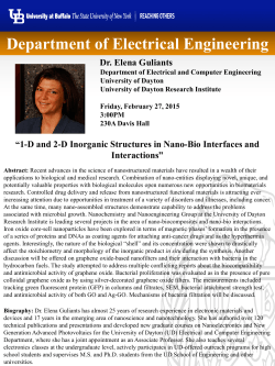


© Copyright 2026