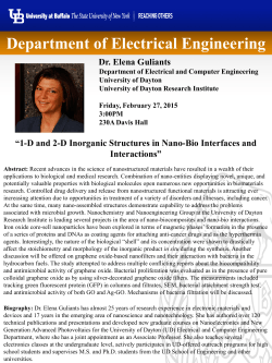
Departments of ECE and MSE, Cornell University
ECE 4070/MSE 5470: Physics of Semiconductor and Nanostructures
Spring 2015
Homework 9
Due on May 15, 2015 at 5:00 PM
Suggested Readings:
a) Lecture notes
Problem 9.1 (Electron velocity saturation at high fields in semiconductors)
At low electric fields, the velocity of electrons in a semiconductor increases linearly with the field
according to v ≈ µ F , where µ = eτ m / m * is the mobility and F is the electric field, with τ m being the
momentum scattering time. But when the electric field is cranked up, the electron velocity saturates,
because the electrons emit optical phonons each of energy !ω op every τ E seconds, dumping the energy
eFv they gain from the electric field every second. Setting up the equations for the conservation of
momentum and energy, and solving for the steady state yields an estimate of this saturation velocity.
!ω op τ m
⋅
. Show that for a typical
m*
τE
Show that the saturation velocity obtained by this scheme is vsat ≈
semiconductor for which !ω op ≈ 60 meV, m * ~ 0.2m0 , and τ m ~ τ E , the electron saturation velocity is of
the order of ~107 cm/s. This is a good rough number for the saturation velocity of most semiconductors.
Problem 9.2 (Electron Scattering and Mobility)
In this problem, we will explain the temperature
dependence of the electron mobility in some (not all!)
doped 3D semiconductors. The adjacent figure shows
the experimental result: at low temperatures, the electron
3
mobility goes as µ (T ) ~ T 2 , and at high temperature it
goes as µ (T ) ~ T
−
3
2
. We first connect the mobility to the
*
scattering times via the Drude-like result µ = e τ / m .
(a) Phonon scattering: We showed in class that the
scattering rate of electrons due to acoustic phonons in
semiconductors is given by Fermi’s golden rule result
for
time-dependent
oscillating
perturbations
1
2π
=
|< k' | W (r) | k >|2 δ (Ek − Ek' ± !ω q ) ,
τ (k → k') !
where the acoustic phonon dispersion for low energy (or
long wavelength) is ω q ~ vs q , and the scattering potential is W (r) = Dc∇ r ⋅ u(r) . Here Dc is the
deformation potential (units: eV), and u(r) = nu0 exp[iq ⋅ r] is the spatial part of the phonon displacement
1
wave, n is the unit vector in the direction of atomic vibration and q points in the direction of wave
propagation.
2 2
We also justified why the amplitude of vibration 2M ω q u0 ≈ N ph × !ω , where
N ph = 1 / [exp(!ω q / kBT ) − 1] is the Bose-number of phonons, and the mass of a unit cell of volume Ω is
M = ρΩ , where ρ is the mass density (units: kg.m-3). Show that a transverse acoustic (TA) phonon does
not scatter electrons, but longitudinal acoustic (LA) phonons do. Now show using your result of HW 8,
Problem 8.4 for the ensemble averaged τ that the electron mobility in three dimensions due to LA
phonon scattering is µ LA =
2 2π
3
e! 4 ρ vs2
( )
m*
5
2
3
~T
−
3
2
. This is a very useful result.
Dc2 (kBT ) 2
(b) Impurity scattering: Using Fermi’s golden rule, calculate the scattering rate for electrons due to a
screened Coulombic charged impurity potential V (r) = −
Ze2
r
exp[− ] , where Ze is the charge of the
4πε s r
LD
impurity, ε s is the dielectric constant of the semiconductor, and LD =
ε s k BT
is the Debye screening
ne2
length and n is the free carrier density. This is the scattering rate for just one impurity. Show using the
result in HW8, Problem 8.5 with a (1− cosθ ) angular factor for mobility that if the charged-impurity
density is
β=2
N D , the mobility for 3D carriers is
µI =
7
2
2 (4πε s ) (kBT )
3
2
π Z 2 e3 ( m
2
)
1
* 2
3
2
N D F[ β ]
3
2
~
T
.
ND
Here
β2
2m* (3kBT )
2
F[
β
]
=
ln[1+
β
]
−
L
is
a
dimensionless
parameter,
and
is a weakly varying
D
1+ β 2
!2
function. This famous result is named after Brooks and Herring who derived it first.
(c) Now combine your work from parts (a) and (b) of the problem to explain the experimental dependence
of mobility vs temperature and as a function of impurity density as seen in the Figure above.
Problem 9.3 (Interband optical absorption in graphene)
Graphene has two complete carrier pockets (or six 1/3rd carrier pockets) in the FBZ, as shown below.
2
E
Conduction
band
Valence
band
graphene
In each carrier pocket, the conduction and valence band dispersions are:
()
()
"
E c k = + ! v k = + ! v k x2 + k y2
"
Ev k = −! v k = −! v k x2 + k y2
where the wavevector is measured, for simplicity, from the pocket center (as opposed to from the zone
center) and the zero of energy is also chosen to coincide with E p . Assume that the temperature is close
to zero (i.e. T ≈ 0K) and the valence band is full and the conduction band is empty. Light of frequency ω
is incident normally on the graphene sheet, as shown below.
The average value of the momentum matrix element is:
!
2
m2 v 2
Pvc . nˆ
= o
2
Provided that the polarization unit vector of the incident field is in the plane of the graphene sheet.
Assume that the intensity of the incident light is I inc . Assume that for all practical purposes the photon
!
momentum is small enough to be taken as zero (i.e. q = 0 ).
a) Write an expression for the rate of stimulated absorption per unit area R ↑ (units: 1/m2-sec) in
graphene in terms of the incident light Intensity I inc . Make sure you include contributions from both
spins and both carrier pockets. Write your answer as an integral over k-space.
b) Evaluate your integral in part (a) and show that R ↑ can be written as:
⎧
µo
⎛I
⎞
⎪
R↑ = constant ηo ⎜ inc ⎟
⎨ ηo =
εo
⎪
⎝ !ω ⎠
⎩
Find the value of the “constant” in the expression above and also specify the units of this “constant”.
3
c) As the light crosses the graphene sheet, some photons are lost because of absorption in the graphene
sheet. From your knowledge of R ↑ and the incident light Inensity I inc find out what fraction of the
incident photon flux is absorbed in the graphene sheet. You will find, to your amazement perhaps, that
this fraction is independent of the light frequency as well as of any material parameter value and depends
only on few fundamental constants of physics. Find a numerical value for this fraction.
Problem 9.4 (Population inversion, optical gain, and lasing)
In class, we derived that the equilibrium optical absorption coefficient of a semiconductor is
2
⎛ e ⎞ 2π Pcv ⋅ nˆ
α 0 (!ω ) = ⎜ ⎟
ε 0 nω c
⎝ m0 ⎠
2
⋅ gJ (!ω − Eg ) , where gJ (!ω − Eg ) is the joint electron-photon DOS, and all
symbols have their usual meanings. We also found that under non-equilibrium conditions, the optical
absorption coefficient becomes α (!ω ) = α 0 (!ω )[ fv (k) − fc (k)] , where the electron occupation functions
of the bands are given by the Fermi-Dirac distribution fv (k) =
1
E (k) − Fv , but with a quasi-Fermi
1+ exp[ v
]
k BT
level Fv for the corresponding band as the mathematical means to capture non-equilibrium. Consider
semiconductors and heterostructures with parabolic bandstrcutures for the conduction and valence bands
Ev (k) = −
!2 k 2
!2 k 2
,
E
(k)
=
E
+
for this problem.
c
g
2mv*
2mc*
(a) Make a sketch of the equilibrium absorption coefficients α 0 (!ω ) for a bulk 3D semiconductor, and a
2D quantum well vs the photon energy !ω .
(b) Plot the Fermi difference function fv (k) − fc (k) as a function of the photon energy !ω for a few
choices of the quasi-Fermi levels Fv , Fc of the valence and conduction bands. Specifically, track the
photon energy at which the difference function changes sign from –ve to +ve.
(c) Now combine (a) and (b) to plot the non-equilibrium absorption coefficient α (!ω ) for the choices of
Fv , Fc from part (b). Discuss the significance of a negative absorption coefficient.
(d) Show that the requirement for population inversion is Fc − Fc > Ec − Ev = !ω . This is the famous
Bernard-Duraffourg condition for population inversion in semiconductor lasers.
(e) Based on your results above, explain why semiconductor heterostructure quantum wells have lower
injection thresholds for lasing than 3D bulk semiconductors. This idea and demonstration won Herb
Kroemer and Zhores Alferov the 2000 Nobel prize in physics.
Problem 9.5 (Superconductivity)
Briefly explain the basic idea behind the BCS theory of superconductivity, and why it was not possible to
obtain its microscopic theory from perturbative methods of quantum mechanics.
4