
Volume 17, No 4, 2014 - National Center for Transit Research
Volume 17, No. 4, 2014 Performance Measures for the Analysis of Rural Public Transit in Alabama Michael Anderson Tahmina Khan Sean J. Barbeau Kari Watkins Alan Borning OneBusAway Multi-Region – Rapidly Expanding Mobile Transit Apps to New Cities Friday Exception Scheduling in Transit Systems: An Exploratory Analysis When Data Are Limited Michael D. Benson Robert B. Noland Jeffrey M. Casello Geoffrey McD. Lewis Kevin Yeung Deborah Santiago-Rodríguez A Transit Technology Selection Model Subeh Chowdhury Avishai (Avi) Ceder Bruno Velty Measuring Public-Transport Network Connectivity Using Google Transit with Comparison across Cities Reid Ewing Allison Spain Effects of Light-Rail Transit on Traffic in a Travel Corridor Guang Tian J. P. Goates Todd Litman Gregory L. Newmark Nakin Suksawang Priyanka Alluri Albert Gan Katrina Meneses Fabian Cevallos Kirolos Haleem Dibakar Saha Omkarprasad S. Vaidya A New Transit Safety Narrative Conducting Visitor Travel Surveys: A Transit Agency Perspective Use of Movable Bus Stop Loading Pads: Feasibility and Design Alternatives Evaluating the Performance of Public Urban Transportation Systems in India N C T R Joel Volinski, Editor Lisa Ravenscroft, Assistant to the Editor EDITORIAL BOARD Robert B. Cervero, Ph.D. University of California, Berkeley William W. Millar American Public Transportation Association Chester E. Colby E & J Consulting Steven E. Polzin, Ph.D., P.E. University of South Florida Gordon Fielding, Ph.D. University of California, Irvine Lawrence Schulman LS Associates Jose A. Gómez-Ibáñez, Ph.D. Harvard University George Smerk, D.B.A. Indiana University Naomi W. Ledé, Ph.D. Vukan R. Vuchic, Ph.D., P.E. Texas Transportation Institute University of Pennsylvania The contents of this document reflect the views of the authors, who are responsible for the facts and the accuracy of the information presented herein. This document is disseminated under the sponsorship of the U.S. Department of Transportation, University Research Institute Program, in the interest of information exchange. The U.S. Government assumes no liability for the contents or use thereof. Volume 17, No. 4, 2014 ISSN 1077-291X The Journal of Public Transportation is published quarterly by National Center for Transit Research Center for Urban Transportation Research University of South Florida • College of Engineering 4202 East Fowler Avenue, CUT100 Tampa, Florida 33620-5375 Phone: (813) 974-3120 Fax: (813) 974-5168 Email: [email protected] Website: www.nctr.usf.edu/journal © 2014 Center for Urban Transportation Research Volume 17, No. 4, 2014 ISSN 1077-291X CONTENTS Performance Measures for the Analysis of Rural Public Transit in Alabama Michael Anderson, Tahmina Khan.................................................................................................... 1 OneBusAway Multi-Region – Rapidly Expanding Mobile Transit Apps to New Cities Sean J. Barbeau, Alan Borning, Kari Watkins.............................................................................14 Friday Exception Scheduling in Transit Systems: An Exploratory Analysis When Data Are Limited Michael D. Benson, Robert B. Noland.............................................................................................35 A Transit Technology Selection Model Jeffrey M. Casello, Geoffrey McD. Lewis, Kevin Yeung, Deborah Santiago-Rodríguez..............................................................................................................50 Measuring Public-Transport Network Connectivity Using Google Transit with Comparison across Cities Subeh Chowdhury, Avishai (Avi) Ceder, Bruno Velty..............................................................76 Effects of Light-Rail Transit on Traffic in a Travel Corridor Reid Ewing, Guang Tian, Allison Spain, J. P. Goates.................................................................93 A New Transit Safety Narrative Todd Litman............................................................................................................................................. 114 Conducting Visitor Travel Surveys: A Transit Agency Perspective Gregory L. Newmark............................................................................................................................ 136 Use of Movable Bus Stop Loading Pads: Feasibility and Design Alternatives Nakin Suksawang, Priyanka Alluri, Albert Gan, Katrina Meneses, Fabian Cevallos, Kirolos Haleem, Dibakar Saha.................................................................... 157 Evaluating the Performance of Public Urban Transportation Systems in India Omkarprasad S. Vaidya..................................................................................................................... 174 i Performance Measures for the Analysis of Rural Public Transit in Alabama Michael Anderson, Ph.D., P.E., and Tahmina Khan University of Alabama at Hunstville Abstract As rural public transit systems are vital to the livelihood of rural Americans, improving the operations of these systems is the focus of this work. The use of performance measures to evaluate operation is essential to maintain growth and avoid becoming stagnant. The main goal of this study was to examine existing performance measures (PM) and modify them to allow for comparison of performance among rural transit agencies in Alabama. The tasks presented in this paper are a review of performance measures, data collection, and data analysis for agencies in Alabama. The report concludes that performance measures can be developed that balance external factors in the analysis and allow for a fair comparison of agencies. Introduction Continually improving performance is necessary to avoid becoming stagnant or obsolete. Recently, the Transit Cooperative Research Program (TCRP) published Report 136, “Guidebook for Rural Demand-Response Transportation: Measuring, Assessing, and Improving Performance,” to serve as a typology for rural demand-response systems, identify factors that influence performance, and quantify performance improvements from specific actions. The low density in rural America, where only 17 percent of the nation’s population lives in 75 percent of the nation’s land area, makes the provision of transit particularly challenging (Carsey Institute 2006). The trend nationally is for the “aging” of the rural population, influenced by migration patterns away from rural America to urban America for younger people and the growth in the over-50 age group, both by total population and percent, in many rural locations (Ellis and McCollom 2009). In rural locations, access to health care and basic necessities is complicated by distance, terrain, and a population facing increased mobility challenges. This is where rural public transit systems fill mobility gaps. As rural public transit systems are vital to the livelihood of rural Americans, improving the operation of these systems is the focus of this project. The work was stimulated by the publication of TCRP Report 136, which provides guidance into performance measures Journal of Public Transportation, Vol. 17, No. 4, 20141 Performance Measures for the Analysis of Rural Public Transit in Alabama that were used to evaluate rural transit systems. Data to support the analysis presented in the guide were collected from the Alabama Department of Transportation and from specific agencies to determine the current levels of performance as the guide indicates. The measures presented in the guide were then modified to allow comparisons across rural transit agencies in Alabama. The main purpose of the study was to formulate a new methodology that eliminates the influences of uncontrollable factors, thus standardizing the performance measures defined in TCRP Report 136 to make a better comparison among different rural transit systems in Alabama. The objectives were to examine published performance measures and modify them to allow for comparison of performance among rural transit agencies in Alabama. The tasks presented in this report are a review of performance measures in the TCRP Report 136 and other sources, data collection, and data analysis for agencies in Alabama. The report concludes that performance measures can be developed that balance external factors in the analysis and allow for a fair comparison of agencies. Literature Review Literature related to defining the proper performance measures for rural transit that allow for comparison of different systems and the development of peer grouping methodology was reviewed and summarized. Performance Measures in Rural Transit A dissertation by Stephanedes (1979) on performance indicators and policy evaluation in rural transit proposed a list of 32 rural performance measures that reflect six specific conditions such as output, effectiveness, efficiency, cost-effectiveness, quality, and impact. Later, Radow and Winters (n.d.) stated four ways to measure rural transit performance: effectiveness, efficiency, quality, and impact, and described how rural transportation providers face unique challenges compared to urban transit systems, and how fixed route systems are different from demand responsive service. A paper by Kosky (2007) indicates selecting proper performance measures depends on data availability, reliability, and cost of collection, while noting that the key is simplicity and minimal overlapping. It presents eight key elements to measure system performance (both efficiency and effectiveness), including total expenses, variable expenses (i.e., fuel costs, maintenance, insurance, and employee salaries), vehicle hours, passengers, miles and number of vehicles, and a number of ways to look at the relationships between these numbers as particular ratios of key elements (Kosky 2007). As presented by Reilly et al. (1998), the main goal of rural demand responsive transportation (DRT) should be broken down to a small number of objectives based on data availability and data collection costs that are measured by clearly defined performance statistics so that the resource limitations of a system do not preclude an effective evaluation process. Reilly proposed a number of financial and non-financial indicators and describes how the performance evaluation process should be carried out (Reilly et al. 1998). TCRP Report 165, “Transit Capacity and Quality of Service Manual,” classifies demand responsive measures into two groups such as measures of availability (response time, service span, and service coverage) and measures of comfort and convenience (reliability, Journal of Public Transportation, Vol. 17, No. 4, 20142 Performance Measures for the Analysis of Rural Public Transit in Alabama travel time, and no-shows) (Kittelson & Associates et al. 2013). The performance of general DRT varies in terms of its productivity and depends on numerous factors such as size of the service area and its characteristics, locations of trip generators, and nature of trip demand that are quite similar to the factors mentioned in TCRP 136. Categories of Performance Measures in Urban Transit Upon investigating traditional transit performance measures in TCRP Report 88, “A Guidebook for Developing a Transit Performance-Measurement System,” 10 different categories of performance measures were summarized:, service delivery, community impacts, travel time, safety and security, maintenance and construction, economics, capacity, paratransit, and comfort (Cottrell and James 2009). One of the reviewed papers demonstrates how some Transit Performance Measures (TPMs) related to accessibility, mobility, and economic development recommended by the Performance-Based Planning Manual across all modes can be extracted from the bus dispatch system data (consisting of automatic vehicle location, communications, automatic passenger counters, and a central dispatch center) and can assist a transit agency in improving the quality and reliability of its service, leading to improvements for customers and operators alike (Bertini and El-Geneidy 2003). Performance Measures in Funding Allocation Formulas For allocating subsidies to rural public transit, Evans proposes an allocation formula applying equalization models that incorporate elements of cost (cost per trip or cost per mile), need (proportion of households in the service area), and performance (number of trips or passenger miles per unit of subsidy). A methodology in which funding was awarded based on population (proportional to population) and patronage (proportional to their subsidy per passenger trip) could be a practical way of allocating subsidies (Marshment 1998). To allocate funding, a performance index, PI, was developed that proposed the use of weighted performance rating that is a function of revenue/cost (R/C) ratio, annual trips per capita and new trips per capita (Sousa and Miller 2005). Karlaftis and Sinha’s paper (1997) evaluates whether subsidies have had differential performance impacts based on the type of operation and subsidy source. The five measures used in Karlaftis and Sinha’s study to capture the efficiency and effectiveness are revenue vehicle miles per employee, revenue vehicle miles per vehicle, revenue vehicle miles per operating expense, passengers per service area population, and passengers per vehicle. It concludes that subsidies from different sources (federal or state and local) have different effects on the performance of different types of paratransit systems (differentiated on the basis of whether they are publicly or privately operated) (Karlaftis and Sinha 1997). Peer Comparison Methodologies When comparing transit operation in various cities, an evaluation must consider the differences in urban form and land use, population, employment distribution, topography and climate, and structure variables accordingly to minimize these effects where variables must be disaggregated by areas of the metropolitan region that distinguish between transit service in the central city and in suburban areas. To identify variables for characterizing level of service into the three major components of quantity (the supply), quality (how good the service is), and cost/revenue (deals with economic factors though depends on Journal of Public Transportation, Vol. 17, No. 4, 20143 Performance Measures for the Analysis of Rural Public Transit in Alabama quantity and quality), Allen and Cesare (1976) concentrated on the checklist of about 45 attributes (referred to as characteristics or variables such as route density, passenger density, and operating ratio) plus the corresponding performance measures selected by a cooperative process (agreed upon by legislature, transportation agencies and the citizen’s groups that combines the operator’s experience, the state’s research and planning capabilities, the legislature’s policy making process, the local citizen’s needs and desires) that best reflects the mass transportation objectives of the community and contributes to transit level of service described as quality, quality, and cost/revenue (Allen and Cesare 1976). One of the earlier studies used z-scores of each system on each of the selected performance measures and a ranking scale developed by summing the selected indicator z-scores for each system called as ZSUM, to indicate the overall performance of a bus system (Fielding and Anderson 1983). Data Envelopment Analysis (DEA) methodology was used in earlier and recent studies to estimate relative scores in efficiency and effectiveness of various transit systems and compare individual systems to their peers in multiple performance measures (Arman, Labi and Sinha 2012; Ferronatto, Lindau and Fogliatto 2009; Fu, Yang and Casello 2007; Chu, Fielding and Lamar 1992). Principal Component Analysis (PCA) based indices take into account both efficiency and effectiveness leading to more reliable scores and perform better on data sets where variables are highly correlated (Ferronatto, Lindau and Fogliatto 2009). Ryus et al. (2011) focuses on the process used to identify peer-grouping factors, followed by determining groups of transit agencies that operate with similar external constraints and that provide similar types of service. Data were developed (or attempted to be developed) for each potential peer-grouping factor for each transit agency reporting to the National Transit Database (NTD). The factors were then evaluated based on variation between region or transit agencies, data availability, ease of maintenance, and existence of an alternative factor. Factors such as service area type, proximity, population density, percent low income, state capital, vehicle miles operated etc., are used to determine which potential peer agencies are most similar to the target agency. Individual likeness scores (the percentage difference between a potential peer’s value for the factor and the target agency’s value) determined for each individual screening and peer-grouping factor, can be used to calculate a total likeness score, where a score of 0 indicates a perfect match between two agencies (and is unlikely to ever occur) and a score of 10 means not at all alike (Ryus et al. 2011). Sum (screen factor scores) + Sum (peer grouping factor scores) Total likeness score = Count (peer grouping factors) To form a peer group, an agency would normally use the 8 or 10 agencies with the lowest total likeness scores and at least 4 peers are recommended at a minimum, to ensure an adequate basis for comparing performance results (Ryus et al. 2011). The Florida peer selection process attempts to identify comparable transit systems through a point scoring system with the following eight measures: (Gan, Ubaka, and Zhao 2002): Journal of Public Transportation, Vol. 17, No. 4, 20144 Performance Measures for the Analysis of Rural Public Transit in Alabama • Service area population density • Revenue miles • Average speed • Service area population • Vehicles operated in maximum service • Passenger trips • Revenue hours • Total operating expense The first three variables are considered primary, and the others are secondary. Under the scoring system, primary variables are given extra points. The performance of each of the potential non-Florida peers is compared with the average of the Florida systems for each of the eight measures. A peer receives one point for each measure for which it is within one standard deviation of the Florida system mean. One-half point is given for each measure that falls between one and two standard deviations from the Florida system mean. The scoring system can also be based on percentage rather than standard deviation. In the percentage-based method, a peer receives one point for each measure for which it was within 10 percent of the Florida system mean. One-half point is given for each measure that falls between 10–15 percent from the Florida system mean. In both cases, an extra one-half point is given for each of the three primary measures (Gan, Ubaka and Zhao 2002). Overall, there are many mechanisms to evaluate rural transit performance, which generally focus on a few main data elements and analysis trends. This study was to develop a simplified methodology that should reflect and comply with the guidance of TCRP Report 136, “Guidebook for Rural Demand-Response Transportation: Measuring, Assessing, and Improving Performance” (Ellis and McCollom 2009) and can be adapted easily by using readily available data. Data Collection This section discusses the data that were collected to perform the evaluation of the performance measures for Alabama’s rural transit systems. The data included information about the transit systems currently operating in Alabama and the counties they serve. The data of these agencies are required to be submitted to the Alabama Department of Transportation (ALDOT) on a quarterly basis and corresponding performance measures are used to track individual agency performance. Finally, the section presents other, non-controllable factors that might influence transit performance in the areas where the systems operate. These non-controllable factors are used later to compare system operation among providers. At the time of this report, there were 29 transit systems operating in 50 of Alabama’s 67 counties, with the majority being single-county operations. Each of the transit systems submits certain data/performance measures variables to ALDOT on a quarterly basis. Journal of Public Transportation, Vol. 17, No. 4, 20145 Performance Measures for the Analysis of Rural Public Transit in Alabama Using the data submitted by the agencies, a preliminary list of performance measures was established using guidance from the ALDOT and reviewed literature. The performance measures along with the variables are shown in Table 1. TABLE 1. Measures/Key Ratios Performance Measures (PM) Productivity (defined below) Passenger trips / vehicle hour Operating cost per vehicle hour (Operating + administrative cost) / vehicle hour Operating cost per vehicle mile (Operating + administrative cost) / vehicle mile Operating cost per passenger trip (Operating + administrative cost) / passenger trip Average passenger trip length Total passenger miles / total number of trips Average travel time Total passenger travel time / total number of passenger trips Hourly utilization Passenger hours / vehicles hours Mileage utilization Passenger miles / vehicle miles Operating cost recovery ratio Revenue / operating cost Equations Using Data / Performance Measures Variables It must be noted that the data from the quarterly reports submitted to ALDOT contained discrepancies that needed to be removed to obtain accurate performance measures. For example, vehicle miles (pull-out to pull-in, including deadhead miles and corresponding to accumulating vehicle hours, as per TCRP 136) were sometimes recorded as very large in comparison to passenger miles (sum of all passenger trip length that is measured from pickup to drop-off location, as per TCRP 136) and sometimes reported as less than passenger miles. Additionally, there were discrepancies in the revenue and cost values as charges were incurred in one quarter and the revenues were recorded in another. Problem Statement In reviewing the performance measures, there were some wide discrepancies across the transit agencies in the state. Table 2 shows the performance measures with average, best, and worst performance for the 29 agencies in Alabama. TABLE 2. Performance Measures Values (Average, High and Low), Alabama Transit Agencies Measures/Key Ratios Average Productivity (defined below) 2.81 7.14 0.90 Operating cost per vehicle hour 28.18 12.11 47.99 Operating cost per vehicle mile 1.93 0.97 3.85 Operating cost per passenger trip Best Worst 12.40 3.19 26.96 Average passenger trip length 5.36 1.73 16.46 Average travel time 1.75 0.11 42.27 Hourly utilization 2.16 42.47 0.10 Mileage utilization 0.81 1.07 0.46 Operating cost recovery ratio 0.63 1.58 0.15 These performance measures and results for the transit agencies in Alabama highlight the differences in operations throughout the state. For example, productivity (the measure of passenger trips per vehicle hour), which indicates how often the vehicles are carrying multiple passengers to similar destinations, ranges from 0.90–7.14. From an outsider’s Journal of Public Transportation, Vol. 17, No. 4, 20146 Performance Measures for the Analysis of Rural Public Transit in Alabama perspective, it could be concluded that agencies with higher than average productivity would use superior scheduling and dispatching skills as compared to agencies with lower productivity values. A similar statement could be made for all the performance measures; for example, the agencies with lower operating cost per passenger trip would be seen as superior to agencies with higher operating cost per passenger trip. However, when attempting to compare across agencies, there are several factors that need to be examined that are outside agency control. These variables were considered important, as they represented a normalization or equalization of the performance measures. For example, an agency in a very sparsely-populated area might have a lower productivity value simply due to the fact there are fewer people in the area to serve. Similarly, an agency might have a higher operating cost per passenger trip due to offering service in a larger county where trips might tend to be longer as locations are spaced out over a wider distance. These factors are outside the control of the operating agency and if these factors were taken into account, it might be possible to show that agencies with seemingly lower performance metrics are actually operating more efficiently than others with higher metrics simply based on population and service area size. These potential factors/non-controllable data, as per TCRP Report 136, can be measured using the following data such as: • Resident 2010 Census population • Number of residents in service area age 65 and older • Land area, square miles • Road length, miles • % road length miles >= 5% slope (as steep slopes create more wear on vehicles) • % road length miles >= 10% slope • % road length miles >= 15% slope • Mean slope % • Total number of rail crossing in the service area • Total number of intersections in the service area • Median household income, in dollars, 2010 • Shape factor to assess the shape of the service area to determine the ease of offering service The non-controllable data were further developed for use as performance measures, as shown in Table 3. Journal of Public Transportation, Vol. 17, No. 4, 20147 Performance Measures for the Analysis of Rural Public Transit in Alabama TABLE 3. Variable Data Needed Further Processing Type of Processing Older adult, age 65 and older Using access to determine the summation of age 65 and older Road length, miles Using ArcGIS summation % road length miles >= 5% Using ArcGIS slope raster from DEM. Contour of slope raster, summation of roadways intersect with >= 5% % road length miles >= 10% Using ArcGIS slope raster from DEM. Contour of slope raster, summation of roadways intersect with >= 10% % road length miles >= 15% Using ArcGIS slope raster from DEM. Contour of slope raster, summation of roadways intersect with >= 15% Mean slope % Using ArcGIS slope raster from DEM. Mean of slope raster Road and rail intersections Using ArcGIS, find number of roadways intersect with railways Intersections Exporting DBF from ArcGIS and opening table in Excel, count the instances where common FNODE and TNODE appear without duplicating same occurrence Shape factor (SF) Dissolving county boundaries by the boundary of transit system and calculating SF that is equal to {(perimeter/4)2 / (Area)} Data Analysis When examining the systems, it was determined that whereas most systems operate over a single county service area, there are others that are operating in sub-county areas or multiple counties: • Four locations operate in sub-county areas, either by serving only selected cities in the county or by serving only residents who live in the non-urban portion of a county. • Three agencies serve multiple counties. In an effort to remove bias from the results, a series of candidate systems was developed to test the effect of sub-county and multiple county results: • 22 systems exclude sub-county, urbanized, and multi-county systems • 26 systems exclude multicounty systems • 25 systems exclude sub-county and urbanized county systems The correlation and its P-values between factors and performance measures for the different sample sizes were determined. The P-value is the observed significance level of the test. If the observed significance level is less than the chosen significance level (alpha), then the researcher should reject the null hypothesis (no significant correlation) in favor of the alternative (a significant correlation). Otherwise, there is not enough evidence to reject the null hypothesis. Based on the results and to eliminate the differences in the extent and type of area covered by transit systems, it was decided to keep the sample size of 25 systems, eliminating the sub-county systems. Furthermore, it was determined that the values of correlation between factors and the variables of performance measures improve when 25 systems were analyzed rather than Journal of Public Transportation, Vol. 17, No. 4, 20148 Performance Measures for the Analysis of Rural Public Transit in Alabama total number of system in the state of 29, mentioned in the data collection section. The following factors were identified that are correlated with the variables of PM and describe most of other factors such as population, land area, intersections, and shape factor that are also correlated with PM variables : • Road length miles (RL miles) were correlated with all PM variables except passenger service hours and correlated with most of other factors (population, land area, intersections, and shape factor). • % road length miles >= 5% slope was correlated with operating and administrative costs and not explained by other selected factor. However, administrative cost does not include any maintenance cost and % road length miles >= 5% slope was not considered a correlated factor with administrative cost. The following factors were identified that are correlated with performance measures and describe most of other factors such as intersections and land area: • % of residents in the service area age 65 and older was correlated with mileage utilization and not explained by other selected factor. • RL miles were correlated with productivity and operating cost per passenger trip, and explains most other factors (land area and intersections). However, land area miles can explain the same number of other correlated factors. RL miles were selected because they show better correlation values with others. To remove the correlation of variable issue, several of the equations were modified. Most of the PM values were unchanged after incorporating the division because of the presence of the same factor in numerator and denominator. The division tool was applied for correlated factors with PM variables regardless of sign of correlation. Second, three of the performance measures correlated with the selected factors were divided by the corresponding factors to eliminate their influence from PM: productivity, operating cost per passenger trip, and mileage utilization. Finally, it can be seen that there are performance measures (presented in Table 1 on the right side as equations) related to operating cost that do not have any correlation with any factor, whereas as a PM variable, operating cost is correlated with % road length miles >= 5% slope. So, it was necessary to combine the findings of the above two analyses, namely correlated factors in PM variables and correlated factors for performance measures, and can be presented as one Table 4, where the bold rows are from PM results and others are from PM variables results. The only exception is for operating cost per passenger trip, which includes correlated factors both from PM variable and PM analyses. Journal of Public Transportation, Vol. 17, No. 4, 20149 Performance Measures for the Analysis of Rural Public Transit in Alabama TABLE 4. Equations after Incorporating Correlated Factors Results Original performance measures without incorporating any changes for correlation were given a ranking throughout the state based on best value. For example, if productivity or hourly utilization or mileage utilization or operational cost recovery ratio of any system had the highest value, that system was assigned as 1st rank. Performance measures related to operating cost, average time, or average length should have the lowest value assigned as 1st rank as the lower the operating cost or average time or length of a transit system, the better the system performs. After assigning the rank for each performance measure, the summation of ranks was again ranked to assess the overall performance of each system. Performance measures based on updated PM variables were ranked individually, and aggregated rankings were done similarly. Likewise, aggregated ranking of performance measures were calculated based on combined findings that considered the modified equations of Table 4. Examining the values for all agencies, essentially adding the ranking for the nine performance measures, creates a total statewide ranking. The following table (Table 5) shows Journal of Public Transportation, Vol. 17, No. 4, 201410 Performance Measures for the Analysis of Rural Public Transit in Alabama the rankings from the original performance measures and from using the equations presented in Table 4 (combined updated measure), along with the change. TABLE 5. Statewide Rank and Change Associated with Difference in PMs Agency Original Rank Modified Rank Change A 8 7 +1 B 24 14 +10 C 9 4 +5 D 6 23 -17 E 27 20 +7 F 7 3 +4 G 23 13 +10 H 19 11 +8 I 20 16 +4 J 29 28 +1 K 25 25 +0 L 11 12 -1 M 5 8 -3 N 16 21 -5 O 4 6 -2 P 12 17 -5 Q 10 10 +0 R 15 18 -3 S 28 29 -1 T 21 19 +2 U 22 22 +0 V 13 24 -11 W 2 2 +0 X 1 1 +0 Y 14 15 -1 Z 18 26 -8 AA 17 9 +8 BB 26 27 -1 CC 3 5 -2 Conclusions The main purpose of the study was to formulate a new methodology that eliminates the influences of uncontrollable factors, thus standardizing the performance measures defined in TCRP Report 136 to make a better comparison among different rural transit systems in Alabama. Existing measures were modified for comparison purposes in Alabama. After excluding correlated uncontrollable factors, it can be seen that the ranking of individual PM was changed. Sometimes, the lower rankings turn out to be the best Journal of Public Transportation, Vol. 17, No. 4, 201411 Performance Measures for the Analysis of Rural Public Transit in Alabama ranking after standardization. The aggregated ranking also shows significant difference for aggregated existing and updated ranking. It can be concluded that this methodology provides a useful way to standardize the performance measures by eliminating the effects of uncontrollable factors such as different terrain, population, and road coverage conditions etc., and rank those by maintaining a fair scale of judgment. The final recommendation is to use this tool to make a fair individual or aggregated ranking of performance measures among different rural transit systems. References Allen, William G., and Frank Di Cesare. 1976. Transit service evaluation: preliminary identification of variables characterizing level of service. Transportation Research Record, 606: 41-47. Arman, Mohammad, Samuel Labi, and Kumares C. Sinha. 2012. An assessment of the operational performance of public transit agencies using Data Envelopment Analysis (DEA) technique. Transportation Research Record, 2351: 30-37. Bertini, Robert L., and Ahmed El-Geneidy. 2003. Generating transit performance measures with archived data. Transportation Research Record, 1841: 109-119. Chu, Xuehao, Gordon J. Fielding, and Bruce W. Lamar. 1992. Measuring transit performance using Data Envelopment Analysis. Transportation Research Part A: Policy and Practice, 26: 223-229. Cottrell, Wayne D., and Bill James. 2009. Performance measures for personal rapid transit. Proceedings of the 88th Annual Meeting of the Transportation Research Board, Washington, D.C. Ellis, Elizabeth, and Brian McCollom. 2009. TCRP Report 136, Guidebook for Rural Demand Response Transportation: Measuring, Assessing, and Improving Performance. Washington DC: Transportation Research Board. Ferronatto, Luciana Guadalupe, Luis Antonio Lindau, and Flavio Sanson Fogliatto. 2009. Comparison of public transportation efficiency indices based on data envelopment analysis and principal component analysis. Proceedings of the 88th Annual Meeting of the Transportation Research Board, Washington, DC. Fielding, Gordon J., and Shirley C. Anderson. 1983. Public transit performance evaluation: Application to Section 15 Data. Transportation Research Record, 947: 1-7. Fu, Liping, Jingtao Yang, and Jeff Casello. 2007. Quantifying the technical efficiency of paratransit systems using the Data Envelopment Analysis method. Transportation Research Record, 2034: 115-122. Gan, Albert C., Ike Ubaka, and Fang Zhao. 2002. Integrated National Transit Database analysis system. Transportation Research Record, 1799: 78-88. Institute, Carsey. 2006. Demographic trends in rural and small town America. University of New Hampshire, Durham. Journal of Public Transportation, Vol. 17, No. 4, 201412 Performance Measures for the Analysis of Rural Public Transit in Alabama Karlaftis, Matthew G., and Kumares C. Sinha. 1997. Performance impacts of operating subsidies in the paratransit sector. Transportation Research Record, 1571: 75-80. Kittelson & Associates, Inc., Parsons Brinckerhoff, Inc. KFH Group, Texas A&M Transportation Institute, and Arup. TCRP Report 165: Transit Capacity and Quality of Service Manual. Washington, DC: Transportation Research Board, 2013. Kosky, Scott. 2007. Performance evaluation for rural transit systems. Rural Transit Assistance Program, Columbia, MO. Marshment, Richard S. 1998. Assessment of state procedures for allocating Section 5311 subsidies to rural public transit operators. Transportation Research Record, 1623: 63-67. Radow, Laurel J., and Chris Winters. 2011. Rural transit performance measurement. http:// www.ctaa.org/webmodules/webarticles/articlefiles/Rural_Transit_Performance_ Measurement.pdf (accessed November 21, 2011). Reilly, Jack, Edward Beimborn, and Robert Schmitt. 1998. Transit performance measurement. Adapted from NTI course “Improving Transit System Performance: Using Information Based Strategies,” developed at University of Wisconsin-Milwaukee, 1996-98. Albany, N.Y.. Ryus, Paul, et al. 2011. Development of the TCRP G-11 Transit agency peer-grouping methodology. Proceedings of the 90th Annual Meeting of the Transportation Research Board, Washington, DC. Sousa, Paul, and Eric J. Miller. 2005. Performance-driven transit funding model. Transportation Research Record, 1927: 73-81. Stephanedes, Y. J. 1979. Performance indicators and policy evaluation in rural transit. Ph.D. dissertation, Dartmouth College, Hanover, New Hampshire. About the Authors Dr. Michael Anderson ([email protected]) works as an Associate Professor in the Department of Civil and Environmental Engineering at the University of Alabama in Huntsville. His areas of interest include transportation planning/modeling, freight planning, traffic simulation, GIS application, traffic safety and development of decision support tools. Tahmina Khan ([email protected]) is a graduate student in the Civil and Environmental Engineering Department at the University of Alabama in Huntsville. Journal of Public Transportation, Vol. 17, No. 4, 201413 OneBusAway Multi-Region – Rapidly Expanding Mobile Transit Apps to New Cities Sean J. Barbeau, Ph.D. University of South Florida Alan Borning, Ph.D. University of Washington Kari Watkins, Ph.D. Georgia Institute of Technology Abstract Real-time transit information offers many benefits to transit riders, including reduced wait times and increased customer satisfaction. However, offering real-time transit services has been challenging for many transit agencies. While mobile applications (apps) have emerged as a preferred dissemination method for real-time information, it is typically cost-prohibitive for transit agencies to fund custom development of native mobile apps for all popular smartphone platforms. Third-party developers can offer services if an agency openly shares real-time data, but these individuals are volunteers whose priorities and deadlines may not be the same as the agency’s. As a result, few cities have full app portfolios that cover all smartphone platforms. This paper presents the OneBusAway multi-region project, a collaborative effort that is enabling the rapid expansion of native mobile transit apps to new cities. OneBusAway is an open-source transit information system that has provided real-time transit services to the Puget Sound (Washington) area since 2008. The new OneBusAway multi-region feature expands the coverage of the existing Android, iPhone, Windows Phone, and Windows 8 apps for OneBusAway to new cities, including Tampa and Atlanta. The multi-region system architecture, collaborative design and development process, and lessons learned from this ground-breaking project are discussed. The fundamental shift from proprietary to open-source software in the transit industry that has made this type of project possible also is examined. Introduction Real-time transit information has many benefits for transit riders. Past research has shown that transit riders who have access to real-time information perceive their wait time to be Journal of Public Transportation, Vol. 17, No. 4, 201414 OneBusAway Multi-Region – Rapidly Expanding Mobile Transit Apps to New Cities around 30 percent shorter than riders who do not have access to real-time information (Watkins et al. 2011). Additionally, real-time information users save almost two minutes in actual wait time, which has a very high disutility value and can be used to perform other tasks. Four Federal Transit Administration (FTA) workshops, held in Seattle (Washington), Salt Lake City (Utah), Columbus (Ohio), and Providence/Kingston (Rhode Island), concluded that real-time information attracts new riders who are otherwise reluctant to start using transit (Cluett et al. 2003). Similarly, a study in Chicago found modest ridership gains from real-time information even prior to wide usage of smart phones (Tang and Thakuriah 2012). Interviews with transit riders in San Francisco and Seattle in 2010 revealed that when the real-time information system was down, some riders elected not to ride the bus (Steinfeld and Zimmerman 2010). Riders also can use the information to adjust their own use of the transit system, e.g., by taking a different less-crowded bus, which can benefit other riders as well (Zimmerman et al. 2011). Other benefits identified in surveys include increased walking (i.e., public health benefits) and, for some riders, increased feelings of safety while waiting, particularly at night (Ferris et al. 2010; Gooze et al. 2013). With the number of smartphone users among transit riders being similar to those in the general population, providing app-based real-time information could be a major benefit to a large proportion of riders (Windmiller et al. 2014). However, offering real-time information services to transit riders has significant challenges. The cost for a transit agency to implement both Automatic Vehicle Location (AVL) technologies and information dissemination technologies (e.g., electronic signs, mobile phone apps) is not trivial, ranging from approximately $800,000 for a 17-vehicle fleet to $24 million for a 1,900-vehicle fleet (Parker 2008), especially in the public sector where budgets are under pressure. This estimate does not include the cost of mobile apps, which also is significant. The development cost for a business app that includes real-time information can be upwards of $150,000 (Lauvray 2011); understandably, agencies have cited development costs as being the primary barrier for offering “official” transit agency mobile apps (Wong et al. 2013). Another issue is the multiplicity of smartphone platforms. Agencies are reluctant to support all major platforms due to costs, yet choosing which one or two platforms to support also can be difficult. Since riders have shown a preference for accessing real-time information via mobile apps (versus other methods such as text-messages or websites [Watkins et al. 2011]), agencies must find another cost-effective solution for providing mobile apps to riders. One strategy for increasing the number of mobile transit apps at a transit agency is for the agency to share static (i.e., schedule) and real-time transit information with the general public as “open data”(Barbeau 2013; Wong et al. 2013). Third-party developers (individuals not associated with the transit agency) can then independently develop and release mobile apps to the general public. This strategy has successfully produced a number of third-party transit apps at several agencies in the U.S., including Bay Area Regional Transit (BART) in San Francisco (San Francisco Bay Area Rapid Transit District 2012), TriMet in Portland (TriMet 2012), Metropolitan Transportation Authority (MTA) in New York (Authority 2012), and Massachusetts Bay Transportation Authority (MBTA) (Massashusetts Bay Transportation Authority 2012). However, these independent developers may not have the same priorities and deadlines as agencies. For example, if a developer does Journal of Public Transportation, Vol. 17, No. 4, 201415 OneBusAway Multi-Region – Rapidly Expanding Mobile Transit Apps to New Cities not fill the need for an app on a particular platform or an app with particular features (e.g., an accessible interface for individuals with visual or other disabilities), then no such app will exist. Additionally, not all cities in the U.S. have robust high-tech transit populations and developer communities. In these cities, app growth is more modest (Hillsborough Area Regional Transit 2012). And, since real-time transit data formats often differ between cities, apps for one city cannot be shared easily with another. OneBusAway, a real-time transit information system originally created by researchers at the University of Washington (UW) (Figure 1), takes a new approach to the problem of transit information dissemination (University of Washington 2012). FIGURE 1. Homepage of open-source transit information system OneBusAway in Puget Sound Unlike traditional transit industry software, OneBusAway is open-source, meaning that the source code for the software is openly available for anyone to download, configure, alter, and deploy (OneBusAway Organization 2013). In addition to being open-source, OneBusAway supports popular bulk transit data formats such as General Transit Feed Specification (GTFS) (Google 2012), GTFS-realtime (Google 2012), and Service Interface for Real Time Information (SIRI) ((CEN) 2012), which means that anyone with access to transit data in these formats can launch his/her own OneBusAway service for his/her city. Furthermore, OneBusAway includes open-source native mobile apps for iPhone, Android, Windows Phone, and Windows 8, which provide rich functionality and responsiveness beyond that typically available in web applications. OneBusAway has been used to jump Journal of Public Transportation, Vol. 17, No. 4, 201416 OneBusAway Multi-Region – Rapidly Expanding Mobile Transit Apps to New Cities start several pilot and production deployments of real-time transit information systems (OneBusAway 2012). It also has served as the foundation of several research projects that aim to better understand how real-time information impacts transit riders (Ferris 2010; Ferris et al. 2010; Watkins 2011; Watkins et al. 2011; Gooze et al. 2013; Brakewood 2014). However, until recently, there was a key limitation with the original OneBusAway project—the OneBusAway mobile apps in the respective app stores (i.e., Google Play, Apple App Store, Windows Phone Store, Windows Store) were configured to work only in Puget Sound, where OneBusAway originally was developed. Extending the reach of the OneBusAway apps for iPhone, Android, Windows Phone, and Windows 8 to new cities raised many questions: • Should researchers or transit agencies launching new installations of OneBusAway in other regions also launch their own versions of each app in that region? • If these researchers or transit agencies wanted to make use of project-wide OneBusAway apps, how could these apps be configured to work in new OneBusAway cities? • Should OneBusAway app users be required to manually configure their apps to work in the correct city? Or, if a centralized server directory was provided, who would be responsible for implementing and supporting this directory? And who would make the required changes to the apps to use the directory? • Would third-party developers be willing to support new versions of their apps in new cities? • How should user feedback in multiple cities be directed to the right person (i.e., app developer or regional OneBusAway server administrator)? This paper presents the OneBusAway multi-region project (OneBusAway 2013), which investigated these questions with the goal of producing a sustainable, low-maintenance, cost-effective system that would support the rapid expansion of mobile transit apps for iPhone, Android, Windows Phone, and Windows 8 to new cities around the world. Background There are two primary developments in the transit industry over the last decade that made the OneBusAway multi-region project possible: the development of the original OneBusAway open-source project and the emergence of open transit data. OneBusAway started as a student project at UW in Seattle, motivated by the simple desire to have a truly usable interface for real-time transit information. It evolved into the PhD dissertation work of Brian Ferris (Ferris 2011) and Kari Watkins (Watkins 2011) and, at the same time, it spread virally to serve 50,000 unique weekly transit riders without official support from the transit agencies and with little outreach or publicity. Sound Transit, King County Metro, and Pierce Transit provided financial support for UW to continue operating OneBusAway from summer 2011 until summer 2013, at which point it was transitioned to Sound Transit. Journal of Public Transportation, Vol. 17, No. 4, 201417 OneBusAway Multi-Region – Rapidly Expanding Mobile Transit Apps to New Cities The second factor that makes OneBusAway multi-regionally feasible is the growing availability of open transit data and, in particular, the emergence of several de-facto transit data standards such as GTFS (Google 2012). As of December 2012, more than 500 agencies worldwide are sharing static (i.e., schedule) data in the GTFS format (Front Seat Management 2012), which allows third-party developers to create transit apps based on these data. GTFS was originally created by Google and TriMet in 2005 as a lightweight and easily-maintainable transit data format for the Google Transit trip planner (Roth 2012). While many agencies originally provided GTFS data for Google Transit, many transit and multimodal applications based on GTFS data have emerged (Barbeau and Antrim 2013), including OneBusAway. In addition to static data, OneBusAway also requires a real-time data source. Real-time transit data formats can be categorized into two magnitudes: fire-hose and faucet (Barbeau 2013). Fire-hose data formats contain a complete set of the entire state of the transit system, including all known estimated arrival times and all real-time vehicle locations for all routes and stops. In contrast, faucet data formats contain a precise subset of transit data, typically in response to a specific query (e.g., “The next bus on Route 16 will arrive at stop ID 100 in 5 minutes.”). GTFS-realtime and SIRI have emerged as the two most popular fire hose open data formats (Barbeau 2013). The OneBusAway server software can import both GTFS-realtime and SIRI data frequently (e.g., every 30 seconds) to reflect real-time changes for the entire transit system. Other proprietary formats such as OrbCAD FTP and Nextbus also are supported. And since OneBusAway is open-source, support for new formats can be added by any developer (OneBusAway 2012). As a result, the OneBusAway server software can be deployed with few modifications in any city that provides data in the above formats. One of the primary functions of the OneBusAway server is to take fire-hose data as input and provide faucet data as output, on demand, to thousands of apps. OneBusAway currently supports a custom-designed Representational State Transfer (REST) Application Programming Interface (API) for the faucet data, which allows the iPhone, Android, Windows Phone, and Windows 8 apps to retrieve real-time transit data specific to a device’s location and/or user’s request (OneBusAway Organization 2013). Comparison to Other Real-Time Transit Applications The open-source nature of OneBusAway is a key differentiator from commercially-available apps such as Moovit, Google Maps, Apple Maps, Microsoft Bing, Embark, RouteShout, Nokia Here, The Transit App, Citymapper, and Tiramisu. These “closedsource” applications all are operated by a single entity that has full control over what cities are supported. A city can request to be included, but it may not be added to the service. Business decisions, such as Apple’s choice to remove Google Maps in mid-2012, resulting in the loss of transit directions for iPhone users, also can instantly leave riders without any transit information. OneBusAway provides a different model—the software source-code is openly provided to the general public. Therefore, each region can independently create and operate its Journal of Public Transportation, Vol. 17, No. 4, 201418 OneBusAway Multi-Region – Rapidly Expanding Mobile Transit Apps to New Cities own OneBusAway server, and one region’s actions have no effect on another. Additionally, if a OneBusAway regional operator shuts down, another operator in the same region can resume the service. While there are significant advantages to the independent nature of OneBusAway regions, this independent design also creates the need for some initial coordination when determining how the OneBusAway mobile apps will interact with these independently-operated servers. A solution—the OneBusAway multi-region architecture—is discussed in the following section. This solution can be described as a “you bring the server, we bring the apps” approach, where the OneBusAway apps are centrally maintained and available to all regions, but each regional server is independently created and operated. This architecture, enabled by the open-source nature of the project, is unique to OneBusAway. Additionally, OneBusAway provides native mobile apps on four different platforms (Android, iPhone, Windows Phone, and Windows 8), which is more than any of the previously-mentioned commercially-available solutions. Multi-Region Architecture Design Decisions There were several possible strategies for making the OneBusAway mobile apps available in other cities beyond Puget Sound, one of which was to mirror the replication process of OneBusAway servers for new cities. When a new city wants to set up a new OneBusAway server, engineers would copy the OneBusAway server source code, configure it to access the new city’s real-time transit data, and deploy the copy to a server in the new city. This new OneBusAway server would then provide real-time information via a website. To mirror this strategy for the mobile apps, engineers in the new city would copy the source code for the iPhone, Android, Windows Phone, and Windows 8 apps. Then, the source code for the apps would be changed to use the local OneBusAway server (instead of the Puget Sound server), as shown in Figure 2. Finally, these modified apps would be deployed to the respective app markets with names such as “OneBusAway Tampa” or “OneBusAway Atlanta.” This strategy has the advantage of each city acting independently to deploy mobile apps without requiring any coordination among cities. However, this approach has three major drawbacks: 1. Sustainability – Each city would need to find new developers to maintain and update the local Android, iPhone, Windows Phone, and Windows 8 apps. This is clearly undesirable, as it is already challenging for many cities to find developers interested in developing transit apps. 2. Fragmentation – There would be one copy of each mobile app source code for each city. Therefore, for every bug fix in each mobile app, developers in each city would all have to adapt that fix to their particular modified version of the app. This creates source code that is difficult to maintain, limiting shared app improvements among cities. Additionally, when users try to download the app from the respective app store, they would be presented with a list of OneBusAway apps from all cities to Journal of Public Transportation, Vol. 17, No. 4, 201419 OneBusAway Multi-Region – Rapidly Expanding Mobile Transit Apps to New Cities choose from (e.g., “OneBusAway Tampa,” “OneBusAway Atlanta”), which places the burden on the user to find and install the correct app. 3. Scalability – The above two problems increase in complexity as OneBusAway is scaled up to include more and more cities. FIGURE 2. Possible design for OneBusAway with duplicated mobile apps for each city An alternate approach is for a group of pilot cities to work together and create a coordinated OneBusAway multi-region system (Figure 3). Here, a centralized OneBusAway directory is created with a list of known OneBusAway servers in various cities. Then, the existing iPhone, Android, Windows Phone, and Windows 8 apps are modified so they discover available OneBusAway servers from the directory (i.e., “Regions API”), as shown in Figure 3a. The app compares the user’s real-time location to the list of server locations (Figure 3b) and then connects to the closest server to retrieve route, stop, and arrival information (Figure 3c). FIGURE 3. Current OneBusAway multiregion architecture Journal of Public Transportation, Vol. 17, No. 4, 201420 OneBusAway Multi-Region – Rapidly Expanding Mobile Transit Apps to New Cities Using this approach, the complexity of the OneBusAway multi-region system is hidden from the user, and users in all cities download the same app from the mobile app stores. Additionally, only a single copy of the source code for each app needs to be maintained, and users in all cities would immediately benefit from app improvements. This strategy requires more work and coordination up front for the pilot cities, including the original third-party app developers. However, it drastically reduces sustainability and fragmentation problems for the future of the project, making the system scalable and reducing the overhead of adding more cities to the project. The overall OneBusAway project also benefits from this coordination through additional contributions and feedback from users and developers in multiple cities. Therefore, this strategy was chosen for the OneBusAway multi-region project. Detailed Protocol Figure 4 shows the detailed protocol used in the multi-region architecture, including interaction with both the Regions API and a regional OneBusAway server. When the user first installs and starts the app, the app retrieves a list of region information from the project-wide Regions API and saves this list on the mobile device. Then, the device compares the real-time location of the user to the list of region locations and automatically selects the closest region to the user. If there are any problems with device positioning, the user also can be presented with a list of available OneBusAway regions to choose from. After the region has been selected, the app directly contacts the regional OneBusAway server to retrieve information about stops and routes that can then be shown to the user. For example, the app might show a set of nearby bus stops on a map. The user can then select a stop to see estimated arrival times for that location. The app then contacts the regional OneBusAway server again to get a list of estimated arrival times for the given stop ID and show this information to the user. At this point, the user may close the app. The next time the user starts the app, it compares the user’s real-time location to the list of regions stored on the device (i.e., the most recently cached list from the Regions API) in the background to avoid interrupting the user experience. If the user is still in the same region, it continues using the previously-identified server. In the less likely event that the user has moved into a different OneBusAway region (e.g., traveled between cities) since last app startup, the app will automatically switch to the currently closest OneBusAway region, fetch information from that regional server, and move the map to the user’s new location. The implementation of different OneBusAway servers covering different geographic areas is thus completely transparent to the user. Occasionally, there will be changes to the list of servers and configuration information, including the addition of new regions. Since this information is not expected to change frequently, the mobile app only occasionally refreshes the local copy of region information from the Regions API—once per week in the current design. (This timeframe was selected to balance a reasonable refresh rate to detect new regions against adding additional communication between the mobile device and server, which has an impact on mobile device battery life and increases server load. So far, this timeframe has worked well Journal of Public Transportation, Vol. 17, No. 4, 201421 OneBusAway Multi-Region – Rapidly Expanding Mobile Transit Apps to New Cities in practice.) Thus, the mobile app operates mostly independently of the Regions API. This design also allows the system to scale easily, since as each new OneBusAway city is added, the vast majority of the new traffic will be handled by the regional OneBusAway server in that area, with only a small increase in traffic for the centralized Regions API. FIGURE 4. Protocol used by mobile apps to connect to a regional OneBusAway server Journal of Public Transportation, Vol. 17, No. 4, 201422 OneBusAway Multi-Region – Rapidly Expanding Mobile Transit Apps to New Cities Mobile App Modifications For the multi-region project to be successful, two issues needed to be addressed for each of the iPhone, Android, Windows Phone, and Windows 8 apps: 1. A developer with skills specific to that mobile app platform would need to modify the app to support the multi-region architecture. 2. The third-party developers who publish each of the four OneBusAway apps to respective app stores (e.g., Google Play, Apple App Store, Windows Phone Store, Windows Store) would need to agree to publish a new multi-region version of their mobile apps. Since the apps are open-source, Issue #1 could be resolved by another developer, not necessarily the primary maintainer of the mobile app. A detailed discussion of the advantages of this open-source model, as well as various collaboration tools that facilitate this process, can be found in the “Collaborative Process” section of this paper. Issue #2 is not difficult to achieve if the third-party developers are actively maintaining their apps and communicating with others participating in the OneBusAway community. If the developer of the app has the development environment set up and another contributor has made the source code modifications, it would take a few hours of effort to review the changes, compile a new release, and publish this new version to the respective app store. An important aspect of Issue #2 is the potential for a significant increase in user questions and feedback when the app is launched in a new city. For example, as of July 25, 2013, the OneBusAway Android app was actively installed on 141,817 devices, with a total of 234,281 downloads primarily for just the Puget Sound area. To avoid overwhelming the mobile app developers with a large amount of user feedback for new cities, the decision was made to have the “Contact Us” button in all the apps report information to the regional OneBusAway administrator. This design scales well as new OneBusAway administrators and support teams for each new OneBusAway region are added. Further, the current OneBusAway app developers and OneBusAway server administrators indicate that the vast majority of user feedback pertains to issues specific to the region (e.g., errors in the schedule and real-time data), not to the mobile app. It also is often not clear to users where the source of the problem lies, and troubleshooting sometimes requires knowledge of the system operation. Therefore, the OneBusAway administrators handle the majority of feedback and direct any application-specific feedback to the respective application developers as needed. Overall, as discussed later, the OneBusAway mobile app developers were generally enthusiastic participants in this project, since it immediately made their work more widely available to a much larger number of users. OneBusAway Server Administrators For the mobile apps to have up-to-date information for each region, OneBusAway regional server administrators must have a way to update a centralized OneBusAway Server Directory. This process must be low effort to implement and maintain, both for the central server directory administrator and the individual regional OneBusAway server administrators. Journal of Public Transportation, Vol. 17, No. 4, 201423 OneBusAway Multi-Region – Rapidly Expanding Mobile Transit Apps to New Cities A Google Doc spreadsheet was selected as the primary data entry tool for regional OneBusAway server administrators. Google Docs provides a reliable, ready-to-use platform for data entry into a spreadsheet that includes access control and data output in the Comma-Separated Values (CSV) file format. The Google Doc is configured to alert a set of administrators that oversee the entire OneBusAway open-source project, referred to as “Multi-region Administrators,” upon any edits. The multi-region administrator runs a Python script to convert the CSV output of the Google Doc to regions.json and regions. xml files, which are then made available to mobile devices via a web server as the Regions API. Thus, adding a new region to the Regions API is fairly simple. OneBusAway Regions As of August 2013 (just prior to the launch of the multi-region project), the OneBusAway software suite was deployed to Puget Sound, Tampa, and Atlanta. MTA in New York uses a modified version of OneBusAway for the MTA Bus Time project (Metropolitan Transportation Authority 2012). Detroit has used the OneBusAway software to implement its “Text-My-Bus” text-messaging service for transit riders (Code for America 2012). In Puget Sound, real-time data from several regional transit agencies (King County Metro, Sound Transit, Pierce Transit, and Intercity Transit) is provided to a single OneBusAway instance hosted by Sound Transit. King County Metro’s data are provided by a dedicated HTTP server that is made available to OneBusAway, Pierce Transit are provided via FTP from a secure file server, Intercity Transit are provided via HTTP, and Sound Transit data are provided via other agencies that operate the Sound Transit vehicles under contract. The system also has schedule-only data from a number of other agencies, including Community Transit, Washington State Ferries, the City of Seattle, and the Seattle Children’s Hospital Shuttle. Additional real-time data feeds are expected in the future. In Tampa, the University of South Florida (USF) team created an open-source GTFS-realtime feed for Hillsborough Area Regional Transit (HART)’s OrbCAD AVL SQL Server database (University of South Florida 2013) and used the GTFS-realtime feed as input to the OneBusAway Tampa server. In Atlanta, the Georgia Tech team created a GTFS-realtime feed from the Metropolitan Atlanta Rapid Transit Authority (MARTA) proprietary REST API real-time bus data feed and used this as input to the OneBusAway Atlanta server. The effort required to create a new OneBusAway server deployment and participate in the OneBusAway multi-region project is moderate. An agency or researcher must: 1. Obtain access to static transit schedule data in GTFS format and to a real-time transit data source. 2. Install and configure a OneBusAway server. 3. Contact the OneBusAway group to include the new region in the central directory. Collaborative Process Creating the process and infrastructure to rapidly expand mobile transit apps to new cities required a large collaborative effort. As mentioned earlier, individual OneBusAway server administrators were involved in the multi-region architecture design to ensure that the process to add and maintain servers was not effort-prohibitive. App developers were Journal of Public Transportation, Vol. 17, No. 4, 201424 OneBusAway Multi-Region – Rapidly Expanding Mobile Transit Apps to New Cities an integral part of the design process for the implementation and maintenance of the Regions API. The official formation of OneBusAway Board of Directors in January 2013 helped solidify the general OneBusAway project governance model, and members of the board served as key champions in Puget Sound, Atlanta, and Tampa to lead the multi-region process and coordinate the involved parties. Since participants were geographically dispersed, modern technology played a large role in communication and coordination. The OneBusAway Developers Google Group (OneBusAway 2013) served as the primary group email list. The OneBusAway Board of Directors also held scheduled monthly phone calls for progress updates. Considering that the OneBusAway multi-region project involved a substantial software engineering effort, the most important enabler of the project was the open-source ecosystem surrounding OneBusAway. Recently, open-source projects such as OpenTripPlanner (OpenPlans 2012), a multimodal web-based trip planning solution, and OneBusAway have emerged as open-source alternative to proprietary vendor-based solutions. Opensource transit projects provide the opportunity for agencies to invest in a common set of tools for a common set of needs—in this case, trip planning and real-time customer information systems. OneBusAway has flourished as an open-source system. Key tools enabling software development collaboration surrounding OneBusAway are the Git version control system (Software Freedom Conservancy 2013) and Github.com, an online software project hosting site that uses Git for version control. Git is a fully-distributed version control system that allows multiple developers to independently work on a project and then easily merge their contributions back into a single project. Github hosts projects versioned with Git and allows developers to communicate easily via email and the website to discuss issues for fixing bugs or implementing new features. The OneBusAway Github organizational account currently features 39 individual projects, or “code repositories,” and 15 official members are under this account. Among the open-source projects are the main OneBusAway server software and apps for Android, iPhone, Windows Phone, and Windows 8, as well as various tools to produce and transform transit data. An important benefit of Github is the ability of any Github user to easily “fork” (create a copy of) any OneBusAway project. These users can then edit and modify the copy to meet their own needs. Major copies of the main OneBusAway server project include the modifications specific to OneBusAway Tampa, OneBusAway Atlanta, MTA Bus Time, and Detroit’s TextMyBus. Forking a project on Github also provides the ability to merge improvements back into the main project from any copies via “pull requests.” In other words, a developer can create a copy of the project with little coordination with the original developer, learn about the project on their own timeline, implement a new feature or bug fix, and then submit this improvement back to the original project owner for review and possible inclusion in the main application. The Git version control system makes merging these contributions fairly straightforward. The OneBusAway multi-region project benefited heavily from contributions by developers who were not the original authors of the respective OneBusAway apps, indicating that this project would not have been successful in a traditional closed-source software Journal of Public Transportation, Vol. 17, No. 4, 201425 OneBusAway Multi-Region – Rapidly Expanding Mobile Transit Apps to New Cities environment where the only contributors are the official project owners. For example, the Android multi-region feature was started by the original author in Seattle, but was completed by a contributor from Tampa who was interested in accelerating the availability of the app in Tampa. The iPhone app had the most contributors (4 in Puget Sound and 1 in Atlanta) to bring the multi-region feature to full working order. Numerous developers and tech-savvy users from Puget Sound, Tampa, and Atlanta also helped in testing early versions of the applications. Both the Windows 8 and Windows Phone multi-region updates were completed entirely by the author of the Windows 8 app. To keep the source code uniform in format and structure, the various OneBusAway projects (e.g., server code, mobile apps) have style guides that can be used by software development tools to re-format any new code to match the project. Additionally, to ensure that the source code remains freely available under a common open-source license, third-party developers are required to sign an Individual Contributor License Agreement (ICLA) that specifies that copyright and patent rights for their contribution are assigned to the project. Results In the first half of 2013, the four OneBusAway native mobile applications were modified by mobile app developers to interact with the Regions API as part of the multi-region architecture. In August 2013, the multi-region apps were published on each of the respective app stores and made available in both Atlanta and Tampa, with no perceptible difference to users in Puget Sound. As a result, transit riders in Tampa and Atlanta had access to real-time transit information via Android, iPhone, Windows Phone, and Windows 8 apps. To the knowledge of the authors, the simultaneous launch of real-time transit apps on four native app platforms in more than one city is unprecedented in the transit industry. There was substantial growth in the use of OneBusAway in the year following the multi-region launch. In August 2013, the OneBusAway Android app was actively installed on 141,817 devices, with a total of 234,281 downloads for the Puget Sound area. One year later, in August 2014, after launching in Tampa, Atlanta, Washington, DC (beta), York (Canada) (beta), and Bear Transit for the University of California, Berkeley (beta), there were 219,460 active installs with a total of 336,681 downloads. In other words, over the course of one year, more than 77,000 active Android devices were added to the system (approximately 54% increase). iOS users grew by approximately 20 percent (approximately 117,000–140,400) over the same time period. Windows Phone app downloads grew from 41,950 to 60,751, a growth of approximately 44 percent. Windows 8 app use increased by around 3,000 downloads. Studies of the effectiveness of OneBusAway regarding the user experience and impacts on transit riders have been reported in multiple papers (Watkins et al. 2011) (Ferris et al. 2010; Ferris 2011; Watkins 2011), including issues with accuracy and rider perception (Gooze et al. 2013). Although these studies took place in Seattle, additional work is being undertaken in Tampa, New York, and Atlanta (Brakewood 2014) (Brakewood et al. 2014). In short, OneBusAway provides an enhanced user experience, especially in regards to the experience of waiting for the bus to arrive. Journal of Public Transportation, Vol. 17, No. 4, 201426 OneBusAway Multi-Region – Rapidly Expanding Mobile Transit Apps to New Cities OneBusAway has proven to be a reliable platform for delivering transit agency data. From August 2013 to August 2014 in Tampa, the only interruptions in service of OneBusAway to customers were related to internal HART networking issues, not problems with the OneBusAway software or hardware infrastructure. To avoid future issues caused by internal network infrastructure, HART moved hosting OneBusAway to a cloud computing service. Since this time, there have been no further interruptions of OneBusAway service to users. As a result, both agencies and riders have generally been pleased with the deployment of OneBusAway. HART Interim Chief Executive Officer Katharine Eagan stated, “We’re excited with how our customers in Tampa have been so quick to use the OneBusAway app. It has truly enhanced the rider’s experience because they have the answers they need right at their fingertips, and it demonstrates that our patrons appreciate our efforts to bring them innovative solutions.” The most significant long-term result of the OneBusAway multi-region project is the ease of future expansion of the OneBusAway apps to new cities; adding a new city is as simple as that city setting up a new OneBusAway server and adding that server information to the OneBusAway Server Directory. Other long-term benefits include an increased incentive for developers in the new cities (e.g., Tampa, Atlanta) to contribute to the OneBusAway project, as new features will now be visible in their own cities, resulting in a larger OneBusAway developer community that will continue to grow as new cities are added. A larger development community also reduces the burden on a single entity (e.g., UW) to support the OneBusAway project and, instead, spreads out demands for paid staff and volunteers among multiple agencies and universities. New apps continue to emerge as part of this community; in April 2014, a beta version of OneBusAway for Google Glass was created and is available in all OneBusAway regions. In conjunction with the multi-region app launch, the home page for the OneBusAway project at http://onebusaway.org was converted from being specific to Puget Sound to encompassing all cities involved in the project (Figure 5). FIGURE 5. New OneBusAway multiregion website showing multiple cities with shared OneBusAway mobile apps Journal of Public Transportation, Vol. 17, No. 4, 201427 OneBusAway Multi-Region – Rapidly Expanding Mobile Transit Apps to New Cities This allows riders to conveniently access regional OneBusAway services. Information for transit agencies interested in their own OneBusAway deployments, developers who want to contribute to the project, and researchers interested in academic publications related to OneBusAway also are included. A straightforward naming scheme for region URLs (e.g., http://tampa.onebusaway.org, http://pugetsound.onebusaway.org) makes it easy to add new regions while at the same time maintaining the identity of the project as a whole. Lessons Learned As is the case with many pioneering efforts, the OneBusAway multi-region project yielded many lessons learned. As discussed earlier, the open-source ecosystem of OneBusAway made this project possible. Without contributions from various developers outside of the initial app creators, it is very likely that the effort would not have succeeded. Additionally, open-source software development tools (e.g., Github, Git) and collaboration tools (e.g., Google Groups) greatly facilitated collaboration. Over the year following the multi-region launch, other areas expressed interest in being added as new OneBusAway regions, including Washington, DC, York (Canada), and Bear Transit in California. However, these regions had not fully tested their real-time information, nor did they have real-time information available for the all agencies included in the region. As a result, they were not ready for a production launch of OneBusAway, but they did want to test OneBusAway with a small user group. To facilitate this “beta” testing, a new “Experimental” field was added to the Regions API, which is set to “true” for any region that has not yet officially launched (e.g., Washington, DC, Bear Transit). The iPhone and Android apps also were modified to include a new user setting to enable “experimental regions” so that users can easily test new regions. When a region is ready to officially launch OneBusAway, this experimental field is set to “true”and then is visible in the apps by default. Additional details about the differences between experimental and production regions can be found in “Adding Regions to the OneBusAway Multi-Region Scheme” (OneBusAway 2014). York Region Transit/VIVA in Canada went through the beta testing process and was promoted to a full production region in September 2014. Some agencies have expressed an interested in being able to brand OneBusAway with their own colors or even going so far as deploying new versions of the OneBusAway apps to the app stores that are listed under their agency name. Future work can focus on technical solutions to these problems that would allow agencies to re-brand OneBusAway or at least show their identity within the apps while maintaining a single copy of the source code. The design of directing email feedback from within the app to the local regional maintainers instead of the app developers has been relatively successful to date. Despite significant growth in the number of users over the last year, only 17 email requests for support were received by the OneBusAway Android application developers. Additionally, very few emails were mistakenly sent to the local region (fewer than 10 for Tampa) rather than to the Android app developers. This design successfully ensures that the app developers will not be overwhelmed as new cities are added to OneBusAway. If support emails are sent Journal of Public Transportation, Vol. 17, No. 4, 201428 OneBusAway Multi-Region – Rapidly Expanding Mobile Transit Apps to New Cities to the incorrect location, they are simply forwarded (e.g., from the region support email to the Android app developer email) as needed. The vast majority of issues reported via email to HART in Tampa was related to arrival time prediction data quality (e.g., the bus said it would arrive in 5 minutes, but arrived earlier than that). Since data (both schedule and real-time) are provided by the agency, the agency is solely responsible for fixing issues related to data quality. Other transit apps using the same data also would be affected by these issues. The next most popular feedback topic was customer experiences with bus drivers, both negative and positive. Future work could help organize the wealth of information coming from riders back to the agencies to facilitate taking action based on these data. Third-party developers can be extremely productive and responsive when they have time and are interested in a project. Various developers worked on the different mobile apps, many who had not previously contributed to OneBusAway. However, third-party developers can also be unpredictable. During this effort several of the volunteer iPhone developers started and stopped work on the app, primarily due to time pressures from their full-time paid employment. However, managing this unpredictability can be difficult if a project is on a deadline, and in certain situations it may be necessary to use paid developers to finish time-critical work. It is very beneficial to have project-wide funding that can pay for services that benefit all regions, including paid software engineers who can coordinate the work of many volunteers as needed, as well as hardware and license resources (e.g., website servers, domain name registration). The project is seeking federal support for OneBusAway as a research project, which can also pay for some infrastructure. However, this may not be sustainable, since research organizations (e.g., National Science Foundation) understandably want to fund new research, not operational support. In the future, an agency membership/subscription model surrounding an official non-profit organization may be necessary. Open-source projects should have multiple administrators to prevent a single developer’s lack of time to update or administer the source code from holding up the status of the entire project. During the multi-region effort, the Android, Windows Phone, and Windows 8 project were all transferred to the primary OneBusAway Github organizational account to enable additional project administrators. This relieves some of the administrative burden from the primary app developer and facilitates contributions from other developers. However, ultimately, the developer holding the account in the Google Play, Apple App Store, Windows Phone, and Windows Stores must be the one to publish new app updates. This can potentially be a bottleneck for development, depending on the smartphone platform. For example, until recently, Apple prohibited transferring apps from an individual to an enterprise account, restricting the group’s ability to build and sign applications for testing. Additionally, Apple has more complex requirements for distributing beta versions for testing. In contrast, Android, Windows Phone, and Windows 8 users can directly install beta versions on their device for testing. An important consideration for testing is to ensure that the apps are tested on a range of mobile devices (i.e., different models of Android, iPhone, Windows Phone). Accessibility testing also is important, in particular for the OneBusAway iPhone app, which is the plat- Journal of Public Transportation, Vol. 17, No. 4, 201429 OneBusAway Multi-Region – Rapidly Expanding Mobile Transit Apps to New Cities form of choice for many visually impaired riders who use it with “VoiceOver” mode. When new features are introduced, it is important to ensure that the app remains accessible to these riders. Conclusions and Future Work The OneBusAway multi-region project has succeeded in rapidly expanding mobile apps for Android, iPhone, Windows Phone, and Windows 8 to many new cities outside of the original Puget Sound deployment, including production launches in Tampa, Atlanta, and York. OneBusAway multi-region enables the rapid deployment of these apps to any city, with several more already on the horizon. As OneBusAway deployments are transferred from universities to transit agencies, it has become evident that procurement best practices should be established. Current recommendations include that, when writing procurement contracts for OneBusAway installations, software extensions, or maintenance agreements, agencies require that any customizations and extensions be open source and written in a way that they can be contributed back to the project as a whole and benefit all regions, not just the requestor. Ideally, any procurement requests also will include some funds to support shared resources, such as project-wide software engineers. The role of vendors in the open-source ecosystem also should be examined to ensure sufficient incentives for vendor support of OneBusAway deployments. Finally, OneBusAway was built on the cornerstone of research about the impacts of real-time information, and the project team continues to improve the functionality and usability of the applications. Multiple research studies regarding ridership impacts are ongoing, including a study about the cost-benefit of providing real-time information via such applications. Acknowledgments The authors owe a tremendous amount of gratitude to the many people who have contributed to OneBusAway over the years. Brian Ferris created the original OneBusAway server software and the iPhone app, maintained the Puget Sound installation during its formative years, and continues to contribute code and expertise. Paul Watts (Android), Rob Smith (Windows Phone), and Michael Braude (Windows 8) created apps for their respective platforms that extended the reach of OneBusAway to many more users, and they continue to contribute. Additional contributors to the multi-region features include Aaron Brethorst, Chaya Hiruncharoenvate, Caitlin Bonnar, Sebastian Kießling, and Ben Bodenmiller, as well as the first author. S. Morris Rose has had primary responsibility for maintaining OneBusAway in Puget Sound from 2011–2013 and continues to contribute significantly. Landon Reed, Candace Brakewood, Aaron Gooze, and Derek Edwards were instrumental in establishing OneBusAway Atlanta. Khoa Tran developed the GTFS-realtime feed in Tampa. The authors would also like to acknowledge their funding sources: National Center for Transit Research at the Center for Urban Transportation Research at USF; National Center for Transportation Productivity and Management, GVU Center, and IPAT at Georgia Tech, and the National Science Foundation. Journal of Public Transportation, Vol. 17, No. 4, 201430 OneBusAway Multi-Region – Rapidly Expanding Mobile Transit Apps to New Cities Finally, we thank our supporters at the transit agencies who have provided data and resources, including Sound Transit, King County Metro, Pierce Transit, Hillsborough Area Regional Transit, and Metropolitan Atlanta Rapid Transit Authority. References (CEN), E. C. f. S. 2012. CEN/TS 15531 (prCEN/TS-OO278181) SIRI Home Page. Retrieved August 1, 2012, 2012, from http://www.kizoom.com/standards/siri/. Barbeau, S. 2013. Open transit data—A developer’s perspective. APTA TransITech 2013, Phoenix, Arizona. Barbeau, S. J., and A. Antrim. 2013. The many uses of GTFS Data – Opening the door to transit and multimodal applications. ITS America 2013, Nashville, Tennessee. Brakewood, C. 2014. Quantifying the impact of real-time information on transit ridership. PhD dissertation, Georgia Institute of Technology. Brakewood, C., S. Barbeau, et al. 2014. An experiment evaluating the impacts of real-time transit information on bus riders in Tampa, Florida. Transportation Research Part A: Policy and Practice, 69: 409-422. Cluett, C., S. Bregman, et al. 2003. Customer preferences for transit ATIS. Federal Transit Administration. Code for America. 2012. Text my bus: Transit info for Detroiters. Retrieved July 26, 2013, 2013, from http://codeforamerica.org/2012/09/11/text-my-bus-transit-info-for-detroiters/. Ferris, B. 2010. Location-aware tools for improving public transit usability. IEEE Pervasive Computing, K. Watkins and A. Borning, 9: 13-19. Ferris, B. 2011. OneBusAway: Improving the usability of public transit. PhD dissertation, University of Washington. Ferris, B., K. Watkins, et al. 2010. OneBusAway: Results from providing real-time arrival information for public transit. Proceedings of the 28th International Conference on Human Factors in Computing Systems. Atlanta, ACM: 1807-1816. Front Seat Management, LLC. 2012. City-Go-Round. Retrieved March 1, 2012, 2012, from http://www.citygoround.org/agencies/. Google, Inc. 2012. General Transit Feed Specification reference. Retrieved February 24, 2012, 2012, from http://developers.google.com/transit/gtfs/reference. Google, Inc. 2012. What is GTFS-realtime? Retrieved August 1, 2012, 2012, from https:// developers.google.com/transit/gtfs-realtime/. Gooze, A., K. Watkins, et al. 2013. Benefits of real-time information and the impacts of data accuracy on the rider experience. Transportation Research Board 92nd Annual Meeting, Washington, DC. Journal of Public Transportation, Vol. 17, No. 4, 201431 OneBusAway Multi-Region – Rapidly Expanding Mobile Transit Apps to New Cities Hillsborough Area Regional Transit. 2012. App Center. Retrieved November 19, 2012, 2012, from http://www.gohart.org/developers/appcenter.html. Lauvray, L. 2011. iPad app development cost—A breakdown. Propelics blog. Massashusetts Bay Transportation Authority. 2012. App Center. Retrieved November 19, 2012, 2012, from http://www.mbta.com/rider_tools/apps/. Metropolitan Transportation Authority. 2012. MTA Bus Time(R). Retrieved August 1, 2012, 2012, from http://bustime.mta.info/. Metropolitan Transportation Authority. 2012. App Center. Retrieved October 30, 2014, from http://www.mta.info/apps/. OneBusAway. 2012. OneBusAway deployments. Retrieved August 1, 2012, 2012, from https://github.com/OneBusAway/onebusaway/wiki/OneBusAway-Deployments. OneBusAway. 2012. Real-time configuration guide. Retrieved August 1, 2012, 2012, from https://github.com/OneBusAway/onebusaway-application-modules/wiki/ Real-Time-Data-Configuration-Guide. OneBusAway. 2013. OneBusAway Developers Group. Retrieved July 26, 2013, 2013, from https://groups.google.com/forum/#!forum/onebusaway-developers. OneBusAway. 2013. OneBusAway multi-region. Retrieved July 30, 2013, 2013, from https://github.com/OneBusAway/onebusaway/wiki/Multi-Region. OneBusAway. 2014. Adding regions to the OneBusAway multi-region scheme. Retrieved August 4, 2014, 2014, from http://onebusaway.org/transit-agencies/adding-regions.php. OneBusAway Organization. 2013. OneBusAway Github source code repository. Retrieved July 16, 2013, 2013, from https://github.com/OneBusAway/onebusawayapplication-modules/wiki. OpenPlans. 2012. OpenTripPlanner. Retrieved August 1, 2012, 2012, from http:// opentripplanner.com/. Parker, D. 2008. TCRP Synthesis 73, AVL systems for bus transit: Update. Transportation Research Board, Washington, DC. Roth, M. 2012. How Google and Portland’s TriMet set the standard for Open Transit Data. http://sf.streetsblog.org. San Francisco Bay Area Rapid Transit District. 2012. Third party apps. Retrieved August 1, 2012, 2012, from http://www.bart.gov/schedules/appcenter/. Software Freedom Conservancy. 2013. Git. Retrieved July 26, 2013, from http://git-scm.com/. Steinfeld, A., and J. Zimmerman. 2010. Interviews with transit riders in San Francisco and Seattle. Tang, L., and P. Thakuriah. 2012. Ridership effects of real-time bus information system: A case study in the City of Chicago. Transportation Research Part C: Emerging Technologies 22(0): 146-161. Journal of Public Transportation, Vol. 17, No. 4, 201432 OneBusAway Multi-Region – Rapidly Expanding Mobile Transit Apps to New Cities TriMet. 2012. TriMet App Center. Retrieved August 1, 2012, 2012, from http://trimet.org/apps/. University of South Florida. 2013. HART-GTFS-realtime Generator Github wiki. Retrieved July 26, 2013, 2013, from https://github.com/CUTR-at-USF/HART-GTFS-realtime Generator/wiki. University of Washington. 2012. OneBusAway—Where is your bus? Retrieved August 1, 2012, 2012, from http://onebusaway.org/. Watkins, K. 2011. Using technology to revolutionize public transportation. PhD dissertation, University of Washington. Watkins, K. E., B. Ferris, et al. 2011. Where is my bus? Impact of mobile real-time information on the perceived and actual wait time of transit riders. Transportation Research Part A: Policy and Practice 45(8): 839-848. Windmiller, S., T. Hennessey, et al. 2014. Accessibility of communication technology and the rider experience: A case study of St. Louis Metro. Transportation Research Record, in press. Wong, J., L. Reed, et al. 2013. Open Transit Data: State of the practice and experiences from participating agencies in the United States. Transportation Research Board 92nd Annual Meeting, Washington, DC: 15. Zimmerman, J., A. Tomasic, et al. 2011. Field trial of Tiramisu: Crowd-sourcing bus arrival times to spur co-design. Proceedings of the SIGCHI Conference on Human Factors in Computing Systems, Vancouver, BC, Canada, ACM. About The Authors Dr. Sean J. Barbeau ([email protected]) is the Principal Mobile Software Architect for R&D at the Center for Urban Transportation Research at the University of South Florida. His research interests include intelligent location-aware services for mobile phones, lightweight data communication frameworks for mobile devices, mobile application optimization to conserve battery life, spatial data mining and prediction of individualized travel behavior. He has more than 40 peer-reviewed papers and conference presentations and was a member of an international Expert Group that developed a Java-based software standard for location-aware mobile phones. He has 13 patented inventions and 2 patents pending in the area of location-aware technology. He has a BS and an MS in Computer Science and a PhD in Computer Science and Engineering from USF. Dr. Alan Borning ([email protected]) is a professor in the Department of Computer Science & Engineering at the University of Washington and an adjunct faculty member in the Information School. His research interests are human-computer interaction and designing for human values and object-oriented and constraint-based programming languages. Current projects include tools for making public transit more usable, systems to support civic engagement and participation, and constraint-based programming languages and systems. He received a BA in Mathematics from Reed College in 1971 and a PhD in Computer Science from Stanford University in 1979. Awards include a Fulbright Journal of Public Transportation, Vol. 17, No. 4, 201433 OneBusAway Multi-Region – Rapidly Expanding Mobile Transit Apps to New Cities Senior Scholar Award for lecturing and research in Australia and being named a Fellow of the Association for Computing Machinery in 2001. Dr. Kari Edison Watkins ([email protected]) is an Assistant Professor in the School of Civil and Environmental Engineering at the Georgia Institute of Technology. She returned to her undergraduate alma mater to become a faculty member in 2011 after completing a PhD in Civil and Environmental Engineering at the University of Washington. Her teaching and research interests revolve around multimodal transportation planning and the use of technology in transportation. Her dissertation about the impacts of transit rider information tools won a Council of University Transportation Centers’ Wootan Award, and she recently was recognized by Mass Transit Magazine in its “Top 40 under 40.” Journal of Public Transportation, Vol. 17, No. 4, 201434 Friday Exception Scheduling in Transit Systems: An Exploratory Analysis When Data Are Limited Michael D. Benson, Robert B. Noland Alan. M. Voorhees Transportation Center Rutgers, The State University of New Jersey Abstract Most transit agencies operate the same schedule Monday through Friday, except on holidays. Recent work suggests that agencies potentially could save money by operating different schedules on Friday. This research paper aims to identify factors associated with different ridership patterns on Friday, especially when limited data are available. Ridership data for seven bus routes serving Newark, New Jersey, were analyzed, along with characteristics of the routes and areas they serve. These data were limited in that they were provided as a PDF file and were for one month only. Land uses associated with commuting, specifically those with a mix of high residential density and employment density, were found to have different ridership patterns on Friday. A three-part screening process is outlined, looking at the base level of weekday ridership, service frequency, and the residential and employment land uses served. Based on this, two routes serving Newark were identified for which an alternative schedule potentially could be implemented on Friday. This screening process will be useful for transit agencies with limited data resources and that may benefit from Friday exception scheduling, when it is feasible to implement. Introduction Recent research suggested that New York City Transit could save $13 million per annum by operating different bus schedules on Friday, due to different ridership demands compared to other weekdays (Lu and Reddy 2012). However, not all bus routes show a consistent decrease in ridership on Friday. A one-week snapshot of data from NJ TRANSIT showed that of the 38 bus routes that serve Newark, there was a median reduction of 3.1 percent in trips on Friday compared to the average for Tuesday through Thursday, and that only 28 routes showed an overall decrease in trips on Friday. Changes in the number of trips on Fridays varied from a reduction of 17 percent to an increase of 21 percent. Journal of Public Transportation, Vol. 17, No. 4, 201435 Friday Exception Scheduling in Transit Systems: An Exploratory Analysis When Data Are Limited This paper further explores the issues identified by Lu and Reddy (2012) by investigating the underlying route, demographic, land use, and other factors associated with different ridership patterns on Friday. The aim is to provide transit agencies with a simple screening technique that is usable in the absence of detailed ridership data to identify routes with the greatest potential for operating different schedules on Friday (exception schedules), which potentially could lead to significant cost savings. Background Most transit agencies operate the same schedules Monday through Friday, with different schedules on Saturday, Sunday, and holidays. However, exception schedules often are run for special events or on the Friday before a holiday weekend. For example, NJ TRANSIT operated extra rail and bus services for the 2014 Super Bowl, which was held in northern New Jersey (NJ TRANSIT 2014), and runs an “Early Getaway” service, with extra trains on the Friday afternoon preceding major holiday weekends, including Memorial Day and Labor Day (NJ TRANSIT 2012, NJ TRANSIT 2014(a)). Lu and Reddy (2012) identify three potential factors that may lead to different transit ridership patterns on Friday. First, people may not travel at all on Friday if they work parttime or if they choose to work at home. Second, people may leave work earlier on Friday compared to other weekdays. Third, people may engage in other activities after work on Friday, such as shopping or recreation. In each case, people will travel at a different time on Friday compared to other weekdays (or may choose to not travel at all), and the transit agency could choose to respond differently—for example, by not strengthening service in the PM peak as is routinely done on other weekdays or by running extra late-night services. A report for the UK Department for Transport identified a variety of different flexible working practices, in particular, part-time (working fewer than 30 hours per week), flextime (varying start and finish times), and compressed hours (working a full workweek over a shorter time period, for example, 4 10-hour days or a 9-day fortnight) (IFF Research 2013). Studies by the Bureau of Labor Statistics estimated that 27.5 percent of workers in May 2004 had flexible schedules (“that allowed them to vary the time they began or ended work”) (Bureau of Labor Statistics 2005) and that working at home and shift working varies by occupational group. Whereas shift workers may have different travel patterns compared to employees who work the traditional 9-to-5, they are unlikely to have any flexibility in changing their shift start and end times (Torpey 2007). This suggests that flexible work trends may result in significant changes in ridership on Friday, as this is often the day that employees choose to not work or to leave early. Also, identifying large clusters of employees in industries associated with flexible working practices may help identify the routes that experience the largest changes in ridership on Friday. Analysis of National Household Travel Survey (NHTS) data also showed that flexibility in work arrival times varied by household income and gender (Federal Highway Administration 2012). Other factors that may influence ridership patterns on Friday include car ownership (Roorda, Saneinejad, and Miller 2007), areas where a high percentage of people do not Journal of Public Transportation, Vol. 17, No. 4, 201436 Friday Exception Scheduling in Transit Systems: An Exploratory Analysis When Data Are Limited work (unemployed, students, retired) due to fewer commute trips, and the length of commute (Metz 2008; Mokhtarian and Chen 2003). The objective here is to extend the work of Lu and Reddy (2012) by investigating how these factors may affect Friday ridership. As part of this analysis, a technique for screening potential routes for further investigation of Friday exception scheduling was developed, which may be especially useful for agencies without sufficient data. Methodology and Data Seven routes were selected from the 38 that serve Newark and were considered representative of the types of route operated by agencies serving large urban areas. These include a mix of urban-to-suburban, intra-urban, and urban-to-urban routes that serve a variety of trip purposes and destinations, including local and regional employment centers, retail destinations, schools, colleges, and healthcare and recreational facilities. The service frequency, hours of service, and average number of daily unlinked trips also varied substantially across these routes. A map of the routes and a table summarizing their key characteristics are provided in Figure 1 and Table 1. FIGURE 1. NJ TRANSIT route map (NJ TRANSIT 2013b) Journal of Public Transportation, Vol. 17, No. 4, 201437 Friday Exception Scheduling in Transit Systems: An Exploratory Analysis When Data Are Limited TABLE 1. Service Characteristics Route Terminals Other Major Destinations Served Route Length (miles) AM Peak Frequency (Buses per Hour per Direction) Inter-Peak (Buses per Hour per Direction) 7.7 13 8 14.3 4 PM Peak (Buses per Hour per Direction) Off-Peak (Buses per Hour per Direction) Hours of Service Average Average Running Daily Time Trips (h:mm) (rank)a 13 3 5:30 AM –3:30 AM 0:44 2 2 1 5:30 AM–9:30 PM Minimum Daily Trips Maximum Daily Trips 15,200 (2) 11,000 16,000 1:03 3,100 (19) 1,900 3,800 Newark (Ivy Hill)–Jersey City (Exchange Place/Journal Square) Kearny 11 Newark (downtown)– Willowbrook Montclair 13 Irvington– Clifton 13.6 8 8 8 3 4:45 AM– 1:45 AM 0:51 15,500 (1) 10,300 16,600 59 Newark (downtown)– Plainfield 24.2 4 5 3 1 6:00 AM– 9:00 PM 1:13 5,500 (11) 4,000 6,000 62 Newark (Penn Station)– Elizabeth Newark Airport 12.3 4 4 4 3 24 hrs 0:34 5,500 (10) 4,000 5,900 107 South Orange–New York City (Port Authority Bus Terminal) Newark Airport 23.1 8 2 6 2 5:00 AM–1:00 AM 0:57 3,400 (17) 2,500 3,600 108 Newark (Penn Station)–New York City (Port Authority Bus Terminal) Union City 14.9 1 1 1 1 5:00 AM–12:00 midnight 0:44 1,300 (29) 800 1,400 1 Rank refers to average daily number of unlinked trips for NJ TRANSIT buses serving Newark. Of the 38 routes that serve Newark, Route 13 serves the most trips and Route 1 the second most. Sources: NJ TRANSIT 2013; NJ TRANSIT 2013c a Journal of Public Transportation, Vol. 17, No. 4, 201438 Friday Exception Scheduling in Transit Systems: An Exploratory Analysis When Data Are Limited NJ TRANSIT provided data for the number of unlinked trips for every weekday in February (20 days total) by route. These data were exported from their monitoring system in PDF format and were based on farebox registrations (when a passenger boards a bus and either buys a ticket or shows a pass or ticket, this is registered in the system; total registrations for each run are then recorded by operator log-on time). The data were then converted to a more usable format, cleaned, and checked. NJ TRANSIT (2013a) also provided a GIS layer with all of its bus stops in New Jersey. All of the stops served by the seven routes were selected, and a quarter-mile buffer was drawn around each stop (the maximum distance passengers are expected to walk to a bus stop [NJ TRANSIT 2010; Kittelson & Associates, Inc., et al 2013]). Other data were then spatially joined to each bus stop based on this buffer and summarized at the route level. These included population and employment data (U.S. Census Bureau 2010, 2011); the location and types of schools, colleges, and hospitals (New Jersey Geographic Information Network 2007, 2008, 2012); length of commute (U.S. Census Bureau 2011); car ownership and household income (U.S. Census Bureau 2011); and the non-working-age population (U.S. Census Bureau 2010). Land use data were taken from the New Jersey Department of Environmental Protection’s Land-Use/Land-Cover dataset (New Jersey Department of Environmental Protection 2010), which provides information on land uses collected from color infrared imagery and other data sources. Route characteristics were taken from General Transit Feed Specification (GTFS) data (NJ TRANSIT 2013c) and published timetable information (NJ TRANSIT 2013). These data were supplemented with site visits. Issues with Ridership Data As noted, the NJ TRANSIT ridership data were in a format that made it time-consuming to extract and analyze. Whether other transit agencies can access only PDF reports of their data is not known, but this seems to be the case for NJ TRANSIT and makes analysis problematic. There were several other limitations with this data. First, there was a holiday (Presidents’ Day) during this period. Trips on this Monday were considerably lower than other Mondays, so this day was excluded from the analysis. The number of trips the week before and the remainder of the week following Presidents’ Day was similar to the other weeks in February, so these days were not excluded, and it was not considered a significant limitation of the data. Second, the trip data were time-stamped based on when the operator logged on to the system at the start of the route, not when a passenger actually purchased a ticket. This means that when analyzing the data, the peak travel times are earlier than what would normally be considered the peak. Given that the time between when the driver logs on and when the route starts is approximately one hour, peak travel times based on the timestamp are potentially one hour earlier than the actual peak travel time. When analyzing the data, all of the times recorded had been shifted appropriately. This is not considered a significant limitation, as the trip patterns still will be the same. Third, only the total number of unlinked trips was recorded for each route, not the number of trips between particular stops or linked trips made by passengers. This means that only route-level characteristics could be analyzed and not the characteristics of individual Journal of Public Transportation, Vol. 17, No. 4, 201439 Friday Exception Scheduling in Transit Systems: An Exploratory Analysis When Data Are Limited stops, passengers, or journeys that included transfers. While this is a limitation, given the number of trips, this level of aggregation may be necessary to identify overall trends. Fourth, as the data covered only one month, it was not possible to consider seasonal variations in trips. However, as February is a month without a significant holiday that would markedly affect ridership, this is not considered a significant limitation. There also were no significant weather events that would have changed ridership patterns. Available survey data instead of trip data were explored to assess suitability. However, it is unusual for data to be collected for the purpose of assessing variations across days of the week; most data collection excludes Friday, as traffic on this day is considered “abnormal” (Department for Transport [UK] 2014), and it is rare for data collection to take place over a sufficiently long period (more than two weeks) to allow longer-term activity patterns to be identified (Axhausen et al. 2002), such as nine-day fortnights. NJ TRANSIT tends to conduct on-board survey data collection only for specific studies; no survey data were available that would be suitable for this research. NHTS data also were explored, as these are available broken down by day of the week and time of day. There are more trips on Friday than any other day across all modes: 15.4 percent of trips are made on Friday, based on calculations done with the 2009 NHTS data (Federal Highway Administration 2011). However, the survey methodology means that the data are not suitable for looking at day-of-week and time-of-day variations in transit use. NHTS does not oversample transit users and, given that they make up such a small percentage of all trips (bus trips accounted for only 1.6% of total trips in the 2009 survey), breaking these data down further (for example, by day of week and time of day) does not reveal any clear patterns, given the margin of error, and it cannot be done for a specific transit system, let alone for any particular route. Ridership Patterns During the Week Average daily and hourly trips are summarized in Table 2 and Table 3. In general, the patterns are consistent with Lu and Reddy’s (2012) findings. For most of the bus routes, the number of trips taken is most similar on Tuesday through Thursday, with the largest differences on Friday. However, one difference is that the increase in evening ridership on Friday observed in New York City is not evident; for each hour between 8:00 PM and 1:00 AM, the day with the lowest number of trips is Friday across all seven routes serving Newark. Other authors have suggested that there may be less transit use at this time on Friday due to the variety of activities being carried out on this day that are more easily accessible by car (Roorda, Saneinejad, and Miller 2007; Clay 1980, 122), so the patterns in ridership in New York City may not be typical of other areas in this respect, given the high level of off-peak transit ridership there. Journal of Public Transportation, Vol. 17, No. 4, 201440 Friday Exception Scheduling in Transit Systems: An Exploratory Analysis When Data Are Limited TABLE 2. Average Daily Trips by Route Route TABLE 3. Average Hourly Trips Average Trips Friday Day with Lowest Average Trips 15,785 14,281 Friday 3,177 3,287 3,169 Monday Monday Tuesday Wednesday Thursday 1 15,165 15,287 15,591 11 3,159 3,238 13 15,523 15,708 15,490 15,876 14,893 Friday 59 5,357 5,499 5,297 5,790 5,311 Wednesday 62 5,374 5,454 5,605 5,601 5,346 Friday 107 3,385 3,453 3,336 3,524 3,322 Friday 108 1,282 1,340 1,349 1,262 1,125 Friday Average (All Routes) 7,035 7,140 7,120 7,304 6,778 Friday Route Average Trips Monday Tuesday Wednesday Thursday Friday Day with Lowest Average Trips 06:00–06:59 2,057 2,129 2,119 2,311 2,208 Monday 07:00–07:59 4,328 4,384 4,375 4,458 3,822 Friday 08:00–08:59 4,384 4,751 4,659 4,720 4,419 Monday 09:00–09:59 3,216 3,012 2,893 3,138 2,902 Wednesday 10:00–10:59 2,335 2,407 2,459 2,543 2,482 Monday 11:00–11:59 2,367 2,267 2,120 2,211 2,135 Wednesday 12:00–12:59 2,489 2,419 2,392 2,287 2,636 Thursday 13:00–13:59 2,320 2,324 2,260 2,587 2,947 Wednesday 14:00–14:59 2,843 2,657 2,735 2,880 2,895 Tuesday 15:00–15:59 3,891 4,235 4,145 4,130 3,905 Monday 16:00–16:59 4,201 3,844 3,939 3,914 3,628 Friday 17:00–17:59 3,940 4,028 3,994 4,077 3,366 Friday 18:00–18:59 2,873 2,972 2,934 2,952 2,574 Friday 19:00–19:59 2,153 2,027 2,225 2,277 2,112 Tuesday 20:00–20:59 1,438 1,482 1,530 1,557 1,257 Friday 21:00–21:59 1,218 1,382 1,287 1,350 995 Friday 22:00–22:59 1,003 1,058 1,114 1,053 832 Friday 23:00–23:59 692 659 713 825 642 Friday 00:00–00:59 386 419 453 398 359 Friday Note: Bold rows are periods with highest number of trips. Based on estimates using the National Transit Database (NTD), New York City Transit has 76 percent of its vehicles in off-peak service, compared to an average of 45 percent for other large transit agencies, 43 percent for all agencies, and only 17 percent for NJ TRANSIT, suggesting significantly higher off-peak ridership in New York City compared to other areas (Federal Transit Administration 2012). New York City is also likely to attract a larger number of evening leisure trips compared to other urban areas such as Newark, given the quality and variety of activities available. Journal of Public Transportation, Vol. 17, No. 4, 201441 Friday Exception Scheduling in Transit Systems: An Exploratory Analysis When Data Are Limited Identifying the Potential for Friday Exception Schedules Table 4 shows the reduction in total trips on Friday compared to the average for Tuesday through Thursday. All of the routes have fewer trips on Friday, but both the percentage reduction and the reduction in the number of trips vary widely. Routes 1 and 13 show the largest reduction in the number of trips and are likely to be the only routes on which the reduction is sufficiently large to consider changing schedules on Friday. TABLE 4. Reduction in Total Trips on Fridays Route Average Ridership (Tue–Thu) Reduction in Friday Trips Percentage Reduction in Friday Trips 108 1,317 -192 -14.6% 1 15,554 -1,273 -8.2% 13 15,691 -799 -5.1% 59 5,528 -217 -3.9% 62 5,553 -208 -3.7% 107 3,438 -116 -3.4% 11 3,234 -65 -2.0% Figure 2 and Table 5 show how trips vary by time-period and route on Friday compared to Tuesday through Thursday. Whereas there are large percentage differences in the off-peak on all routes on Friday, the relatively infrequent service on all of the routes suggests that there is limited potential to alter schedules at this time of day given the need to maintain a minimum level of service. Looking at the PM peak, there are significant percentage differences in trips on three of the routes—Route 1 (-17.4%), Route 13 (-16.7%), and Route 108 (-33.9%). However, again, given the low number of trips on Route 108 (only 132 trips in the PM peak on Friday), only Routes 1 and 13 should be considered as candidates for which the schedule could be changed on Friday in the PM peak. These routes also both operate at least eight buses per hour per direction in the PM peak, so there is potential to reduce service without this resulting in unacceptably long waiting times for passengers. The changes in the AM peak and inter-peak are generally not as large, although, again, there are reductions of 11.6 percent (498 trips) on Route 1 and 8.2 percent (313 trips) on Route 13 in the AM peak, so there may be some potential to reduce service on these routes at this time. None of the other differences is more than 250 trips (even though, in some cases, this may be a large percentage change), so there is probably limited potential to change the schedule at these times. Journal of Public Transportation, Vol. 17, No. 4, 201442 Friday Exception Scheduling in Transit Systems: An Exploratory Analysis When Data Are Limited FIGURE 2. Percentage difference in Friday trips compared to average Tuesday through Thursday trips TABLE 5. Change in Friday Trips by Time Period AM Peak Route Change Inter-Peak Percentage Change Change PM Peak Percentage Change Off-Peak Change Percentage Change Change Percentage Change 1 -498 -11.6% 195 4.1% -607 -17.4% -286 -15.6% 11 -78 -10.7% 105 10.2% -2 -0.3% -47 -9.0% 13 -313 -8.2% 217 3.9% -590 -16.7% -202 -10.1% 59 -38 -3.1% 28 1.5% -28 -2.1% -70 -16.7% 62 43 5.3% 44 2.3% -12 -1.5% -208 -17.2% 107 -60 -6.6% 48 6.0% -10 -1.3% -97 -16.9% 108 -42 -13.8% 10 2.6% -67 -33.9% -98 -34.7% Note: Change in Friday trips compared to average for same period for Tuesdays-Thursdays. As noted above, service frequency is an important consideration, as there is a need to maintain a minimum level of service. Additionally, reducing service frequency likely will have an impact on ridership. TCRP Report 95 found that ridership changes due to changes in service frequencies vary substantially, but the average response to frequency changes (including frequency decreases) approximates a mid-point arc elasticity of 0.5 (Evans et al. 2004). For Route 13, which carries an average of 2,933 trips in the PM peak on Friday and runs 8 buses per hour per direction, this elasticity implies that decreasing this to 6 buses per hour per direction would result in a decrease of 391 trips. However, the research also found that ridership responses to changes in service frequency are greatest when the prior frequency is fewer than three buses per hour (Evans et al. 2004). This suggests an additional criterion for changing service patterns on Friday is that a minimum service frequency of three buses per hour should be maintained. Crowding also may result from a reduction in service frequency. Given that schedules would be changed only on routes that experience less demand on Friday and on routes with at least four buses per hour, it is thought unlikely that this would be a significant issue. However, more detailed trip data, including Journal of Public Transportation, Vol. 17, No. 4, 201443 Friday Exception Scheduling in Transit Systems: An Exploratory Analysis When Data Are Limited trip origins and destinations and actual time of travel (which were not available), would be necessary to evaluate this further. The need for passengers to be able to connect with other services also may have an impact on service frequency and the timing of services. There are a number of other relevant considerations in operating different schedules on Friday. There may be customer satisfaction implications; research has found that easy-to-remember departure times are a significant factor in favorable user perceptions of the length of wait for transit service and in increasing ridership (Evans et al. 2004). Operating a different schedule on Friday may make it more difficult to remember departure times. However, Smartphone apps and online journey planners may mean this is less significant than previously believed (see, for example, Sakaria and Stehfest 2013). Minimizing the number of changes in the Friday schedule compared to the schedule for other weekdays also will help to minimize any impact of this. (See NJ TRANSIT 2014b for an example of a schedule with additional services that operate only on certain days.) There will also be costs associated with developing new schedules. These will be specific to each route, but they may be offset by the opportunity to reallocate resources—for example, extending service hours at other times of the week, which may result in increased fare revenue (see, for example, discussion of NJ TRANSIT Route 59 in Evans et al. 2004) or savings in operations and maintenance costs due to fewer route miles being operated. Staffing also may be an issue, as agencies may be limited to the extent they can realize savings in wages by cutting some runs due to labor agreements, and rearranging driver schedules may not be possible. Land Use and Commuting Patterns Previous work by Lu and Reddy (2012) suggested different ridership patterns on Friday may be associated with different commuting patterns on this day. To determine if each route was likely to serve significant numbers of commuters, we examined land use around all of the bus stops on each route. As a commute trip has two ends, an origin at home and a destination at work (or vice-versa), residential and employment land uses were examined. Table 6 summarizes these for each of the routes and shows that the three routes with the most significant difference in trips on Friday are ranked 1st, 3rd, and 4th in terms of the percentage of land along their route that is classified as either residential or employment. Route 59 is ranked 2nd and does not display the same pattern. However, whereas this route has a lot of residential land uses, it does not serve as many employment locations. (It runs from Newark out to the suburbs, serving a number of suburban locations and small towns, including Cranford, Westfield, and Plainfield, with large amounts of residential land but relatively few jobs or large employers.) This suggests that it is the link between residential and employment land uses that is important, as would be expected given the association with commuting. Hence, having a large proportion of residential land use but a relatively small proportion of employment land use, such as Route 59, is not likely to be associated with different ridership patterns on Friday. Similarly, Route 62, which has the largest proportion of land use related to employment but the lowest proportion of residential land, also does not exhibit different ridership patterns on Friday. Residential density also may be a factor, as it is the routes with high percentages of high-density residential land use that display different ridership patterns on Friday. In general, high-density residential land uses would be expected to be correlated with higher levels of transit use (Cervero and Kockelman 1997), so, again, this would be expected. Journal of Public Transportation, Vol. 17, No. 4, 201444 Friday Exception Scheduling in Transit Systems: An Exploratory Analysis When Data Are Limited TABLE 6. Percentage of Employment and Residential Land Use by Route Route Employment– Airport Facilities Employment– Commercial/ Services Employment– Industrial Total Employment Land Use Residential– High Density Residential– Medium Density 13 0% 15% 8% 23% 50% 12% 0% 0% Residential– Residential– Low Density Rural Total Residential Land Use Total Employment and Residential Land Use 62% 85% 59 0% 11% 3% 14% 21% 48% 2% 0% 71% 85% 108 21% 7% 5% 33% 33% 12% 1% 0% 46% 79% 1 0% 21% 11% 32% 45% 1% 0% 0% 46% 78% 11 0% 16% 4% 20% 22% 23% 9% 1% 55% 75% 107 0% 22% 17% 39% 29% 0% 0% 0% 29% 68% 62 20% 14% 8% 42% 13% 0% 0% 0% 13% 55% Residential Classifications: High Density: High-density single units or multiple dwelling units on 1/8–1/5 acre lots. This includes single-unit residential areas of more than five dwellings per acre, residential area of two and three family homes, row houses and garden apartments up to three stories high, and residential areas comprising condominiums, apartment complexes, and towers of four stories or more. Medium Density: Single residential units on 1/8–½ acre lots. Low Density: Single residential units on ½–1 acre lots. Rural: Single residential units on lots between 1 and 2 acres. Despite the name, this includes estates or modern subdivisions with large lot sizes having a density of less than 1 dwelling unit per acre. (New Jersey Department of Environmental Protection 2007) Journal of Public Transportation, Vol. 17, No. 4, 201445 Friday Exception Scheduling in Transit Systems: An Exploratory Analysis When Data Are Limited Population and employment along each of the routes show similar but not identical patterns. This may be because Census data were taken from block groups that overlapped with areas served by bus stops on each route and, hence, may include employment or residential areas that are outside of the quarter-mile buffer identified as the maximum walking distance to a bus stop. The polygons in the Land-Use/Land Cover dataset are generally smaller than block groups, and hence, spatially, it is likely to be more accurate. Similarly, looking at employment by occupation sector based on those industries that allow flexible working hours (according to Bureau of Labor Statistics 2005) does not show different ridership patterns on Friday. In addition to limitations with the spatial accuracy of the Census data, the limited number of occupation categories recorded by the Census (5) means these data are unlikely to be accurate enough for identifying clusters of employees with flexible hours. Route 62 serves the airport and was observed to be used by a large number of airport employees and few airline passengers. These employees are less likely to have flexibility in the hours they work due to their large amount of shift work. Route 107 also serves the airport. These two routes show relatively low reductions in total trips on Friday compared to the average number of total trips for Tuesday through Thursday (reductions of 3.7% and 3.4%, respectively) and, in particular, in PM peak on Friday (1.5% and 1.3%). Hence, it is possible that routes that serve employers with significant concentrations of shift workers may be more likely to maintain relatively consistent ridership throughout the week, but more data would be required to confirm this. Other Factors Other factors previously identified as likely to be associated with different ridership patterns on Friday, including long commutes, high levels of car ownership, and high household income, were analyzed using the same methodology. However, there was no association between different ridership patterns on Friday and these factors. Similarly, factors identified as likely to be associated with consistent ridership across all weekdays, including Friday, were analyzed, including routes that served significant proportions of education, health, shopping, and leisure trips, and which served significant transit-dependent populations. Again, there was no association between these factors and consistent ridership across all weekdays. Conclusions The focus of this paper has been on attempting to understand why different ridership patterns arise on Friday. They appear to be associated with routes that serve both major residential areas—in particular, high-density residential areas, and employment land uses. This is consistent with variations in Friday ridership patterns being due to changes in work commute trips. Routes used by significant numbers of shift workers do not show these differences in ridership on Friday. The data obtained for this analysis were very limited. NJ TRANSIT provided only PDF files for a very limited time period and only for a limited number of routes. Whether it has access to more detailed databases is not known, but this is likely not atypical of many transit agencies. Thus, this analysis is focused on providing a screening tool when more Journal of Public Transportation, Vol. 17, No. 4, 201446 Friday Exception Scheduling in Transit Systems: An Exploratory Analysis When Data Are Limited detailed data on ridership is not readily available. This three-part tool identifies routes where consideration could be given to operating alternative schedules on Friday: 1. Number of trips – sufficient total daily ridership such that a relatively modest reduction in trips (of between about 10% and 15%) on Friday could result in a potential saving of at least one run. 2. Service frequency – the frequency of service during the day and PM peak must be enough that removing or retiming services would not result in unacceptable waiting times for passengers. It would be desirable to maintain a frequency of at least three buses per hour after any alterations have been made to the service. 3. Commuting – identify routes that are heavily used by commuters through looking at the percentage of employment and residential land uses along the corridors served, but consider excluding routes that serve employment centers where large numbers of shift workers are employed. Applying this to Newark, the two routes that could be considered for operating alternative schedules on Friday are Route 1 and Route 13, although here, as elsewhere, there may be other specific considerations based on staffing or ensuring connections to other transit services that may rule out any changes. These routes showed a reduction in total trips on Friday and, in particular, fewer trips in the AM and PM peaks, so consideration could be given to reducing service in the AM and PM peaks on Friday, but possibly strengthening service during the inter-peak. This could be implemented on a trial basis, with ongoing monitoring to ensure that passenger confusion, crowding, and any reduction in ridership do not cancel out the benefits that could be realized though operating an alternative schedule on Friday. Obviously, other considerations, such as driver scheduling and labor contracts may limit the ability to make scheduling changes. Acknowledgments The authors wish to acknowledge the help of Al Tillotson of NJ TRANSIT for providing bus ridership data. References Axhausen, K. W., et al. 2002. Observing the rhythms of daily life: A six-week travel diary. Transportation, 29: 95-124. Bureau of Labor Statistics. 2005. The editor’s desk: Flexible work schedules in 2004. U.S. Department of Labor, July 5, http://www.bls.gov/opub/ted/2005/jul/wk1/art01.htm. Cervero, Robert, and Kara Kockelman. 1997. Travel demand and the 3D’s: Density, diversity and design. Transportation Research D (Transportation and the Environment), 2(3): 199-217. Clay, Grady. 1980. Close-Up: How to Read the American City. University of Chicago Press. Journal of Public Transportation, Vol. 17, No. 4, 201447 Friday Exception Scheduling in Transit Systems: An Exploratory Analysis When Data Are Limited Department for Transport (UK). 2014. TAG Unit M1.2: Data Sources and surveys. Department for Transport. January. Evans, John E. (Jay), et al. 2004. TCRP Report 95: Traveler Response to Transportation System Changes, Chapter 9: Transit scheduling and frequency. Transportation Research Board. Federal Highway Administration. 2012. Travel Profile of the United States. http://nhts. ornl.gov/2009/pub/profile_2012.pdf. Federal Highway Administration. 2011. National Household Travel Survey. http://nhts. ornl.gov/. Federal Transit Administration. 2012. National Transit Database: RY 2010 Database, April. IFF Research. 2013. The scope for flexible working in the future. Department for Transport (UK), April. Kittelson & Associates, Inc., et al. 2013. TCRP Report 165: Transit Capacity and Quality of Service Manual: Third Edition. Transportation Research Board. Lu, Alex, and Alla Reddy. 2012. Strategic look at Friday exceptions in weekday schedules for urban transit. Transportation Research Record, 2274(1): 30-51. Metz, David. 2008. The myth of travel time saving. Transport Reviews, 28(3): 321-36. Mokhtarian, Patricia L. and Cynthia Chen, 2003. TTB or not TTB, that is the question: A review and analysis of the empirical literature on travel time (and money) budgets. Transportation Research Part A 38(9-10): 643-675. Neff, John, and Larry Pham. 2007. A profile of public transportation passenger demographics and travel characteristics reported in on-board surveys. American Public Transportation Association, May. New Jersey Department of Environmental Protection. 2010. Land use/land cover update (7/19/10). July 19, http://www.state.nj.us/dep/gis/lulc07cshp.html. New Jersey Department of Environmental Protection. 2007. Land use cover classification system: NJDEP Modified Anderson System 2002. January 1, http://www.state.nj.us/ dep/gis/digidownload/metadata/lulc02/anderson2002.html. New Jersey Geographic Information Network. 2012. Public, private and charter schools point locations. New Jersey Geographic Information Network. 2008. HSIP New Jersey hospitals point locations. New Jersey Geographic Information Network. 2007. HSIP New Jersey colleges and universities. NJ TRANSIT. 2014. Welcome to NJ TRANSIT, the first mass transit Super Bowl! January, http://www.njtransit.com/var/var_servlet.srv?hdnPageAction=SuperBowlTo. Journal of Public Transportation, Vol. 17, No. 4, 201448 Friday Exception Scheduling in Transit Systems: An Exploratory Analysis When Data Are Limited NJ TRANSIT. 2014(a). Reminder: NJ TRANSIT rail service for Memorial Day weekend May 23–26, 2014. http://www.njtransit.com/sa/sa_servlet.srv?hdnPageAction=ServiceAdjustmentTo&AdjustmentId=10978. NJ TRANSIT 2014(b). Northeast Corridor rail timetable. May, http://www.njtransit.com/ pdf/rail/r0070.pdf. NJ TRANSIT. 2013. Bus timetables for routes 1, 11, 13, 59, 62, 107, 108. January, http://www. njtransit.com/sf/sf_servlet.srv?hdnPageAction=BusTo. NJ TRANSIT. 2013(a). NJ TRANSIT bus stop locations, 2013. January. NJ TRANSIT. 2013(b). NJ TRANSIT currently operating routes, 2013. January. NJ TRANSIT.2013(c). General Transit Feed Specification Data. March. http://www.njtransit.com/developer. NJ TRANSIT. 2012. NJ TRANSIT offers “early getaway” service for Labor Day weekend. August, http://www.njtransit.com/tm/tm_servlet.srv?hdnPageAction=PressReleaseTo&PRESS_RELEASE_ID=2787. NJ TRANSIT. 2010. Service guidelines. May. Sakaria, Neela, and Stehfest, Natalie. 2013. TCRP web-only document 61: Millennials and mobility: Understanding the millennial mindset and new opportunities for transit providers. Transportation Research Board. Santos, Adelia, Nancy McGuckin, Hikari Yukiko Nakamoto, Danielle Gray, and Susan Liss. 2011. Summary of travel trends: 2009 National Household Travel Survey. Federal Highway Administration. June. Torpey, Elka, 2007. Flexible work: Adjusting the when and where of your job. Occupational Outlook Quarterly, Bureau of Labor Statistics, Summer 2007, http://www.bls.gov/ opub/ooq/2007/summer/art02.pdf. U.S. Census Bureau. 2010. 2010 Decennial Census, Summary File 1. U.S. Census Bureau. 2011. 2011 American Community Survey 5-Year Average. About the Authors Michael D. Benson ([email protected]) is a Consultant with Systra Ltd. He graduated in May 2013 with a master’s degree in City and Regional Planning from the Edward J. Bloustein School of Planning and Public Policy, Rutgers University. Robert B. Noland ([email protected]) is Professor of Transportation Planning and Policy at the Edward J. Bloustein School of Planning and Public Policy and Director of the Alan M. Voorhees Transportation Center at Rutgers University. Journal of Public Transportation, Vol. 17, No. 4, 201449 A Transit Technology Selection Model Jeffrey M. Casello, Geoffrey McD. Lewis, Kevin Yeung, Deborah Santiago-Rodríguez University of Waterloo Abstract This paper presents an easy-to-use model to assist in technology selection for transit planning. The model computes annual costs for two technologies—currently BRT and LRT—for a system with characteristics specified by the user and from “real-world” operating data. The model computes the annualized capital and operating costs over a wide range of demand; it also calculates location-specific, energy-related emissions for both technologies’ operations. Most importantly, the model allows the user to test the sensitivity of the technology selection result to nearly all inputs. The model is applied to a recent case in Waterloo, Ontario, Canada, to verify its functionality. The results show that, economically, these two technologies result in very similar annual costs for “normal” demand levels. As a result, small changes in assumed input values for period of evaluation, interest rates, labor costs, and infrastructure costs can result in a change in recommended technology. Introduction Many North American cities are planning to upgrade or implement new public transportation infrastructure with the goals of increasing transit ridership and positively influencing land uses. Typically, the planning process begins by identifying multiple candidate alignments and technologies from which a tractable number of viable alternatives is generated. For these options, a more detailed assessment is conducted to estimate benefits—typically measured as congestion reduction, mobility enhancements, environmental impacts, or land use change—and costs—typically estimated as a net present value of investment and long-term operating costs. Ideally, the option with the “best” combination of benefits and costs is selected, although local political or other inputs often influence the decision-making. Naturally, the success of this process depends heavily on the quality of the forecasts from which many of the benefits and costs are calculated. The projected ridership is particularly important in that incorrect estimates can produce significant errors in future operating and (to a lesser extent) initial infrastructure costs. Similarly, assumptions about energy and labor costs can strongly influence the ultimate choice of alignment and technology. To address these challenges, we approach the transit technology selection process with a slightly different perspective. Instead of asking what is the “optimal technology” for an Journal of Public Transportation, Vol. 17, No. 4, 201450 A Transit Technology Selection Model assumed demand level, we develop an easy-to-use model that computes life cycle costs for candidate systems—currently bus rapid transit (BRT) and light rail transit (LRT)—over a range of demand levels. The model also uses spatially-specific information on energy sources to generate estimates of commonly-produced airborne pollutants over the analysis period. Most importantly, the model allows for the testing of sensitivity of technology selection to most capital and operating cost assumptions. The overall results from the model allow the user to make better-informed decisions on the suitability of a technology recognizing the uncertainty of future forecasts. In our current formulation, we assume that demand does not vary as a function of technology (i.e., bus systems and rail systems attract the same ridership) and fares are equal. These two assumptions result in equal revenues for the two technologies, allowing us to concentrate on a comparison of cost estimates. The remainder of the paper is organized as follows. The next section reviews the literature on similar modeling efforts, followed by a description of the components of the model. A case study from the Region of Waterloo, Ontario, is presented to demonstrate the model’s functionality. In Section 5, the results obtained from the model’s application to the case example are discussed. Next, we use the model results to comment on technology selection in the developing world, where high capacity bus systems are the norm, and, finally, the conclusions section summarizes the work and describes possible future research. Previous Literature Around the world, there have been numerous debates on the preferred transit technology—bus or light rail—for medium-capacity transit corridors. Amongst these debates, Hensher and Waters (1994) have stressed the importance of moving the discussion and rhetoric beyond one that is based on opinion and beliefs towards one that measures the merits and costs of each technology. Edwards and Mackett (1996) echoed this argument by suggesting that the decision-making process for transit systems require further rational structure. One example of the ongoing debate between LRT and BRT is in the San Fernando Valley of Los Angeles. In 2014, the California state government reversed a 1991 law that banned surface rail traversing through this area of Los Angeles (Nelson 2014). Local businesses and organizations have reacted positively to this decision and are advocating for the conversion of the existing Metro Orange BRT line to light rail (Nelson 2014). One other project that is currently considering either LRT or BRT technology discussion is the East San Fernando Valley Transit Corridor in Los Angeles (Metro 2014). Even though LRT can now be considered in San Fernando, arguments regarding the cost-effectiveness of BRT located along freeways and high occupancy or toll lanes posed by Gordon (1999) may still resonate with decision-makers, as there are limited funds to implement new transit infrastructure. This example demonstrates the continuing need for a methodical evaluation of transit capital and operating costs. The methodical evaluation of technologies for transit corridors based on cost has been the subject of extensive research. Meyer et al. (1966) conducted a cost comparison of auto, bus, and rail technologies along a hypothetical transportation corridor. This seminal work calculated the average cost to transport a passenger on each mode based on aver- Journal of Public Transportation, Vol. 17, No. 4, 201451 A Transit Technology Selection Model age values of parameters, including infrastructure, vehicle, labor, and maintenance costs, as well as ranges of variables such as system length and travel demand. The work by Meyer et al. has been fundamental to the economic analysis of transportation projects. Numerous studies have since explored specific input parameters of cost models to better understand their influences on the cost of bus and rail transit systems. Allport (1981) suggested the ideal passenger demand ranges where bus, light rail and metro are the most cost-effective and identified that personnel wages account for a majority of all costs. Vuchic (2005) also found that the selection of bus and rail systems depends on passenger demand and labor costs. Taylor et al. (2000) developed a model that captured the variation in operating cost to provide different levels of transit service during the day in Los Angeles. Bruun (2005) compared the range of operating costs for light rail and bus rapid transit in the Dallas area. He noted that the marginal cost of providing additional light rail service is less in both the peak and non-peak periods. Tirachini et al. (2010) determined the operating speed threshold at which rail and bus are equally cost-effective. Hess et al. (2005) noted in a review of BRT implementation costs in American cities that the range of capital costs for BRT systems varies and is dependent on the planned level of service for the system. Many other researchers also have documented the ranges of input capital and operating parameters for LRT and BRT systems. Table 1 is a summary of these studies. TABLE 1. North American Values Derived from the Literature Input LRT BRT Sources Operational speed (km/hr) 20–70 20–50 • LRT: SEWRPC (1998), Hammonds (2002), City of Calgary (2011), Vuchic (2005) • BRT: APTA (2010), CUTA (2007) Vehicle capacity (sps/veh) 180–245 120 • LRT: City of Calgary (2011), Siemens (2007), Vuchic (2005), Casello et al. (2009) • BRT: Zimmerman et al. (2004) Labor cost ($/hr) Energy consumption Energy cost 20–30 3.5–3.7 kWh/km 0.91–1.72 L/ km • LRT: City of Calgary (2011) • BRT: Hemily et al. (2003) $ 0.075 – 0.16 / kWh $ 0.72 – 1.08 /L • LRT: EIA (2012) Manitoba Hydro (2012) • BRT: World Bank (2010) 3–6 0.5–1 • LRT: Casello et al. (2009) • BRT: Casello et al. (2009), Levinson et al. (2003), Danaher (2009) 20–40 8–15 • LRT: Transportation Action Ontario (2012) • BRT: Levinson et al. (2003) 0.40–0.60 0.1–0.5 Vehicle capital cost ($M/veh) Service life (yrs) Vehicle maintenance ($/km) Station construction cost ($M) Infrastructure construction cost ($M/km) • Vuchic (2005); CUTA (2011) • Danaher (2009), Hsu (2005); Kittleson and • Associates (2007) 0.5–9.0 25–113.5 • LRT: Pilgrim (2000) • BRT: Hemily et al. (2003) 6.5–105 • LRT: Casello et al. (2009) • BRT: Casello et al. (2009), Levinson et al. (2003) Danaher (2009), Kittleson and Associates (2007) Currency converted to US$2011 Journal of Public Transportation, Vol. 17, No. 4, 201452 A Transit Technology Selection Model This sample of studies suggests that the cost of each transit technology is sensitive to the input cost parameters, and an analysis of the sensitivity of these parameters on the overall cost is warranted. The need to do sensitivity analysis has been recognized in Keeler and Small (1975), who specifically analyzed the cost for transit at a low (6%) and high (12%) interest rate. Other sensitivity analyses have been conducted for particular parameters in the studies mentioned previously in this review. However, there remains a need in transit planning for a comprehensive user interface that allows planners to input and test parameters that are manageable by the transit agency to compare the overall cost of various technologies, most often LRT and BRT. The cost models by Qin et al. (1996) and Hsu (2005) have a user interface to allow transit planners to input parameter specific to their local context. Yet, these two interfaces lack the ability to test the sensitivity for the parameters included in the cost model. Our research attempts to fill this gap within the literature. The economic analysis of transportation modes provides a good basis for comparison between light rail and bus rapid transit, but it should not be the only factor in decision-making. Vuchic (1999) argues that transportation systems are much more complex than what is represented in a pure economic evaluation that ignores other objectives in transportation planning. One such objective could be the minimization of environmental impact through vehicle emissions. Puchalsky (2005) conducted a very rigorous comparison of the emissions generated by buses and rail vehicles. He concluded that at equal levels of service, LRT produces lower greenhouse gas (GHG) emissions than BRT systems. Another study by Chester et al. (2010) compared the life-cycle energy consumption and emissions for urban transportation systems in New York, Chicago, and San Francisco and concluded that Chicago, which relied more on electric vehicles, experienced lower energy consumption and GHG emissions. The authors noted the potential benefit of further reductions when trips are shifted onto higher-capacity transit vehicles. These two recent studies demonstrate the importance of including emissions data in the decision-making tools for LRT and BRT projects. While there has been effort by researchers to quantify and compare the indirect costs of transit emissions in cost models (Keeler and Small 1975; Parajuli and Wirasinghe 2001; Wang 2011; Griswold et al. 2013), our model is distinct in that does not attempt to convert the emissions into an annual cost, as this quantification includes additional assumptions for parameters. Rather, we present the annual emissions and allow the decision-maker to determine how influential environmental impact is on the overall transit technology selection. Model Development The goals of this research are to fill some of the gaps identified in the literature and create a foundation for transit mode evaluation from which we and other researchers can advance the state of knowledge and the practice. To these ends, we develop an easy-touse model that quantifies life cycle costs as a function of demand, allows the user to test the sensitivity of life cycle cost to input assumptions, and estimates the environmental impacts of system operation. The model formulation consists of five components: the representation of demand, investment cost calculations, operating cost calculations, sensitivity analysis, and emissions computations. Journal of Public Transportation, Vol. 17, No. 4, 201453 A Transit Technology Selection Model Representing Demand Transit demand can be quantified in many ways: peak hour (period) boardings; off-peak boardings; (week) daily boardings; or annual boardings. In our case, we are interested in representing demand to facilitate the calculation of operating cost and fleet requirements. To this end, the model requires the value of the highest passenger demand, Pmax, in passengers per hour, for the most heavily-used section—the Maximum Load Section (MLS)—along the proposed line. Naturally, Pmax varies as a function of the time of day and day of the week. To account for these variations, we define three weekday and two weekend analysis periods. On weekends, we consider a daytime (higher) demand and a night-time (lower) demand. On weekdays, we consider: 1. Peak period, representing the highest passenger demand, typically in the morning and evening rush hours 2. Off-peak period, representing moderate travel demand outside of the peak periods 3. Weekday evening periods, representing low travel demand In all cases, we allow the user to define the duration of these periods. If the demand profile remains constant throughout the day, the analyst can define one period and indicate that this demand scenario lasts for all operating hours. Alternatively, for systems with highly-variable demand, the model allows the analyst to define multiple periods with different demand and different levels of service provided. For simplicity, we allow the analyst to input non-peak demand levels as a function of peak demand levels (e.g., 0.4 × Pmax). Calculating Investment Costs Transit system investment costs considered by the model can be grouped into three categories: alignment costs, station costs, and vehicle acquisition. Typically, the costs to construct the physical alignment, including right-of-way acquisition, civil works, utilities, electrification, riding surface, etc., are estimated in terms of $ per kilometer. In the model, the analyst inputs both the infrastructure capital cost per km (ICC) and the system length (L) from which the model calculates the total infrastructure capital cost (TICC). Capital costs for stations can vary significantly based on the quantity and sophistication of the infrastructure required. At the planning level, the total costs of stations are estimated by the product of the number of stations and the expected (or average) cost per station. Both the number of stations (NSta) and the average cost per station (SCC) are input by the analyst, from which the total station cost (TSCC) is calculated. The other major infrastructure component the model considers is vehicle acquisition. The number of vehicles necessary is calculated endogenously in the model, as outlined by Casello and Vuchic (2009, p. 743). Conceptually, the approach is as follows: 1. For the largest passenger demand, Pmax , the model calculates the necessary frequency of service (f vehicles per hour) to provide sufficient capacity. This varies as a function of vehicle capacity (cv persons per vehicle) and vehicle load standards (∝ persons per space), both of which are user inputs. In the LRT case, the user can opt to operate coupled vehicles which, in effect, doubles the capacity and reduces the frequency of service by half. Journal of Public Transportation, Vol. 17, No. 4, 201454 A Transit Technology Selection Model 2. The model translates the frequency of service into an operational headway (h minutes), usually calculated so that 60/h is an integer. This restriction is relaxed for very short headways—less than 2 minutes. 3. The model calculates the time necessary for one vehicle to complete a full cycle—one round trip including terminal times. This cycle time (T hours) varies by system length (L km), operating speed (vo km per hour), and duration of terminal times (tt minutes). 4. The model computes the total number of vehicles necessary (N) by dividing the cycle time converted to minutes (60T) by the operational headway (h minutes) in peak operation and rounding up. 5. The model then calculates fleet size by multiplying N by a spare ratio (spare percent), the number of vehicles needed in reserve in case of breakdowns, also a user input. The initial vehicle acquisition costs, IVC ($), can then be written as: Eq. 1 IVC = N × (1 + spare) × VCC where VCC is cost per vehicle ($). It is typical for the analysis period to exceed the service life of transit vehicles. As such, additional vehicles may need to be acquired during the analysis period. The model allows the user to specify a service life for vehicles; the model then calculates the future costs to replace vehicles at the end of their service lives. For simplicity, it is assumed that all vehicles in the fleet are replaced in the same year. The final step in the investment cost analysis is to convert all investments to annualized costs. This is done using standard time value of money equations with a user-specified interest rate and period of analysis. Calculating Operating Costs The model considers three components to operating costs: labor, energy, and maintenance. Labor costs are calculated as a function of vehicle operating hours; energy and maintenance costs are a function of vehicle kilometers traveled. Vehicle operating hours are estimated endogenously in the model on an annual basis as a function of the daily demand profiles and the cycle time. Suppose on weekdays, a hypothetical system operates for 18 hours per day, with 4 peak hours and 14 off-peak hours. Further suppose that the number of vehicles in service (computed from Pmax, cv and ∝) in the peak period is 10, whereas in the off-peak, six vehicles are necessary. In this case, the total vehicle hours for the day are given by: 4 peak hours × 10 vehicles + 14 off-peak hours × 6 vehicles = 124 veh × hrs The model computes these daily vehicle hours for all time periods, on both weekdays and weekends. Standard numbers of weekdays and weekend days are used to convert the daily hours to annual hours. The final step is to compute the labor costs as the product of labor hours and a user-provided labor rate ($/hr). Journal of Public Transportation, Vol. 17, No. 4, 201455 A Transit Technology Selection Model To calculate energy costs, a similar approach is taken. The total daily service provided is calculated as a function of demand and system length; the output is veh-km for each operating day. Energy consumption is calculated as the product of distance traveled and a user-specified energy use factor. For diesel systems, the daily fuel requirement (liters/ day) is the product of veh-km/day and liters/veh-km. For electric-powered systems, the daily electricity requirement is calculated in kWh as the product of veh-km/day and kWh/ veh-km. In both cases, the daily consumption is converted to annual consumption. The total annual cost is the product of annual consumption and energy (liters or kWh) costs. Maintenance costs are broken down into two components: vehicle and alignment. Vehicle maintenance costs are calculated as the product of annual veh-km traveled and the maintenance rate ($/veh-km). The alignment cost is computed as the product of the system length, L, and the maintenance rate ($/km). All of the operating costs are estimated as annual costs. Calculating Emissions The model calculates the annual quantities of the most commonly considered transportation emissions: NOx, SOx, and CO2 equivalents (including CO2, N2O, and CH4 and accounting for differences in global warming potential). The method by which emissions are quantified depends on the fuel source. For diesel-powered systems, the model assumes “typical” emission generation in grams per liter; total annual emissions are calculated as the product of the emissions per liter and the total liters of fuel consumed. For electrically-powered systems, significant spatial variation exists in the input fuel source—hydroelectric, nuclear, coal, oil, or natural gas—for the generation of electricity. Each of these sources produces a different mass of emissions per kWh generated. As such, it is necessary to know the source of electricity for the system being evaluated. Fortunately, in the United States and Canada, “typical” electricity sources are available based on location. Figure 1 shows North American Electric Reliability Corporation boundaries for the U.S. Each of these so-called “Coordinating Councils” (CC) reports the source composition for the electricity generated, from which typical emissions per kWh can be estimated. A similar, geographically based system exists in Canada. FIGURE 1. U.S. electricity Coordinating Council boundaries Journal of Public Transportation, Vol. 17, No. 4, 201456 A Transit Technology Selection Model To incorporate this spatial component, the model asks the analyst to choose a country of analysis—currently limited to Canada and the United States. Once the country is chosen, a drop-down menu allows selection of the appropriate CC or geographic region, and the model then uses the relevant emissions data in ensuing calculations. Base Model Summary In Figure 2, we summarize the components and logic of the model. User inputs (dashed lines) related to the system include length, operating speeds, vehicle capacity, and analysis location. User inputs (double lines) for model parameters include energy consumption rates, energy costs, labor costs, and maintenance costs. Calculations done endogenously in the model (dotted lines) include the quantity of service provided, both annual vehicle hours and vehicle kilometers, as well as fleet size. From these functions, the model also computes annual labor, energy, and maintenance costs, as well as associated emissions. The final outputs of the model are the life cycle costs of each technology as well as their ratio, LRT costs/BRT costs. FIGURE 2. Quantitative model structure Journal of Public Transportation, Vol. 17, No. 4, 201457 A Transit Technology Selection Model Sensitivity Analysis The model is designed to conduct two types of sensitivity analysis. The first relates to demand and the second to operating parameters. For demand, we begin with the premise that for some levels of ridership, one technology will offer significantly lower costs and, absent other motivations, will clearly be the best choice. For example, if Pmax were 50 passengers per hour, the operator would derive no benefit from higher-capacity vehicles and, as such, bus will nearly always present the lowest-cost alternative. On the other hand, if Pmax were 10,000 passengers per hour, in nearly all cases, higher labor productivity will offset the higher investment costs for LRT to produce the lowest life-cycle alternative. But, depending on local parameters, there is a range of demand over which the life cycle costs for both technologies are very similar. If the estimated maximum demand falls into this range, then the analyst should be motivated to explore further sensitivities and to consider other, non-economic factors pertinent to the decision. Our model identifies this “sensitivity range” by plotting annualized costs for both technologies as a function of demand. A sample output is shown in Figure 3, which illustrates the three decision domains. For low demand, BRT has the lowest life cycle costs, and for high demands, LRT has lower life cycle costs. In the range of demand between these two values—the sensitivity domain—the life cycle costs of the technology are sufficiently close that changes to the input assumptions may change the lower cost technology for a given demand level. The model presented here is able to generate these graphs by automatically computing actual annual life cycle costs as function of demand based on all system parameters. FIGURE 3. Life cycle costs as a function of demand Journal of Public Transportation, Vol. 17, No. 4, 201458 A Transit Technology Selection Model To understand the sensitivity of results to model parameters, we take the following approach. We present the user with a list of assumed parameters in the model. The user is then able to select those parameters on which sensitivity analysis is to be conducted. He then enters the range of values—deviations in % from the current value—for each parameter. Finally, the user determines the number of intervals to be calculated between the current parameter value and the end points of the ranges. Consider the case where labor costs are assumed to be $30 per hour. The analyst may suspect that the actual labor rate may be between $25 and $40 per hour. As such, the analyst may use the model to calculate the life cycle costs of both technologies assuming labor costs of $25 (~-16%), $30, $35 (+16%), and $40 (+33%). To make these calculations, the user simply specifies the range of -16% to +33% with 16% increments. Figure 4 shows the user interface for sensitivity analysis. FIGURE 4. User interface for sensitivity analysis Table 2 summarizes all the model components and units; it also identifies those variables that are available for sensitivity analysis. Journal of Public Transportation, Vol. 17, No. 4, 201459 A Transit Technology Selection Model TABLE 2. Variable Units Sensitivity Test? Maximum passenger demand in peak period Pmax pass/hr yes Duration of each period j for which demand level is specified Hoursj hrs βj % of Pmax Line length L km Operating speed vo km/hr Terminal time tt Min Vehicle capacity cv sps/veh Capacity utilization coefficient ∝ pass/space Vehicle spare ratio spare % Number of stations NSta Vehicle service life SL yrs Coupling (for headways h<hc the model assumes LRT coupling) hc min Vehicle capital cost VCC $/veh yes Infrastructure construction cost ICC $/km yes Station construction cost SCC $/sta yes Labor unit costs LR $/hr yes Energy consumption rate ECR kWh/km or L/km yes Energy unit costs ER $/kWh or $/L yes Vehicle maintenance unit costs VMR $/veh-km yes Infrastructure maintenance unit costs IMR $/km yes gk % yes Period of study P yrs yes Interest rate—to discount future costs and revenues i % yes Frequency of service f veh per hr Cycle time T hrs Fleet size N Veh Annual labor hours LH hrs VKm veh-km E kWh or liters Model Component All Model Components Demand Variables Demand in non-peak periods, j System Parameters yes yes Cost Parameters Unit cost growth rates – annual change in unit costs for labor, energy, and maintenance Global Parameters Endogenously Computed Variables Annual vehicle kilometers Annual energy consumption Journal of Public Transportation, Vol. 17, No. 4, 201460 A Transit Technology Selection Model Case Study The Province of Ontario, Canada, is expecting very large population increases leading up to 2031, particularly in an area known as the Greater Golden Horseshoe. The Province has designated some cities and regions to be target destinations—so-called “Places to Grow”—where major infrastructure investments will be made to manage increases in population. The Region of Waterloo, located approximately 100km west of Toronto, is one of these Places to Grow. The Region’s current population is about 553,000 but is expected to reach 731,000 residents by 2031. Similar growth is expected in the number of jobs (Region of Waterloo 2010). The Province of Ontario has mandated that the Region invest in infrastructure such that 40 percent of the forecast growth—houses and jobs— are located in existing built-up areas. To accommodate the increased transportation demand associated with this plan, the Region proposed a higher-order, longitudinally-separated public transit line to be operated with longer than typical station spacings along a central transit corridor. During the planning process, the Region and its consultants evaluated both BRT and LRT. After extensive debate, LRT was chosen. The project was approved in May 2012 (Region of Waterloo 2012). Table 3 shows the input values assumed for the analysis. The values shown in bold are data from Regional planners. Those in normal font are estimated from data gathered from existing systems. (A more thorough explanation of the assumptions contained in Table 3, indicated by a superscript, is contained in notes following the paper.) Journal of Public Transportation, Vol. 17, No. 4, 201461 A Transit Technology Selection Model TABLE 3. Assumed System and Cost Parameters for Case Study Model Component LRT BRT Line length (km) 19 19 Operating speed (km/hr) 30 30 Terminal time (min) 5 5 System Parameters Vehicle capacity (spaces/veh) 222 90 Capacity utilization coefficient (pass/space) 0.8 0.9 Vehicle spare ratio (%) 10 10 Number of stations 15 15 Vehicle service life (yrs) 30 12 h<=5 min N/A 4.50 0.75 Infrastructure construction cost ($m/km) 39.70 11.80 Station construction cost ($m/sta)2 2.20 0.66 Labor unit costs ($/hr) 40.00 40.00 Coupling Cost Parameters Vehicle capital cost ($m) 1 Energy consumption rate: (kwh/km)3 (l/km) 8.3 Energy unit costs: ($/kwh)4 ($/l) 0.09 Vehicle maintenance unit costs ($/veh-km)5 0.50 0.30 Infrastructure maintenance unit costs ($m/km)6 0.120 0.05 Labor cost growth rate (%/yr) 5.80 5.80 6.50 6.00 2.50 2.50 Period of study 40 40 Interest rate – to discount future costs and revenues 3.0 3.0 1.0 1.20 7 Energy cost growth rate (%/yr) 8 Maintenance cost growth rate (%/yr) Global Parameters Note: Values in bold provided directly from Region of Waterloo or its consultants. The infrastructure costs for the proposed LRT are shown in the following table. The total LRT cost (excluding vehicle acquisition and station construction) is $719M. An equally detailed estimate for BRT was not available. As such, we took the following approach to estimate BRT costs. We assumed that the construction of BRT would incur a proportion of the LRT costs. For example, we assume that BRT will require the same property allocation as LRT and, therefore, the property allocation costs are equal between modes; the proportion, therefore, is 1.0. In contrast, BRT systems require no electrification, so that proportion is listed as 0. Each assumed cost and the resulting cost per kilometer is shown at the bottom of the next page. 1 Journal of Public Transportation, Vol. 17, No. 4, 201462 A Transit Technology Selection Model The proposed system will be built in two phases. The first section of the system, planned to open in 2017, will include 19 km of LRT with a so-called Adapted Bus Rapid Transit (aBRT) system—a system that includes transit signal priority, some queue jump lanes, longer station spacings, and real-time information—for an additional 17 km. The second phase of the project will convert the aBRT system to LRT. No firm timetable has been established for that conversion. In our analysis, we analyze the first phase, comparing LRT and BRT over 19 km with 15 stations. The system operating speed is estimated at 30 km/hr. The Region’s LRT vehicle holds 222 passengers, with normal loading standards at 80 percent of this value. Similarly, the BRT vehicle has a maximum capacity of 90 persons, but an operating level at 90 percent. In each case, the fleet size should include 10 percent spares. LRT vehicles are assumed to last 30 years, whereas BRT vehicles have a service life of 12 years. The LRT vehicle costs approximately $4.5M; the BRT vehicle costs about $0.75M. For LRT, we assume that coupling will occur when demand warrants single-vehicle headways shorter than five minutes. Assumed Relationships between LRT and BRT Costs LRT Proportion of Estimate Cost for BRT Cost Component BRT Cost Explanation Engineering/EA, etc. $245M 0.20 $49M Development of BRT contract plans far less sophisticated than LRT Civil Costs $188M 0.15 $28M Far less civil infrastructure required for BRT than LRT Electrification $90M 0.00 Utility relocation $98M 0.80 $78M Similar utility relocations necessary regardless of technology 0 No electrification necessary Maintenance facility $49M 0.50 $24M Less sophisticated maintenance facility; local expertise in place Structures $25M 0.80 $20M Similar structures required regardless of technology Property allocation $25M 1.00 $25M Total $719M $224M Cost / km $37.9M $11.8M BRT has wider alignment requirements; this represents a lower bound on BRT property allocation costs The cost of station construction for LRT is estimated at $33M, or $2.2M per station. As with Note 1 above, no formal estimate of BRT costs was available. We assume BRT stations cost 30% of LRT stations, or $0.66M/station. 2 The electricity consumption rate is derived from APTA’s Public Transportation Factbook. In 2011, LRT systems in the United States consumed 750.4M kWh of electricity in operating 90.7 veh-km. This ratio is approximately 8.3 kWh/veh-km. The data are available at http://www.apta.com/resources/statistics/Documents/FactBook/APTA_2011_Fact_Book.pdf The diesel consumption rate is derived from Grand River Transit operating data. 3 Energy cost per kWh is derived from the three-year averages of five U.S. systems: Houston, Dallas, Sacramento, Salt Lake City, and Denver. These data are available at http://www.ntdprogram.gov/ntdprogram/. The cost per liter of diesel fuel is taken from Grand River Transit operating data. 4 The vehicle and infrastructure maintenance costs for LRT vehicles are derived from the three-year averages of five U.S. systems: Houston, Dallas, Sacramento, Salt Lake City, and Denver. These data are available at http://www.ntdprogram.gov/ntdprogram/. The BRT vehicle maintenance costs are from 2010 GRT operating data. 5,6 The growth in labor costs is computed from the average year-over-year increase in labor expenses at GRT in the period from 2003 to 2010. 7 The growth in energy costs is computed as the average year-over-year increase in diesel and electricity prices from November 2005 to November 2013. Data for diesel are available at http://www.energy.gov.on.ca/en/fuel-prices/, Data for electricity are available at http://www.ontarioenergyboard.ca/OEB/Consumers/Electricity/Electricity%20Prices/Historical%20Electricity%20Prices. 8 Journal of Public Transportation, Vol. 17, No. 4, 201463 A Transit Technology Selection Model The alignment capital costs are about $40M per kilometer for LRT and about $12M per kilometer for BRT. For stations, the average cost of an LRT station for the proposed system is $2.2M; this value is heavily influenced by a proposed transit hub that includes a grade-separated (underground) platform connected to a mixed-use development. The BRT stations are considerably less expensive, estimated at 30 percent of the LRT costs, or $0.66M. These values are consistent with other system data in the literature (Casello and Vuchic 2009). The operating costs parameters used in the model are largely derived from existing systems’ performance. For LRT systems’ energy consumption, vehicle maintenance, and infrastructure maintenance, we use data from the National Transit Database (NTD) for similar, currently-operating systems to generate estimates. For BRT systems, we use actual costs from the local transit system (Grand River Transit) whenever possible. We chose to evaluate the technologies over a 40-year time period, with a base assumption of 3.0 percent interest rates. The demand profile is shown in Figure 5. The system will operate for 18.5 hours per day, with 5.0 hours of peak demand, 9.5 hours of mid-level demand (80% of peak), and 3.0 hours of low demand (60% of peak). Regional planners estimate a value of Pmax of 1,665 persons per hour during peak periods. FIGURE 5. Demand level and duration of periods analyzed Results and Discussion The data presented in Table 2 and Figure 5 were entered into the model. As noted previously, the model first calculates the required frequency of service for each demand period. From these frequencies, the model also calculates the number of vehicle hours and vehicle kilometers traveled, from which annual labor and fuel costs can be directly quantified. The model outputs for operations—labor hours, vehicle kilometers, and energy consumed—and their respective costs are shown in Table 4. Journal of Public Transportation, Vol. 17, No. 4, 201464 A Transit Technology Selection Model TABLE 4. Component Model Life Cycle Outputs for Operations and Operating Costs LRT BRT Peak service frequency (veh/hr) 10 24 Peak service headway (min/veh) 6.0 2.5 76,636 184,059 Annual labor hours Annual vehicle kilometers 1,388,900 3,424,370 11,527MWh 3.4ML Annualized labor costs ($millions) $9.11 $21.88 Annualized energy costs ($millions) $3.52 $11.70 Annual energy consumption Annualized maintenance cost ($millions) $7.72 $5.38 Total annual operating cost ($millions) $20.35 $38.96 To verify the model’s output, we compare the results for the first year of operation in the Waterloo case to operating LRT systems in the US using 2012 system data. The results are shown in Table 5. TABLE 5. Comparison of Waterloo Data and Operating U.S. LRT Systems Houston Waterloo* Dallas Salt Lake City Denver Sacramento System length (km) 29.3 19.0 282.3 114.7 116.6 120.9 Number of vehicles 18 17 100 82 102 61 Vehicle-hours / year 76,596 76,636 381,882 466,244 449,030 195,769 1,469 1,389 12,300 9,607 14,380 6,325 Vehicle-km/year (000s) 2012 Operating labor costs ($000s) 6,123 2,755 42,929 11,003 17,840 15,100 2012 Total maintenance costs ($000s) 8,576 6,033 39,770 15,132 20,298 12,096 615 1,038 13,858 5,010 5,961 4,056 2012 Energy costs ($000s) * Operating cost values for Waterloo are for first year of operation. The data in Table 5 suggest that the model estimates are consistent with actual data from currently operating systems. When comparing Houston and Waterloo, the two most similar systems in service provision, one can observe that the operating costs are much less in Waterloo. This is primarily a result of higher labor costs in the U.S. due to the provision of health care benefits. In Houston, base labor costs are about $3.9M per year, with an addition $2.2M in “fringe benefits.” Despite this difference, this comparison suggests that the initial assumption for hourly labor rate in Waterloo is somewhat low. Maintenance costs and energy costs are sufficiently similar to give confidence in the model’s outputs. The model output for capital and total costs is shown in Table 6. For LRT vehicles, the model computes the cost of purchasing a fleet of 17 vehicles in year 0 and again at the end of the first fleet’s service life, in year 30. For BRT, a fleet of 39 buses is necessary in years 0, 12, 24, and 36. The costs of these purchases are converted to annualized costs. The total infrastructure cost for both technologies is annualized over the 40-year period. Journal of Public Transportation, Vol. 17, No. 4, 201465 A Transit Technology Selection Model TABLE 6. Component Model Estimates for Capital and Total Costs ($Millions) LRT Vehicle fleet size BRT 17 39 Annualized vehicle cost $4.67 $3.25 Annualized infrastructure cost $31.16 $9.70 Annualized station costs $1.43 $0.43 Total annualized capital cost $37.26 $13.34 Total annual operating costs $20.35 $38.96 Total annual cost $57.61 $52.30 Ratio of annual costs (LRT/BRT) 1.10 Based on these data, the Region has selected the alternative with the higher life cycle cost over this analysis period with the input assumptions. The LRT model will cost approximately $57.6M per year annually, whereas the BRT system will cost $52.30M per year. The two technologies appear to have equal cost at a maximum load section demand of about 2300 passengers per hour, approximately 40 percent higher than the forecasted demand. This suggests that other considerations have influenced the ultimate decision. One such consideration is the quantity of emissions produced. Table 7 shows the annual NOx, SO2, and CO2 emissions for each of the technologies. For LRT, the emission quantities are based on the current methods for producing electricity, which in Ontario currently include hydroelectric, nuclear, coal (though this is being phased out), and a small proportion of renewables. TABLE 7. Annual Emissions (metric tonnes) Annual Emissions Quantities LRT Ratio LRT/BRT BRT NOx 3.85 7.01 0.55 SO2 5.77 8.85 0.65 CO2 2,044.73 2,287.40 0.89 From an environmental perspective, the electrically-powered LRT vehicles produce fewer emissions—55, 65, and 89 percent for NOx, SO2, and CO2, respectively—when compared to BRT. These emissions data provide an additional, currently unmonetized and increasingly important consideration in selecting technology. Sensitivity to Inputs As noted earlier, technology selection depends heavily on the assumed level of demand. To demonstrate this relationship for the Waterloo example, we plot the total annual cost for each technology as a function of demand. This is shown in Figure 6. For the Waterloo system parameters, a demand less than 1,520 produces costs ratios (LRT/BRT) greater than 1.20. Typically, for a ratio of this magnitude, it would be difficult to justify the additional annualized life cycle cost of LRT. Similarly, for demands above 3,020 passengers per hour, the ratio falls below 0.83, indicating LRT is significantly less expensive. Most interestingly, there exists a large range of demand—from 1,520 to 3,020 passengers per hour—for which the ratio of annualized costs varies from only 1.14 to 0.98. This suggests that for demands in this range, which includes the estimated demand for the Waterloo case of Journal of Public Transportation, Vol. 17, No. 4, 201466 A Transit Technology Selection Model 1,665 passengers per hour, substantial sensitivity analysis and heightened consideration of “secondary” project goals are warranted. FIGURE 6. Modal domains based on Waterloo system data To this end, we varied many input parameters over a “reasonable” range of values to determine the sensitivity of the technology selection to the input assumptions. We first evaluated the model over a range of values for the global variables—interest rates and study period. For each, we calculated the ratio of LRT to BRT costs for values between -50 and +50 percent of the original assumption. So the model is solved for study periods ranging from 20 to 60 years; for interest rates, the model is solved from 1.5 to 4.5 percent. The results are shown in Figure 7. Journal of Public Transportation, Vol. 17, No. 4, 201467 A Transit Technology Selection Model FIGURE 7. Technology selection sensitivity to global parameters This diagram demonstrates that the technology selection is particularly sensitive to these global variables. If the project is evaluated over 48 years (a 20% increase on the assumed 40-year analysis period), then the LRT design is lower cost. If the interest rate for the project is actually only 1.8 percent over the 40-year period, LRT once again becomes the less expensive option. A longer study period favors LRT because the higher investment cost is annualized over a longer period. Similarly, higher interest rates translate into higher annual costs for the initial investments. For operating parameters—labor costs, energy costs, and maintenance costs—we solved the model with simultaneous changes to both technologies over the same range of values, from -50 to +50 percent. The results, shown in Figure 8, demonstrate importance of labor costs in comparing these two technologies. For labor values greater than about $56/hr (40% above the assumed $40/hr), the technology selection changes. The model shows some sensitivity to energy costs, but the choice of technology does not change over the test range. Technology selection is decidedly insensitive to maintenance costs, both vehicle and infrastructure. We also calculated the impacts of operating parameters’ growth rates over the same range. The results are very similar to those shown in Figure 8, though the model is slightly more sensitive to growth in energy costs. Journal of Public Transportation, Vol. 17, No. 4, 201468 A Transit Technology Selection Model FIGURE 8. Sensitivity to operating cost assumptions Finally, we tested the model’s sensitivity to infrastructure costs, both vehicle and alignment. The results show that technology selection is far more sensitive to alignment costs than to vehicle costs—a logical outcome given the magnitude of the two costs. Figure 9 shows that if each alignment costs are reduced by approximately 25 percent, then LRT becomes less expensive. FIGURE 9. Sensitivity to infrastructure costs Journal of Public Transportation, Vol. 17, No. 4, 201469 A Transit Technology Selection Model To summarize the sensitivity, Table 8 shows values at which LRT becomes the less expensive technology for applicable inputs—those inputs for which no change in technology is observed over the sensitivity range are omitted. TABLE 8. Values for Inputs at which Optimal Technology Choice Changes Default Values Input variable Operating speed Cost Equality Values LRT BRT LRT BRT 30 km/hr 30 km/hr 22.6 km/hr 22.6 km/hr Labor cost $40/hr $40/hr $56.40/hr $56.40/hr Interest rate 3.00% 3.00% 2.24% 2.24% Study period 40 yrs 40 yrs 46 yrs 46 yrs $37.9M/km $11.8M/km $30.6M $9.5M 6.4% 5.6% 9.15% 8.01% Infrastructure cost Energy cost growth rate Impacts of High Capacity Bus Systems and Alternative Technologies In many developing countries, high transit ridership is accommodated using articulated and bi- articulated transit vehicles. Vehicle capacities for these systems approach and, in some cases, exceed rail vehicle capacities. For example, Reilly and Levinson (2012) report vehicle capacities ranging from 160 to 260 persons per vehicle depending on the assumptions about loading standards. Naturally, these double-articulated vehicles significantly increase labor productivity and, as a result, lower the annual operating hours compared to conventional buses. Mexico City operates Volvo bi-articulated vehicles on the Insurgentes line, where the demand on the maximum load section is 9,000 passengers per hour per direction. Following Reilly and Levinson (2012), we assume a vehicle loading of 217 persons per vehicle. To accommodate demand, buses must be operated with a frequency of about 50 vehicles per hour, the approximate functional upper bound for bus systems in the absence of overtaking or double-berthing at stations (Brunn 2005). In contrast, two coupled LRT vehicles can be operated as a transit unit with a frequency of about 30 per hour. Three-car LRT transit units could be operated with three-minute headways (20 per hour) without significantly decreasing passenger attraction. The result is that buses still require approximately double (or triple) the number of operator hours to meet the demand observed in Mexico City compared to rail systems. But, in Mexico City as in most developing countries, labor rates are very low compared to North America. As a result, the annual labor savings from rail are far less important in the analysis than the differences in capital investments. Obviously, the Mexico City line does not require electrification or civil infrastructure to facilitate rail operations. Further, while the cost of bi-articulated vehicles is marginally higher than conventional buses—approximately $700,000 per vehicle (COST 2011)—these costs remain significantly less than rail vehicles. The station infrastructure, however, is designed to accommodate off-board fare collection and high platform boardings. As such, these station infrastructure costs will be comparable to light rail stations. On the whole, the combination of very high labor productivity and low labor costs tend to make BRT systems the lower-cost alternatives for even very high demand in developing Journal of Public Transportation, Vol. 17, No. 4, 201470 A Transit Technology Selection Model countries. The model presented here allows the analyst to determine the levels of demand that warrant further investigation between two technologies and to easily conduct sensitivity analysis. In Mexico City, or, more generally, in the developing world, the appropriate technology may be most sensitive to growing labor rates or changes in energy costs. Battery electric buses promise the best characteristics of LRT and BRT options: the low infrastructure cost of BRT combined with the zero (point source) vehicle emissions of LRT (electric trolley bus systems also have zero vehicle emissions like LRT, but infrastructure costs are between BRT and LRT due to electrification). There are two technical hurdles currently limiting the realization of this promise. First is the issue of operating range. Energy density and mass characteristics of current battery technologies result in undesirably short vehicle range, given the battery mass and volume a transit vehicle is able to carry. The second issue is related to the life cycle impacts of battery systems. There are significant impacts associated with the production and end-of-life (recovery and recycling) of current battery technologies, many of which also rely on strategic materials such as lithium (Majeau-Bettez et al. 2011). Wide-scale deployment of batteries in transit (and private vehicles) will strain supplies of these materials, resulting in increases in both vehicle cost and battery replacement cost during a vehicle’s lifetime. Until these two hurdles are overcome, battery electric buses will likely be restricted to applications characterized by short route length and a requirement for zero vehicle emissions. The model framework we present accounts for capital costs, operating costs, and operating emissions, but does not directly account for the life cycle impacts of batteries. As such, if battery electric vehicles are considered, then an additional assessment of the battery technology will be required. This evaluation is certainly a potential addition to the base model presented here. Conclusion and Future Research The overarching goals of this research are to create a tool that assists in technology selection based on life cycle costs and emissions and to demonstrate that the choice of technology is quite sensitive to input assumptions. In our case study, a bus system has a lower economic cost, but higher emissions with the default values. The expected demand for the system—1,665 passengers per hour—is within a sensitivity domain where the LRT/ BRT cost ratio is sufficiently close to 1.0 to warrant further exploration. The model allows for this sensitivity to be tested easily. In our case, if the project was evaluated over 46 years, rather than 40, the LRT would be less expensive. Similarly, if labor rates were to increase to $56 per hour—a value observed in other operating systems—or the interest rate falls to 2.2 percent over the analysis period, LRT is less expensive. There are several logical extensions to this model. First, more technologies can be added to the comparison, including metro and some automated systems. Second, the emissions module can be extended to include electricity sources for regions outside of North America. As markets evolve for emissions trading, the costs of different emissions can be included in the overall economic assessment of the modes. The authors are eager to work with practitioners and transit agencies on the application and further development of the model. Journal of Public Transportation, Vol. 17, No. 4, 201471 A Transit Technology Selection Model Acknowledgments The authors wish to thank transit planners from the Regional Municipality of Waterloo for their assistance in the development of the model and for the provision of data, including ridership forecasts and capital and operating cost estimates for both LRT and existing bus service. References Allport, R. J. 1981. The costing of bus, light rail transit, and metro public transport systems. Traffic Engineering and Control 22: 633–639. American Public Transportation Association (APTA). 2010. Operating a bus rapid transit system. BRT Operations Working Group. APTA Standards Development Program, Washington, DC. Baukal, C. 2005. Everything you need to know about NOx. Pollution Control. Brunn, E. 2005. Bus rapid transit and light rail: Comparing operating costs with a parametric cost model. Transportation Research Record 1927: 11-21. Casello, J. M., and V. R. Vuchic. 2009. Urban transit, Chapter 16. In Meyer, M. ed. Transportation Planning Handbook, 3rd Edition. Institute of Transportation Engineers, Washington, DC. Chester, V. M., A. Horvath, and S. Madanat. 2010. Comparison of life-cycle energy and emissions footprints of passenger transportation in metropolitan regions. Atmospheric Environment 44: 1071-1079. City of Calgary. About Calgary Transit: LRT technical data. Calgary Transit. Available at http://www.calgarytransit.com/html/technical_information.html, accessed 2011. COST. 2011. Buses with high level of service. European Science Foundation. Retrieved from http://www.uitp.org/sites/default/files/cck-focus-papers-files/BHLS_COST_ final_report_October2011.pdf. CUTA. 2007. Bus rapid transit: A Canadian perspective. Canadian Urban Transit Association 25, CUTA, Toronto, ON. CUTA. 2011. Canadian transit fact book: 2010 operating data. Canadian Urban Transit Association, Toronto, ON. Danaher, A. R. 2009. What is BRT? BRT Seminar. City of Madison/Madison Transit, October 1. Edwards, M., and R. L. Mackett. 1996. Developing new urban public transport systems process, Transport Policy 3(4): 225–239. EIA. 2012. Annual electric power industry report. U.S. Energy Information Administration, retrieved at <http://www.eia.gov/electricity/data/eia861/index.html>, accessed October 10, 2012. Journal of Public Transportation, Vol. 17, No. 4, 201472 A Transit Technology Selection Model Gordon, P. (1999). Improving transportation in the San Fernando Valley. Retrieved from http://trid.trb.org/view.aspx?id=579792. Griswold, J. B., S. Madanat, and A. Horvath. 2013. Tradeoffs between costs and greenhouse gas emissions in the design of urban transit systems. Environmental Research Letters 8(4), 044046. doi:10.1088/1748-9326/8/4/044046. Hammonds, S. 2002. Light rail in Calgary and Edmonton. Peace and Environment News, Sept. Retrieved from http://207.112.105.217/PEN/2002-09/s- hammonds.html, accessed October 12, 2012. Hemily B., and R. King. 2003. TCRP Synthesis 74: Uses of higher capacity buses in transit service. Transportation Research Board of the National Academies, Washington, DC. Henry, L., and T. Litman. 2006. Evaluating new transit program performance: Comparing rail and bus. Transport Policy 14, Victoria Transport Policy Institute, Victoria, BC, Canada. Hensher, D. A., and T. F. Golob. 2008. Bus rapid transit systems: A comparative assessment. Transportation 35(4): 501-518. Hensher, D. A., and W. G. Waters II. 1994. Light rail and bus priority systems: Choice or blind commitment? Research in Transportation Economics 3: 139-162. Hess, D. B., B. D. Taylor, and A. C. Yoh. 2005. Light rail lite or cost-effective improvements to bus service: Evaluating costs of implementing bus rapid transit. Transportation Research Record 1927: 22-30. Hsu, L. R. 2005. Capacity-based cost modeling for light rail and bus rapid transit systems. Dissertation, Florida International University, Miami. Keeler, Theodore E., and Kenneth Small. 1975. The Full Costs of Urban Tranport, Part III: Automobile Costs and Final Intermodal Cost Comparisons. Institute of Urban & Regional Development. Kittleson and Associates. 2007. TCRP Report 118: Bus Rapid Transit Practitioner’s Guide. Transportation Research Board of the National Academies, Washington, DC. Kühn, F. 2002. Bus rapid or light rail transit for intermediate cities. Institut National de Recherche sur les Transports et leur Sécurité, Arcueil, France. Levinson, H., S. Zimmerman, J. Clinger, S. Rutherford, R. Smith, J. Cracknell, and R. Soberman 2003. TCRP Report 90: Bus Rapid Transit: Vol. 1, Case Studies in Bus Rapid Transit, and Vol. 2, Implementation Guidelines. Transportation Research Board of the National Academies, Washington, DC. Manitoba Hydro. Electricity. 2012. Utility Rate Comparisons. Retrieved from < h t t p : // www.hydro.mb.ca/regulatory_affairs/energy_rates/electricity/utility_rate_comp. shtml>. Accessed October 15, 2012. Majeau-Bettez, Guillaume, Troy R. Hawkins, and Anders Hammer Strømman. 2011. Life cycle environmental assessment of lithium-ion and nickel metal hydride batteries for plug-in hybrid and battery electric vehicles. Environmental Science & Technology 45.10: 4548-4554. Journal of Public Transportation, Vol. 17, No. 4, 201473 A Transit Technology Selection Model Metro. 2014. East San Fernando Valley Transit Corridor. Retrieved July 21, 2014, from http://www.metro.net/projects/east-sfv/. Meyer J. R., J. F. Kain, and M. Wohl. 1966. The Urban Transportation Problem. Harvard University Press, Cambridge, MA. Natural Resources Canada. 2012. Energy use data handbook: 1990–2009. Government of Canada. Nelson, L. 2014. San Fenando Valley light-rail line is back on the table. Los Angeles Times, July 12. Retrieved from http://www.latimes.com/local/la-me-valley-rail-20140712story.html Parajuli, P. M., and S. C. Wirasinghe. 2001. A line haul transit technology selection model. Transportation Planning and Technology 24: 271-308. Pilgrim, R. D. 2000. Are we pricing LRT systems out of range? A comparison of cost experiences. 8th Joint Conference on Light Rail, Dallas, Texas, November. Puchalsky, C. M. 2005. Comparison of emissions from light rail transit and bus rapid transit. Transportation Research Record 1927: 31-37. Qin, J., J. Weissmann, M. Euritt, and M. Martello. 1996. Evaluating the full costs of urban passenger transportation. Transportation Research Record 1518: 57-64. Retrieved from http://trb.metapress.com/index/q34u250741080878.pdf. Region of Waterloo. 2010. About Waterloo Region. Retrieved from http://www.regionofwaterloo.ca, accessed September 26, 2012. Region of Waterloo. 2012. Rapid Transit. Retrieved from <http://rapidtransit.regionofwaterloo.ca>, Accessed September 26, 2012. Reilly, J., and H. Levinson. 2012. Public Transport Capacity Analysis Procedures for Developing Cities. World Bank, Washington, DC. SEWRPC. 1998. Comparison of rail transit modes. SouthEastern Wisconsin Regional Planning Commission Newsletter 38(2), SouthEastern Wisconsin Regional Planning Commission, Waukesha, WI. Siemens. 2007. S70 Light Rail Vehicle. Siemens Transportation Systems, Inc., Sacramento, CA. STV/Ralph Whitehead and Associates. 2011. LYNX Blue Line Extension: Operations and maintenance quantities and costs. City of Charlotte. Charlotte Area Transit System. Charlotte, NC, May 24. Sullivan, W.G., E. M. Wicks, and J.T. Luxhoj. 2003. Engineering Economy. 12th Edition. Prentice Hall, NJ. Taylor, B., M. Garrett, and H. Iseki. 2000. Measuring cost variability in provision of transit service. Transportation Research Record 1735(1): 101-112. Retrieved from http://trb. metapress.com/index/JXM587768T253210.pdf. Journal of Public Transportation, Vol. 17, No. 4, 201474 A Transit Technology Selection Model Tirachini, A., D. A. Hensher, and S. R. Jara-Díaz. 2010. Restating modal investment priority with and improved model for public transport analysis. Transportation Research Part E 46: 1148-1168. Transportation Action Ontario. 2012. A more efficient use of scarce rapid transit dollars for Toronto. Toronto, ON, February. US EPA. 2009. Nitrogen Oxides Emissions. Retrieved from http://cfpub.epa.gov/eroe/ index.cfm, accessed September 10, 2012. Vuchic, V. 1999. Transportation for Livable Cities, 1st Ed. New Brunswick, NJ: Center for Urban Policy Research. Vuchic, V. R. 2005. Light Rail and BRT: Competitive or complementary? Public Transport International 5. Vuchic, V. R. 2005. Urban Transit Operations Planning and Economics. Hoboken, NJ: John Wiley & Sons. Wang, R. 2011. Autos, transit and bicycles: Comparing the costs in large Chinese cities. Transport Policy 18(1): 139-146. doi:10.1016/j.tranpol.2010.07.003. World Bank. 2010. Data: Pump price for diesel fuel. Washington, DC. Retrieved from <http://data.worldbank.org/indicator/EP.PMP.DESL.CD>, accessed October 15, 2012. Zhang, M. 2009. Bus versus rail: Meta-analysis of cost characteristics, carrying capacities, and land use impacts. Transportation Research Record 2110: 87-95. Zimmerman, S. L., and H. Levinson. 2004. Vehicle selection for BRT: Issues and options. Journal of Public Transportation 7(1): 83-103. About the Authors Jeffrey M. Casello ([email protected]) is an Associate Professor in the School of Planning and Department of Civil and Environmental Engineering at the University of Waterloo. Geoffrey McD. Lewis ([email protected]) is an Assistant Professor in the School of Planning and School of Environment, Enterprise and Development at the University of Waterloo. Kevin Yeung ([email protected]) is a master’s candidate in the School of Planning and Department of Civil and Environmental Engineering at the University of Waterloo. Deborah Santiago-Rodríguez ([email protected]) holds an MASc. in Civil and Environmental Engineering from the University of Waterloo. Journal of Public Transportation, Vol. 17, No. 4, 201475 Measuring Public-Transport Network Connectivity Using Google Transit with Comparison across Cities Subeh Chowdhury, Avishai (Avi) Ceder, Bruno Velty University of Auckland, New Zealand Abstract The aim of the study was to construct a framework to determine interconnectivity among public transport routes using the information provided by Google Transit and to apply this framework to appraise and compare the network connectivity of Auckland, London, and Paris. Google Transit provides both spatial and network data that are sourced directly from transport agencies, thus making it an efficient tool for retrieving the data required to measure connectivity. This study contributes to previously-developed methodologies for determining connectivity by (a) including the qualitative measures, which are smoothness of transfer and information availability, along with the quantitative measures, and (b) using Google Transit as an alternative data source. The results showed that the overall public transport connectivity of the network in Paris is better than that in London and Auckland. Auckland’s network had the most poor connectivity values. Findings suggest that Auckland’s network would benefit from more integrated services. Introduction and Research Objectives The need for user-friendly public transport (PT) systems has become crucial, with private vehicles contributing significantly towards climate change (Black and Sato 2007; Uherek, Halenka et al. 2010). Kingham et al. (2001) revealed that travelers are aware of the negative impact that excessive private vehicle use has on the environment and are willing to use PT, if it is a viable alternative. In today’s society, the share of so-called “captive” PT users is seen to be declining as more households own cars (Kuhnimhof, Chlond et al. 2006; Chapman 2007). As such, “non-captive” travelers’ mode choice depends on the activities that will be undertaken and the location of those activities. This brings a major change in the types of users. Patronage needs to be gained from those who have a choice between PT and car (Kuhnimhof, Chlond et al. 2006). It is evident that to attract a large number of car users to switch to PT, the service quality offered has to be more market-competitive (Anable 2005). Globally, transport agencies have responded by implementing integrated multimodal systems with effective interconnectivity as a strategy for attracting and retaining Journal of Public Transportation, Vol. 17, No. 4, 201476 Measuring Public-Transport Network Connectivity Using Google Transit with Comparison across Cities patronage (Ibrahim 2003; Matas 2004). As such, methods to assess interconnectivity are required to maintain and improve the function of the system. Previous studies (Ceder, Le Net et al. 2009; Ceder and Teh 2010) have used surveys and transport agencies’ commercial data to evaluate interconnectivity among PT routes. The present study provides an adapted methodology to evaluate connectivity using data provided by online journey planners such as Google Transit. The aim was to assess and compare connectivity of PT networks using Google Transit as an alternative data source. This work had three objectives: (i) construct a framework to determine interconnectivity among PT routes using the information provided by Google’s online route planner, (ii) apply this framework to assess the overall connectivity of Auckland, London, and Paris, and (iii) conduct comparisons between the cities and provide recommendation for service improvement to PT planners and operators. Literature Review Service Accessibility and Connectivity Service accessibility is a geographical factor determined by the percentage of network coverage (Beimborn, Greenwald et al. 2003). Clever (1997) stated that an integrated transport system allows PT users to board not a single line, but a whole system. With integrated services, operators also are able to minimize the resources required (Navarrete and Ortuzar 2013). Strategic location of transfer points can expand the destination choices for PT users and thus improving service accessibility (Luk and Olszewski 2003). Chowdhury and Ceder (2013) discussed the importance of integration in a PT network to improve connectivity of the network and user perception of transfers. The study proposed a definition-based framework to assist policymakers and planners in designing “seamless” transfers in an integrated network. Service Reliability Reliability is one of the most important operational attributes of PT services (Redman, Friman et al. 2013). Dorbritz et al. (2009) discussed the importance of punctuality in timed-transfer type systems; small delays in arriving to timed-transfer points can cause missed connection for users. Delays and missed connections were shown to be a main source of anxiety related to riding on routes involving transfers (Cheng 2010). A number of studies on timetable scheduling have been done to determine methods of improving reliability (Carey 1994). Muller and Furth (2009) examined how better planning can minimize the inconvenience to users who are making transfers. Results emphasized the importance of optimal offset in schedule planning to minimize transfer waiting times as well as to reduce missed connections. Security and Information The importance of personal safety at terminals has been echoed in several travel behavior studies (Atkins 1990; Volinski and Page 2006; Iseki and Taylor 2008). A study in the UK has shown that an additional 10.5 percent of rail trips would be generated if PT users’ fears were addressed (Currie and Delbosc 2013). As such, personal security of users needs to be considered in the design, planning, operation, and management of the system (Atkins 1990). Kumar et al. (2011) discussed that security at terminals can be provided through Journal of Public Transportation, Vol. 17, No. 4, 201477 Measuring Public-Transport Network Connectivity Using Google Transit with Comparison across Cities the station environment such as good lighting, architectural design of the station for clear lines of sight, and other provisions such as closed circuit TV cameras (CCTV), security personnel, and emergency telephone booths. Security measures also need to be undertaken at pathways connecting terminals (Currie and Willis 1998). Providing easily-accessible information to PT users is essential to ensure good service (Kenyon and Lyons 2003). Integration between various operators is required for an information system to facilitate urban and interurban multimodal trip planning (Zografos, Spitadakis et al. 2008). Grotenhuis et al. (2007) discussed that travel information is needed during all three stages of the journey—pre-trip, wayside, and on-board—to save time and effort for users. Methodology Connectivity Measures of a Network For the present study, the connectivity measures selected for analysis were based on those determined by Ceder (2007). The measures are grouped into quantitative and qualitative attributes, as given in Table 1. The weighting attributes (α) of the measures, which reflect the relative importance, were adopted from Ceder et al. (2009). Treating these two categories separately allows greater precision in the weighting calibration. The notations and the equations adopted from Ceder (2007) are given below. TABLE 1. Quantitative Attributes Connectivity Measures Notation Measure Weighting Attributes (α) e1 Average ride time α1 = 3.9 e2 Variance of ride time α2 = 4.6 e3 Average waiting time α3 = 4.0 e4 Variance of waiting time α4 = 4.9 e5 Average walking time α5 = 3.6 Qualitative Attributes e6 Smoothness of transfer N/A e7 Availability of information N/A N/A = not applicable O= = set of origins Oi D = {Du} = set of destinations Du PDk= {P} = set of inter-route and intermodal paths to Dk Mp = {m} = set of public transport routes and modes included in path p t = index of quantitative attributes l = index of qualitative attributes αe = the value of attribute ej, j= t, ℓ, related to mode m on path p = weight/coefficient for each attribute ej, j= t Journal of Public Transportation, Vol. 17, No. 4, 201478 Measuring Public-Transport Network Connectivity Using Google Transit with Comparison across Cities c pj = quantitative (j= t) connectivity measure of path p = sum of connectivity measures of inter-route and inter-modal paths to destination D Based on the notations above, the following equations were established. It should be noted that a greater value suggests a poor connectivity with longer total ride, waiting, and walking times. (1) (2) The quantitative measures—ride times and transfer walking and waiting times—are dependent on the chosen path. A path is a combination of intermodal routes that connect an origin to a destination. A typical path is composed of a succession of riding, walking, and waiting times. An example of path with one connection is given in Figure 1. The diagram illustrates that path lines 3 and 6 represent riding time. Path lines 2 and 5 represent waiting time, and lines 1, 4, and 7 are the walking times. When an origin-destination (OD) pair and a path are selected, the distance to the first stop and the distance between the transit stops determine the walking times, considering an average speed of 4 kph. When the next stop is reached, the time until the arrival of the scheduled vehicle constitutes the waiting time. The initial waiting time was assumed to be a constant value. The required data for time-related trip attributes were distances between each node of the path and timetables. FIGURE 1. Decomposition of path with one connection Qualitative measures were formulated based on findings from previous research. The smoothness of transfer measure (e9) included ease of transfer walking times, presence of comfort provisions when making transfers, level of fare integration, and security at terminals. Guo and Wilson (2004) discussed that the penalty imposed for transfer walking time can be reduced by the presence of escalators, longer ramps, and same-level interchange. Fare system integration across operators facilitates the ease of making transfers by reducing the time and effort required for obtaining tickets for the second stage of the journey (Buehler 2011; Sharaby and Shiftan 2012). Journal of Public Transportation, Vol. 17, No. 4, 201479 Measuring Public-Transport Network Connectivity Using Google Transit with Comparison across Cities As discussed previously, security at terminals has an effect on the attractiveness of routes involving transfers. A study by Currie and Willis (1998) showed that basic amenities such as the availability of seating and weather-protected shelters for transfer waiting times and weather-protected walkways for transfer walking times are important factors in user satisfaction and perceived connectivity. Measure e9 is the combined value of the rating for each feature given in Table 2. TABLE 2. Category Smoothness of Transfer Measure’s (e9) Features Feature Transfer walking Comfort Fare payment method Security Rating Escalators/stairs 1/0 Same-level transfer 1/0 No crossing 1/0 Shelter – weather protection 1/0 Seating, covered walkways 1/0 Smart card 1/0 Integrated ticket 1/0 Personnel & CCTV 1/0 Station design & neighborhood 1/0 Ceder (2007) defined the availability of information measure (e10) as the effect of information provisions made available to the users on their perceived ease of making transfers. Measure e10 is the sum value of the rating for each feature given in Table 3. TABLE 3. Availability of Information Measure’s (e10) Features Feature Level of Integration Rating Full integration 1 Partial integration 0.5 No integration 0 Yes/No 1/0 Timetable and route map Yes/No 1/0 Customer service Yes/No 1/0 Real-time displays Yes/No 1/0 Delay reporting Yes/No 1/0 Signage Yes/No 1/0 Route map Yes/No 1/0 Announcements (e.g., next stop) Yes/No 1/0 Yes/No 1/0 Integration Pre-Trip Information Journey Planner At-Terminal and Platform Information On-Board Information Extra Assistance Personalized en-route information to mobiles Journal of Public Transportation, Vol. 17, No. 4, 201480 Measuring Public-Transport Network Connectivity Using Google Transit with Comparison across Cities For i ∈ [9,10], let ei to be the qualitative attribute. In a given OD pair, for the path j, the quality indicator (QI) was derived using Equation 3. It should be noted that a greater QI indicates a better service for connectivity of the network. (3) Normalization To keep weights from being skewed by scale differences, it is necessary to normalize the attributes before calculating the connectivity indicators. For i ∈ [1,6] in a given path, the normalized connectivity attribute is determined by Equation 4, (4) where ei > 0 and np is the number of paths. Data Collection Data Sources A transportation network analysis requires either a survey phase or the compliance of local transportation agencies, the latter being, in some cases, reluctant to release their commercial data for competitive or political reasons. In 2006, Google introduced a supplementary service to Google Maps, Google Transit. The addition of this service allows travelers to plan their trips with PT. Google’s initiative to create an international network data format to be integrated into Google Transit is persuading agencies to release their data. This specification is known as the General Transit Feed Specification (GTFS). Transit authorities worldwide provide a full set of network data (routes, number of stops, trips, timetables) according to this specification. The GTFS file provided by transportation agencies consists of several text files (Google Transit 2012). Table 4 provides a detail of the contents in the text files.This specification enables PT providers to upload relevant information to the web and allows users to plan trips from any web browser. The data obtained from these text files were used for calculating the quantitative measures. Journal of Public Transportation, Vol. 17, No. 4, 201481 Measuring Public-Transport Network Connectivity Using Google Transit with Comparison across Cities TABLE 4. Data File GTFS File Content from Google Transit (2012) Description Agency Contains information about one or more transit agencies that provide the data in this feed. Stops Contains information about the individual locations where vehicles pick up or drop off passengers. Routes Contains information about a transit organization’s routes. A route is a group of trips that is displayed to riders as a single service. Trips Lists all trips and their routes. A trip is a sequence of two or more stops that occurs at specific time. Stop times Lists the times that a vehicle arrives at and departs from individual stops for each trip. Calendar Defines dates for service IDs using a weekly schedule. Specifies when service starts and ends, as well as days of the week where service is available. Calendar dates Lists exceptions for the service IDs defined in the calendar.txt file. If calendar_dates. txt includes ALL dates of service, this file may be specified instead of calendar.txt. Fare attributes Defines fare information for a transit organization’s route. Fare rules Defines the rules for applying fare information for a transit organization’s routes. Shapes Defines the rules for drawing lines on a map to represent a transit organization’s routes. Frequencies Defines the headway (time between trips) for routes with variable frequency of service. Transfers Defines the rules for making connections at transfer points between routes. Data Collection Google Transit combines spatial data such as terminal locations with non-spatial data such as routes and timetables. For this study, only the morning peak period (7–9 AM) commute was assessed for two reasons: to narrow the time window and to focus on the most demanding time period of a working day (Monday–Friday). Once the origin, destination, and departure time within the peak period was set, the journey planner considered all possible paths matching these requirements and displayed a maximum number of four shortest paths; that is, the shortest path and the 2nd, 3rd, and 4th shortest paths. The total travel time of the alternative displayed paths (2nd, 3rd, and 4th) were constrained to be no longer than 150 percent of the shortest path. To conduct a comprehensive collection of the relevant paths during the 2-hour time period window, departure times were changed at 2-minute intervals. The difference between path and trip is illustrated in Figure 2, which shows two paths connecting an OD pair. As shown, Path 1 has one trip and Path 2 has two trips. Journal of Public Transportation, Vol. 17, No. 4, 201482 Measuring Public-Transport Network Connectivity Using Google Transit with Comparison across Cities FIGURE 2. Path 2: Node A to Node B to Node C Illustrated difference between path and trip definition Trip 1: Node A to Node B Trip 2: Node B to Node C B C A Path 1: Nodes A to Node C Trip 1: Node A to Node C Assumptions For the quantitative measures, the average and variance values for each path were calculated by retrieving the ride time, waiting time, and walking time of all corresponding trips within the peak period. Each ride time and waiting time was obtained by the journey planner from the timetables provided by the transportation agencies. For this reason, the following assumptions were made: (i) As the journey planner is timetable-based and does not include vehicle speeds, ride time was defined as the difference between access-stop departure and egress-stop arrival. It was assumed that the timetables were designed according to service performance in daily traffic conditions. (ii) For a given path, walking time has been fixed by the chosen origin. The journey planner considers all stops within a 400-meter range from the origin. Since only the departure time changes at a two-minute interval within the peak period, the total walking time (sum of initial and transfer walking time) will remain constant for a given path. Therefore, the calculation of variance was not required, and the average walking time for a path is a constant value. (iii) A default waiting time of one minute was assumed for the first vehicle access. It was assumed that the vehicles arrived as scheduled. The variance of the waiting time was estimated as half of the scheduled average headway (Ceder, Le Net et al. 2009). Regarding the qualitative measures, the features specified in Table 2 and 3 were dependent on either the PT agency or the network. The following assumptions were made: (i) The level of fare integration and information integration was assumed to be consistent for all paths considered in the network of each city. (ii) Information provisions at stops (except for real-time displays) and on-board were assumed to be consistent for all paths operated by a particular brand of PT service. Journal of Public Transportation, Vol. 17, No. 4, 201483 Measuring Public-Transport Network Connectivity Using Google Transit with Comparison across Cities (iii) Features facilitating the transfer walking times and real-time displays were assumed to be specific to the station/stop, and their existence was determined using Google Street View for each path. It was assumed that all stations provide escalators or stairs. (iv) Due to the difficulty in determining PT user perception of security for each path, it was assumed that users perceived all the paths in all three cities to be safe. Case Study The methodology developed in this study enables comparison of connectivity among different networks with relative ease. Auckland, London, and Paris were chosen for the case study. Auckland’s PT network consists of three modes: bus, ferry, and rail. More than 60 million trips have been estimated to be made annually with Auckland’s PT network. Britomart is the central interchange that provides links between all rail lines (Eastern, Southern, Western and Onehunga), the central ferry terminal (Devonport), and buses servicing central Auckland suburbs. London’s PT network is composed of heavy rail (London Underground), light rapid transit, tram, ferry, and bus. Bank Tube station is a key interchange of London Underground and serves the city center. Paris’s PT network is supported by heavy rail (Metro), express heavy rail for linking the city center to the outer suburbs (RER), and bus. Buses operate to complete the service coverage of the region. To evaluate the connectivity of the PT networks during the morning peak period, the main business district of each city was selected as the destination. In Auckland, the city center and the main employment area are located in the vicinity of the main transport center Britomart. In London, the largest business district is situated in the center of London around Bank Tube station. In France, the main business district of La Défense is not located in the city center of Paris but in the suburb of Courbevoie. This particularity causes relocation of the morning peak period traffic away from the city center of Paris. The 17 most-dense residential areas in London were selected as the origins (Office for National Statistics 2011). For Paris, the origins selected are the residential suburbs from which commute for work to La Défense occurs the most (≥ 5%), as shown in Figure 3. The three residential suburbs of Seine St Denis, Val de Marne, and Hauts de Seine were selected from the suburbs of Petite Couronne (TEMIS 2006; Bureau and Glachant 2011). Similar to the study by Hadas and Ranjitkar (2012), the origins selected for Auckland’s network are the main residential suburbs in North Shore and central Auckland. Journal of Public Transportation, Vol. 17, No. 4, 201484 Measuring Public-Transport Network Connectivity Using Google Transit with Comparison across Cities FIGURE 3. La Défense (Paris) worker residential suburbs (adapted from TEMIS, 2006) This approach of selecting only the dense areas for the origins and the main, typical area for the destination has been used in other studies that also analysed the connectivity of PT networks. For example, Hadas and Ranjitkar (2012) considered Auckland and North Shore, the two densest areas in the Auckland region, for attaining OD pairs and their respective paths. Ceder and Teh (2010) compared the PT network connectivity between Auckland, Wellington, and Christchurch, the three major cities in New Zealand. The network nodes selected for the origins and destinations were the key points, which were determined by frequency of use. Connectivity measures are used to assess how well the routes in a PT network are connected, i.e., how easy it is to make transfers; such routes are predominantly part of high frequency lines that serve dense areas. Results and Discussion Quantitative Measures Comparison Figure 4 provides the comparison between the three cities for average and variance of ride time per path. Variance of ride time indicates the consistency of the in-vehicle times. The diagram shows that the average ride time per path in the Auckland and London networks is equal, whereas the average ride time in the Paris network is lower by 12 minutes. It should be noted that the origins selected for Paris are much fewer compared to the origins selected for Auckland and London. The variance of ride time per path in Auckland is the highest among the three cities. This finding suggested that PT users in Auckland are more likely to experience inconsistency in ride time than users in London and Paris. The variance of ride time in Paris is considerably lower than that of the other two cities, which leads to the understanding that users of the Paris PT network experience high reliability in their ride times. A possible explanation for this result is that the paths considered in Paris involved the highest percentage of rail, for which ride times are less affected by traffic conditions. Auckland’s PT network, in comparison, is greatly dependent on bus services, of which a small percentage is bus rapid transit (Ceder, Le Net et al. 2009). The ride times Journal of Public Transportation, Vol. 17, No. 4, 201485 Measuring Public-Transport Network Connectivity Using Google Transit with Comparison across Cities of surface transit can be adversely affected by traffic conditions if right-of-way provisions are not present (Kunihiro, Chandana et al. 2007). FIGURE 4. Ride time per path Figure 5 shows that the paths considered in the Auckland and London networks consist of, on average, six minutes waiting time at stations and stops. For users of the Paris network, the average waiting time is approximately half in comparison. One possible reason for this result is that the high level of integration among PT operators in Paris allows synchronized transfers to be provided to users and thus minimized their waiting time (Syndicat des Transports d’Ile-de-France 2003). The diagram also indicates that the variance of waiting time is higher in the Auckland and London networks than in the Paris network. A higher variance of waiting time suggests that users are less likely to experience consistency in their waiting time. Results indicate that PT users in Paris are very likely to experience a consistent waiting time for their regular trips. This finding is, again, due to Paris’s well-integrated PT system, which focuses on providing users with high-quality services (Syndicat des Transports d’Ile-de-France 2003, Bureau and Glachant 2011). FIGURE 5. Waiting time per path Table 5 shows that PT users are less likely to walk for a longer period in Auckland and most likely to walk longer in Paris. A greater distance between the origin and the first access- Journal of Public Transportation, Vol. 17, No. 4, 201486 Measuring Public-Transport Network Connectivity Using Google Transit with Comparison across Cities stop usually causes longer walking times. This is one possible explanation for users in London experiencing longer walking times than those in Auckland; some of the suburban origins are not near the first access-stations/stops. However, this is not the case for users in Paris (Mogridge 1986). Service coverage is considered to be good around the selected origins in Paris, but the subway stations are known to be extremely complicated in terms of way-finding. Many of them offer a connection with several other lines, and some connections require a long transfer walking time to be made by the users. TABLE 5. Average Walking Time per Path and Single-Path Indicator. Average Walking Time per Path Average Single-Path Indicator Auckland 6.58 minutes 3.68 London 9.92 minutes 3.67 Paris 12.86 minutes 3.63 The single-path time indicator takes all the quantitative measures into account. Table 5 shows the average single-path time indicator for each city; the values are very similar. Paris’s network was seen to have the lowest average single-path time indicator. As the weighting attribute (α5 = 3.6) for walking time is the lowest of all five attributes, Paris’s network having a longer average walking time per path did not have a significant adverse effect on the overall connectivity. Although London’s network is seen to have a better overall path connectivity compared to Auckland’s, the difference between the two cities is small compared to the one between the London and Paris networks. Except for the walking time connectivity measure, Auckland PT’s network was seen to perform poorly in the other measures, and this is reflected in Auckland’s average single-path time indicator being the highest of the three cities. This finding has revealed Paris’s network to have the best connectivity among the three cities, based on the quantitative measures. Qualitative Measures Comparison For qualitative measures, the interpretation of the values is that the higher the value, the better the quality of services. Table 6 suggests that the transfers undertaken in the Auckland network are “less smooth” compared to those made in the London and Paris networks. A possible reason for this is the reliance of the Auckland network on surface transit. Auckland PT users are more likely to be exposed to weather conditions, which could create discomfort. The city’s hilly topography also assists in reducing the ease of making transfers. Paris and London have a greater proportion of underground railway systems in their network, which means that users of the London and Paris networks are able to benefit more than Auckland PT users from provisions such as shelters and escalators/ stairs when making transfers. The fare system in Paris is fully-integrated, allowing users to use a single ticket for a trip on all PT modes (Syndicat des Transports d’Ile-de-France 2003). Transport for London’s initiative for fare system integration produced the “Oyster” smartcard, which can be used on all PT modes (Graham 2013). Only particular lines in Auckland are integrated; users, depending on the path, need to buy separate tickets for a route involving transfers (Chowdhury and Ceder 2013). Journal of Public Transportation, Vol. 17, No. 4, 201487 Measuring Public-Transport Network Connectivity Using Google Transit with Comparison across Cities TABLE 6. Qualitative Measures of Connectivity Average Smoothness of Transfer (rating out of 5) Average Availability of Information (rating out of 9) 2.95 6.33 London 3.42 8.20 Paris 4.64 8.18 Auckland Table 6 shows that Auckland’s network has the lowest average availability of information connectivity value, and the value for London and Paris is the same. Despite Auckland Transport’s recent efforts to develop an integrated PT system, Auckland’s network suffers from a number of companies operating individually. The lack of information integration in all three stages of a trip requiring a transfer creates confusion for the users (Chowdhury and Ceder 2013). A majority of the bus stops with shelters are equipped with route maps and timetables and a smaller proportion with real-time displays. Provisions such as direct customer service and announcements on vehicle arrival delays are available only at key interchanges. Transport agencies in London provide users with websites that offer an integrated source of passenger information for trip planning. PT users are also able to attain real-time information regarding vehicle arrivals on their mobile devices. London Buses’ “Countdown” system is one of the world’s largest real-time passenger information systems, with more than 2000 stops equipped with real-time displays (Caulfield and O’Mahony 2007). Route maps can be obtained easily from the Transport for London’s website (Transport for London 2013). Similarly, in Paris, users are provided with websites that offer multi]modal information that is fully integrated (Syndicat des Transports d’Ile-de-France 2003). Metro lines have detailed network maps and show the connections of these lines with other parts of the network in-vehicle. Stations have clear way-finding signage, route maps, and real-time displays (Parisinfo 2013). Overall, the comparison has shown that Paris’s network has the best connectivity among the three cities. This finding suggests that Paris’s PT users are able to make intermodal and intramodal transfers with ease. A possible explanation for this outcome is that transport agencies in Paris—Société des Transports Intercommunaux de Bruxelles (STIB) and the Régie Autonome des Transports Parisiens (RATP)—have developed a framework that successfully maintains customer-focused PT systems. The service quality certification is undertaken on a line-by-line basis (Liekendael, Furth et al. 2006). The high level of integration among the operators also contributes towards the services being of good quality. The surprising result was the average walking time per path in Paris was the highest of the three cities. Conclusion The aim of this study was to assess and compare connectivity of PT networks in different cities using Google Transit as an alternative data source. Google Transit provides both spatial and network data that are sourced directly from transport agencies. Such features of the journey planner allow it to be an efficient tool for retrieving the data required to measure connectivity. A case study was undertaken in Auckland, London, and Paris. Analysis focused on the morning peak period (7–9 AM) and, therefor,e one destination, the main business district, was chosen with several origins. This study contributes to Journal of Public Transportation, Vol. 17, No. 4, 201488 Measuring Public-Transport Network Connectivity Using Google Transit with Comparison across Cities previously-developed methodologies for determining connectivity by including qualitative measures, which are smoothness of transfer and information availability, along with quantitative measures. Quantitative measures consist of ride, waiting, and walking time. The results have shown that the overall connectivity of the Paris network is better than the London and Auckland networks. The measures that contributed significantly towards the comparatively better overall connectivity were small variances in ride and waiting time and low average waiting time. A possible reason for this outcome is the high level of integration among PT operators in Paris. Of the three cities, Auckland had the poorest connectivity values. The measure that contributed most towards this result is the variance of ride time. London’s network performed well for the measures of average walking time, variance of ride time, and information availability. Findings suggest that Auckland’s network would benefit from more integrated services. PT operators are encouraged to improve their service quality, particularly the reliability of journey times. Some of the connectivity measures for London’s network were similar to Auckland’s, despite having more sophisticated PT systems, which suggests that transport agencies in London need to focus on methods for improving the interconnectivity among routes to provide users with more “seamless” transfers. In summary, the methodology developed in this study can be adopted by any urbanized city to analyze the connectivity of its PT network. This can be used as a tool by PT planners to perform analysis of their current service and to compare their service with those of other cities. Future research can comprise case studies and improvements in the methodology developed. The selection of the OD pairs can be automated using Google’s API to allow quicker comparisons and to perform sensitivity analysis. Detailed information on the inventory in the stations chosen can improve the qualitative analysis developed. Survey data also can assist in eliminating some of the assumptions made, such as the initial waiting time, reliability of timetables, and perception of security. References Anable, J. 2005. Complacent car addicts or aspiring environmentalists? Identifying travel behaviour segments using attitude theory. Transport Policy. 12(1): 65-78. Atkins, S. T. 1990. Personal security as a transport issue: A state-of-the-art review. Transportation Reviews. 10(2): 111-125. Beimborn, E. A., M., J. Greenwald, and X. Jin. 2003. Impacts of transit accessibility and connectivity on transit choice and captivity. Transportation Research Record 1835: 1-9. Black, W. R., and N. Sato (2007). From global warming to sustainable transport 1989–2006. International Journal of Sustainable Transportation 1(2): 73-89. Buehler, R. 2011. Determinants of transport mode choice: A comparison of Germany and the USA. Journal of Transport Geography 19(4): 644-657. Bureau, B., and M. Glachant. 2011. Distributional effects of public transport policies in the Paris Region. Transport Policy 18: 745-754. Journal of Public Transportation, Vol. 17, No. 4, 201489 Measuring Public-Transport Network Connectivity Using Google Transit with Comparison across Cities Carey, M. 1994. Reliability of interconnected scheduled services. European Journal of Operational Research 79 (1): 51-72. Caulfield, B., and M. O’Mahony (2007). An examination of the public transport information requirements of users. IEE Transactions on Intelligent Transport Systems 8(1): 21-30. Ceder, A. 2007. Public Transit Planning and Operation: Theory, Modelling and Practice. Oxford, UK, Elsevier. Ceder, A., Y. Le Net, and C. Coriat 2009. Measuring public transport connectivity performance applied in Auckland. Transport Research Record 2111 : 139-147. Ceder, A., and C. S. Teh. 2010. Comparing public transport connectivity measures of major New Zealand cities. Transportation Research Record 2143 : 24-33. Chapman, L. 2007. Transport and climate change: A review. Journal of Transport Geography 15(5): 354-367. Cheng, Y. H. 2010. Exploring passenger anxiety associated with train travel. Transportation 37(6): 875-896. Chowdhury, S., and A. Ceder. 2013. Definition of planned and unplanned transfer of public-transport service and users’ decision to use routes with transfers. Journal of Public Transportation 16(2): 1-20. Clever, R. 1997. Integrated Timed Transfer. Transportation Research Record 1571: 109-115. Currie, G., and A. Delbosc. 2013. Factors influencing young peoples’ perceptions of personal safety on public transport. Journal of Public Transportation 16(1): 1-19. Currie, G., and D. Willis. 1998. Melbourne bus rail interchange strategy. 22nd Australasian Transport Research Forum, Sydney, Australia. Dorbritz, R., M. Luthi, U. Weidmann, and A. Nash. 2009. Effects of onboard ticket sales on public transport reliability. Transportation Research Record 2110: 112-119. Google Transit. 2012. General Transit Feed Specification Reference. Retrieved October 12, 2014, from https://developers.google.com/transit/gtfs/reference?csw=1. Graham, J. 2013. London on the move: getting about the city like a native British Heritage 34(4): 34-39. Grotenhuis, J. W., B. W. Wiegmans, and P. Rietveld. 2007. The desired quality of integrated multimodal travel information in public transport: Customer needs for time and effort savings. Transport Policy 14(1): 27-38. Guo, Z., and N. H. M. Wilson. 2004. Assessment of the transfer penalty for transit trip. Transportation Research Record 1872: 10-18. Hadas, Y., and P. Ranjitkar. 2012. Modeling public-transit connectivity with spatial quality-of-transfer measurements. Journal of Transport Geography 22: 137-147. Ibrahim, M. F. 2003. Improvements and integration of a public transport system: The case of Singapore. Cities 20(3): 205-216. Journal of Public Transportation, Vol. 17, No. 4, 201490 Measuring Public-Transport Network Connectivity Using Google Transit with Comparison across Cities Iseki, H., and B. D. Taylor. 2008.). Style versus service? An analysis of user perceptions of transit stops and stations in Log Angeles. Transportation Research Board 87th Annual Meeting, Washington DC. Kenyon, S., and G. Lyons. 2003. The value of integrated multimodal traveller infromation and its potential contribution to modal change. Transportation Research Part F 6: 1-21. Kingham, S., J. Dickinson, and S. Copsey. 2001. Travelling to work: Will people move out of their cars. Transport Policy 8(2): 151-160. Kuhnimhof, T., B. Chlond, and S. von der Ruhren. 2006. Users of transport modes and multimodal travel behavior. Transport Research Record 1985: 40-48. Kumar, P., S. Y. Kulkarni, and M. Parida. 2011. Security perceptions of Delhi commuters at metro-bus interchange in multimodal perspective. Journal of Transport Security 4(4): 295-307. Kunihiro, S., A. Chandana, and H. Kubota. 2007. Effectiveness of bus priority lane as countermeasure for congestion. Transportation Research Record 2034: 103-114. Liekendael, J. C., P. G. Furth, and T. H. J. Muller. 2006. Service quality certification in Brussels, Belgium: A quality process with teeth. Transportation Research Record 1955: 88-95. Luk, J., and P. Olszewski. 2003. Integrated public transport in Singapore and Hong Kong. Road and Transport Research 12(4): 41-51. Matas, A. 2004. Demand and revenue implications of an integrated public transport policy: The case of Madrid. Transport Reviews 24(2): 195-217. Mogridge, M. J. H. 1986. If London is more spread out than Paris, why don’t Londoners travel more than Parisians? Transportation 13: 85-104. Muller, T., and P. Furth. 2009. Transfer scheduling and control to reduce passenger waiting time. Transport Research Record 2112 : 111-118. Navarrete, F., and J. d. D. Ortuzar. 2013. Subjective valuation of the transit transfer experience: The case of Santiago de Chile. Transport Policy 25: 138-147. Office for National Statistics. 2011. Regional profiles summary London. Retrieved July 23, 2013, from http://www.ons.gov.uk/ons/rel/regional-trends/regional-trends/no--43-2011-edition/regional-profiles---summary---london.html. Parisinfo. 2013. Public transport. Retrieved September 25, 2013, from http://en.parisinfo. com/how-to-get-to-and-around-paris/transports-in-paris-and-the-paris-region/public-transport#Anchor1. Redman, L., M. Friman, T. Garling, and T. Hartig. 2013. Quality attributes of public transport that attract car users: A research review. Transport Policy 25: 119-127. Schade, J., and B. Schlag. 2003. Acceptability of urban transport pricing strategies. Transportation Research Part F 6(1): 45-61. Journal of Public Transportation, Vol. 17, No. 4, 201491 Measuring Public-Transport Network Connectivity Using Google Transit with Comparison across Cities Sharaby, N., and Y. Shiftan. 2012. The impact of fare integration on travel behavior and transit ridership. Transport Policy 21: 63-70. Syndicat des Transports d’Ile-de-France. 2003. Integration and regulatory structures in public transport, Paris : 1-27. TEMIS. 2006. Mobility and transportation study for La Défense. Retrieved July 28, 2013, from http://temis.documentation.equipement.gouv.fr/documents/Temis/0055/ Temis-0055797/16459.pdf. Transport for London. (013. Getting around. Retrieved September 21, 2013, from http:// www.tfl.gov.uk/gettingaround/14091.aspx. Uherek, E., T. Halenka, J. Borken-Kleefeld, Y. Balkanski, T. Berntsen, C. Borrego, M. Gauss, P. Hoor, K. Juda-Rezler, J. Lelieveld, D. Melas, K. Rypdal, and S. Schmid. 2010. Transport impacts on atmosphere and climate: Land transport. Atmospheric Environment 44: 4772-4816. Volinski, J., and O. Page. 2006. Developing bus transfer facilities for maximum transit agency and community benefit. Transportation Research Record 1955: 3-7. Zografos, K., V. Spitadakis, and K. Androutsopoulos. 2008. Integrated passenger information system for multimodal trip planning. Transportation Research Record. No. 2072 pp. : 2 20-29. About the Authors Subeh Chowdhury ([email protected])graduated with a Bachelor of Engineering (Civil and Environmental) degree from the University of Auckland. She worked with two international engineering consultancies in New Zealand and is currently a lecturer at the University of Auckland. Avishai (Avi) Ceder ([email protected]) is Professor and Chair in Transportation in the Department of Civil and Environmental Engineering at the University of Auckland (UoA) and Director of the Transportation Research Centre (TRC) at UoA. He was Head of the Transportation Engineering and Geo-Information Department at the Technion and a Visiting Professor at the Massachusetts Institute of Technology, the University of California at Berkeley, and others. In 2007, he published the book Public Transit Planning and Operation: Theory, Modelling and Practice (Elsevier, Oxford, UK), which was translated into Chinese by the Tsinghua publishing house, Beijing, China, in June 2010; its Second Edition entitled: “Public Transit Planning and Operation: Modeling, Practice and Behavior”, is in press and will appear early 2015 (CRC Press, Taylor&Francis Group, A SPON Press Book, London, UK). Bruno Velty was in 2013 with the University of Auckland, New Zealand, and currently he is with the public roads development department of Paris, France. Journal of Public Transportation, Vol. 17, No. 4, 201492 Effects of Light-Rail Transit on Traffic in a Travel Corridor Reid Ewing, Guang Tian, Allison Spain, and J. P. Goates University of Utah Abstract An important debate is taking place over the value of transit in easing traffic congestion. This study sought to quantify the effect of light rail transit (LRT) on traffic in a travel corridor and provide quantitative data that can be used to shape future transportation policies aimed at reducing traffic congestion, energy consumption, and air pollution. Using a quasi-experiment design and data before and after the University of Utah’s TRAX LRT line was opened, we estimated that traffic on the street with LRT (400/500 South) decreased by 7,500 to 21,700 due to the availability of a high-quality transit serving destinations along the line, and, most important, the University of Utah. Traffic on 400/500 South decreased despite significant development in the corridor and expansion of the university. Based on our estimates, LRT along 400/500 South saves about 362,000 gallons of gasoline and prevents about 7 million pounds of CO2 from being emitted each year. Introduction This study sought to quantify the effect of the University of Utah’s TRAX light rail line on traffic near the university, providing quantitative data that can be used to shape future transportation policies aimed at reducing traffic congestion, energy consumption, air pollution, greenhouse gas (GHG) emissions, and parking costs. Initial studies conducted by the Utah Transit Authority (UTA) on data collected by the Utah Department of Transportation showed that traffic near the university has fallen to levels not seen since the 1980s, even as the number of students, faculty, and staff at the university has increased. What is less clear is exactly why this occurred. The university is the second-largest traffic generator in the state, and concerted efforts to encourage commuters to use transit to and from the university have resulted in a large number of commuters adopting transit as a primary means of commuting. A survey conducted in 2005 found that nearly a quarter of students, faculty, and staff at the university used transit as a primary mode of transportation to and from campus. An audit ordered by the Utah State legislature in 2008 found that transit passes issued to students, faculty, and staff at educational institutions recovered just 8 percent of the cost of service; in comparison, other types of passes recovered an average of 24 percent of the Journal of Public Transportation, Vol. 17, No. 4, 201493 Effects of Light-Rail Transit on Traffic in a Travel Corridor cost of service. Determining the effect of the TRAX light rail lines serving the University of Utah campus on traffic along parallel arterial streets makes it possible to quantify the savings in traffic congestion, energy consumption, air pollution, and parking costs that such subsidies provide and allows a full evaluation of the partnership between the university and UTA. Travel demand models have long been used to estimate and evaluate the effects of transportation improvements, such as LRT investments, on network travel flows and times as part of long-range planning studies using four-step models or more sophisticated urban simulation studies. However, these are usually ex ante studies. Few ex post evaluations have been done, and in this sense, the effects of transit on traffic volumes and associated energy consumption and air pollution have not been rigorously evaluated to support or refute the justification for subsidized transit. Such quantification is required for a comprehensive cost-benefit analysis. Transit is assumed to reduce traffic congestion and alleviate the negative impacts of congestion. The introduction of TRAX light rail service to the university provides a quasi-experiment from which we can quantify the before-and-after impacts of transit. Our aim was to provide the first hard evidence of light rail’s impact on traffic in a travel corridor; quantify the associated savings on energy consumption and air pollution. Literature Review Many regions around the United States are developing LRT systems as an alternative to the automobile. LRT has become an attractive option because of its ability to be located in a variety of land use contexts, from suburbs to high-density central business districts. Living near LRT stations offers an array of benefits that have been measured through several studies. These benefits arise from lower transportation costs, more compact development patterns, higher property values, and reduced air pollution. Traffic The statement “you can’t pave your way out of congestion” is generally accepted. Litman (2010) identifies errors in the arguments for highway expansion to reduce traffic congestion. As an alternative, LRT has the potential to reduce regional traffic congestion because it does not (unlike highway expansion) induce additional regional vehicle miles traveled (VMT). Indeed, from recent studies, it has the opposite effect (Hyman and Mayhew 2002; Schrank, Eisele, and Lomax 2012; Ewing et al. 2008; Cervero and Murakami 2010; Ewing et al. 2014). The Texas A&M Transportation Institute’s (TTI) 2012 Urban Mobility Report reports that in the 498 urban areas studied, there were approximately 56 billion passenger miles of travel on public transportation systems in 2011 (Schrank, Eisele, and Lomax 2012). Overall, if these riders were not handled on public transportation systems, they would contribute an additional roadway delay of almost 865 million hours, or about a 15 percent increase in the total delay. Of the 865 million hours of potential extra delay, 816 million were estimated to be in 101 larger urban areas, including Salt Lake City and Provo–Orem, Utah. Regional studies also show that LRT development affects vehicular traffic congestion. Research by Winston and Langer (2006) indicates that both motorists and truck congestion costs decline in a city as rail transit mileage expands. Garrett and Castelazo (2004) Journal of Public Transportation, Vol. 17, No. 4, 201494 Effects of Light-Rail Transit on Traffic in a Travel Corridor found that traffic congestion growth rates declined in several U.S. cities after LRT was established. A study of traffic congestion in Denver indicated that traffic within the zone of influence of the LRT system increased 31 percent compared with 41 percent outside the zone of influence (Bhattacharjee and Goetz 2012). A study in Baltimore showed that congestion increased an average of 2.8 percent annually before light rail, but only 1.5 percent annually after light rail was implemented (Litman 2012). Litman (2012) also found that cities with rail systems have significantly higher per-capita transit ridership and lower per-capita vehicle ownership than cities with no rail transit service. Goldstein (2007) found that households located within walking distance of rail transit stations drive 30 percent less on average than those located in less transit-accessible locations. However, Senior (2009) and Lee et al. (2013) questioned the effect of LRT on car ownership and car use. They argued that rail ridership increases come from bus trips that are diverted to rail. They concluded that light rail was only somewhat successful in decreasing car use for journeys to work and, at best, made only a minimal impact on road congestion, partly because of the lack of coordinated car restraint policies. Duranton and Turner (2011) also found no evidence that public transportation relieves road congestion, arguing that whenever a driver shifts onto public transportation, another is going to use the open lane. Air Pollution TTI’s 2012 Urban Mobility Report reports that 380 pounds of CO2 were emitted per auto commuter during congestion in 2011 vs. 160 in 1982(Schrank, Eisele, and Lomax 2012). The effects of transit on air pollution and GHG emissions are subject to debate. Using structural equation modeling, Ewing et al. (2008) and Bailey et al. (2008) found that transit service reduces urban VMT and associated emissions both directly through mode shifts and indirectly through land use changes. In a holistic approach measuring the impacts of transit in Washington DC, Los Angeles, and London, Parry and Small (2009) showed the benefits of subsidizing urban transit: substantial reductions in congestion, pollution, and traffic accidents. On the other hand, O’Toole (2008) questioned the supposed reduction in energy GHG emissions from public transportation. The substantial fossil fuel consumption by public transport does not guarantee that a city will save energy or meet GHG targets by investing in public transportation. Since public transportation generally uses diesel fuels and electricity, the mix of pollutants emitted by public transportation must be considered as an offset to automobile pollution reduction. From our literature review, we found no study that used a similar, carefully-controlled research design to estimate the effects transit has on traffic, energy consumption and air pollution in a travel corridor. Longitudinal Analyses and Natural Experiments The vast majority of studies on travel and the built environment are cross-sectional in nature, using travel data at a single point in time to explain travel behavior. Transportation Research Board (TRB) Special Report 282, “Does the Built Environment Influence Physical Activity? Examining the Evidence” (TRB 2005), calls for longitudinal studies that use data for the same places over time to explain changes in behavior. These are rare Journal of Public Transportation, Vol. 17, No. 4, 201495 Effects of Light-Rail Transit on Traffic in a Travel Corridor because longitudinal data are rare. According to the TRB, “… most of the studies conducted to date have been cross-sectional. Longitudinal study designs using time-series data are also needed to investigate causal relationships between the built environment and physical activity” (TRB 2005, 7). The same need exists in studies of travel behavior. TRB Special Report 282 also calls for studies of so-called natural experiments, changes that occur naturally when some public or private action alters the built environment. If baseline data are available, the effect of the change can be quantified. “When changes are made to the built environment—whether retrofitting existing environments or constructing new developments or communities—researchers should view such natural experiments as ‘demonstration’ projects and analyze their impacts on physical activity” (TRB 2005, 12). Again, the same opportunity exists when natural experiments alter travel behavior. Such natural experiments occur every time a new transit line is built. Well-located transit lines will attract new development, changing the built environments of the station areas. We would expect to see a corresponding change in travel behavior. UTA’s Rail System UTA’s initial LRT line (the Blue Line) opened in 1999. It runs from downtown Salt Lake City to Sandy, a suburban community in southern Salt Lake County. In August 2000, construction began on an extension from downtown to the University of Utah’s southwest corner at the Rice-Eccles Stadium (the Red Line); that line opened in December 2001. In May 2002, work began on an extension of the University TRAX line to the University Medical Center at the northeast corner of campus; that line opened in September 2003 (see Figure 1). Since then, UTA’s LRT system has been expanded as follows: • August 2011 – 5.1-mile, 4-station extension of the Green Line to the West Valley City Center • August 2011 – 10.6-mile, 9-station extension of the Red Line to Daybreak in South Jordan • April 2013 – 6-mile, 6-station extension of the Green Line to the Salt Lake International Airport • August 2013 – 3.5-mile, 3-station extension of the Blue Line to Draper Journal of Public Transportation, Vol. 17, No. 4, 201496 Effects of Light-Rail Transit on Traffic in a Travel Corridor FIGURE 1. UTA rail system map Journal of Public Transportation, Vol. 17, No. 4, 201497 Effects of Light-Rail Transit on Traffic in a Travel Corridor Each of these rail extensions represents a natural experiment that can be studied for its impacts on travel within the rail corridor by comparing conditions before the extension to conditions after the extension. This study focuses on the university extension because adequate time has passed since the extension was built for the full effects to be felt. The university extension is also interesting because it has the highest ridership on the system (see Table 1). The system is free for students, as part of tuition and registration fees. Those holding tickets to all University of Utah home games can ride the TRAX for free. The University line has short headways during the peak period (15-minute headways). The university is a commuter school, and the TRAX line serves heavy traffic from the downtown hub and points south and west. There is local promotion by city government to use TRAX for air pollution reduction. TABLE 1. Ridership on the UTA’s Rail System (2012) TRAX Nov 2011–Oct 2012 Blue Line 21,200 Red Line 22,200 Green Line 9,500 Quasi-Experimental Analysis A quasi-experiment is an empirical study used to estimate the causal impact of an intervention on its target population. Quasi-experimental research designs share some characteristics with traditional experimental designs, such as the treatment of one group but not another. Where the two designs differ is in the lack of random assignment of subjects to treatment and control groups. A causal inference from any quasi-experiment must meet the basic requirements for all causal relationships: that cause precedes effect; that cause covaries with effect; and that alternative explanations for the causal relationships are implausible (Shadish et al. 2002). Both randomized and quasi-experiments force the treatment to occur before the effect. Assessing covariation between cause and effect is easily accomplished in all experiments, usually using statistical analysis. To meet the third requirement, randomized experiments make alternative explanations implausible by ensuring that subjects are randomly distributed across experimental conditions. Without random assignment, quasi-experiments rely on statistical control variables and sample matching to show that alternative explanations are implausible. The “Treatment” The “treatment” in this quasi-experiment is the 2.3-mile extension of TRAX from downtown Salt Lake City to Rice-Eccles Stadium in December 2001 (see Figure 2). Year 2001 represents the last year before the initial treatment, and 2002 represents the first year after the treatment. Construction began on the 1.5-mile University Medical Center Extension in May 2002, and the line opened at the end of September 2003. This opening constitutes a second treatment. The last year before this treatment is 2003, and the first year after is 2004. Journal of Public Transportation, Vol. 17, No. 4, 201498 Effects of Light-Rail Transit on Traffic in a Travel Corridor FIGURE 2. Timeline of University TRAX Line Short-Term Impact of TRAX: Pre-test/Post-test without a Comparison Group Our first analysis used the simplest quasi-experimental design, a one-group pre-treatment, post-treatment design with no comparison group. This can be diagrammed as follows, where O is an observation and X is a treatment. The “treatment” in this case is the opening of the University TRAX line: O1 X O2 This research design is classified as a “weak” quasi-experimental design, because it lacks a control or comparison group. “Adding a pre-test provides weak information about the counterfactual inference about what might have happened to participants had the treatment not occurred … because [observation 1] occurs before [observation 2], the two may differ for reasons unrelated to treatment, such as maturation or history” (Shadish et al. 2002, p. 108). All of the difference in an outcome from before the treatment to after the treatment is attributed to the treatment itself. In this simple model of the world, we would assume that the effect of the University TRAX line on traffic is just the drop in annual average daily traffic (AADT) on 400/500 South in the year before TRAX opened compared to the year after TRAX opened. This difference is Δ1 in Figure 3. The drop in AADT on 400/500 South was 9,300 vehicles per day (vpd) between 2001 and 2002. The line opened in December 2001, so we can assume that all of 2001 represents the before condition and all of 2002 represents the after condition. Journal of Public Transportation, Vol. 17, No. 4, 201499 Effects of Light-Rail Transit on Traffic in a Travel Corridor FIGURE 3. AADT on 400/500 South, TRAX ridership along 400/500 South, and bus ridership along 400/500 South Figure 3 shows that TRAX ridership continued to increase after 2002. Part of that increase in TRAX ridership is doubtless due to the extension of the University TRAX line to the U of U Medical Center in late September 2003. This extension added three stops and 1.5 miles to the line. A small dip can be seen in AADT on 400 South between 2003 and 2004. The net decrease in traffic on 400/500 South between 2001 and 2004 is represented by Δ3 in Figure 3. Several factors, however, complicate the picture. First, the AADT on 400/500 South was higher in prior years and had been increasing starting in 1992 and running through 1999. Construction of TRAX in 2000 and 2001 and the resulting disruption of traffic operations on 400/500 South seem to have depressed AADT. If one assumes that the “before” condition is actually represented by AADT in 1999, the effect of TRAX is twice that estimated above, or Δ2. The decline in AADT between 1999 and 2002 was 17,900 vpd. TABLE 2. Effect of TRAX on Traffic on 400/500 South AADT on 400 South Net Transit Ridership Δ1 -9,300 7,200 Δ2 -17,900 7,100 Δ3 -10,100 12,800 Δ4 -18,700 12,000 Second, traffic increased on some streets parallel to 400/500 South between 2001 and 2004, suggesting that not all of the decline on 400/500 South was due to TRAX; some was due to diversion to parallel streets (see Figure 4). AADT increased by a net amount of 3,600 on parallel streets between 2001 and 2004 (see Table 3). So most, but not all, of the reduction in AADT on 400 South appears to be due to TRAX. Journal of Public Transportation, Vol. 17, No. 4, 2014100 Effects of Light-Rail Transit on Traffic in a Travel Corridor FIGURE 4. AADT on streets parallel to TRAX TABLE 3. Location Change in AADT between 2001 and 2004 South Temple 100 South Change in ADT from 2001 to 2004 Percentage (%) Distance from 400 South (mi) -20 -0.10 0.76 1,200 8.68 0.6 Absolute change 200 South -4,600 -23.2 0.46 Seg avg 400/500 South -10,100 -30.82 0 500 South 5,200 50.41 0.4 600 South 500 2.88 0.55 800 South 1,300 8.1 0.84 Third, the net increase in transit ridership is less than 7,200 riders because some of the riders were diverted from buses. There were six bus lines running along 400/500 South from 1999 to 2001, and the total daily ridership was approximately 3,000 passengers. In August 2002, three bus lines were dropped, and two more were added. Total bus ridership declined, but only marginally. This is treated as a slight offset against TRAX ridership (see Table 4). Journal of Public Transportation, Vol. 17, No. 4, 2014101 Effects of Light-Rail Transit on Traffic in a Travel Corridor TABLE 4. Bus Ridership on 400/500 South Criteria: West-East Direction; through 400/500 South Line Line Name 1999 2000 2001 2002 2002.8 13 Canyon Rim 460 495 462 353 14 East Millcreek 606 686 604 454 29 Wasatch Blvd via U of Utah 52 U of Utah 1,109 1,061 1,088 739 54 Olympus Cove 93 299 435 55 U of Utah/Davis Co/Weber St 2007 2003 2004 2005 2006 704 687 724 778 806 708 1,089 1,176 1,193 1,221 1,222 1,147 2002.8 2007.8 2007.8 2008 2010 2011 459 71 Centerville via Orchard Dr 228 260 244 311 398 340 73 Hwy 89 Express 333 367 386 374 420 455 443 525 543 554 129 U of Utah/Foothill Dr Nite Ride 131 127 104 59 66 65 54 51 66 53 228 Foothill Blvd/2700 East 455 U of Utah/Davis Co/WSU Y Y 471 Centerville via Orchard Dr Y Y 473 SLC–Ogden Hwy 89 Express Y Y Sum 2009 Y 3,191 3,034 3,080 1,978 2,506 2,242 2,642 2,658 2,887 3,035 Y Y Y Y Y Y 2,802 Journal of Public Transportation, Vol. 17, No. 4, 2014102 Effects of Light-Rail Transit on Traffic in a Travel Corridor If one adds the net transit ridership increase between 2001 and 2004 (6,800) to the net increase in AADT on parallel streets (3,600), one arrives at a number roughly equivalent to the drop in AADT on 400/500 South (10,100). This simple accounting gives a rough order-of-magnitude estimate of TRAX’s impact on traffic. Medium-Term Impact of TRAX – Pre-test/Post-test with a Comparison Group TRAX ridership continued to increase after 2004, when the full line was in operation. Ridership does not level off until 2008–2011. The dip in 2007 is likely due to issues with a passenger counting system that UTA implemented in 2007, as well as to construction in downtown Salt Lake City and consumer willingness to pay higher prices for gasoline, according to an article in the Deseret News (Warburton 2007). New transit lines often have a break-in period when travel patterns evolve as riders “discover” the new transit option. To estimate the medium-term impact of TRAX on traffic, we needed to account for general trends in the study area. This required a more sophisticated quasi-experimental design, a design that included both a pre-treatment observation and a control or comparison group. According to the “bible” of quasi-experimental design, Shadish, Cook, and Campbell’s Experimental and Quasi-Experimental Designs for Generalized Causal Inference, “The joint use of a pre-test and a comparison group makes it easier to examine certain threats to validity [causal inference]. Because the groups are nonequivalent by definition, selection bias is presumed to be present. The pre-test allows exploration of the possible size and direction of that bias….” (Shadish et al. 2002, p.138). This typically is done by seeing if the treatment and control groups differ significantly before the treatment. The absence of pre-treatment difference in a quasi-experiment does not prove that selection bias is absent, but it makes it less likely. Regression-tothe-mean is the statistical tendency of values above the mean in one period to gravitate downward toward the mean in the next period, and those below the mean in one period to gravitate upward toward the mean in the next period. Ideally, we would match 400/500 South with another street that is very similar to 400/500 South before the University TRAX line opened, a street not particularly affected by the line. The two streets that mostly closely match 400/500 South are 700 East and 1300 East (see Figure 5). These are north-south streets that intersect TRAX but do not offer park-and-ride options and, hence, should not be appreciably affected by the opening of the University TRAX line. Like 400/500 South, 700 East is a six-lane arterial serving the northeast quadrant of the city. However, 700 East carried significantly more traffic, even before TRAX. Like 400/500 South, 1300 East serves the university directly. However, 1300 East had only four lanes before the opening of TRAX and carried much less traffic. Interestingly, it now carries almost as much traffic as 400/500 South, yet is down to three lanes south of campus after a “road diet” narrowing in 2009. Journal of Public Transportation, Vol. 17, No. 4, 2014103 Effects of Light-Rail Transit on Traffic in a Travel Corridor FIGURE 5. 400/500 South and comparison roads (700 East and 1300 East) Although neither 700 East nor 1300 East is a perfect match to 400/500 South, it turns out that the average AADT on these two streets was virtually identical to the AADT on 400/500 South before the University TRAX line opened. We used this average as our control in this quasi-experimental analysis. As can be seen in Figure 6, the average AADT for the two streets dips after 2001, as it does on 400/500 South, but it does not dip as far. It is not clear why traffic volumes would decline on these two streets, but this trend needs to be accounted for in a pre-test/post-test design with a comparison group. Assuming the counterfact that traffic on 400/500 South would have tracked exactly with these two streets in the absence of TRAX, Δ5 becomes our estimate of the reduction in traffic on 400/500 South due to TRAX. For the years 2006–2012, the average AADT on these two north-south streets was 7,500 vpd higher than the AADT on 400/500 South. This is less than our estimates in a simple pre-treatment/post-treatment comparison of traffic on 400/500 South and represents a better estimate than attainable with the simpler design. Journal of Public Transportation, Vol. 17, No. 4, 2014104 Effects of Light-Rail Transit on Traffic in a Travel Corridor FIGURE 6. Average AADT on 700 East and 1300 East We checked this long-run estimate of TRAX’s impact on 400 South traffic against transit ridership. The net transit ridership increase between 2001 and 2006–2012 is 12,700 passengers per day (15,800 average for 2006–2012 minus 3,100 for 2001). Specifically, the decline in AADT on 400/500 South (7,500) is 41 percent less than the increase in transit ridership. This simple accounting comparison makes the estimate of TRAX’s impact seem plausible. The drop in AADT on 400/500 South would necessarily be less than the increase in transit ridership since not every transit trip replaces a drive-alone vehicle trip. Land Use Changes A final quasi-experimental analysis assumed that, without TRAX, traffic on 400/500 South would have increased proportionally with development in the corridor or, more specifically, increased proportionally with traffic generated by that development. For this analysis, the corridor was assumed to extend a half-mile north and south of 400/500 South to South Temple on the north and 800 South on the south (see Figure 7). Parcels that changed between 1999 and 2009 (were developed, redeveloped, or cleared) are highlighted in black. Journal of Public Transportation, Vol. 17, No. 4, 2014105 Effects of Light-Rail Transit on Traffic in a Travel Corridor FIGURE 7. Parcels that changed between 1999 and 2009 (areas in black) We identified changes by comparing aerial photos for 1999 and 2009 parcel-by-parcel and also by comparing tax assessor records for the two years. Building floor area was available from tax assessor records only for 2009. Building floor area in 1999 was set equal to that in 2009 where the building footprint did not change. Where the footprint did change, floor area in 1999 was estimated from the 1999 aerial photo assuming buildings were single-story. Building floor area changes in the 400/500 South corridor are summarized in Table 5. The vast majority of the changes involved construction on vacant land (99 of 269 parcels), and the vast majority of new development was commercial, followed by public and then residential. TABLE 5. Changes of Building Floor Area by Land Use Type between 1999 and 2009 for Parcels that Changed Land Use Type Residential Commercial Public Other (e.g., parking lots) Total building square footage 1999 2009 Change 48,300 794,000 745,800 1,712,200 4,870,500 3,158,400 10,854,100 13,445,000 2,590,900 46,800 3,500 -43,400 12,661,400 19,113,000 6,451,700 Table 6 provides a summary of total development in the corridor and land use type in 1999 and 2009. The gross floor area of all buildings increased from 50,567,600 square feet to 57,019,200 square feet over the decade, an increase of 6,451,700 square feet or 12.8 percent. It is impossible to say how much of that additional development was due to TRAX. However, the corridor became more developed over the decade, concurrent with the opening of TRAX and, surprisingly, traffic on 400/500 South actually declined despite increased development in the corridor. We are aware of no similar finding in the literature. Journal of Public Transportation, Vol. 17, No. 4, 2014106 Effects of Light-Rail Transit on Traffic in a Travel Corridor TABLE 6. Land Use Type Total Building Floor Area in the 400/500 South Corridor by Land Use Type 1999 2009 Change Residential 11,173,000 11,918,800 745,800 Commercial 19,851,100 23,009,400 3,158,400 Public 16,424,000 19,014,900 2,590,900 Other Total building square footage 3,119,500 3,076,100 -43,400 50,567,600 57,019,200 6,451,700 Using trip generation rates from the Institute of Transportation Engineers’ (ITE) Trip Generation report (ITE 2012), we estimated total trips generated by properties within the 400/500 South Corridor.1 Trip generation totals by land use type are presented in Table 7. Trips rates from ITE actually refer to trip ends, either origins or destinations. Trips beginning in the corridor and destined outside are counted only once. Trips beginning outside the corridor and destined inside are also counted only once. Those beginning and ending within the corridor are counted twice, and those simply traveling through the corridor, with origins and destinations outside, are not captured at all with our method. Hence, there is no simple one-to-one relationship between trips generated within the corridor, and traffic on 400/500 South. TABLE 7. Land Use Type Total Trip Generation by Land Use 1999 2009 Change Residential 77,000 86,200 9,200 Commercial 834,500 861,000 26,500 Public 226,100 276,500 50,400 Other 500 4,400 3,900 1,138,100 1,228,100 90,000 Total Nonetheless, we assumed that in the absence of TRAX, there would be rough proportionality between traffic generated within the corridor and non-thru traffic on 400/500 South. If the former increases by 7.9 percent, as we calculated, it is reasonable to assume that traffic on the main east-west street through the corridor would also increase by 7.9 percent. The regional travel model predicts that 1.4 percent of the traffic on 400/500 South is thru-traffic, leaving 98.6 percent (40,800) as local.2 So for our last estimate of For University of Utah trip generation, we categorized university buildings into four classes: Hospital, University Housing, Research Park, and Main Campus. Trip rates were 16.5 per 1,000sf for Hospital, 6.11 per 1,000sf for Research Park, 1.71 per student, and 8.96 per employee for the main campus. For university housing, the trip rate depends on the type of the housing, such as dorms, apartment and family house. Total trip generation for main campus is shown in the table below. 1 Students Employment Trips Number Trip Rate Number Trip Rate 1999 25,781 1.71 3,070 8.96 71,600 2009 29,284 1.71 3,582 8.96 82,200 The regional model shows that there are about 2,200 trips per day between downtown (defined as the area between State and I-15 and South Temple and 900 South) and the area east of Guardsman Way and North of 900 South. This accounts for 1.4 percent of the east/west trips within half mile of 400 South. 2 Journal of Public Transportation, Vol. 17, No. 4, 2014107 Effects of Light-Rail Transit on Traffic in a Travel Corridor TRAX’s impact on traffic, we assumed a counterfactual that local traffic on 400/500 South would have increased by 7.9 percent in the absence of TRAX, from 40,800 in 1999 (98.6 percent of actual count) to 44,000 in 2009 (1.079 × 40,800). The difference between this estimate for 2009 and our estimate of actual local traffic volume in 2009 (22,300), 21,700 (44,000 – 22,300), is the estimated effect of TRAX. It is shown as Δ6 in Figure 8. Note that these numbers explicitly exclude thru-traffic between State Street on the west and Guardsman Way on the east. FIGURE 8. Local AADT on 400/500, estimated local traffic on 400/500 based on trip generation between 1999 and 2009 Energy and Emission Reduction To summarize, we have six estimates of the impact of TRAX on average daily traffic on 400/500 South, all based on different assumptions and different time frames (see Table 8). We chose a conservative estimate that is roughly mid-range—14,000 vehicles per day— for this summary of impacts. Of the 14,000 vehicle per day drop in traffic on 400/500 South, some were diverted to parallel streets rather than TRAX. We have estimated diversion to parallel streets to be 3,600 vpd. Therefore, the net reduction of traffic traveling the corridor would be 10,400 vpd. TABLE 8. Estimates of Traffic Reduction on 400/500 South Due to TRAX Estimate Average Daily Traffic Reduction Δ1 9,300 Δ2 17,900 Δ3 10,100 Δ4 18,700 Δ5 7,300 Δ6 21,700 Journal of Public Transportation, Vol. 17, No. 4, 2014108 Effects of Light-Rail Transit on Traffic in a Travel Corridor With the traffic decrease in the corridor of 10,400, there is less fuel consumed and less pollution emitted. According to U.S. Environmental Protection Agency (EPA) data, the average emissions and fuel consumption for passenger cars are shown in Table 9. Multiplying the reduction in vehicle miles by the fuel consumption and pollutant emissions per vehicle mile in Table 9, we obtained the results in Table 10. Due to TRAX, 1,000 gallons of gasoline are saved and 19,400 pounds of CO2 emissions are not emitted each day. Annually, this translates to saving 624,300 gallons of gasoline and not emitting 7,084,600 pounds of CO2. TABLE 9. EPA Average Emissions and Fuel Consumption for Passenger Cars Pollutant/Fuel Emission & Fuel Consumption Rates (per mile driven) VOC 1.034 grams (g) THC 1.077 g CO 9.400 g NOX 0.693 g CO2 368.4 g Gasoline Consumption 0.04149 gallons (gal) Source: Average Annual Emissions and Fuel Consumption for GasolineFueled Passenger Cars and Light Trucks, EPA, http://www.epa.gov/otaq/ consumer/420f08024.pdf. TABLE 10. Effect of TRAX on Energy Consumption and Emission Reduction Calculation Daily Reduction of Emission & Fuel Consumption Annual Reduction of Emission & Fuel Consumption Pollutant/Fuel Emission & Fuel Consumption Rates (per mile driven) VOC 1.034 g 1.034 g/mi) x (2.3 mi) x (10,400 vpd) x (1 lb/454 g) 54.48 lb 19,900 lb THC 1.077 g (1.077 g/mi) x (2.3 mi) x (10,400 vpd) x (1 lb/454 g) 56.74 lb 20,700 lb CO 9.400 g (9.400 g/mi) x (2.3 mi) x (10,400 vpd) x (1 lb/454 g) 495.26 lb 180,800 lb Traffic Reduction 10,400 vpd NOX 0.693 g (0.693 g/mi) x (2.3 mi) x (10,400 vpd) x (1 lb/454 g) 36.51 lb 13,300 lb CO2 368.4 g (368.4 g/mi) x (2.3 mi) x (10,400 vpd) x (1 lb/454 g) 19,400 lb 7,084,600 lb Gasoline Consumption 0.04149 gal (2.3 mi) x (10400 vpd)/(24.1 mi/gal) 992.53 gal 362,300 gal Journal of Public Transportation, Vol. 17, No. 4, 2014109 Effects of Light-Rail Transit on Traffic in a Travel Corridor Conclusion and Discussion There is an important debate over the value of the LRT for mitigation of traffic congestion, energy consumption, and air pollution. To accurately assess LRT effect on traffic, it is necessary to use a quasi-experimental analysis. A cross-sectional analysis (of the sort that is common in ridership modeling) can establish only correlation, not causation). This study provides some of the strongest evidence to date of LRT effects on traffic, energy consumption, and air pollution. We found other studies in our literature review that also attempted to measure and quantify the impacts of LRT on traffic congestion, but none of these other studies used a controlled quasi-experimental research design. Our quasi-experiment focuses on the “treatment” of introducing the 2.3-mile extension of the TRAX system with service continuing from Downtown Salt Lake City to the Rice-Eccles Stadium on the University of Utah campus in December 2001 and the additional 1.5-mile extension to the University Medical Center September 2003. In the short-term analysis, we found that between 2001 and 2004, after the introduction of the “treatment,” the AADT on 400/500 South decreased to 10,100 vpd. This is roughly equal to the increase in transit ridership (6,800) and the increase in AADT on parallel streets (3,600). When this comparison was drawn out to 1999, we found that the decrease in AADT was 17,900 vpd. TRAX ridership had been growing prior to the extension of the line to the Rice-Eccles Stadium, but it continued to increase after 2002 before leveling off during 2008–2012. In the medium-term analysis, we compared two streets that we consider to be comparable to 400/500 South before the University TRAX line opened: 1300 East and 700 East, which had virtually identical average AADT to 400/500 South. The results showed that the average AADT on these two streets was 7,500 vpd higher than the AADT on 400/500 South after the TRAX line opened (between 2006 and 2012). In the final quasi-experimental analysis, the building square footage increased 12.8 percent between 1999 and 2009 in the half-mile buffer around 400/500 South. Accordingly, 7.9 percent of new trips were generated by these new developments on the corridor. Our estimates indicated that vpd should have been 44,000 on this corridor, but, instead, we found this number to be 22,300. Therefore, because of TRAX, the vpd was reduced by 21,700. Based on our estimates, LRT along 400/500 South saves about 362,300 gallons of gasoline and prevents about 7 million pounds of CO2 from being emitted each year. AADT on 400/500 South has been relatively steady since 2005. The theory of induced traffic suggests that, in the very long-term, the road will fill to capacity due to redevelopment in the corridor and additional development in the region. However, the university is not planning to expand its enrollment, and there is only so much redevelopment that can occur within the corridor given the normal useful lives of buildings (hundreds of years for residential properties, decades for non-residential properties). Perhaps the best chance for redevelopment is the conversion of surface parking lots to active uses with structured parking, which has already begun to occur (for example, at Trolley Square). Nonetheless, we would be hard pressed to project when traffic volumes will begin to increase in the corridor and see no evidence of it through 2012, 10 years after line was extended to the University Medical Center. Journal of Public Transportation, Vol. 17, No. 4, 2014110 Effects of Light-Rail Transit on Traffic in a Travel Corridor This study is subject to important caveats. One is in regard to the external validity of this study, or lack thereof. We cannot guarantee that LRT would have the same effect on traffic at other locations given that our study area (from downtown Salt Lake City to University of Utah) is unique. The University of Utah is a major center of employment for Salt Lake City and the surrounding county, and students and staff have free access to TRAX. Locations with employers who do not subsidize the cost of riding LRT may not see the ridership levels and decreases in vehicle travel trips that the university does. More important is a caveat related to internal validity. Our design is quasi-experimental, not experimental, and, hence, we must be careful not to overstate our ability to draw causal inferences. The dip in traffic on 400/500 South could, theoretically, be due to some cause other than the extension of TRAX to the university. There are numerous threats to the validity of the simple pre-intervention/post-intervention comparison without a control group (Shadish et al. 2002). The two control groups used in this quasi-experimental design (parallel streets in Figure 4 and perpendicular streets in Figure 6) are not, of course, a perfect match with 400/500 South, the treated street. Other factors (such as different redevelopment patterns in their corridors) could cause them to have different traffic patterns than 400/500 South in the absence of TRAX. A counterfactual is something that is contrary to fact. In an experiment, we observe what did happen when people received a treatment (in this case, the availability of LRT service). The counterfactual is knowledge of what would have happened to those same people if they simultaneously had not received treatment. An effect (of a treatment) is the difference between what did happen and what would have happened (Shadish et al. 2002, p. 5). We cannot actually observe a counterfactual, so, instead, we selected a control group that came as close to representing the counterfactual as possible. What would have happened in the absence of LRT in the transit corridor? We simply chose streets that serve the same quadrant of the region (northeast Salt Lake City) and should be affected by the same forces when it comes to traffic. In a quasi-experimental design such as this one, the control group (actually, the comparison group) is never identical to the experimental group. If it was, this would be a true experiment. Also, we estimated traffic reduction several ways in an attempt to bound likely impacts of TRAX. That is, we established several counterfactuals for purposes of the quasi-experiment. The different estimates are all in the “same ballpark.” Acknowledgments This study was funded with a grant from the National Institute for Transportation and Communities (NITC), a federally-funded University Transportation Center. References American Public Transportation Association. 2013. Public transportation ridership report: Second quarter 2013. Accessed October 23, 2013. http://www.apta.com/ resources/statistics/Pages/ridershipreport.aspx. Journal of Public Transportation, Vol. 17, No. 4, 2014111 Effects of Light-Rail Transit on Traffic in a Travel Corridor Bailey, L., P. L. Mokhtarian, and A. Little. 2008. The broader connection between public transportation, energy conservation and greenhouse gas reduction. Accessed October 23, 2013. http://www.apta.com/gap/policyresearch/Documents/land_use.pdf. Bhattacharjee, S., and A. Goetz. 2012. Impact of light rail on traffic congestion in Denver. Journal of Transport Geography 22: 262-270. Cervero, R., and J. Murakami. 2010. Effects of built environments on vehicle miles traveled: Evidence from 370 US urbanized areas. Environment and Planning A 42: 400-418. Duranton, G., and M. A. Turner. 2011. The fundamental law of road congestion: evidence from US cities. American Economic Review 101: 2616-2652. Ewing, R., K. Bartholomew, S. Winkelman, J. Walters, and D. Chen. 2008. Growing Cooler: The Evidence on Urban Development and Climate Change. Washington DC, Urban Land Institute. Ewing, R., S. Hamidi, A. C. Nelson, and J. Grace. 2014. Structural equation models of VMT growth in U.S. urbanized areas. Urban Studies, published on-line first. Garrett, T. A. 2004. Light rail transit in America: Policy issues and prospects for economic development. Accessed October 23, 2013. http://www.stlouisfed.org/community_ development/assets/pdf/light_rail.pdf. Goldstein, D. 2007. Saving Energy, Growing Jobs: How Environmental Protection Promotes Economic Growth, Profitability, Innovation, and Competition. Bay Tree Publishing. Hyman, G., and L. Mayhew. 2002. Optimizing the benefits of road user charging. Transport Policy 9(2002): 189-207. Institute of Transportation Engineers (ITE). 2012. Trip Generation, 9th ed. ITE, Washington, DC. Lee, S., and M. Senior. 2013. Do light rail services discourage car ownership and use? Evidence from Census data for four English cities. Journal of Transport Geography 29: 11-23. Litman, T. 2007. Evaluating rail transit benefits: A comment. Transport Policy 14(2007): 94-97. Litman, T., 2012. Rail transit in America A comprehensive evaluation of benefits. Accessed October 23, 2013. http://www.vtpi.org/railben.pdf. O’Toole, R. 2008. Does rail transit save energy or reduce greenhouse gas emissions? Policy Study No. 614. http://object.cato.org/sites/cato.org/files/pubs/pdf/pa-615.pdf. Parry, I., and K. Small. 2009. Should urban transit subsidies be reduced? American Economic Review 99(3): 700-724. Schrank, D., B. Eisele and T. Lomax. 2012. TTI’s 2012 Urban Mobility Report. Texas A&M Transportation Institute. Accessed October 23, 2013. http://d2dtl5nnlpfr0r.cloudfront.net/tti.tamu.edu/documents/mobility-report-2012.pdf. Journal of Public Transportation, Vol. 17, No. 4, 2014112 Effects of Light-Rail Transit on Traffic in a Travel Corridor Senior, M. 2009. Impacts on travel behaviour of Greater Manchester’s light rail investment (Metrolink Phase 1): Evidence from household surveys and Census data. Journal of Transport Geography 17: 187-197. Shadish, W. R., T. D. Cook, and D. T. Campbell. 2002. Experimental and quasi-experimental designs for generalized causal inference. Boston, MA, Houghton Mifflin. Transportation Research Board (TRB). 2005. Special Report 282, “Does the Built Environment Influence Physical Activity? Examining the Evidence.” Washington DC. Warburton, N. 2007. TRAX ridership numbers pit UTA, critics. Deseret News. Accessed November 4, 2013. http://www.deseretnews.com/article/695195968/TRAX-ridership-numbers-pit-UTA-critics.html. Winston, C. and A. Langer. 2006. Effect of government highway spending on road users’ congestion costs. Journal of Urban Economics 60(2): 362-382. About the Authors Reid Ewing ([email protected]), Ph.D., is a Professor of City and Metropolitan Planning at the University of Utah, associate editor of the Journal of the American Planning Association, and a columnist for Planning magazine. His “Travel and The Built Environment: A Meta-Analysis” with Robert Cervero won the best article of the year award from the Journal of the American Planning Association in 2010. His new books are Measuring Urban Design: Metrics for Livable Places, published by Island Press, and Pedestrian- and Transit-Oriented Design, published by the Urban Land Institute and the American Planning Association. Guang Tian ([email protected]) is currently a doctoral student in the Department of City and Metropolitan Planning at the University of Utah. He has a master’s degree of GIS, and his research interests include travel behavior and the built environment, public transportation, and trip generation for walking and biking. Allison Spain ([email protected]) is a 2013 graduate of the Master of Urban and Environmental Planning Program at the University of Virginia. She currently works as a program manager in the Department of City & Metropolitan Planning’s Metropolitan Research Center at the University of Utah. J. P. Goates ([email protected]) is with the Department of City and Metropolitan Planning at the University of Utah. Journal of Public Transportation, Vol. 17, No. 4, 2014113 A New Transit Safety Narrative Todd Litman Victoria Transport Policy Institute Abstract Public transportation is, overall, a relatively safe (low crash risk) and secure (low crime risk) transport mode. Transit travel has about one-tenth the traffic casualty (injury or death) rate as automobile travel, and residents of transit-oriented communities have about onefifth the per capita crash casualty rate as in automobile-oriented communities. Transit also tends to have lower overall crime rates than automobile travel, and transit improvements can help reduce overall crime risk by improving surveillance and economic opportunities for at-risk populations. Despite its relative safety and security, many people consider transit travel dangerous and are reluctant to use it or support service expansions in their communities. Various factors contribute to this excessive fear, including the nature of transit travel, heavy media coverage of transit-related crashes and crimes, and conventional traffic safety messages that emphasize danger rather than safety. Transit agencies can help create a new transit safety narrative by better communicating transit’s overall safety and security impacts and providing better guidance concerning how users and communities can enhance transit safety and security. Introduction Risk refers to exposure to undesirable events. Some risks, such as standing near a high ledge or facing an angry wild animal, are perceived directly and invoke rational fear. Other risks are less tangible; they are measured statistically and communicated through news media. Inaccurate information about such risks can cause individuals and communities to fear the wrong dangers and make irrational decisions. This is certainly true of transportation safety (crash) and security (crime) risks. For various reasons discussed in this article, people tend to underestimate automobile travel risks and exaggerate public transit risks. This can be an obstacle to improving transit services and increasing transit use, and, therefore, to achieving strategic planning objectives such as reducing traffic congestion, increasing transportation affordability, and improving mobility options for non-drivers. This article discusses these issues. It evaluates public transit risks and compares these with automobile risks, examines evidence of unjustified fear of transit, investigates how transportation professionals currently consider these issues, and recommends better ways Journal of Public Transportation, Vol. 17, No. 4, 2014114 A New Transit Safety Narrative to communicate transit safety impacts. This should be of interest to people involved in transportation, transit, and traffic safety planning. Evaluating Transportation Risks Transportation risk analysis can be challenging because there are various types of risks and ways to measure them. Which risks are considered and how they are evaluated can significantly affect analysis results. For example, crash statistics can measure collisions, casualties (human injuries and deaths), or fatalities and may include passengers, vehicle occupants (passengers plus employees), all crash victims (including other road users hit by a transit vehicle), non-collision injuries such as falls that occur in transit vehicles or stations, and employee workplace injuries. Whether or not suicides are included significantly affects rail fatality statistics. Similarly, crime statistics may include violent crimes, all crimes against passengers and employees, or all transit-related crimes, a major portion of which involve trespassing, transit property vandalism, and fare evasion. Risks are considered internal if borne by mode users and external if imposed on other people. Table 1 summarizes these various risk categories. The following sections examine these risks in more detail. TABLE 1. Types of Transportation Risks Perspectives Accidents Crime Internal (impacts on a mode’s users) • Crash damages to vehicle occupants • Falls (e.g., in a train station) • Worker injuries • Crime risk to vehicle occupants • Crime risk when accessing vehicles • Terrorist attacks External (impacts on non-users) • Crash risk to other people (pedestrians, cyclists, occupants of other vehicles) • Crime risk that a mode’s users impose on other people (e.g., criminals who use public transit to commit crimes) Crash Risk Public transit has relative low crash rates per unit of travel, as indicated in Table 2. Intercity and commuter passengers have about 1/20th, urban rail passengers about 1/30th, and bus passengers about 1/60th the traffic fatalities per 100 million passenger-miles as automobile travel. Of course, many factors affect an individual’s crash risk, and there are many ways that motorists can increase their safety. For example, drivers can reduce their risks by staying sober and observing speed limits, since about 31 percent of fatal traffic accidents involve an impaired driver and 30 percent involve speeding (NHTSA 2012), but there are still significant risks beyond individual drivers’ control, such as errors by other road users and mechanical failures, so even law-abiding motorists face greater crash risks than transit passengers. TABLE 2. Travel Mode Passenger Fatalities per Billion Passenger-Miles, 2000–2009 Deaths per Billion Passenger-Miles Car or light truck driver or passenger 7.28 Commuter rail and Amtrak 0.43 Urban mass transit rail (subway or light rail) 0.24 Bus (transit, intercity, school, charter) 0.11 Commercial aviation 0.07 Source: Savage 2013 Journal of Public Transportation, Vol. 17, No. 4, 2014115 A New Transit Safety Narrative Public transit passengers have far lower traffic casualty rates than automobile occupants. Even considering external risk (risks to other road users), transit travel has less than half the total death rate as automobile travel (Figure 1). FIGURE 1. Transport fatalities Source: Litman and Fitzroy 2012, based on FHWA and APTA data Most transit trips include active transport (walking and/or cycling) links, and transit users tend to walk and bike more in total than motorists (Lachapelle et al. 2011). These modes have relatively high per-mile casualty rates, although this risk is largely offset by reduced risks to other travelers and improved public fitness and health, so per capita crashes tend to decline and overall health and longevity increase with more active travel in a community (Rojas-Rueda et al. 2011). Similarly, as public transit travel increases in a community total (pedestrians, cyclists, motorists and transit passengers), per capita traffic casualty rates tend to decline (Karim, Wahba, and Sayed 2012; Scheiner and Holz-Rau 2011). Various studies using various analysis methods indicate that relatively small transit ridership gains are associated with proportionately larger reductions in per capita crash rates (Duduta et al. 2012). For example, analyzing 29 years of traffic data for 100 U.S. cities, Stimpson et al. (2014) found that a 10 percent increase in the portion of passenger-miles made by transit is associated with 1.5 percent reduction in total traffic deaths. Since only about 2 percent of total person-miles are currently by transit, this means that a 1 percent increase in transit mode share is associated with a 2.75 percent decrease in fatalities per 100,000 residents, which translates into a 5 percent decrease in total traffic fatalities in the 100 cities included in their study. Figure 2 illustrates this relationship. Cities with more than 50 annual transit trips per capita have about half the average traffic fatality rate as regions with less than 20 annual trips per capita. Since Americans average about 1,350 annual person-trips, this represents an increase from about 1.5–4 percent transit mode share. Journal of Public Transportation, Vol. 17, No. 4, 2014116 A New Transit Safety Narrative FIGURE 2. Traffic fatalities vs. transit trips This graph illustrates the relationship between per capita transit ridership and total (including pedestrian, cyclist, automobile occupant, and transit passenger) traffic fatalities for 101 U.S. cities. As transit travel increases, traffic fatalities tend to decline significantly. Cities with more than 50 annual transit trips per capita have about half the average traffic fatality rate as regions with less than 20 annual trips per capita, indicating that relatively modest increases in transit travel are associated with large traffic safety gains. Source: FTA 2012; NHTSA 2012 The U.S. cities with more than 50 annual transit trips per capita include Boston, Chicago, Denver, Honolulu, Los Angeles, New York, Portland, and Seattle. Some smaller cities with just 10–40 annual trips per capita also achieved low traffic fatality rates, including Baltimore, Buffalo, Eugene, Madison, Minneapolis, Pittsburgh, Providence, Rochester, Santa Rosa, Spokane, and Springfield, Massachusetts (NHTSA 2012). These cities all have relatively low per capita vehicle mileage (5,540–9,618 average annual vehicle-miles traveled, compared with 10,036 overall), which helps explain their low crash rates. Some of these high-transit-ridership, low-VMT cities are compact and transit-oriented because they largely developed prior to the interstate highway era, but some newer cities achieve large transit ridership and traffic safety gains by implementing more recent transit improvements and support strategies. Figure 3 compares transit travel and traffic fatality trends for four cities with pro-transit policies (Denver, Los Angeles, Portland, and Seattle) with four peer cities with more automobile-oriented development policies (Cleveland, Dallas, Houston, and Milwaukee). The pro-transit cities had more than double the transit ridership growth and reduced average traffic fatality rates to nearly half those of the U.S. overall and of the automobile-oriented cities. This suggests that pro-transit policies can increase traffic safety in newer cities. Journal of Public Transportation, Vol. 17, No. 4, 2014117 A New Transit Safety Narrative (A) Transit Ridership Trends (B) Traffic Fatality Trends Source: FTA and NHTSA data FIGURE 3. Trend analysis The four high-transit-growth cities (Denver, Los Angeles, Portland and Seattle, shown by the green line) achieved far higher transit ridership growth and traffic fatality reductions than the four low-transit-growth cities (Cleveland, Dallas, Houston and Milwaukee, shown by the red line), and national trends (blue line). This suggests that pro-transit policies can significantly reduce traffic fatality rates even in newer, automobile-oriented cities. Several factors help explain the large crash reductions associated with modest transit ridership increases. Many of the transport system and built environment (urban design) features that tend to increase transit travel also reduce crashes, as summarized in Table 3. Communities that reflect these features are often called new urban, smart growth, or transit-oriented developmen (TOD). TABLE 3. Transport System Factors That Increase Transit Travel and Traffic Safety Built Environment • High-quality transit (convenient, comfortable, affordable) service • Good walking and cycling conditions • Lower traffic speeds • More connected roadway network • Transportation demand management • High fuel taxes, parking fees, and road tolls • Development density and mix • Reduced parking supply Source: Ewing and Dumbaugh 2009 These factors tend to reduce crash rates in several ways. Reducing traffic speeds reduces crash severity. Improving walking and cycling conditions (better sidewalks, crosswalks, bike paths, etc.) reduces pedestrian and cyclist risks, and drivers tend to be more cautious when they see more pedestrians and cyclists (Jacobson 2003). High-quality transit and TOD allow some households to reduce their vehicle ownership—for example, giving up a second car—which leverages additional vehicle travel reductions; as a result, transit-ori- Journal of Public Transportation, Vol. 17, No. 4, 2014118 A New Transit Safety Narrative ented community residents own about half as many vehicles and generate 40–60 percent fewer vehicle trips as comparable residents of automobile-dependent communities (Arrington and Sloop 2010). More compact, mixed, connected community development tends to reduce traffic speeds and trip distances and increases walking, cycling, and public transit travel (Garrick and Marshall 2011). Together, these factors tend to reduce total vehicle travel and appear to be particularly effective at reducing driving by higher-risk groups including youths, older adults, and alcohol drinkers. Figure 4 illustrates how youth traffic death rates decline with increased transit ridership, which indicates that many young people will reduce their driving if given suitable alternatives. FIGURE 4. Youth and total traffic fatality rates Youths (aged 15–25 years) tend to have about twice the traffic fatality rates as the total population average. Both youth and total traffic fatality rates decline significantly with increased transit travel: cities where residents take more than 50 transit trips have about half the average traffic fatality rate as cities where residents average fewer than 20 annual transit trips. The statistical relationship between transit ridership and traffic safety is particularly strong for youths, suggesting that many young people are willing to reduce their higher-risk driving if given suitable alternatives. Source: CDC 2012 Similarly, transit service improvements can reduce impaired driving. Residents often drive to parties, restaurants, and bars in automobile-oriented communities,1 but are more likely to walk or take transit or taxis in transit-oriented communities. Jackson and Owens (2009) and Broyles (2014) found that drunken-driving rates declined after late-night transit service improvements were put into place between entertainment districts and homes. Public transit may also reduce distracted driving; many passengers report that they choose transit in part because they can use telephones, computers, and portable movie players while traveling (Thompson 2010). Many millennials (people born between 1982 and 2003) value having high-quality transit available in part because it allows them to rest, read, and use electronic devices while traveling (APTA 2014). Ironically, bars have among the highest parking requirements of any land use types, indicating that conventional transport planning assumes that it is normal for drinkers to drive and encourages this practice. 1 Journal of Public Transportation, Vol. 17, No. 4, 2014119 A New Transit Safety Narrative As a result, traffic safety policies and programs intended to reduce higher-risk driving, such as graduated licenses, older adult driver testing, and drunk- or distracted-driving discouragement campaigns, become more effective if implemented with appropriate transit improvements. Since most casualty crashes involve multiple vehicles, even responsible drivers who always observe traffic laws and never use transit can benefit from transit improvements that reduce total vehicle traffic and higher-risk driving, and, therefore, their risk of being the victim of other drivers’ mistake. Figure 5 illustrates various ways that pro-transit strategies help increase traffic safety. A particular policy or planning decision may have multiple impacts. For example, a commuter-oriented transit improvement will directly reduce risk to the travelers who shift mode and reduce risk indirectly if this allows some households do reduce their vehicle ownership, which reduces their non-commuter vehicle travel. As a result, various pro-transit policies, including transit service improvements, transportation demand management (TDM) incentives, and support for TOD tend to have cumulative and synergistic effects—implemented together, their impacts are greater than if implemented separately. FIGURE 5. Transit improvement and incentives’ traffic safety impacts Public transit service improvements, TDM incentives, and TOD can reduce per capita vehicle travel, both directly and by reducing per capita vehicle ownership, which reduces per capita crashes. These tend to provide significant co-benefits including reduced traffic and parking congestion, consumer savings, energy conservation and emission reductions, and improved mobility for non-drivers. Journal of Public Transportation, Vol. 17, No. 4, 2014120 A New Transit Safety Narrative It could be said that transit improvements “leverage” safety benefits, that many traffic safety strategies encourage transit use, or that more compact, transit-oriented development increase both transit travel and traffic safety; regardless of how it is described, the result is a significant, positive relationship between pro-transit policies and traffic safety. Ewing and Hamidi (2014) found that each 10 percent increase in their community compactness index is associated with an 11.5 percent increase in transit commute mode share and a 13.8 percent reduction in traffic fatalities. As a result, transit-oriented communities have about one-fifth the per capita traffic fatality rate as automobile-oriented areas, and urban residents have lower overall violent death rates, considering both homicide and traffic risks, than suburban and rural residents (Lucy 2003). Insecurity (Crime Risk) Many people have the impression that public transit travel is dangerous due to high crime risk (DfT 2010; Martin 2011). There is some truth and much inaccuracy in this belief. The truth is that transit serves low-income passengers and communities, and some types of crimes, such as theft and drug crimes, tend to increase with poverty, so there are sometimes positive associations between transit and crime rates. However, this does not mean that transit travel or TODs increase total criminal activity or that transit passengers bear excessive crime risks. On the contrary, crime statistics actually indicate that transit travel has lower overall crime rates than automobile travel, pro-transit policies that increase transit travel by responsible (non-criminal) passengers tend to reduce total crime, and there is much that individuals can do to increase their security. Comparing transit and automobile crime risks is challenging because they have very different crime risks (Table 4). Transit passengers face personal assault and theft risks, and motorists face risks of road rage, vehicle assault, vehicle theft, and vandalism (AAA 2009; FBI 2012). Transit passengers face risks when walking to and from stations and stops, and motorists face risks walking to and from parked vehicles. TABLE 4. Transit and Automobile Crime Categories Transit Automobile • Passengers and employee assaults on transit properties • Passengers assaults while accessing transit stations and stops • Thefts against employees, passengers, and agencies • Transit agency property vandalism • Fare evasion • Road rage and vehicular assault (intentional harm by drivers) • Smash-and-grab assaults when vehicles are stopped • Assaults walking to or in parking lots • Thefts of vehicles and from vehicles • Vehicle, road and parking facility vandalism Table 5 summarizes reported crimes on transit properties (in vehicles, at stations, and in park-and-ride lots) between 2000 and 2009. Although transit ridership increased 10 percent during this period, violent transit crimes (murder, rape, robbery, and assaults) declined. Trespassing and fare evasion incidents are numerous and increased, so including these categories in analysis gives an exaggerated sense of transit crime rates. Only a tiny portion of total violent crimes occur on transit properties, as indicated in Table 6. Journal of Public Transportation, Vol. 17, No. 4, 2014121 A New Transit Safety Narrative TABLE 5. Transit Crime Reports 2000 2001 2002 2003 2004 2005 2006 2007 2008 2009 Transit trips (billions) 9.3 9.7 9.6 9.4 9.6 9.8 10.0 10.2 10.5 10.4 Murder 12 16 0 4 1 1 2 4 9 9 Forcible rape 37 37 65 25 24 23 5 1 4 3 Robbery 3,480 3,308 1,641 1,408 1,561 1,656 2,222 2,634 2,799 2,849 Aggravated assault 2,217 2,286 2,560 1,638 1,330 1,332 1,768 2,066 310 300 13,393 13,636 12,843 8,146 7,847 6,007 6,409 7,943 8,446 9,267 2,112 1,909 2,117 1,800 1,584 1,361 1,051 1,756 1,442 1,008 50 44 23 23 42 27 26 26 0 1 Other assaults 2,799 2,441 1,589 1,752 1,546 1,530 2,141 2,266 2,748 2,702 Vandalism 7,312 2,971 1,130 953 994 1,298 1,748 1,751 1,493 1,184 4,126 3,162 3,220 4,503 4,919 6,402 6,296 Theft Vehicle theft Arson Trespassing 4,303 4,597 2,278 Fare evasion 53,863 47,258 74,385 69,950 103,156 129,590 126,092 135,602 197,819 249,004 Source: BTS 2013, Table 2-38 TABLE 6. Transit vs. Total Violent Crimes, 2009 Murder Forcible Rape Robbery Aggravated Assault 9 3 2,849 300 Reported transit crimes Reported total crime 15,399 89,241 408,742 812,514 Transit to total crime ratios 1/1,711 1/29,747 1/143 1/2,708 Source: FBI 2012, Table 1 A tiny portion of violent crimes (murders, rapes, robberies, and aggregated assaults) occur on transit properties. Public transit travel has far lower property crime rates than automobile travel (FBI 2012, Table 23). There are about 500 times more crimes against motorists than transit passengers, and, accounting for exposure, transit travel has significantly lower crime rates per passenger trip, mile, and hour (Table 7). TABLE 7. Automobiles vs. Transit Travel Theft Rates Mode Thefts Units Transit Household vehicles Pass.-Trips Rate Pass.-Miles Rate Pass.-Hours Rate millions per M trips millions per M miles millions per M hrs 5,959 7,520 0.8 54,393 0.1 6,071 1.0 2,332,604 327,118 7.1 3,298,168 0.7 105,823 22.0 Source: FBI and NHTS Data In addition to being more frequent, automobile property crimes are also more costly. A typical transit passenger theft involves a telephone, wallet, or briefcase worth a few hundred dollars. Automobile theft costs average $6,019, more than six times the $987 average cost of non-automobile thefts (FBI 2012, Table 23). Total per capita vehicle crime costs tend to be much lower in transit-oriented cities (Roberts and Block 2013). For example, the New Journal of Public Transportation, Vol. 17, No. 4, 2014122 A New Transit Safety Narrative York City region averages 125 annual vehicle thefts per 100,000 residents, costing about $8 annual per capita (assuming $6,019 per theft), compared with 476 vehicle thefts per 100,000 residents in automobile-oriented San Bernardino County, costing $29 annual per capita. Urban Crime Rates In the past, large cities had relatively high crime rates. However, urban crime rates declined significantly during the last two decades, particularly in the largest cities, as illustrated in Figure 6. FIGURE 6. Crime rate trends Crime rates declined significantly during the last two decades, particularly in cities. Crime rates are now lower in large cities (more than 1 million residents) than in medium-size cities (250,000 to 1 million residents). Source: FBI 1995–2012, Table 16 As a result, the largest, most transit-oriented U.S. cities now have significantly lower crime rates than medium-size cities, as illustrated in Figure 7. FIGURE 7. Crime rates by community population group Crime rates tend to increase with city size up to 500,000 residents, but are significantly lower for the largest cities, which also have the highest transit ridership rates (AATPMPC = Average Annual Transit PassengerMiles Per Capita). Source: FBI 2012, Table 16 Journal of Public Transportation, Vol. 17, No. 4, 2014123 A New Transit Safety Narrative Residents sometimes oppose new transit lines and stations in their neighborhood based on the fear that this will attract criminals. It is true that transit stations that attract more people and business activity to an area may increase total crimes, but before-and-after studies indicate that crimes per transit passenger, risks to individuals, and total regional crime do not usually increase (Billings, Leland, and Swindell 2011; Blum 2012; Tay et al. 2013). Overall crime rates often decline after high-quality transit service is introduced in a community (Hidalgo et al. 2013). The following factors help explain why crime rates tend to decline with increased transit travel and more transit-oriented development. Community Design (Passive Surveillance) Crime Prevention Through Environmental Design (CPTED) applies community design strategies to reduce crime risk. There is debate concerning which strategies are most effective. Some experts emphasize defensible space, which assumes that crime risk declines if residents gain more control of an area. This approach is used to justify restrictions on public access including street closures and privatized landscapes (fenced yards, shopping malls, and gated communities) and automobile travel. Others experts emphasize the importance of passive surveillance, also called eyes on the street (Jacobs 1961), which assumes that crime risk declines as more responsible (non-criminal) people live, work, and walk in an area, which tends to justify policies that encourage public access such as well-connected streets and paths, houses and shops close to sidewalks, and walking and cycling encouragement. Until recently, most CPTED research consisted of before-and-after studies of interventions in high crime areas that indicated that defensible space strategies can reduce crime (Gardiner 1978), but this simply may reflect displacement of crime to other locations. Recent studies that use more comprehensive analysis indicate that crime rates are negatively associated with density and mix (Hillier and Sahbaz 2006; Browning et al. 2010; Christens and Speer 2005; Stucky and Ottensmann 2009). This research indicates that policies that increase walking, cycling, and transit travel and create more compact, mixed TOD tend to reduce total crime. Increased Economic Opportunity for At-Risk Residents Crime is positively associated with poverty. Several studies indicate that public transit improvements and TOD can reduce crime risk by improving economic opportunities and reducing poverty rates for residents who are at risk of criminal activity. Many low-income people cannot drive due to disability, financial, or legal constraints, and those that do often have unreliable vehicles and frequently need alternative mobility options (Gao and Johnston 2009). As a result, it is unsurprising that high-quality transit increases labor participation, particularly by lower-income workers (CTS 2010; Sanchez, Shen, and Peng 2004). Policies that create more compact, multimodal communities tend to increase economic opportunity; for every 10 percent increase in the compact development index, there is a 4.1 percent increase in the probability that a child born to a family in the bottom quintile of the national income distribution reaches the top quintile of the national income distribution by age 30 (Ewing and Hamidi 2014). This suggests that pro-transit policies increase security by reducing root causes of crime: unemployment and poverty. Journal of Public Transportation, Vol. 17, No. 4, 2014124 A New Transit Safety Narrative Reduced Poverty Concentration Crime and delinquency tend to be particularly high and durable (multi-generational) in neighborhoods with concentrated poverty (Fraser, Oakley, and Levy 2013). In response, many government policies are designed to help lower-income urban households relocate to middle-income, suburban neighborhoods, but similar poverty de-concentration and crime reduction benefits can be achieved with mixed-income TOD, which attracts more middle-income households to urban neighborhoods (Basolo 2013; Reconnecting America 2009). Analysis Summary This analysis suggests that public transit travel usually has low crime risk due to surveillance by employees, fellow passengers, and by-passers. The greatest risks occur when passengers walk and wait in isolated areas (Kennedy 2008), but these risks are no greater than what motorists encounter walking to and from isolated parking lots. Transit agencies can reduce crime risks by implementing crime prevention programs and security systems (patrols, cameras, and emergency alarms). Mobile phones increase personal safety by providing immediate access to police, and new apps that provide real-time information on transit vehicle arrival can reduce transit passengers wait times. Travelers can increase security by carrying mobile telephones and avoiding risky situations, for example, by occasionally using a taxi rather than transit to isolated destinations (Loukaitou-Sideris 2009). Research described in this article indicates that pro-transit policies can help create a positive security cycle as more responsible (non-criminal) people walk, bike, and ride transit in a community, which increases passive surveillance, by improving economic opportunity for at-risk residents and by reducing concentrated poverty, as illustrated in Figure 8. FIGURE 8. Positive security cycle Communities tend to become safer as more non-criminals walk, bike, and use public transit, and development is more compact and mixed, creating a positive feedback cycle. Journal of Public Transportation, Vol. 17, No. 4, 2014125 A New Transit Safety Narrative Terrorism Risk Another security issue is terrorism risk. Terrorism has become a major concern, although the risk is actually small (Litman 2005; Rabkin et al. 2005). Even including events such as the 2004 Madrid rail bombing, which killed nearly 200 people, and the 2005 London subway attack, which killed about 50 people, traffic crashes kill hundreds of times as many people as terrorism. In 29 Organization for Economic Cooperation and Development (OECD) countries for which data were available, between 1994 and 2003 traffic deaths were approximately 390 times that of international terrorism (Wilson and Thomson 2005). Because traffic accidents are a much greater risk than terrorism, total deaths can increase if terrorism fear causes travelers to shift from transit to automobile (Ayton, Murray, and Hampton 2009; Sivak and Flannagan 2004). The New Transit Safety Narrative Despite its relative safety, many people consider public transit dangerous and are reluctant to use it or support its expansion in their community (Ferrell, Mathur, and Mendoza 2008; Kennedy 2008). Several factors may contribute to this exaggerated fear. Transit travel requires passengers to be confined with strangers in sometimes crowded and uncomfortable vehicles and stations. Although most passengers are responsible, considerate, and clean, a (usually small) portion is anti-social, rude, and dirty. This can cause feelings of powerlessness, discomfort, and insecurity. Disproportionate media coverage also can stimulate transit fear. Because transit accidents and assaults are infrequent, they tend to receive significant media coverage (Martin 2011). A fatal train or bus crash, or transit terrorism attack, often produces intense national and international media coverage, whereas fatal automobile crashes are so common they are usually reported only locally. In addition, transit organizations can unintentionally increase fear with safety and security messages that emphasize dangers, including dramatic but unlikely threats such as terrorism, without counterbalancing messages about transit’s overall safety, such as those illustrated in Figure 9. FIGURE 9. Typical transit safety and security messages emphasize risks, not safety Journal of Public Transportation, Vol. 17, No. 4, 2014126 A New Transit Safety Narrative Table 7 summarizes a review of the safety and security messages of 20 representative public transit agency websites. Most describe various risks and safety programs, and some offer safety advice. Although some websites include information about economic and environmental benefits, only one (Utah) mentions the overall safety of transit travel, and none describe transit’s relatively low crime rates. TABLE 7. Summary of Transit Agency Websites’ Safety and Security Messages Agency, City (Website) Safety and Security Messages Champaign-Urbana Mass Transit District, Champaign-Urbana, “Safety and Security” page describes what agency is doing to maximize rider IL (www.cumtd.com) security and safety. Chattanooga Area Regional Transportation Authority, Chattanooga, TN (www.carta-bus.org) No mention of safety or security. Chicago Transit Authority, IL (www.transitchicago.com) Includes “Safety and Security” page and “Security Tips” brochure. Greater New Haven Transit District, New Haven, CT (www.gnhtd.org) Emphasizes that operators receive special safety training. No other discussion of safety or security. Intercity Transit, Olympia, WA (www.intercitytransit.com) Lists various benefits of public transit, but not traffic safety. Has no specific safety or security messages Long Beach Transit, CA (www.lbtransit.com) “Safety and Security” page describes agency’s security programs. Maryland Transit Administration, Baltimore, MD (www.mta.maryland.gov) “MTA Police Force” page describes policing programs. “Safety, Quality Assurance, Risk Management” page describes some safety programs. Massachusetts Bay Transportation Authority, Boston, MA (www.mbta.com) “Safety” page describes ways to increase user safety (mostly personal security). “Transit Police” page describes security programs and recent crimes. Metro Transit, Minneapolis, MN (www.metrotransit.org) Includes “Safety and Security” page that describes safety and policing programs and offers safety tips. METRO, Oklahoma City, OK (www.gometro.org) “Transit Benefits” page mentions “enhances safety” as a community benefit. “Safety and Security” page provides safety and security tips. Metropolitan Atlanta Rapid Transit Authority, Atlanta, GA (www.itsmarta.com) “Safety on MARTA” page offers safety and security trip, “MARTA Police” page describes agency’s policing services. “Safety and Security” page describes ways to increase personal safety and Metropolitan Transit Authority of Harris County, Houston, TX security, states that “In today’s world, protecting one’s personal safety has (www.ridemetro.org) never been more important.” Metropolitan Transportation Authority, New York, NY (http://new.mta.info) “Customer Safety” page offers safety tips. “MTA Police” page describes police services. “Performance Indicators” page reports accident rates. Miami-Dade Transit, Miami, FL (www.miamidade.gov) “Passenger Safety” page provides safety tips. “Transit Watch” page encourages passengers to report suspicious and illegal activity. Pierce Transit, WA (www.piercetransit.org) “Safety and Security” page emphasizes responsible rider behavior. Southeastern Pennsylvania Transportation Authority, Philadelphia, PA (www.septa.org) “Safety and Security” page emphasizes anti-terrorism programs, describes policing activities, offers various safety and security tips. Suburban Mobility Authority for Regional Transportation, Detroit, MI (www.smartbus.org) “Safety and Security” page provides basic safety advice, emphasizes operators’ safety training and system’s low accident rates. Toronto Transit Commission, Toronto, ON (www.itsmarta.com) “Safety and Security” page offers information and guidance on public transit safety and security. TransLink, Vancouver, BC (www.translink.ca) “Sustainability” page highlights environmental benefits but not safety. “Safety and Security” page describes agency’s safety and security programs. Utah Transit Authority, Salt Lake City, UT (www.rideuta.com) “Transit Studies” page states, “You are 25 times less likely to die in a traffic accident when you ride public transit versus travel in a personal vehicle.” “Safety and Security” page offers safety tips. Journal of Public Transportation, Vol. 17, No. 4, 2014127 A New Transit Safety Narrative Transit agencies websites seldom provide positive information about public transit safety benefits. Conventional traffic safety programs and information resources, such as those produced by the National Highway Traffic Safety Administration (NHTSA 2013) and the Toward Zero Deaths program (TZD 2011), tend to ignore public transit as a traffic safety strategy.2 The conventional traffic safety narrative emphasizes that, because most crashes can be blamed on special risks such as impaired driving or speeding, and modern vehicles have occupant protection features such as seatbelts and airbags, a responsible driver in a modern vehicle is very safe. As a result, conventional traffic safety programs emphasize targeted strategies that reduce youth, older adult, impaired, and distracted driving. From this perspective, efforts to increase safety by reducing overall vehicle travel are inefficient and unfair since they “punish” all drivers for the problems created by an irresponsible minority. This approach is understandable, since most traffic safety programs are sponsored by highway agencies and the automobile industry, and few safety experts are familiar with transit planning or transportation demand management. Conventional traffic safety analysis tends to evaluate risks using distance-based units such as fatalities per 100 million vehicle-miles. Measured this way, traffic fatality rates declined more than two-thirds during the last half century (red line in Figure 10). From this perspective, traffic safety programs were effective and should be continued. However, per-capita vehicle travel increased significantly during that period, offsetting much of the decline in per-mile casualty rates. When measured per capita, as with other health risks (blue line in Figure 10), there was little improvement despite major investments in road and vehicle safety, and traffic safety programs. Much larger safety gains could be expected. For example, seat belt use increased from about zero percent in 1960 to 75 percent in 2002, which alone should have reduced traffic fatalities about 33 percent (seat belt use reduces crash fatality risk about 45%); yet, per-capita deaths declined just 25 percent. The U.S. has the highest per-capita traffic fatality rate of all OECD countries, an outcome that can be explained by the fact that Americans have the highest per-capita annual vehicle mileage of its peers. Evaluated this way, conventional traffic safety programs seem less effective, and new strategies should be considered. FIGURE 10. U.S. traffic fatalities During the last half-century, per-mile traffic fatality rates declined substantially, but growth in per-capita vehicle mileage during that period resulted in little reduction in per-capita traffic fatality rates. Source: Traffic Safety Facts, NHTSA 2014 An exception is the Federal Highway Administration’s Transportation Planner’s Safety Desk Reference (FHWA 2010), which recognizes public transit encouragement and transportation demand management as potential traffic safety strategies. 2 Journal of Public Transportation, Vol. 17, No. 4, 2014128 A New Transit Safety Narrative This has important implications for transit safety impact analysis. Evaluating traffic risk using distance-based units ignores the additional crashes caused by increases in per capita vehicle travel and the safety benefits of vehicle travel reduction strategies. When evaluated per capita, as with other health risks, the full potential safety benefits of pro-transit policies become evident. Transportation professionals can help create a more accurate and positive narrative about public transit safety and security. This new narrative recognizes that safety and security are serious concerns, emphasizes that public transit is overall very safe and that risks tend to decline as transit travel increases, addresses common misperceptions about transit risks, and provides practical guidance for passengers and communities to further reduce risks. Table 8 summarizes key conclusions about actual and perceived transit risks and how they can be addressed in a new narrative. TABLE 8. Actual and Perceived Transit Risks Type of Risk Actual Magnitude Perceived Magnitude New Narrative Transit passenger crash risk Very low. Order-of-magnitude lower than Although infrequent, transit crashes automobile travel. receive heavy media coverage, which exacerbates fear. Emphasize overall safety of transit travel and ways to further increase this safety. Crash risk while accessing transit Walking and cycling have relatively high crash rates per mile/km, but per-capita crashes tend to decline with increased use of these modes. Pedestrian and cyclist crash injuries tend to receive heavy media attention. Acknowledge this risk and describe practical ways that individuals and communities can reduce it. Crash risk to other road users Moderate. Risk to other road users declines as transit mode share increases. Transit vehicle crashes receive heavy media coverage, which exacerbates fear. Communicate transit’s relative safety to other road users and ways to reduce these risks. Overall community Decline with increased transit mode crash rates share and very low in TODs. Impact is seldom considered in media coverage or planning analysis. Communicate safety of TOD and quantify for planning analysis. Transit passenger crime risk Crime rates are low on transit properties. Transit crimes often receive heavy media coverage, leading to exaggerated fear. Communicate relative security of transit and practical ways to reduce risk. Crime risk while accessing transit Variable. Usually low due to passive surveillance, but may be significant in isolated areas. Perceived as very dangerous. Communicate relative security of transit and practical ways to reduce risks. Many people have excessive fear of large, dense cities based on outdated information. Communicate relative security of transit-oriented communities and practical ways to further reduce risks. Overall community Transit improvements can reduce total crime rates crime by increasing passive surveillance and economic opportunity for at-risk residents. Terrorism risk Low. Even during periods of high terrorist Transit agencies devote considerable activity, total casualties are relatively low. attention to this risk. Emphasize that this risk is small, identify practical ways to reduce it. Conclusions Public transit is overall very safe (low crash rate) and secure (low crime rate). Transit travel has less than one-tenth the crash casualty rate as automobile travel, and TOD residents have less than one-fifth the per-capita traffic casualty rate as in automobile-oriented communities. Transit crimes tend to be less frequent and costly overall than motor vehicle crimes. Pro-transit policies can significantly increase overall traffic safety and community security. Journal of Public Transportation, Vol. 17, No. 4, 2014129 A New Transit Safety Narrative Despite these benefits, many people fear transit, experts seldom promote transit as a traffic safety strategy, and transit advocates seldom emphasize safety as significant benefit of pro-transit policies. Various factors contribute to the under-appreciation of transit safety benefits, including the nature of transit travel, dramatic news coverage of transit crashes and crimes, transit agency messages that unintentionally emphasize risks without providing information on its overall safety, and biased traffic safety analysis. Despite these obstacles, there is significant potential for changing perceptions. We now have credible evidence that public transit is relatively safe and secure, and pro-transit policies can further reduce risks. Planning is becoming more multimodal, and there is increasing recognition that pro-transit policies are justified to achieve various planning objectives. There is growing demand for transit travel and TOD. A few traffic safety programs already recognize the safety benefits of pro-transit policies, which suggests that many people may be receptive to new messages about transit safety benefits. Transportation professionals can create a new, more accurate and positive transit safety narrative that emphasizes the overall safety of transit travel and TOD, communicates the safety impacts of pro-transit policies, addresses common misperceptions about transit risks, and provides practical guidance on how to further reduce transit risks. Although rational arguments alone may not change everybody’s beliefs about transit safety, such information should be part of overall marketing programs that help reposition transit as an efficient, attractive, enjoyable and prestigious form of travel that benefits people and communities. The following are recommendations for the new transit safety narrative: • Provide information that highlights the overall safety and security of public transit travel and transit-oriented communities, and how pro-transit policies tend to reduce overall risks. Integrate this information into all transit organization communications and planning activities. • Identify and correct common misconceptions about transit safety and security. • Collect and distribute transportation crash and crime data, which allows transit and automobile risks to be compared and tracked over time. • Encourage traffic safety experts to recognize public transit safety impacts and consider pro-transit policies as potential traffic safety strategies. Develop models that predict the safety benefits of specific pro-transit policies. • Provide practical guidance to transit passengers and communities on ways to increase their safety and security—for example, how they should respond if they see dangerous or inappropriate activity. • Create multi-dimensional safety and security programs that integrate local planning, infrastructure design, neighborhood policing, and user information to increase transit user and community safety. • Incorporate public transit safety benefits into transport project economic evaluation. Treat increased safety as a benefit when evaluating transit improvements, encouragement programs, and transit-oriented developments. Journal of Public Transportation, Vol. 17, No. 4, 2014130 A New Transit Safety Narrative References AAA. 2009. Aggressive driving: Research update, American Automobile Association Foundation for Traffic Safety, www.aaafoundation.org/sites/default/files/AggressiveDrivingResearchUpdate2009.pdf. Arrington, G. B., and Kimi Iboshi Sloop. 2010. New Transit Cooperative Research Program Research Confirms Transit-Oriented Developments Produce Fewer Auto Trips, ITE Journal 79(6): 26-29. APTA. 2014. Millennials & mobility: The millennial mindset. American Public Transit Association, www.apta.com/resources/reportsandpublications/Documents/APTA-Millennials-and-Mobility.pdf. Ayton, Peter, Samantha Murray, and James Hampton. 2009. Terrorism, dread risk, and bicycle accidents. Presented at the Society for Judgment and Decision Making Annual Meeting, November 2009, Boston, MA, www.sjdm.org/programs/2009-posters.pdf; described in Casualty toll of the dread risk effect, Medical News Today, 3 Sept 200, at www.medicalnewstoday.com/articles/162812.php. Billings, Stephen B., Suzanne Leland, and David Swindell. 2011. The effects of the announcement and opening of light rail transit stations on neighborhood crime. Journal of Urban Affairs 33(5): 549-566, December 2011; summary at http://onlinelibrary. wiley.com/doi/10.1111/j.1467-9906.2011.00564.x/abstract. Blum, Alex. 2012. New MAX line might not be the “crime express. Portland Tribune, August 1, 2012, http://tinyurl.com/ct22q46. Browning, Christopher R., et al. 2010. Commercial density, residential concentration, and crime: Land use patterns and violence in neighborhood context. Journal of Research in Crime and Delinquency 47(3): 329-357, http://jrc.sagepub.com/content/47/3/329. short. Broyles, Joshua.2014. Drinking and driving and public transportation: A test of the routine activity framework, Master’s thesis, Arizona State University, http://repository.asu. edu/attachments/135054/content/Broyles_asu_0010N_13784.pdf. BTS (2013), National transportation statistics, Bureau of Transportation Statistics, www. rita.dot.gov/bts/sites/rita.dot.gov.bts/files/NTS_Entire_13Q3.pdf. Christens, Brian, and Paul W. Speer. 2005. Predicting violent crime using urban and suburban densities, Behavior and Social Issues 14: 113-127, http://journals.uic.edu/ojs/index. php/bsi/article/view/334. CTS. 2010. How light-rail transit improves job access for low-wage workers: A Transitway Impacts Research Program (TIRP) research brief, Center for Transportation Studies, University of Minnesota, www.cts.umn.edu/Research/featured/transitways/research. DfT. 2010. Crime and public transport. UK Department for Transport, www.dft.gov.uk/ pgr/crime. Journal of Public Transportation, Vol. 17, No. 4, 2014131 A New Transit Safety Narrative Duduta, Nicolae, Claudia Adriazola, Carsten Wass, Dario Hidalgo, and Luis Antonio Lindau. 2012. Traffic safety on bus corridors: Guidelines for integrating pedestrian and traffic safety into the planning, design, and operation of BRT, busways and bus lanes. EMBARQ, http://tinyurl.com/lg2cdk6. Ewing, Reid, and Eric Dumbaugh. 2009. The built environment and traffic safety: A review of empirical evidence. Journal of Planning Literature 23(4), May: 347-367, http:// tinyurl.com/pkf4y63. Ewing, Reid, and Shima Hamidi. 2014. Measuring urban sprawl and validating sprawl measures. Metropolitan Research Center, University of Utah for the National Cancer Institute, the Brookings Institution and Smart Growth America, www.arch.utah.edu/ cgi-bin/wordpress-metroresearch. Federal Bureau of Investigation. 2012. Crime in the United States 2012. Uniform Crime Statistics, www.fbi.gov/about-us/cjis/ucr/crime-in-the-u.s/2012, Tables 12–19. Ferrell, Christopher, Shishir Mathur, and Emilia Mendoza. 2008. Neighborhood crime and travel behavior: An investigation of the influence of neighborhood crime rates on mode choice. Report 07-02, Mineta Transportation Institute, http://works.bepress. com/shishirmathur/12. Federal Highway Administration (FHWA). 2010. Transportation planner’s safety desk reference, http://tsp.trb.org/assets/FR1_SafetyDeskReference_FINAL.pdf. Fraser, James C., Deirdre Oakley, and Diane K. Levy. 2013. Mixed messages on mixed income. Cityscape 15(2), www.huduser.org/portal/publications/Cityscape_Jul2013. pdf. Federal Transit Administration. National Transit Database, www.ntdprogram.gov/ntdprogram. Gao, Shengyi, and Robert A. Johnston. 2009. Public vs. private mobility for low income households: Transit improvements vs. increased car ownership in the Sacramento region. Transportation Research Record 2125: 9-15. Gardiner, Richard A. 1978. Design for safe neighborhoods: The environmental security planning and design process. National Institute of Law Enforcement and Criminal Justice of the U.S. Department of Justice and from the U.S. Department of Housing and Urban Development, https://www.ncjrs.gov/pdffiles1/Digitization/50335NCJRS.pdf. Hidalgo, Darío, Liliana Pereira, Nicolás Estupiñán, and Pedro Luis Jiménez. 2013. TransMilenio BRT system in Bogota: High performance and positive impact – Main results of an ex-post evaluation, Research in Transportation Economics 39(1), March: 133-138, www.sciencedirect.com/science/article/pii/S0739885912000777. Hillier, Bill, and Ozlem Sahbaz. 2006. High-resolution analysis of crime patterns in urban street networks: An initial statistical sketch from an ongoing study of a London borough. University College London, www.spacesyntax.tudelft.nl/media/Long%20 papers%20I/hilliersahbaz.pdf. Journal of Public Transportation, Vol. 17, No. 4, 2014132 A New Transit Safety Narrative Institute of Transportation Engineers (ITE). 2007. Desktop reference for crash reduction factors, www.ite.org/safety/issuebriefs/Desktop%20Reference%20Complete.pdf. Jackson, C. Kirabo, and Emily Greene Owens. 2009. One for the road: Public transportation, alcohol consumption, and intoxicated driving. IZA Conference, www.iza.org/ conference_files/riskonomics2009/owens_e4815.pdf. Jacobs, Jane. 1961. The Death and Life of Great American Cities. Modern Library. Jacobsen, Peter L. 2003. Safety in numbers: More walkers and bicyclists, safer walking and bicycling. Injury Prevention 9: 205-209, http://injuryprevention.bmj.com/cgi/content/ full/9/3/205. Karim, Md Ahsanul, Mohamed M. Wahba, and Tarek Sayed. 2012. Evaluating the safety estimates of transit operations and city transportation plans. Transportation Research Board Annual Meeting, http://amonline.trb.org/1slsr0/1slsr0/1. Kennedy, D. M. 2008. Personal security in public transport travel In New Zealand: Problems, issues & solutions, Report 344, Land Transport New Zealand, www.nzta.govt. nz/resources/research/reports/344. Lachapelle, Ugo, et al. 2011. Commuting by public transit and physical activity: Where you live, where you work, and how you get there. Journal of Physical Activity and Health 8(1): S72-S82, http://tinyurl.com/qa3knzu. Litman, Todd. 2005. Terrorism, transit and public safety: Evaluating the risks. Journal of Public Transportation 8(4): 33-46, www.nctr.usf.edu/jpt/journal.htm. Litman, Todd. 2012. Evaluating public transit benefits and costs. VTPI, www.vtpi.org/ tranben.pdf. Litman, Todd, and Steven Fitzroy. 2012. Safe travels: Evaluating mobility management traffic safety impacts. VTPI, www.vtpi.org/safetrav.pdf. Loukaitou-Sideris, Anastasia. 2009. How to ease women’s fear of transportation environments: Case studies and best practices. Mineta Transportation Institute, http:// transweb.sjsu.edu/project/2611.html. Lucy, William H. 2003. Mortality risk associated with leaving home: Recognizing the relevance of the built environment. American Journal of Public Health 93(9), September: 1564-1569, www.ajph.org/cgi/content/full/93/9/1564. Marshall, Wesley E., and Norman W. Garrick. 2011. Evidence on why bike-friendly cities are safer for all road users. Environmental Practice 13(1), March, http://files.meetup. com/1468133/Evidence%20on%20Why%20Bike-Friendly.pdf. Martin, John Martin. 2011. The incidence and fear of transit crime: A review of the literature. Centre for Public Safety, University of the Fraser Valley, http://tinyurl.com/ pxrtt3h. Myers, Sage R., et al. 2013. Safety in numbers: Are major cities the safest places in the United States? Annals of Emergency Medicine 62(4): 408-418.e3, www.annemergmed. com/webfiles/images/journals/ymem/FA-5548.pdf. Journal of Public Transportation, Vol. 17, No. 4, 2014133 A New Transit Safety Narrative National Highway Traffic Safety Administration (NHTSA). Traffic safety facts, www-nrd. nhtsa.dot.gov/CMSWeb/listpublications.aspx. NHTSA. 2013. Countermeasures that work: A highway safety countermeasure guide for state highway safety offices, www.nhtsa.gov/Driving+Safety/Research+&+Evaluation. Organization for Economic Cooperation and Development (OECD). 2012. International road traffic and accident database, www.bast.de/htdocs/fachthemen/irtad//english/ we2.html. Rabkin, Matthew, et al. 2005. Appendix A, Chronology of terrorist attacks against public transit. Transit Security Design Considerations, FTA Safety and Oversight, http:// tinyurl.com/nn3xuzy. Reconnecting America. 2009. Realizing the potential for sustainable and equitable TOD: Recommendations to the interagency partnership on sustainable communities, http://tinyurl.com/phdz9gx. Roberts, Aki, and Steven Block. 2013. Explaining temporary and permanent motor vehicle theft rates in the United States: A crime-specific approach. Journal of Research in Crime and Delinquency, 50(3): 445-471, http://jrc.sagepub.com/content/50/3/445. abstract. Rojas-Rueda, David, et al. 2011. Health risks and benefits of cycling in urban environments compared with car use: Health impact assessment study. BMJ, www.bmj.com/content/343/bmj.d4521.full. Sanchez, Tomas, Q. Shen, and Z. Peng. 2004. Transit mobility, jobs access and low-income labour participation in U.S. metropolitan areas. Urban Studies 41(7): 1313-1331. Savage, Ian. 2013. Comparing the fatality risks in United States transportation across modes and over time. Research in Transportation Economics 43(1): 9-22, http://faculty. wcas.northwestern.edu/~ipsavage/436-manuscript.pdf. Scheiner, Joachim, and Christian Holz-Rau. 2011. A residential location approach to traffic safety: Two case studies from Germany. Accident Analysis & Prevention 43(1), January: 307-322. Sivak, Michael, and Michael J. Flannagan. 2004. Consequences for road traffic fatalities of the reduction in flying following September 11, 2001. Transportation Research Part F: Traffic Psychology and Behaviour 7(4-5), July-September: 301-305, http://tinyurl.com/ ovgwczt. Stucky, Thomas D., and John R. Ottensmann. 2009. Land use and violent crime. Criminology 47(4): 1009-1368, http://onlinelibrary.wiley.com/doi/10.1111/j.17459125.2009.00174.x/abstract. Tay, Richard, Abul Azad , S. C. (Chan) Wirasinghe, and Stephen Hansen. 2013. Analysis of the influence of urban rail stations on neighbourhood crime. International Journal of Urban Sciences 17(2), http://dx.doi.org/10.1080/12265934.2013.776289. Thompson, Clive. 2010. Clive Thompson to texters: Park the car, take the bus. Wired Magazine, www.wired.com/2010/02/st_clive_thompson_texting. Journal of Public Transportation, Vol. 17, No. 4, 2014134 A New Transit Safety Narrative TZD. 2011. Toward zero deaths: A national strategy on highway safety, www.towardzerodeaths.org. Wilson, N., and G. Thomson. 2005. Deaths from international terrorism compared with road crash deaths in OECD countries. Injury Prevention 11: 332-333. About the Author Todd Litman ([email protected]) is founder and executive director of the Victoria Transport Policy Institute, an independent research organization dedicated to developing innovative solutions to transport problems. His work helps expand the range of impacts and options considered in transportation decision-making, improve evaluation methods, and make specialized technical concepts accessible to a larger audience. His research is used worldwide in transport planning and policy analysis. He has worked on numerous studies that evaluate transportation costs, benefits, and innovations and is active in several professional organizations, including the Institute of Transportation Engineers and the Transportation Research Board. Journal of Public Transportation, Vol. 17, No. 4, 2014135 Conducting Visitor Travel Surveys: A Transit Agency Perspective Gregory L. Newmark Center for Neighborhood Technology Abstract Visitors represent an important potential market for transit. Unfortunately, since visitors generally lack local phone numbers and residential addresses, they constitute a hard-tosurvey population, and relatively little is known about their travel behaviors and preferences. Transit agencies seeking to better understand and better serve this market will need to conduct a visitor travel survey. Surprisingly few visitor travel surveys have been undertaken, and none have been designed expressly to meet the needs of transit agencies. This research addresses this gap in the public transportation planning literature by identifying and exploring the key issues a transit agency needs to consider to carry out an effective visitor travel survey. Introduction Transit agencies intent on growing ridership need to identify new users. One commonly overlooked market, likely to be substantial in any region where transit infrastructure is also substantial, is visitors. For example, in 2011, Chicago welcomed 43.6 million visitors (Bergen 2012) who stayed an average of 2.41 days (D. K. Shifflet and Associates Ltd. 2012). If these visits were spread evenly throughout the year, on any given day there would be roughly 288,000 visitors in Chicago—more than the entire residential population of Toledo, Ohio (287,208 people in 2010). Such numbers, on their own, would warrant a transit system. Visitors may be a particularly prime market for transit for reasons theorized in Table 1. Unfortunately, there have been very few travel surveys of visitors to test these claims. There is a robust tradition of visitor surveys among economic development agencies, but these fail to detail local travel behaviors. (Table 2 presents the sample of such surveys reviewed for this research.) There is also a robust tradition of travel surveys among transportation planning agencies, but these rarely incorporate non-residents. There are a handful of surveys that expressly combine both traditions, as shown in Table 3, but no attempt has been made to systematically review them. Furthermore, all of these surveys were undertaken by metropolitan planning organizations (MPOs) seeking to improve their travel demand modeling, not transit agencies seeking to build transit ridership. The Journal of Public Transportation, Vol. 17, No. 4, 2014136 Conducting Visitor Travel Surveys: A Transit Agency Perspective Portland Metro Visitor Travel Study is a slight exception. Although undertaken by the MPO to improve its modeling, that modeling was aimed to understand demand for new rail transit service in the region’s core (Resource System Group 2010). TABLE 1. Visitors May be More Likely to Use Transit, Because . . . 1 Visitors often travel to a region via a non-automobile mode (e.g., plane, train, ship, or bus) and, consequently, do not have a car at their immediate disposal. 2 Visitors often come from places, particularly abroad, with extensive transit networks and, consequently, consider public transportation as a realistic travel option., 3 Visitors are likely to have specific trip destinations (e.g., downtown business districts, sport stadiums, theaters, museums, nightlife venues) that are competitively served by transit. 4 Visitors may favor downtown lodging locations for the proximity to amenities. Such locations typically have good transit access (as well as steep parking costs). 5 Visitors for non-business purposes may have relatively flexible time budgets and be more amenable to comparatively longer travel times on transit. 6 Visitors who travel to a region by automobile (or who could rent one upon arrival) may prefer not to drive in an unfamiliar city and will use transit for some local trips. 7 Visitors, particularly from abroad, may be less likely to have an appropriate driver’s license and would, therefore, not be able to borrow or rent a car. 8 Visitors may find transit offers faster or more reliable access from entry terminals, such as airports, seaports, or train stations, to local destinations than cars do during daytime hours. 9 Visitors are more willing to experience novelty, including using transit, in a new setting. 10 Visitors on tight budgets view transit as a lower cost transportation option. 11 Visitors are unable to rely on habitual patterns for travel decisionmaking and might, therefore, include transit in their transportation choice set. Note: These are theories postulated by the author. Journal of Public Transportation, Vol. 17, No. 4, 2014137 Conducting Visitor Travel Surveys: A Transit Agency Perspective TABLE 2. Year Sample of Visitor Surveys (Not Focused on Travel Behavior) 2006 2007 2009 2010 2012 2012 Region Canada Portland, OR Flagstaff, AZ London, UK Cardiff, UK USA Season Survey Methodology Responses Reference Full Year Computer-assisted telephone interview (CATI) administered by government surveying agency. 167,474 Statistics Canada 2006 Full Year Self-administered paper surveys mailed by the private surveying company to its panel of respondents. 776 Longwoods International 2007 1,068 Arizona Hospitality Research & Resource Center 2009 Jan-Sept Face-to-face interviews conducted by professional surveyors who intercept visitors throughout the region. 4,020 TNS Travel and Tourism 2010 Summer Face-to-face interviews conducted by professional surveyors who intercept visitors at five locations. 1,282 Cardiff Research Center 2010 Full Year Self-administered paper survey distributed either on-board international flights from U.S. or at departure gates for those flights. Distribution is either conducted by airline staff or professional surveyors. ~40,000 International Trade Administration 2012 Full Year Face-to-face interviews conducted by professional surveyors who intercept visitors leaving UK by air, sea, and tunnel routes. ~300,000 Office for National Statistics 2012 1,294 Oftedal and Schneider 2012 ~120,000 Tourism Research Australia 2012 Full Year Self-administered paper survey distributed by staff at the five surveying locations—no special surveyors. 2012 UK 2012 Minneapolis, MN Summer Face-to-face interviews conducted by professional surveyors who intercept visitors at 34 sites throughout region. 2012 Australia Full Year Computer-assisted telephone interview (CATI) administered by government surveying agency. Note: The Portland survey represents those respondents to Longwoods International’s 2004 and 2006 Travel USA survey that reported visiting metropolitan Portland; the full sample of the Travel USA survey is much larger. Journal of Public Transportation, Vol. 17, No. 4, 2014138 Conducting Visitor Travel Surveys: A Transit Agency Perspective TABLE 3. Examples of Visitor Travel Surveys Intercept Location Types Intercept Responses Sites Year Region Season 2000 Southeast Florida Winter Hotels, motels 78 1,063 Carr Smith Corradino 2000 2004 Lake Tahoe Summer Hotels, casinos, resorts, other activity centers 15 798 NuStats 2004 2008 San Antonio, TX Summer Hotels, motels, downtown malls, historic sites, tourist attractions, amusement parks 16 621 ETC Institute 2008 2009 US Virgin Islands Winter Airport, cruise boarding areas NA ~900 Simek 2009 2010 Portland, OR Winter Convention center, library, airport, downtown mall, civic sites 9 196 Resource System Group 2010 2012 San Diego CA Summer 101 1,174 SANDAG Applied Research Division 2012 2013 Oahu, HI Fall 1 846 McCutchan 2013 Airport, hotels Airport Reference Note: Other than the Portland survey, all visitor travel surveys were based entirely on face-to-face intercept interviews. The Portland survey used a mix of methods to reach visitors. The nine intercept locations represent computer-aided interviews aimed at both visitors and residents. The survey software asked a screener question that delivered the appropriate survey instrument. In total, 77 visitor responses were captured by this method. In addition, postcards were handed out at hotels, transit stations, and the airport to invite visitors to go online to participate in the survey; residents who participated in the household survey and volunteered their email addresses to be contacted for future surveys were emailed a link to the visitor survey to forward to anyone they might know who had recently visited the region. The monthly electronic newsletter for people who had signed up at TravelPortland.com also included the survey link for two months during the survey period. Transit agencies need guidance to conduct a visitor travel survey. This research examines existing survey efforts to explore the issues involved in designing and administering a visitor travel survey. This research first identifies the appropriate policy objectives driving a visitor travel survey and then asks the key questions that undergird any such survey effort: Who is a visitor? Where can visitors be intercepted? What should visitors be asked? How can a visitor travel survey be administered? Policy Objectives Since surveying is costly, it is important to be clear on the ultimate use of the data collected. This research holds that transit agencies conduct visitor travel surveys to inform policies for growing ridership and revenue from visitors. Typically, agencies are interested in filling spare capacity on existing services and identifying any new services or fare programs that would cater to the visitor market. The survey should yield sufficient information to determine if the visitor demand warrants any policy change. Specifically, the survey needs to characterize and quantify visitor submarkets that are amenable to using transit, identify existing barriers to additional Journal of Public Transportation, Vol. 17, No. 4, 2014139 Conducting Visitor Travel Surveys: A Transit Agency Perspective transit use, and estimate submarket reaction to changes in transit policy or infrastructure aimed at overcoming these impediments. This last task often will require the survey to assess visitor price sensitivity to different fare levels and products. Who is a Visitor? The first step to constructing an appropriate visitor travel survey is to define a visitor. Table 4 presents several definitions from recent surveys. These are based on a combination of spatial, temporal, and trip purpose characteristics. TABLE 4. Who is a Visitor? A Sampler of Survey Definitions Survey, Location (Source) Visitor Definition Visitor Travel Survey, Southeast Florida (Carr Smith Corradino 2000) All hotel or motel guests are considered visitors. Summer Visitors Travel Survey, Lake Tahoe (NuStats 2004) Visitors are defined as people whose home ZIP codes are outside those of the Lake Tahoe region. Canadian Travel Survey: Domestic Travel, 2004, Canada (Statistics Canada 2006) “Trip. For the purposes of the CTS, a trip is defined as travel to a Canadian destination at least 80 km one-way from home for any reason except: travel to and from work or school (i.e., commuting); oneway travel involving a change of residence; travel of operating crew members of buses, airplanes, boats, etc.; travel in an ambulance to a hospital or clinic; trips that did not originate in Canada; trips longer than a year. … Traveler. Anyone who takes a trip.” US Travel Association TIEM model, Illinois (U.S. Travel Association 2009) U.S. residents traveling in Illinois includes both state residents and out-of-state visitors traveling away from home overnight in paid accommodations, or on day or overnight trips to places 50 miles or more away from home. Travel commuting to and from work; travel by those operating an airplane, bus, truck, train or other form of common carrier transportation; military travel on active duty; and travel by students away at school are all excluded from the model. Portland Metro Visitor Travel Survey, Portland (Resource System Group 2010) Visitors self-identify based on their response to the question: “Are you a visitor to the Portland area?” London Visitor Survey, London (TNS Travel and Tourism 2010) “The London Visitor Survey is conducted among the following visitor types: Overseas visitors; UK staying visitors (UK residents who live outside Greater London and are staying at least one night in the capital); Day visitors (those on trips of 3hrs+ not taken on a regular basis), including UK day visitors (UK residents who live outside Greater London and are not staying overnight) [and] London residents (live in one of the 33 London boroughs).” 2012 Metropolitan Area Visitor Survey, Minneapolis/St. Paul (Oftedal and Schneider 2012) “[A]nyone who stayed one to 30 nights or who was on a day trip in an area at least 50 miles from the primary residence. Only leisure-related travelers were included; business and medical travelers were excluded.” Cardiff Visitor Survey 2012, Cardiff (Future Focus Research 2012) People who neither live nor work in the Cardiff Council Area and spent at least three hours in Cardiff unless for a routine visit or appointment (e.g., visit to dentist, doctor, hairdresser, weekly shopping, etc.). Oahu Visitor Survey, Honolulu (McCutchan 2013) “Visitors were defined as a person at least 16 years of age that is from the Continental United States or another country.” Journal of Public Transportation, Vol. 17, No. 4, 2014140 Conducting Visitor Travel Surveys: A Transit Agency Perspective Spatial characteristics identify whether a respondent is physically distant from his or her home location. Surveys use two techniques for making this assessment: a cordon approach and a distance-from-home approach. The cordon approach circumscribes a geographic boundary around a region and identifies non-residents found within that cordon as visitors. The Cardiff Visitor Survey, for example, has surveyors screen potential respondents by asking, “Do you live in the Cardiff area? By Cardiff I mean the Cardiff Council Area” (Future Focus Research 2012). Here, a known geo-political jurisdiction, the Cardiff Council Area, establishes the cordon of interest within which non-residents are considered visitors. This approach works well for identifying visitors within a region, particularly if the boundaries of that region are both clearly defined and relevant to a determination of visitor status. This approach works less well if the boundaries are not widely known, comprise too small an area (e.g., the District of Columbia or the City of San Francisco) and are therefore likely to pick up many regional residents, or the intercept point is too near the cordon line. The distance-from-home approach somewhat addresses these shortfalls. This approach determines visitor status based on the straight-line distance, typically 50 miles (see Oftedal and Schneider 2012; Statistics Canada 2006; U.S. Travel Association 2009) from a home location. This approach is not affected by issues of jurisdictional boundaries, but it does suffer from some arbitrariness regarding the appropriate distance, as habitual travel distances do vary among regions. The distance-from-home approach is commonly used in household surveys aimed at understanding visitor behaviors elsewhere. Such surveys ask respondents to report on all travel that exceeds the distance threshold. The two spatial approaches are converses. The cordon approach buffers an activity location and considers people with residential locations beyond that buffer as visitors; the distance-from-home approach buffers a residential location and considers people active beyond that buffer as visitors. From a transit agency perspective, the cordon approach is often more suitable, as it can better match visitors to a transit service area; however, the data gathered from household surveys through the distance-from-home approach can be very useful for structuring a visitor travel survey to a specific region. Temporal characteristics, namely the duration of stay, can also be used to identify visitors. One approach is to set a minimum duration necessary to be considered a visitor. The Cardiff Visitor Survey, noted above, augments its spatial requirements with a temporal one that screens out non-residents who spend fewer than three hours in the Cardiff region (Future Focus Research 2012). Another, and often complementary, approach is to exclude people who exceed a given stay duration and are therefore thought to be more akin to full-time residents. The Twin Cities Metropolitan Area Visitor Survey screens out people spending more than 30 nights in the region (Oftedal and Schneider 2012). Temporal characteristics can also be used to segment the visitor market to capture distinct traveler behaviors. Both the U.S. Virgin Islands Visitor Survey and the Tahoe Summer Visitors Travel Survey offer separate survey instruments for visitors staying less than one day and those staying between 1 and 30 days (Simek 2009; NuStats 2004). This bifurcation can be useful for regions catering to a high number of day-trippers. Journal of Public Transportation, Vol. 17, No. 4, 2014141 Conducting Visitor Travel Surveys: A Transit Agency Perspective Finally, the trip purpose can be used to confer visitor status. For example, in addition to spatial and temporal parameters, the Cardiff Visitor Survey also screens out commuters, people making routine non-work trips (e.g., weekly shopping), and people coming for appointments (e.g., seeing a hairdresser or dentist) (Future Focus Research 2012). The Twin Cities Metropolitan Area Visitor Survey excludes business and medical travelers to focus on the leisure market (Oftedal and Schneider 2012). Several surveys even consider residents as visitors if their trip purposes are for non-routine activities. The London Visitor Survey considers resident trips lasting more than three hours that are “not taken on a regular basis” as visiting trips (TNS Travel and Tourism 2010), the Australian National Visitor Survey considers “those who travel for a round trip distance of at least 50 kilometers [and] are away from home for at least four hours as visitors as long as the travel is not routine” (Tourism Research Australia 2012), and the US Travel Association considers anyone staying overnight in paid accommodation “regardless of distance away from home” a visitor (U.S. Travel Association 2009). This last approach is commonly used for surveys at hotels and motels (e.g., Carr Smith Corradino 2000; Tierney et al. 2013). For most transit agencies, visitor status can be sufficiently conferred by spatial characteristics refined by trip purpose characteristics to remove extreme commuters. Temporal characteristics are likely superfluous unless that region has a unique visitor market to be targeted, such as seasonal “snowbirds” in Florida or cruise passengers on single-day port excursions in the Virgin Islands. However, in some cases, transit agencies may consider relaxing the spatial requirement for residents making non-routine trips. For example, a large metropolitan region with core-focused rail resources and sprawling car-oriented suburbs might be interested in the travel of residents who typically drive everywhere but will consider using transit to access special events in the central city. From the perspective of the transit agency, such occasional riders might be considered “visitors.” Transit agencies must decide whether to exclude or include these residents in a visitor travel survey. The argument for exclusion is that local residents represent a fundamentally distinct market from visitors. Residents have local knowledge, local addresses, established local travel habits, and often access to a local vehicle. Furthermore, the travel behaviors of this community (although probably not their preferences) have already been captured in household travel surveys administered by regional planning agencies. Therefore, incorporating this population unnecessarily adulterates a focused study on visitors from outside the region. The argument for inclusion is that residents making non-routine trips are acting like visitors who need to actively consider their travel options for the unaccustomed journey (and consequently may be more amenable to transit). To the extent that these non-routine trip purposes are similar to those attracting visitor travel, such as attending a downtown sporting event or concert, any associated travel might also be well-served by transit interventions aimed at visitors. Additionally, as a practical matter, a visitor travel survey may afford a unique opportunity to capture the non-routine travel to transit-served venues as any interception will likely pick up many residents anyway. Inclusion of “local” visitors likely will require a second surveying instrument, which adds complexity to the survey effort. Chicago’s regional transit planning agency is pursuing this inclusive approach Journal of Public Transportation, Vol. 17, No. 4, 2014142 Conducting Visitor Travel Surveys: A Transit Agency Perspective of incorporating residents making certain non-routine trips within its upcoming visitor travel survey effort (Regional Transportation Authority 2014). Where Can Visitors Be Intercepted? Visitors lack both local addresses and landline telephones and, consequently, constitute a hard-to-sample population by traditional list-assisted surveying methods. National surveys sidestep this problem by sampling people at home locations and asking about their visits elsewhere over a recent time period, such as the last three months (e.g., Statistics Canada 2006; D.K. Shifflet and Associates Ltd. 2012; Longwoods International 2007; Tourism Research Australia 2012). This approach, while reasonable for tracking long-distance travel nationwide, is unlikely to yield sufficient visitors to a local transit agency’s service area to enable statistically-significant data analysis. For example, the American Public Transportation Association (APTA) annual nationwide survey of prospective summer travel captured only 23 respondents out of 1,003 who intended to visit Chicago in 2013 (TechnoMetrica 2013). Furthermore, the reliance on recall from visits weeks or months earlier is unlikely to produce sufficient detail about local travel behaviors within the area of interest. A more realistic approach for transit agencies is to intercept visitors while in the region. Such interception can be either physical or virtual. Physical interception refers to cases in which a visitor is approached in person by the surveyor (or an authorized proxy, such as a hotel clerk, toll collector, venue ticket taker, etc.) within or on the periphery of the study area. Virtual interception refers to cases in which a visitor is approached without any face-to-face contact, for example via email invitation, based on reasonable evidence that the respondent is (or has been) a visitor to the study area. Physical Interception Visitors can be physically intercepted since they share characteristics that both classify and locate them. These traits include the need to enter/exit the region, the activity purposes motivating the trip, and, for overnight visits, a need for lodging. All visitors enter and exit a region. The long distance transportation network structures these movements and often funnels visitors through a limited number of access/egress points, including airports, seaports, train stations, bus terminals, bridges, highways, etc. Facilities that require visitors to transfer between long distance and local travel modes, such as airports, provide a particularly convenient opportunity for intercepting visitors, but typically are used by only a fraction of the total visitor population. The absolute numbers of visitors arriving and departing by a given mode (as well as the relative shares) can be gleaned from the national surveys noted above. (Modally-specific databases, such as those kept on airline travel, can augment these data.) This information is essential for properly designing the sampling approach and for weighting and expanding the findings to the full visitor population. For example, Canada conducts a nationwide survey of domestic travel. The 2004 survey (Statistics Canada 2006) noted that, of the roughly 14,028,000 domestic visitors to the Toronto Metropolitan Area, 85 percent arrive by automobile, 9 percent by airplane, 3 percent by bus, and another 3 percent by rail. These numbers show that intercepting potential respondents at easy-to-survey terminals Journal of Public Transportation, Vol. 17, No. 4, 2014143 Conducting Visitor Travel Surveys: A Transit Agency Perspective captures only 15 percent of the domestic visitor market and that a more complete analysis will require surveying visitors who come by private vehicle. (Transit agencies should not hesitate to spend resources surveying visitors who arrive by car since the goal of such an effort is to understand the extent to which these visitors remain amenable to using transit within the region.) Once again, national travel surveys can help guide this sampling as the included visitors’ home locations can be used to infer visitor access flows on major highways. For example, in Toronto, visitors driving in from the east are likely to arrive via Highway 401, while visitors from the west are likely to arrive via Highway 400. While physically intercepting drivers is challenging in the absence of a fully-manned toll plaza, this knowledge can still structure survey design. For example, a surveying station could be set up at specified rest stops, exit ramps, or visitor information centers with the national data helping to properly weight the resulting sample. All visitors come to a region to engage in activities. Certain activities that gather large numbers of people in a single venue, such as attendance at a convention, concert, or sporting event, provide easy opportunities to physically intercept visitors. Local tourism bureaus typically track and publish counts of activity participation (e.g., City of Chicago 2010), which can facilitate visitor travel survey design and data expansion. Since cultural events attract distinct demographic groups—Chicago’s famous music events Lollapalooza and the Chicago Blues Festival take place in the same venue but cater to distinct fan bases—special care must be taken in survey design, weighting, and data expansion to minimize the potential of a single event skewing the survey results. Transit agencies have particular interest in major events as these often are well-served by transit and offer excellent opportunities for cross promotion, such as by having event tickets double as short-term transit passes. Many, but not all (and not necessarily the majority of) visitors to a region will require lodging. Again, national surveys provide breakdowns of overnight visitors versus day-trippers. The Canadian Travel Survey (Statistics Canada 2006) reports that 44 percent of domestic visitors to the Toronto Metropolitan region stay overnight. Overnight visitors can either stay in free or paid accommodation. The Canadian Travel Survey reports that 59 percent of domestic overnight visitors to Toronto stayed with friends or relatives, presumably for free. The 41 percent of domestic overnight visitors who pay for lodging may select public group accommodations (e.g., hotels, motels, and hostels), private group accommodations (e.g., dormitories, army barracks, clubs, etc.), or short-term property rentals, including new contracted couch-surfing services, such as Air-BnB. The Canadian data report that, in Toronto, 93 percent of domestic overnight visitors who pay for lodging use hotels and motels, while 7 percent use other accommodations. In combination, these numbers challenge the common assumption that surveys at hotels and motels are sufficient to capture the visitor market as only 17 percent of domestic visitors to Toronto use such lodging. In general, the physical interception of visitors can occur in any place except their household location. Transit agencies have significant capacity for such interceptions having long conducted on-board surveys as well as surveys at the attraction end of a trip. The latter category includes small establishment surveys, such as restaurants or offices, and large special generators, such as airports, universities, and shopping malls. Since many of these surveys are likely to include responses from visitors, transit agencies are encouraged to Journal of Public Transportation, Vol. 17, No. 4, 2014144 Conducting Visitor Travel Surveys: A Transit Agency Perspective review their existing stockpile of physical intercept efforts to inform design of a visitor travel survey. Virtual Interception Virtual interception is analogous to physical interception as visitors are contacted based on the same specific traits, such as access mode, activity participation, and lodging; however, virtual interception may be particularly useful for sampling visitors. Virtual interception can be less expensive than physical interception and therefore can reach a larger sample for the same cost and consequently better represent the travel behaviors of the full visitor population. Virtual interception can also provide a means to target respondent traits that are not conducive to physical interception, such as visitors who arrive by private vehicle. Virtual interception of visitors entering or exiting a region could happen in a number of ways. Surveyors may partner with online travel agencies, airlines, ferry companies, intercity train or bus operators, consulates, or any organization that collects the contact information of non-residents who register to be in the study area during the study period. Such interception is very valuable as it often identifies visitors before their actual visit to the region and, in offering that advance contact, enables more specialized surveying possibilities (e.g., inviting participants to carry a GPS device, before-and-after surveying, survey participation reminders, commitment to completing trip diaries, etc.) As noted above, virtual interception may provide an effective way to approach visitors entering the region by automobile. License plate recording devices placed at entering and exiting highways could identify passenger vehicles registered elsewhere that enter the region, but that do not exit it within a set period (to exclude through travelers); surveys could then be sent to owners of those vehicles (see Hourdos and Titzow 2011). Owners of interoperable highway toll transponders, such as EZ-Pass, with out-of-region billing addresses could be contacted after their transponder is read by local tolling machines. Both approaches address the challenge of intercepting the many visitors who arrive by highway without forcing them to stop driving. (Both approaches also require multiagency coordination and raise serious privacy concerns.) Similarly, visitors who participate in activities that require advance registration or purchase might be contacted based on an out-of-region home or billing address. For example, coordination with event organizers, sports teams, theater owners, tourist attractions, etc., could yield a sample of visitors planning to come to the region. The same approach could be used to gather the contact information of visitors booking paid accommodation through hotel chains or online travel brokers. Since such registration now almost universally includes providing an email address, the cost of pushing surveys to respondents can drop dramatically. Finally, the increasing ubiquity of geocoded data might present alternative methods of virtual interception. Surveys might be pushed to non-residents who “check in” to locations within the study area on services such as Facebook or Foursquare, to people who purchase in-room Internet service at hotels in the region, to cell phones operating within the region that have a payment address elsewhere, to computers that sign into local Internet protocol addresses that are distinct from their typical sign in addresses, etc. These Journal of Public Transportation, Vol. 17, No. 4, 2014145 Conducting Visitor Travel Surveys: A Transit Agency Perspective methods of virtual interception are much more invasive and raise distinct privacy issues; nonetheless, it is important to consider the range of possibilities for reaching people that are by definition hard-to-reach. Survey Weighting Regardless of the interception approach, it is critical to properly weight the resultant sample to best represent the population of inference. Too often, surveys intercept visitors at hotels and airports only and then suggest that those findings hold for all visitors to a region. There are certainly cases, such as for air passengers leaving the island of Oahu (McCutchan 2013), where this assumption is quite reasonable; however, for most metropolitan areas, visitors are most likely to come by car and to not pay for lodging. Good survey practice identifies a weighting scheme that accounts for several visitor traits. (Such schemes also facilitate choice-based sampling, which can reduce the needed number of respondents.) As noted above, national travel surveys are particularly useful for helping to inform this process. Private companies (e.g., Longwoods International, D. K. Shifflet & Associates Ltd., TNS) conduct nationwide surveys on travel and sell the data to convention and visitor bureaus. National governments collect data on travel behavior (e.g., in the U.S. through the National Household Travel Survey and the Survey of International Air Travelers). Transit on-board survey results also can help with expansion as they often ask for home location ZIP code, which could be used to estimate visitors—as long as visitors were encouraged to complete them. A private company, AirSage (www.airsage.com), has begun selling data on the triangulated locations of mobile devices in contact with cell towers. The company’s data-processing algorithms attempt to identify home and work locations for devices, which can then be used to identify visitors to a region. AirSage offers these location data in origin and destination tables at any level of geography for any time period. Targeting Potential Transit Riders Transit agencies need not capture the entire visitor population in a visitor travel survey; rather, they might focus on those portions of the visitor population that could realistically use existing or planned transit systems, i.e., those visitors whose trips have origins and destinations competitively connected by current or proposed transit services. Targeting such visitors can be challenging in practice. One approach is to limit interception to areas that are well-served by transit; this guarantees that at least one trip end is transit-accessible. The survey design might further screen out respondents based on their other reported trip ends. Here, the AirSage data may be particularly helpful as they identify visitor flows, which can be used to both identify good interception points and appropriately weight the data collected. What Should Visitors Be Asked? Once the sample frame has been identified and intercepted, it is important to know what to ask. Visitor travel surveys alter traditional components of travel surveys (i.e., sections on travel and activity behaviors, stated preferences and customer satisfaction, and Journal of Public Transportation, Vol. 17, No. 4, 2014146 Conducting Visitor Travel Surveys: A Transit Agency Perspective socio-demographics) with the focus on visitors. Furthermore, visitor travel surveys add a new section about the visit itself. Travel and Activity Behaviors Visitor travel and activity behaviors are distinct from those of residents. Visitors use a different mix of travel modes, participate in a different mix of activities, and travel to a different mix of places. Furthermore, visitors are likely to vary each of these elements more on a day-to-day basis than residents. An effective visitor travel survey will provide sufficient detail to identify a potential transit opportunity and enable nuanced statistical analysis. Visitors disproportionately use modes that are too marginal to be broken out in a resident travel survey. These modes need to be distinguished to understand visitor travel; consequently, the Oahu Visitor Survey offers taxi/limo, rental car, hotel shuttle, and chartered sightseeing/tour bus as modal options and finds these four modes account for 47 percent of visitor trips (McCutchan 2013). The San Antonio Regional Visitor Survey includes other non-standard modes catering to tourists, including river barge, horse carriage, and pedicab (ETC Institute 2008). Regions investing in cycling infrastructure might include biking (and distinguish bike-sharing, bike-rental, and bike-borrowing) as a complement to transit use. Similarly, transit agencies should provide heightened modal specificity on their services. For example, while the household travel survey for the San Francisco Bay Area clusters all rail services operated by the city as San Francisco Muni–Train (Morpace International, Inc. 2000), a visitor travel survey might distinguish between light rail, historic streetcar, and cable car services, as the latter two are disproportionately ridden by visitors. Visitors engage in a distinct set of activities from residents. By the very nature of being away from their home locations, visitors are unlikely to conduct household maintenance activities such as grocery shopping or escorting children to school; instead, they are more likely to engage in discretionary activities, such as eating in restaurants or sightseeing. Visitor travel surveys need to provide additional detail in these areas. Accordingly, the Oahu Visitor Survey includes trip purposes such as freshen up/drop off things, beach, and other recreation/sightseeing unlikely to be included on a traditional travel survey (McCutchan 2013). These distinct activities also take place at distinct venues. Visitors are much more likely to find themselves in hotels, tourist attractions, sports stadiums, convention centers, and performance spaces than residents. It is, therefore, not unreasonable to identify such common locations by name in a visitor travel survey. The 2012 Cardiff Visitor Survey asks specifically if visitors visited or intended to visit 28 different named attractions while in the region (Future Focus Research 2012). The San Antonio Regional Visitor Survey offers destination codes for 14 named attractions (ETC Institute 2008). Such destination specificity facilitates visitors’ recall while speeding (and improving the accuracy of) survey coding. Such specificity also may enable transit agencies to ask additional questions of respondents visiting destinations of interest, as is discussed below. Visitors are also more likely to vary their travel and activity behaviors than residents. This propensity may complicate visitor travel surveys. Ideally, visitors would record all of their travel and activity behaviors from when they entered the region until they left it; however, ensuring such comprehensiveness is doubtful (although the next section offers Journal of Public Transportation, Vol. 17, No. 4, 2014147 Conducting Visitor Travel Surveys: A Transit Agency Perspective some promising ideas). The question then arises of what is the appropriate time frame for reporting travel and activity behaviors? Surveys generally take two approaches. The first is to consider an entire trip, but without a detailed breakdown of travel. This approach is common among traditional visitor surveys, which do not focus on local travel. For example, the London Visitor Survey asks respondents to identify all the travel modes used and all the places already visited or intended to visit while on their excursion in London (TNS Travel and Tourism 2010). The second approach is to consider a shorter time period, but with a detailed breakdown of travel. All the visitor travel surveys in Table 3 used this approach and requested trip information similar to a standard household travel survey for the full day prior to surveying. Requesting trip diaries for the day prior to surveying is problematic as many overnight visitors and all day-trippers, who account for a large share of total visitors, will have arrived that day. Visitor travel surveys take various approaches to addressing this challenge. The San Diego County Visitor Survey asks respondents to “report for either today or yesterday. Select the day you visited the most places in San Diego” (SANDAG Applied Research Division 2012). This solution may skew results towards more travel and will necessarily capture only a portion of a travel day. Another approach is to ask about anticipated travel. The San Antonio Regional Visitor Survey asks people who are only in San Antonio for the day to “please list all trips you have completed today plus any additional trips that you plan to make today” (ETC Institute 2008). This approach provides a full travel diary, but may not reflect trips that are actually taken nor accurate trip start and end times. (Interestingly, the San Antonio Regional Visitor Survey does not request any information on trip start or end times. This omission speeds surveying, but may not provide necessary information to transit agencies on when services need to be available.) A third approach, which combines elements of the two discussed above, is to ask the visitor to identify an activity destination he or she visited and then ask about that trip in detail. The Portland Metro Visitor Travel Study, the only visitor travel survey aimed at transit demand, had respondents build a full one-day travel diary and then selected a single trip from that diary for a stated preference experiment regarding transit (Resource System Group 2010). Alternatively, a survey could identify specific trips based on respondents reporting visiting a destination of interest to the transit agency (e.g., a museum campus, airport, entertainment/business district, etc.) without first building the full trip diary. The survey could then explore one of these trips in more detail to identify travel times, modes, party size, etc. This method may collect the information of interest to the transit agency without reducing response rates by making the survey too burdensome on visitors. Stated Preference and Customer Satisfaction While household travel surveys rarely include stated preference or customer satisfaction questions, these are common components on transit surveys and should be considered as part of visitor travel surveys conducted by transit agencies. Stated preference questions estimate respondent valuations for different service attributes—information essential to designing new transit options. Transit agencies seeking to lure more visitors commonly want to test valuations of entirely new services (e.g., Journal of Public Transportation, Vol. 17, No. 4, 2014148 Conducting Visitor Travel Surveys: A Transit Agency Perspective circulators linking tourist destinations and downtowns, express rail services to air and seaports, extending rail lines to stadiums, reviving historic streetcars), changes in existing service levels (e.g., increasing runs in off-peak times, offering higher quality buses), and new fare options (e.g., multi-day visitor passes, airport station premiums, family fares, joint purchasing with event tickets, open fare payment systems, peak period pricing). Visitor travel surveys offer an excellent opportunity to explore these preferences among visitors; however, since such questions add length and complexity to the survey instrument, it is recommend that they be limited to a single policy concern per survey and be targeted to the relevant submarket. Such targeting is most easily accomplished in a survey delivered via computer, where the stated preference question can dynamically respond to a respondent’s earlier answers. For example, a visitor who arrived by car would not receive the stated preference questions about rail service to the airport. Nonetheless, since a paper-based visitor travel survey is likely to be conducted at multiple sites, it is possible to tailor sections of the survey instrument to include stated preference sections pertinent to visitors physically intercepted at that site, such as adding questions about a downtown circulator on paper surveys conducted downtown. Customer service questions, common to transit on-board surveys, are also very relevant to a visitor travel survey aimed at increasing transit ridership; however, their purpose is not to provide a snapshot of “how the agency is doing” but to identify key areas of improvement necessary to attract visitors. To effectively guide service improvements, surveys should ask about visitors’ perceptions of local transit service, including the effectiveness of travel information and wayfinding materials, transparency of transit fare policy and ticket purchasing, and perceptions of transit cleanliness, safety, security and ease-ofuse. A particular concern of visitor travel surveys that is distinct from traditional transit on-board surveys is awareness of local transit options. For example, the Tahoe Summer Visitors Travel Survey specifically asks visitors, “Are you aware of public transportation in the Lake Tahoe Basin area?” This phrasing is likely too vague, as 47 percent of day visitors and 63 percent of long-term visitors reported being aware, although only 0.7 and 0.6 percent of day and long-term respondents, respectively, reported using transit on the day of the survey (NuStats 2004). It may make more sense to focus on specific services, as in an airport access survey that found that only half the out-of-towners accessing Chicago’s O’Hare airport in 1990 were aware of the direct rail connection to the downtown that had opened six years earlier (Chicago Transit Authority 1990). Transit agencies conducting visitor travel surveys should take advantage of the opportunity to explore not only travel behaviors, but also the attitudes and perceptions that undergird those behaviors. Stated preference and customer satisfaction questions address these needs, but should be included in a judicious and targeted manner to avoid making the survey administration unwieldy. Socio-Demographics As for any travel survey, demographic information is essential for characterizing the sample and understanding submarkets; however, in a visitor travel survey, demographic questions should go beyond standard queries (e.g., educational attainment, age, gender, household income, family size, ethnicity, etc.) to incorporate data that relates to the Journal of Public Transportation, Vol. 17, No. 4, 2014149 Conducting Visitor Travel Surveys: A Transit Agency Perspective respondent as a visitor and as a potential transit user. For example, visitor home location can be used to target marketing materials or assess existing transit exposure, visitor native language and English proficiency levels can help transit agencies make decisions about translating user information, visitor driver’s license availability and reported use of transit at home locations can inform models of potential transit use, and visitor access to technologies (credit cards, local Internet, smartphone service) can identify either avenues to or barriers blocking transit use. Visit Information The main addition to a visitor travel survey that is not present in a traditional travel survey is a section on the visit itself. Some of these questions are common on standard visitor surveys, but this base set needs to be augmented to incorporate data that are critical for understanding local travel. For example, visitor surveys typically request the length of the visit (either in days or in nights in the region, or both). Visit length likely correlates to travel decisions as visitors staying for longer periods may be more willing to rent a vehicle or learn about the local transit system or purchase a multiday transit pass; however, a visitor travel survey should also probe further to identify the date and time of entry and exit. This information yields additional insight into whether existing transit is even available to meet the needs of the arriving or departing visitor. The visit section should inquire about the visit purpose to help categorize transit submarkets, such as time-sensitive business travelers or budget backpackers. Many visitors will have multiple purposes for their trip. A business traveler may stay at his or her destination through the weekend to visit family. Similarly, trip purposes may vary for people within a single traveling party. One member may be on a business trip, while another may be piggybacking on the free accommodation to tour the city. Effective survey design should consider a multiplicity of trip purposes with an accompanying hierarchy. For example, the Survey of International Air Travelers Departing the United States offers a list of 14 purposes and asks respondents to select one “main” purpose and as many “other” purposes as applicable (International Trade Administration 2012). The London Visitor Survey asks visitors who report coming to London for business purposes to further specify if they attended a conference, extended their trip for leisure, or engaged in leisure activities during their business trip. That survey also asks leisure travelers if shopping or a sporting event was an important motivator for the trip (TNS Travel and Tourism 2010). The visit section should identify the long-distance travel modes that the respondent used to arrive at the region and, if relevant, the local travel modes used to arrive at the main destination within the region. Geocoding the “main destination” location is necessary to see if existing transit is available (or if future extensions are warranted). For overnight visitors, the “main destination” is likely a lodging location. The survey should further identify if that is a free or paid accommodation and, if it is the latter, to specify both the type of establishment and the cost paid per night. Lodging type and costs are useful data for categorizing visitors in statistical analysis. The visit section needs to ask about the party size and composition. While party size is straightforward, describing the relationship of the travelers is complicated. The San Diego County Visitor Survey takes a simple approach to characterizing party composition by Journal of Public Transportation, Vol. 17, No. 4, 2014150 Conducting Visitor Travel Surveys: A Transit Agency Perspective asking, “How many people traveled with you on this visit?” and then, “Of those, how many live in your household” (SANDAG Applied Research Division 2012). The Tahoe Summer Visitors Travel Survey takes a more detailed approach. The survey asks the respondent to identify up to 12 party members by age, gender, and relationship to the respondent. The relationship options include spouse/partner, son, daughter, mother, father, other relative, friend, and co-worker (NuStats 2004). This information can be useful for determining appropriate modes. For example, large families may generally favor private modes, such as taxis and rental cars, where there are no marginal costs for additional passengers, but could be receptive to a transit group rate. (Some surveys have everyone in the party respond separately [e.g., Carr Smith Corradino 2000; NuStats 2004], which is both more logistically challenging and more accurate.) The visit component should inquire about vehicle availability. Many visitors will have access to their own vehicle, having driven to the visit location. Many visitors also will be provided access to a vehicle by local hosts either through a straight loan or through chauffeuring and shared activity participation. This availability may not be for all trips, but it may be for many of them. Many visitors also will rent vehicles either for one or more days from traditional agencies or for shorter periods through a pre-existing membership with a national carsharing service such as Zipcar and car2go. Transit agencies need to get a good sense of actual vehicle availability for each respondent to properly estimate the transit demand of visitor submarkets. Finally, the visit section should inquire how the visitor gained knowledge for planning the trip (e.g., travel agency, Internet, guidebooks, etc.) and local navigation (e.g., printed maps, websites, mobile applications, concierge services, friends/family, etc.) to provide guidance on marketing transit services to visitors. Exploring visitor awareness and use of materials produced by the transit agency (e.g., on-line trip planners, visitor transit maps, etc.) is important to see if (and how) these aids are serving visitors. Surveys should also ask about visit frequency to the study region. The discussion here on visit questions is designed to be comprehensive. Transit agencies should view this presentation as a menu from which to select the types of visit information most crucial to informing the policies under consideration, not a prescription. Since these data are also of particular interest to organizations that conduct more traditional visitor surveys, they may provide a way for transit agencies to engage outside partners in the visitor surveying effort leading to shared costs and other efficiencies. How Can a Visitor Travel Survey be Administered? Visitors introduce several administrative complications to a traditional travel surveying effort. These include problems of seasonality, local knowledge, interest in survey participation, and English proficiency. Seasonal Variation in Visitor Travel One complication, mentioned earlier, is that visitors’ behaviors are likely to vary more than residents’ behaviors over time. This issue was noted above regarding day-to-day variation, which might necessitate a multi-day survey to effectively capture the range and tradeoffs of travel behaviors. However, this issue also applies to seasons. Visitor flows Journal of Public Transportation, Vol. 17, No. 4, 2014151 Conducting Visitor Travel Surveys: A Transit Agency Perspective demonstrate substantial seasonality. For example, in Chicago, 46 percent of all leisure trips are taken during the four summer months from June through September (D. K. Shifflet and Associates Ltd. 2012). This seasonal variation might affect the local travel of visitors if visitor activity participation is seasonal (e.g., attending outdoor concerts in the summer), if visitor travel behaviors are seasonal (e.g., preferring taxis to transit in the winter), or if the visitor composition is seasonal (e.g., families in summer, conventioneers in winter). Capturing the actual effects of seasonality on visitor travel might necessitate a survey administered at different times throughout the year. The Tahoe Regional Planning Agency conducted both a winter and a summer visitor travel survey to collect data on Lake Tahoe’s two main tourist seasons (NuStats 2004). The Flagstaff Tourism Survey was administered one week per month for an entire year to provide a detailed breakdown of seasonal change (Arizona Hospitality Research & Resource Center 2009). Alternatively, a region may be interested in visitors at a single season, as in South Florida where visitors were surveyed only during the winter (Carr Smith Corradino 2000). It will be important to avoid or at least account for any unusual events that might unusually alter visitor travel patterns during the survey administration. For example, surveying people during the Chicago Marathon or the Susan G. Komen Chicago 3-Day would result in findings of an abnormally high rate of pedestrian travel. Limited Visitor Knowledge of Local Geography A second complication is that many visitors lack local geographic knowledge and require an in-person surveyor to help identify locations. Two approaches are used to facilitate this geocoding: a low-tech, lower-cost approach of marking a physical map with zones (ETC Institute 2008; Simek 2009; Carr Smith Corradino 2000) and a high-tech, higher-cost approach, favored in more recent surveys, of using Web-connected devices with mapping programs (McCutchan 2013; Resource System Group 2010). Future surveys may use more technologically sophisticated methods such as wearable global positioning system (GPS) recorders or downloadable applications for visitors’ smartphones. A challenge with these tracking technologies is that visitors would need to be contacted in advance to participate, which is unlikely to happen without virtual interception. One possibility that might reduce the survey-side demands for technology might be to physically intercept visitors in the region to collect basic information, including email addresses, and then send out a link to an online portal for completing the travel behavior portion. It is not unreasonable to expect that some respondents could fill this travel information out online during their trip. One study of leisure visitors found that 46 percent used the Internet during their trip and that 31 percent brought smartphones and 10 percent brought computer tablets (Oftedal and Schneider 2012). It is not clear how successful such a “foot in the door” method would be. A similar design, in which respondents filled out an initial paper survey while on an airport shuttle and were given a postcard with an Internet address for the additional online survey, found only 18 percent of initial respondents followed up on-line (Sperry and Morgan 2011). Pushing the survey link directly to email inboxes may result in a higher response rate. It is important to note that moving the trip diary elements online does remove the benefit of interactions with a locally-knowledgeable surveyor and raises the geocoding burdens on respondents. Journal of Public Transportation, Vol. 17, No. 4, 2014152 Conducting Visitor Travel Surveys: A Transit Agency Perspective Limited Visitor Interest in Survey Participation This example touches on a third complication regarding visitor surveys, namely incentivizing participation. Participation by residents in household travel surveys or transit on-board surveys is thought to be in the respondent’s self-interest, as his or her feedback will hopefully improve local transportation, serve as a slight and hopefully moderately interesting break from residents’ routines, and appeal to a sense of civic duty. Yet, it still often requires a financial incentive. By contrast, visitors are unlikely to directly benefit from their survey participation, are already on a break from their routine (and therefore might view the survey as largely burdensome), and do not have strong civic commitments to the visited community—and, therefore, are more likely to need a financial incentive. The San Diego County Visitor Survey provided $5 Starbucks gift cards to all 1,174 respondents (SANDAG Applied Research Division 2012), and the Tahoe Summer Visitors Travel Survey provided a small gift (valued at $4) and a cash gratuity of a $2 bill, somewhat of a novelty among U.S. currency (NuStats 2004). Despite the effectiveness and the accepted nature of financial incentives among surveying professionals, many transit agencies view rewards as a controversial use of public funds and are wary of offering them. Rewards also increase the cost of data collection. Another (and complementary) approach is to exploit social norms of politeness by having an in-person interviewer. In addition to the local knowledge benefits noted above, interviewers create an implicit social contract that is harder to ignore. Both incentives and interviewers introduce surveying costs, but may be necessary. The Portland Metro Visitor Travel Study partnered with nine hotels to have check-in staff hand out postcards inviting guests to participate in the survey online. In the absence of either financial rewards or a paid interviewer, only 49 people responded to the 4,000 postcards that were distributed. Interestingly, 43 of these received their invitation at the same hotel, while no more than 2 responses came from any other hotel location (Resource System Group 2010). The survey report does not comment on why one hotel was more successful in engaging participants than others despite the same promotional training. One possibility, among many, is that hotel invested more of a human touch in encouraging participation. Visitor English Proficiency A final complication of visitor travel surveys is the potential linguistic variation among non-English speakers in the target population. All travel surveys need to be attuned to low English proficiency (LEP) populations; however, visitors may demonstrate an even higher variety of language than is typically found within a region. There are different ways to address this problem. The Oahu Visitor Survey hired Japanese-speaking interviewers (McCutchan 2013). This approach is effective, but only when a single foreign language is dominant among non-English speaking visitors. Great Britain’s International Passenger Survey provides interviewers with self-completion cards in 13 foreign languages to hand out to non-English speakers. These cards do not replicate the full survey, but do capture much of the essential information (Office for National Statistics 2012). This less-costly approach ensures that visitors with a broader range of languages are incorporated, but at a lower level of detail. It should be possible to infer the likely linguistic needs of a visitor travel survey in advance based on available data on visitor countries of origin. This infor- Journal of Public Transportation, Vol. 17, No. 4, 2014153 Conducting Visitor Travel Surveys: A Transit Agency Perspective mation can be used to appropriately design the survey while weighing tradeoffs between costs and coverage. Conclusion This research seeks to inform transit agencies regarding the key issues to conducting a successful visitor travel survey. This work identifies the overarching policy objectives of increasing ridership and revenue and considers the data collection needed to address those goals. This research holds that visitor travel surveys are important, but tricky. Substantial care needs to be devoted to defining and then intercepting visitors, many of whom never enter traditional visitor surveying venues of hotels and airports. Transit agencies will need to augment standard questions on travel behaviors to include preferences and perceptions and information on the visit itself to make sure the data collected yield responses that can guide public transportation policy. While visitors are difficult to survey, they may be very good for transit. This research provides key guidance for transit agencies looking to learn more about capitalizing on this promising market. Acknowledgments The author thanks, in alphabetical order, John G. Allen, Stacey Bricka, Rick Curry, Joel Freedman, Elizabeth Greene, Greg Spitz, Chris Simek, Wu Sun, Chris Tatham, and three anonymous reviewers for their help in preparing this paper, as well as the Regional Transportation Authority (RTA) in Chicago for supporting this research. References Arizona Hospitality Research & Resource Center. 2009. Flagstaff Tourism Survey. Flagstaff, AZ: Arizona Office of Tourism. Bergen, Kathy. 2012. Leisure travelers give state tourism a boost. Chicago Tribune, July 23, sec. Business. Cardiff Research Center. 2010. Cardiff Visitor Survey 2010. Cardiff, UK. Carr Smith Corradino. 2000. Southeast Florida regional travel characteristics study: Visitor travel survey plan and findings. Technical Report. Miami: Florida Department of Transportation. Chicago Transit Authority. 1990. O’Hare Airport ground travel survey. Final Report SP 90-06. Chicago: Chicago Transit Authority. City of Chicago. 2010. Chicago Office of Tourism: 2009 Statistical information. Chicago. D. K. Shifflet and Associates Ltd. 2012. 2011 Illinois and Chicago charts and graphs. ETC Institute. 2008. San Antonio regional visitor survey. Olathe, KS. Future Focus Research. 2012. Cardiff visitor survey 2012. Cardiff, UK. Journal of Public Transportation, Vol. 17, No. 4, 2014154 Conducting Visitor Travel Surveys: A Transit Agency Perspective Hourdos, John, and Stephen Titzow. 2011. Data Collection for the development of the next travel behavior inventory. Final report. Minneapolis, MN: Minnesota Traffic Observatory, University of Minnesota. International Trade Administration. 2012. Survey of international air travelers departing the United States. Washington, DC: U.S. Department of Commerce. Longwoods International. 2007. Portland Metro region: Regional analysis from the 2004/2006 Oregon visitor studies, September. McCutchan, Ryan. 2013. Oahu visitor survey report. Austin, TX: NuStats. Morpace International, Inc. 2000. Bay Area travel survey, Part 2–Retrieval. Oakland, CA: Metropolitan Transportation Commission. NuStats. 2004. Summer visitors travel survey: Summary of results. Stateline, NV: Tahoe Regional Planning Agency. Office for National Statistics. 2012. Travel trends, 2011. Newport, UK. Oftedal, Andrew, and Ingrid Schneider. 2012. Twin Cities Metropolitan Area Summer Visitor Profile. Final Report. Metro Tourism Association. Regional Transportation Authority. 2014. Regional Transportation Authority, Request for proposals, requisition #2322 for Chicagoland visitors travel survey for a period of up to one year. Regional Transportation Authority. Resource System Group. 2010. Portland Metro Visitor travel study. Survey report. White River Junction, VT. SANDAG Applied Research Division. 2012. San Diego County survey of visitors. San Diego, CA: San Diego Association of Governments. Simek, Chris. 2009. USVI visitor survey: Technical memorandum on survey methodology. Austin, TX: NuStats. Sperry, B. R., and C.A. Morgan. 2011. Intercity passenger rail: Implications for urban, regional, and national mobility. Final report UTCM 11-10-75. College Station, TX: Texas Transportation Institute. Statistics Canada. 2006. Canadian travel survey: Domestic travel, 2004. Ottawa. TechnoMetrica. 2013. 2013 ‘Travel like a local’ summer travel survey: A survey prepared for the American Public Transportation Association. Ramsey, NJ: American Public Transportation Association. Tierney, Kevin, Steve Decker, Kimon Proussaloglou, Thomas Rossi, Earl Ruiter, Nancy McGuckin, Mark McCourt, Brenda Zhou, and Rob Sheldon. 2013. Chapter 19, Visitor surveys. In The On-Line Travel Survey Manual: A Dynamic Document for Transportation Professionals, 1–19. TRB Travel Survey Methods Committee (ABJ40). http://www. travelsurveymanual.org/Chapter-19.html. TNS Travel and Tourism. 2010. London visitor survey: 2009 report, January–September. London: London Development Agency. Journal of Public Transportation, Vol. 17, No. 4, 2014155 Conducting Visitor Travel Surveys: A Transit Agency Perspective Tourism Research Australia. 2012. Travel by Australians: September 2012 Quarterly results of the National Visitor Survey. Canberra: Department of Resources, Energy, and Tourism. U.S. Travel Association. 2009. The economic impact of travel on Illinois counties 2008. Washington, DC. About the Author Gregory L. Newmark ([email protected]) is a senior research analyst at the Center for Neighborhood Technology (CNT) and a lecturer at the Harris School of Public Policy Studies at the University of Chicago. Journal of Public Transportation, Vol. 17, No. 4, 2014156 Use of Movable Bus Stop Loading Pads: Feasibility and Design Alternatives Nakin Suksawang, Ph.D., P.E., Florida Institute of Technology Priyanka Alluri, Ph.D., P.E., Albert Gan, Ph.D., Katrina Meneses, M.S., Fabian Cevallos, Ph.D., Kirolos Haleem, Ph.D., P.E., PTOE, Dibakar Saha, M.S. Florida International University Abstract The Americans with Disabilities Act (ADA) of 1990 requires bus stops to be accessible for individuals with disabilities. At a minimum, bus stops must have firm, stable, slip-resistant loading pads with connected sidewalks and curb ramps. Consequently, the typical approach of transit agencies has been to install permanent concrete loading pads at bus stops. This study explored alternatives to conventional concrete pads with movable pads that could be installed quickly, resulting in savings in construction and labor costs and minimizing both disruptions to traffic and impacts to abutting businesses. Potential design alternatives in terms of materials and structural support for these pads were evaluated. The review focused on existing and alternative design materials, especially in applications other than for transit purposes. Six materials were evaluated based on their structural performance, long-term durability, adaptability, life cycle cost, aesthetics, and safety and accessibility of transit riders with mobility devices. Of the six materials, plastic lumber and metal were found to have the highest potential to replace conventional designs. Two design alternatives that rely on the concept of bridge construction were introduced, both of which consist of four major components: foundation, slab, beam, and connections. These new design alternatives are anticipated to minimize maintenance of traffic and the need for heavy machinery to excavate, fill, and/or compact the soil. Introduction Bus stops are key links in the journeys of transit riders, particularly for individuals with disabilities. Because of physical, sensory, or mental challenges, people with disabilities often rely on public transportation as their primary source of transportation. However, inaccessible bus stops often prevent them from using fixed-route bus services, forcing them to use the more expensive paratransit services. A bus stop can be deemed inaccessible because of the lack of a firm, stable, slip-resistant loading pads with connected sidewalks and curb ramps (Wu et al. 2011). Journal of Public Transportation, Vol. 17, No. 4, 2014157 Use of Movable Bus Stop Loading Pads: Feasibility and Design Alternatives The Americans with Disabilities Act (ADA) of 1990 implementing guidelines prescribe the minimum requirements for bus stop accessibility for riders with disabilities. Figure 1 illustrates the ADA minimum standards for bus stop loading areas. As shown, the standards require a firm, stable, slip-resistant loading pad 5′ wide by 8′deep with connected sidewalks of 3′ clear passage width, 1:50 (2%) maximum cross slope, and 1:12 (8.33%) curb cut slope. While not mandated by ADA, a 5′ construction width (with a 3′ clear passage width) is preferred for sidewalks to accommodate patrons with physical disabilities (U.S. Access Board 2006). FIGURE 1. Minimum requirements for ADA-compliant bus stops (Wu et al. 2011) To meet ADA requirements, transit agencies usually install permanent concrete loading pads at their bus stops. However, often, economic conditions may cause transit agencies to discontinue or reconfigure routes to reduce costs and maximize system efficiencies. Services along particular routes, when terminated or relocated, leave in place permanent bus stop features such as the concrete pad along a roadway right-of-way. Often, transit agencies are required to remove loading pads from discontinued bus stop locations. Additionally, new concrete loading pads may be required at new bus stops along a newly-relocated transit route if service along the corridor was not provided previously. The installation and removal of these permanent features can be costly to transit agencies and/or local governments. Considering that most urbanized transit agencies have thousands of bus stops, the number of stops that may need to be removed, added, or relocated can be significant and could represent a significant annual expenditure. Concrete slabs, which are both costly to install and non-reusable, are not specifically required to meet ADA requirements. Section 810.2.1 of the latest version of the Americans with Disabilities Act Accessibility Guidelines (ADAAG), as amended in 2006, states that “bus stop boarding and alighting areas shall have a firm, stable surface.” As part of the requirements for Accessible Routes under Section 403.2 of ADAAG, it further requires that the surface be “slip-resistant.” While the conditions that qualify a surface as firm, stable, and slip-resistant have not been defined, a supplemental document called A Guide to ADAAG Provisions, published by U.S. Access Board, states that “accessible routes do not necessarily have to be paved, but must be firm, stable, and slip-resistant so that they are safe and usable by people who use wheelchairs or who walk with difficulty” (U.S. Access Journal of Public Transportation, Vol. 17, No. 4, 2014158 Use of Movable Bus Stop Loading Pads: Feasibility and Design Alternatives Board 2006). This guidance is especially important, as it clearly provides a basis for using materials other than a paved surface for bus stop loading pads. This paper summarizes the results from a study by the Florida Department of Transportation (FDOT) to explore alternatives to conventional concrete pads with the use of portable bus stop pads that could be installed quickly, resulting in savings in construction and labor costs and minimizing both disruptions to traffic and impacts to abutting businesses. The FDOT-sponsored research limits itself to the installation of concrete bus stop pads at locations where gaps exist between roadway curbs and parallel sidewalks in areas of flat terrain with minimal or no drainage swales. This paper includes two focuses: 1) evaluating the existing non-traditional materials for potential use in constructing bus stop loading pads, and 2) developing structural design alternatives for the selected material alternatives (Suksawang et al. 2013). The paper first provides the results from the national survey of transit agencies that focused on agency opinions on the feasibility of using movable ADA-compliant bus stop loading pads. National Survey of Transit Agencies A national survey on the use of movable bus stop pads was designed and conducted. The survey included a total of 18 questions and was distributed to transit agencies via email. A total of 84 transit agencies from across the U.S. responded to the survey. The following are the key relevant findings from the survey responses: • The main criteria for prioritizing bus stops for ADA improvements include high ridership stops; accessibility; rider complaints and requests; presence of ADAcompliant landing pads, accessible pathways, and curb ramps; availability of right-ofway; roadway improvements; high concentration of disability passengers; and safety. • Material installation, excavation and maintenance, labor, and maintenance of traffic are the major line items for constructing bus stop pads. Among the major line items associated with installing movable pads, sidewalk replacement has the highest average cost, followed by handicap ramp installation, labor, and maintenance of traffic. • About 40 percent of the responding agencies (32 of 84 agencies) stated that they change bus routes at least once a year; the main reasons for changing bus routes are changes in passenger demand, requests made by jurisdictions and customers, construction issues and roadway closures, commercial development, time savings, and revenue increases. • The main reasons for changing bus stop locations include safety concerns, municipality requests, complaints by homeowners, lack of accessibility, changes in passenger ridership, roadway improvements, vandalism, and funding issues/budget cuts. • Lower installation and maintenance cost, ease of installation and use, time savings, flexibility, portability, and passenger accessibility are the main reasons for preferring movable bus stop pads. Journal of Public Transportation, Vol. 17, No. 4, 2014159 Use of Movable Bus Stop Loading Pads: Feasibility and Design Alternatives • The main limitations with using movable bus stop pads include lower durability, strength, and stability; greater risk of theft; weather issues; space limitations; safety and aesthetic issues; and ability to conform to different geographic conditions. Review of Potential Design Materials This section focuses on reviewing and evaluating alternative design materials that could be used for constructing bus stop pads. Materials that are being used in other transportation applications that have characteristics suitable for ADA-compliant bus stop pads are reviewed in detail. The following six categories of materials were reviewed and evaluated for potential use as bus stop pads: (1) concrete/asphalt, (2) metal, (3) rubber, (4) thermoplastic, (5) composite, and (6) wood. Concrete and Asphalt Materials Concrete and asphalt are the two most widely-used materials for constructing sidewalks. They provide excellent durability and can be cast-in-place in various shapes and sizes. Moreover, they can aesthetically blend in with the existing sidewalk and roadway and have minimal maintenance requirements. Due to these factors, concrete and asphalt are the preferred materials for constructing bus stop pads. Despite these advantages, one problem with the use of these materials is the related construction and demolition time. To construct concrete pads, a concrete mixer truck is needed and, depending on the size of the pads, maintenance of traffic may be required, adding to the overall construction cost. The same applies to asphalt pads, for which an asphalt truck and a compacter are needed at the jobsite. Removing concrete or asphalt pads can be expensive since the pads will need to be demolished and hauled away and the site returned to original conditions. Metallic Materials Metals such as steel and aluminum have been used in various products such as railings, poles, and beams. However, they are rarely used in constructing flat slabs because they are expensive and have a smooth surface that is not slip-resistant. Nevertheless, they often are used in flat slabs as a cover plate for manholes, as a temporary cover for trenches, and on special platforms. However, to be used as bus stop pads, the surface of these metals has to be roughened. Rubber Materials Rubber materials have been used in the construction industry for many years and are used with concrete/asphalt products to lower the cost. Rubber materials are also used for speed bumps as well as for providing traction on various smooth surfaces. One clear advantage of rubber products is their weight and price. Further, depending on the type of the product, rubber is often low-maintenance, low-cost, reusable, and durable. Rubber materials also have the ability to withstand all types of conditions. Thermoplastic Materials Thermoplastic materials typically are used as cladding and non-structural components in construction. However, their use has increased in the railroad industry, particularly with railroad tiles; the existing timber tiles have been replaced with plastic lumber. Plastic lumber has been used to replace timber boardwalks and sea walls. It gives a natural look to the area and is relatively maintenance free, and it does not rot, crack, or splinter like wood. Journal of Public Transportation, Vol. 17, No. 4, 2014160 Use of Movable Bus Stop Loading Pads: Feasibility and Design Alternatives Composite Materials Composite materials such as carbon fiber reinforced polymer have been used for many years by departments of transportation for repairing bridges. These materials have very good durability but are very expensive. However, at least one product, Mobi-Mat, has the potential to be used for bus stop pads. The Mobi-Mat helipad has characteristics suitable for a bus stop pad, with low-level assembly and reuse; therefore, it is a good alternative to existing bus stop pads. The Mobi-Mat is a lightweight, easy-to-handle matting system that can sustain helicopter loads (Deschamps 2013). Wood Materials As an engineering product with very good structural performance, wood has been used in many types of structures. However, wood is not recommended in humid regions, as rain accelerates its deterioration. Since bus stop pads are directly in contact with soil, using wood is not acceptable without having to endure continual maintenance cost. Evaluation of Potential Design Materials This section focuses on evaluating the above-discussed materials for their potential use as bus stop pads. Table 1 provides the rating (on a scale of 1=worst to 5=best) of each of the following six criteria for the six materials: 1. Structural performance 2. Long-term durability 3. Adaptability 4. Life cycle cost 5. Aesthetics 6. Safety and accessibility of transit riders with mobility devices TABLE 1. Evaluation of Materials for Potential Use as Bus Stop Pads Material Concrete/ Asphalt Metal Commercially Available Product Rating1 Structural Performance Long-Term Durability Adaptability Life Cycle Cost Aesthetics Safety and Accessibility Asphalt pad ★★★☆☆ ★★★★★ ★☆☆☆☆ ★☆☆☆☆ ★★★★★ ★★★★★ Concrete pad ★★★★☆ ★★★★★ ★☆☆☆☆ ★☆☆☆☆ ★★★★★ ★★★★★ Steel ★★★★★ ★★★☆☆ ★★★☆☆ ★★★☆☆ ★★★☆☆ ★★★☆☆ Aluminum ★★★★★ ★★★★☆ ★★★☆☆ ★★★☆☆ ★★★☆☆ ★★★☆☆ ★☆☆☆☆ ★★☆☆☆ ★★★★★ ★★☆☆☆ ★★★★★ ★★★★★ Flexi-Pave 2 Rubber 1 2 Rubber crosswalk Thermo- plastic Plastic lumber ★★★★★ ★★★★★ ★★★★☆ ★★★★★ ★★★★☆ ★★★★☆ Composite Mobi-Mat ★☆☆☆☆ ★★★☆☆ ★★★★★ ★★★☆☆ ★★★☆☆ ★★★★★ Wood Roll-out walkway ★★★★★ ★★☆☆☆ ★★★★★ ★★★☆☆ ★★★☆☆ ★★★★☆ Rating scale – 1 ★= worst to 5 ★ = best. Flexi-Pave is a rubber granule material that is bounded with a urethane agent to make a flexible, porous, non-cracking, and slip-resistant surface. Journal of Public Transportation, Vol. 17, No. 4, 2014161 Use of Movable Bus Stop Loading Pads: Feasibility and Design Alternatives The structural performance criterion is based on the strength, rigidity, and toughness of the material, i.e., the material’s ability to plastically deform without fracture. Metals perform the best in this category; however, since bus stop pads typically will experience foot traffic, all the materials did well, with the exception of rubber and composite materials, which received a rating of 1/5 since both rely on the strength of the sub-base. Should the sub-base not be compacted properly or a settlement occurs to the sub-base, both rubber and composite pads will deform in the same manner as the sub-base. Long-term durability is a material’s ability to resist scratches and the harsh outdoor environment. Concrete/asphalt, metals, and plastic lumber perform well, with a rating of 5/5, 4/5, and 5/5, respectively. Wood did not perform as well, since it could deteriorate more rapidly in humid conditions. For this reason, wood is not recommended for a bus stop pad despite its relatively good life cycle cost (as discussed in the later sections). The adaptability criterion evaluated the material’s ability to be modified and adjusted to fit with the various site conditions present at bus stops. Overall, all materials, with the exception of concrete, can be easily cut and adjusted onsite. Life cycle cost included the overall costs of the material over a period of 50 years by considering the initial, maintenance, relocation, and demolition costs as well as the cost associated with the frequent relocation of bus stops. However, it does not include the costs associated with mobilization, excavation, maintenance of traffic, etc. Overall, plastic lumber has the lowest life cycle cost if the pads need to be removed, relocated, and reused frequently. Conventional concrete/asphalt pads have the highest life cycle cost if the frequency of route changes is at least once per year. However, conventional concrete/ asphalt pads have the lowest initial cost. The next section provides a detailed discussion on the life cycle costs. The aesthetics of the material depends on its color and its ability to blend in with the existing infrastructure such as sidewalks. Overall, all materials can be coated or manufactured to match the color of the existing sidewalk; therefore, aesthetics should not be a main concern in material selection. However, it should be noted that coating could reduce the material’s service life and, therefore, proper coating should be carefully selected to ensure the longevity of the materials. The safety and accessibility of transit riders with mobility devices is a very important criterion. Most of the materials, whether precast concrete, steel, or plastic lumber, likely will be assembled onsite. This will result in small gaps between the assemblies, which could be a problem for individuals with canes or other mobility devices, as they could get stuck in the gaps. As long as the assemblies are properly designed, the safety and accessibility of persons with mobility devices should not be of a concern. According to ADA, the maximum permissible gap is 1/2″. The gap, if greater than 1/2″, also could be filled with rubber pads. Therefore, this should not be a problem in terms of safety and accessibility for these materials. Per the above discussion, plastic lumber is considered to have the highest potential to replace the conventional design based on design considerations, material properties, and life cycle cost. It has good strength (although not as high as concrete), and it is also con- Journal of Public Transportation, Vol. 17, No. 4, 2014162 Use of Movable Bus Stop Loading Pads: Feasibility and Design Alternatives siderably light (although not as light as Mobi-mat). Plastic lumber is also one of the least expensive and most durable systems. Life Cycle Cost Life cycle cost is estimated by considering five main factors: 1) initial cost, 2) maintenance cost, 3) reconstruction cost, 4) demolition/recondition cost, and 5) cost associated with frequent route changes. However, it does not include the costs associated with mobilization, excavation, maintenance of traffic, etc. The formula used to calculate the total life cycle cost is shown below as Equation 1. The total life cycle cost is calculated based on a 50-year service life of the 5′ × 8′ bus stop pad. (1) where TC is total cost, IC is initial cost, MC is maintenance cost, RC is reconstruction cost, and DC is demolition cost. Initial cost consists of material and labor costs that are based on historical costs obtained from the 2011 FDOT Annual Statewide Averages (FDOT 2011). In the case of alternative products with no historical data such as Mobi-mat, their actual market prices are used. Besides the material and labor costs, other associated costs such as site preparation and maintenance of traffic are not considered in the evaluation process because of the complexity and variability in the sites. Maintenance cost is an annual estimate based on a material’s long-term performance and manufacturer warranties. As described earlier, traditional materials such as concrete, aluminum, and steel do not require maintenance since the bus stop pads experience only foot traffic. The maintenance costs for rubber, thermoplastic, and wood materials are based on manufacturer warranty for the products. For example, the average warranty of treated wood is 15 years, which means the system might need to be replaced in 15 years. Therefore, the annual maintenance cost is calculated by taking the initial cost divided by the number of years of warranty (i.e., 15 in this example). Plastic lumber has a good track record of performing over 50 years and, therefore, there is no associated maintenance cost. Reconstruction cost is the cost needed for moving an existing bus stop pad to a new site. For a conventional concrete/asphalt pad, a new pad has to be reconstructed since the existing pad cannot be salvaged. In the case of wood, it is anticipated that during the removal process of the existing pad, only a fraction of the materials can be salvaged. As for wood, some planks might warp over time, and the wood at the fastened location also could split during the removal process. Demolition/recondition cost is the cost associated with demolishing the existing bus stop pad (as in the case of a conventional pad) and reconditioning the top soil to its original condition. In most cases, reconditioning involves growing grass in place of the existing pad. The frequency of route changes was analyzed for once every five years and once per year. Journal of Public Transportation, Vol. 17, No. 4, 2014163 Use of Movable Bus Stop Loading Pads: Feasibility and Design Alternatives Table 2 summarizes the cost comparison of various materials based on the construction of a 5′ × 8′ bus stop pad. From the table, it is clear that plastic lumber has the lowest cost, regardless of the frequency at which the bus route changes. The precast concrete system is second lowest, with the lowest life cycle cost despite its high initial cost. The precast concrete option could be cost-effective if the weight of the precast concrete section is low enough that it can be hand-carried without the use of equipment. Conventional concrete/asphalt pads have the lowest initial and maintenance costs. However, they become the most expensive option if the bus stop has to be relocated at least once per year. If the route changes are less frequent, i.e., once in every five years, then the conventional concrete/asphalt pad is quite cost-effective, followed by plastic lumber. TABLE 2. Cost Comparison of Potential Design Materials Material Demolition/ Maintenance Reconstruction Recondition Cost Cost Cost Cost when Route Changes Once Every 5 Years Cost when Route Changes Once per Year $0 $ 188 $ 65 $ 2,724 $ 12,866 Precast system $ 1,224 $0 $0 $ 19 $ 1,415 $ 2,181 Steel plate $ 2,742 $0 $0 $ 11 $ 2,857 $ 3,315 Aluminum plate $ 3,400 $0 $0 $ 10 $ 3,499 $ 3,896 $ 240 $ 48 $0 $ 34 $ 2,985 $ 4,364 $ 1,000 $ 67 $0 $ 10 $ 4,433 $ 4,829 Thermo-plastic Plastic lumber $ 673 $0 $0 $ 11 $ 787 $ 1,245 Composite Mobi-Mat $ 900 $ 45 $0 $ 10 $ 3,249 $ 3,646 Wood Roll-out walkway $ 301 $ 20 $ 30 $ 11 $ 1,718 $ 3,378 Metal Rubber Concrete/ asphalt pad Initial Cost $ 188 Concrete/ Asphalt 1 Commercially Available Product Flexi-Pave1 Rubber crosswalk Flexi-Pave is a rubber granule material that is bounded with a urethane agent to make a flexible, porous, non-cracking, and slip-resistant surface. Metals, particularly steel, also have lower life cycle costs if the transit agencies anticipate at least one route change per year. Wood is also not a bad option if frequent route changes are not anticipated by the transit agency. However, wood is not recommended in humid regions. Besides wood, the conventional concrete/asphalt pad would be better suited when frequent route changes are not anticipated. Since the existing rubber and composite products currently are not designed to be permanently installed outdoors, their associated maintenance cost is too high for them to be considered as viable options for bus stop pads. Design of Bus Stop Pads This section focuses on the development of a full system integration and installation of bus stop pads using plastic lumber and metal systems. The following four components of the installation process are discussed in detail for both plastic lumber and metallic pads: foundation, slab, supporting beam, and connections. Plastic lumber is the only non-traditional material (traditional materials consist of concrete, asphalt, and steel) that has a sufficient track record, including both research and field experience by the railroad industry, Department of Defense, and Federal Highway Journal of Public Transportation, Vol. 17, No. 4, 2014164 Use of Movable Bus Stop Loading Pads: Feasibility and Design Alternatives Administration. In addition to plastic lumber, metallic material also could be used in designing bus stop pads. Although metal is more expensive than plastic lumber, construction using metal is significantly quicker and potentially could provide cost savings if transit agencies anticipate frequent route changes. Preliminary Design Concept To develop a framework for the proposed pads, existing site conditions—ranging from narrow to wide depths and hard to soft bases—were considered. One of the biggest challenges for designing the pads is to design an easily-adaptable structural component that requires little maintenance of traffic. To this end, the following two options were proposed: 1) plastic lumber pads and 2) metallic pads. A plastic lumber pad is similar to the type used for constructing outdoor decks or boardwalks. The challenge here is in the ability to make the design reusable and relocatable for the different site conditions. For instance, beams that were used in an area with a narrow distance between the sidewalk and the street curb cannot be reused in an area with a wide distance. Additionally, the structural plank forming the slab may need to be trimmed or resized to fit in the new location. The second option, a metallic pad, provides a more adaptable design since it could be resized as needed. Telescopic ramps, commonly used for wheelchairs, potentially could be used as bus stop pads. However, since they are designed for carrying only one wheelchair at a time, they require significant modifications to accommodate passengers boarding the bus. Maintenance of traffic, a major cost item, possibly could be eliminated when the granular base would not have to be compacted using heavy machinery. However, the granular base would have to be traditionally compacted to ensure minimum settlement over the pad’s service life. Instead of adopting traditional slab-on-grade design, one method for eliminating the granular base compaction is to adopt a beam design concept where a system of beams bridges the gap between the sidewalk and the street curb. The proposed design alternatives, therefore, have four main components: 1) foundation, 2) supporting beam, 3) slab, and 4) connections. Figure 2 illustrates a preliminary design concept of the proposed bus stop pads. FIGURE 2. Preliminary design concept of proposed bus stop pads Foundation The foundation of the pad is one of the most important design considerations. The foundation is directly exposed to soil, which could contain many acidic and corrosive materials. As such, the foundation is designed using concrete materials; concrete has a high compressive-strength-to-price ratio and provides very good chemical resistance. Journal of Public Transportation, Vol. 17, No. 4, 2014165 Use of Movable Bus Stop Loading Pads: Feasibility and Design Alternatives Compared to concrete, polymeric materials or thermoplastics provide greater durability; however, they are more expensive and have lower compressive strength. Their lower strength also results either in a larger foundation profile or an increase in the size needed to withstand foot and wheelchair traffic. Hence, more soil would need to be excavated, increasing the construction cost. For these reasons, concrete is chosen as an appropriate material for the foundation. There are several types of footings that can be used for the proposed pads. Their selection depends on the applied load and allowable soil bearing capacity. Since the applied load on the bus stop pad is minimal, any shallow foundation that is readily-available in the market can be adopted. Figure 3a shows a precast pier block that provides a floating foundation for an outdoor deck. The advantage of using this readily-available product is its cost and availability. The precast pier block can be purchased from any home improvement store for as little as $7.50 per block. For a 5′ × 8′ pad, only four precast pier blocks are needed to support two beams at each end, and the total cost for the foundation is only $30. Another advantage of this product is its light weight; each block weighs only 45 lbs and can be handled by one person. FIGURE 3. Precast pier block a) Precast pier block (DekBrands 2013) b) Precast pier block installation To adopt this foundation for bus stop pads, the precast pier block has to be buried under the ground such that there is a clear distance of 5″ from the top of the sidewalk concrete slab to the top of the precast pier block, as shown in Figure 3b. A preliminary design of Journal of Public Transportation, Vol. 17, No. 4, 2014166 Use of Movable Bus Stop Loading Pads: Feasibility and Design Alternatives the foundation suggested that the excavated hole should be 16″ in diameter and 10″ in depth. Depending on the site conditions, a 2″ thick granular base consisting of No. 57 stone could be placed beneath the precast pier block to minimize the effect of soil settlement and to ensure that the foundation is leveled. Also, due to the small foundation profile, the granular base does not have to be compacted using heavy machinery. The precast pier block is then placed on top of the granular base and covered with top soil that was excavated from the hole. As shown in Figure 4, a portion of the soil along the trajectory of the beam also has to be excavated since the site needs a level surface. As stated previously, this analysis assumed that minimal site preparation would be required. FIGURE 4. Soil excavation profile (a) Plan b) Elevation Plastic Lumber Pad A plastic lumber pad consists of three components: supporting beams, slabs, and connectors. To make the design more adaptable to different site conditions, the beam is designed to be of variable length. Further, interlocking beams and telescopic beams are proposed, as shown in Figure 5. The interlocking beam is built by bolting multiple beams with the same cross-section together. The telescopic beam uses beams with different cross-sections; the beam with a smaller cross-section slides into the beam with a larger cross-section. The advantage of the telescopic beam is that it is more adaptable to different site conditions, whereas the interlocking beam will be limited to the preconfigured dimensions. However, the advantage of the interlocking beam lies in the span length. If the distance between the sidewalk and the street curb is significant, then the only option is to use the interlocking beam. Another advantage of the interlocking beam is that even at a shorter span length, Journal of Public Transportation, Vol. 17, No. 4, 2014167 Use of Movable Bus Stop Loading Pads: Feasibility and Design Alternatives the interlocking beam generally has a lower profile and, therefore, less soil needs to be excavated. Note that both beams are connected using structural bolts. FIGURE 5. Plastic lumber pad a) Using interlocking beams concept b) Using telescopic beams concept Supporting Beam The supporting beam needs to have high flexural strength-to-weight ratio for it to be relatively shallow and to minimize soil excavation. Either steel or aluminum can be used as supporting beams. However, one problem with steel is corrosion, so it has to be either painted or galvanized to protect it from corrosion. Hot-dip galvanized steel extends the service life to 50 years, and the process is relatively cheap compared to painting. On the other hand, aluminum does not corrode, yet it could be more expensive as more material is needed to compensate for its lower stiffness. Since aluminum is approximately two to Journal of Public Transportation, Vol. 17, No. 4, 2014168 Use of Movable Bus Stop Loading Pads: Feasibility and Design Alternatives three times costlier than steel and also is more susceptible to theft, galvanized steel is recommended for building the supporting beams for the bus stop pads. Slab The slab is directly exposed to the harsh environment and has to withstand foot and wheelchair traffic. Therefore, the slab must be designed such that it is durable and slip-resistant. Several materials, including reinforced concrete, nonslip steel deck, timber deck, and plastic lumber deck, could be considered. Of these materials, plastic lumber is the most economical option when life cycle cost of the deck is considered. Plastic lumber is relatively cheap at $8 per linear foot for a 2′ × 8′ plank. It is very durable, and most manufacturers offer a 50-year limited warranty. Plastic lumber also comes in multiple colors and textures, which allows it to blend into the surrounding environment, resulting in aesthetically-pleasing bus stop pads. For the above-mentioned reasons, plastic lumber is used to build the slab and is bolted to the beam using four bolts. The beam had slotted holes predrilled at constant intervals of approximately 3″ to create the flexibility to slide the slab back and forth and to slightly rotate the slab. The rotation of the slab is a very important design concept because not all sidewalk edges are parallel to the street edges. Additionally, the slab can be installed with small gaps (not more than 1″) to ensure that the slab fits in the available spaces. Half-inch gaps are acceptable, as they comply with ADA requirement of 1/2″ maximum gratings. If a larger gap is needed, particularly when the slab has to be rotated, the gap could simply be filled with rubber materials, which can eliminate gratings from the surface. Connections A connection had to be designed to attach the supporting beam to the foundation. Additionally, the slab also had to be bolted down to the supporting beams. Galvanized steel brackets and bolts are used for this application because the supporting beam is recommended to be built with galvanized steel. Further, there is no additional benefit if the connections are more durable than the main supporting structure. To minimize the effect of moment on the precast pier block, a custom steel bracket is fastened to the top of the precast pier block, as illustrated in Figure 6. The custom steel bracket is composed of a 5/16″ × 3″ × 3″ base plate and two 3/16″ × 3″ × 3-1/4″ side plates welded together to form an oversized channel to support the steel beam. The steel beam is mounted on the oversized channel using a Group A bolt 5/8″ in diameter. The oversized channel also is anchored at the top of the precast pier block using a concrete anchoring bolt 5/8″ in diameter. Journal of Public Transportation, Vol. 17, No. 4, 2014169 Use of Movable Bus Stop Loading Pads: Feasibility and Design Alternatives FIGURE 6. Customized steel bracket Metallic Pad Although the plastic lumber pad presented a cost-effective solution for bus stop pads, it is labor-intensive and time-consuming, particularly in laying the slab and measuring the appropriate gaps. Alternatively, a metallic pad could be used to minimize the need to lay down various components. This option, as shown in Figure 7, is similar to the telescopic ramp, but with higher load resistance. The metallic pad consisted of two components, where a smaller component (Section B-B in Figure 7) slides into the larger component (Section A-A in Figure 7). Because of its size, these components had to be made of lightweight materials, such as aluminum or high strength steel, which have a high strength-to-weight ratio. FIGURE 7. Metallic pad The advantage of this design concept is that after the contractor lays the foundation, the contractor only has to mount the larger component and then slide the smaller component to the sidewalk and the street and lock them in place. Removing this system would also be easy, as the contractor only has to unlock the smaller component and disconnect the main component from the footing. The ease and time of installation potentially can allow transit agencies to self-install and self-remove the metallic pad without contracting a third party, which makes it a preferred design alternative for movable pads, particularly during road work or special event. Journal of Public Transportation, Vol. 17, No. 4, 2014170 Use of Movable Bus Stop Loading Pads: Feasibility and Design Alternatives Conclusions and Recommendations The ADA requires bus stops to be accessible for individuals with disabilities. At a minimum, bus stops must have firm, stable, and slip-resistant loading pads. To meet the ADA requirements, bus stops typically are constructed with concrete or asphalt loading pads. The construction of concrete/asphalt loading pads is costly, and their relatively long construction periods are disruptive to traffic and abutting businesses. In this paper, materials that could be used to construct movable bus stop loading pads were reviewed and evaluated. Based on the evaluation, two design alternatives, plastic lumber pads and metallic pads, were discussed. Construction of bus stop pads using these design alternatives is estimated to take no longer than half a day, unlike the conventional concrete pads which require at least two days. Potential Design Materials A review of the existing materials identified several alternatives that could replace the existing conventional cast-in-place concrete slabs. Six materials were found to be feasible alternatives and were reviewed in detail: 1) concrete/asphalt, 2) metal, 3) rubber, 4) thermoplastic, 5) composite, and 6) wood. These six materials were evaluated based on their structural performance, long-term durability, adaptability, life cycle cost, aesthetics, and safety and accessibility of transit riders with mobility devices. Of the six materials, plastic lumber and metals were found to have the highest potential to replace conventional design. Plastic lumber is rated highest based on design considerations, material properties, and life cycle cost. It has good strength (although not as high as concrete), and it is also considerably light (although not as light as Mobi-mat). Plastic lumber is also one of the cheapest and most durable systems. Design Alternatives Two design alternatives, plastic lumber pad and metallic pad, were proposed for further investigation. These new design alternatives are anticipated to minimize maintenance of traffic and the need for heavy machinery to excavate, fill, and/or compact the soil. The plastic lumber pad provides the most cost effective solution and has the potential to replace conventional concrete/asphalt pads. The metallic pad is a more expensive option but does provide significant cost saving in term of time and labor and, hence, is recommended for transit agencies with frequent bus route changes. The ease of installation of the metallic pad also allows transit agencies to install and remove the pads using internal support staff. Both alternatives rely on the concept of bridge construction and consist of four major components—foundation, slab, beam, and connections. The foundation for both alternatives consists of four or more precast pier blocks that are buried underground to provide the support for the superstructure. The foundation is a readily-available precast concrete pier block that can be purchased from any home improvement store. The connections are made of metallic (galvanized steel or stainless steel) U-brackets and attach the foundations to either the plastic lumber beam or the metallic pad. The difference between the two alternatives (plastic lumber pad and metallic pad) lies in the slab and beam components. There are two design concepts for the beams in the Journal of Public Transportation, Vol. 17, No. 4, 2014171 Use of Movable Bus Stop Loading Pads: Feasibility and Design Alternatives plastic lumber design option, namely, interlocking beams and telescopic beams. The telescopic beam concept is proposed to provide faster installation time. A plastic lumber slab consists of several plastic lumber planks placed side-by-side on top of the plastic lumber beams. In lieu of the beam and slab, a metallic pad relies on using a single superstructure component consisting of two telescopic parts that slide into each other. The advantage of a metallic pad lies in its construction speed, while a plastic lumber pad design is cheaper and can span farther. Acknowledgments This research was funded by the Research Center of the Florida Department of Transportation (FDOT). The authors are grateful to Ms. Diane Quigley and Ms. Gabrielle Matthews of the FDOT Public Transit Office for their project support and guidance. References DekBrands. 2013. Dek-Block pier specifications. http://www.deckplans.com/ dek-block-specifications, accessed July 2013. Deschamps. 2013. Mobi-Mat RecPath. http://www.mobi-mat-chair-beach-access-dms. com/prod_recpath.php, accessed June 2013. Florida Department of Transportation (FDOT). 2011. Specifications and estimates. http:// www.dot.state.fl.us/specificationsoffice/Estimates/HistoricalCostInformation/HistoricalCost.shtm, accessed May 2013. Suksawang, Nakin, Albert Gan, Priyanka Alluri, Kirolos Haleem, Katrina Meneses, Fabian Cevallos, and Dibakar Saha. 2013. Analysis of movable bus stop boarding and alighting areas. Final Report BDK80 977-23, Florida Department of Transportation, Tallahassee, FL. U.S. Access Board. 2006. A guide to ADAAG provisions. http://www.access-board.gov/ guidelines-and-standards, accessed April 2013. Wu, Wanyang, Albert Gan, Fabian Cevallos, and David Shen. 2011. Selecting bus stops for accessibility improvements for riders with physical disabilities. Journal of Public Transportation, 14(2): 133-149. About the Authors Nakin Suksawang, Ph.D., P.E. ([email protected]) is an Assistant Professor in the Department of Civil Engineering at the Florida Institute of Technology. He holds a Ph.D. in Structural Engineering from Rutgers University. His research interests include advanced structural materials, concrete durability, structural health monitoring and structural safety and reliability. Priyanka Alluri, Ph.D., P.E. ([email protected]) is a Research Associate at the Lehman Center for Transportation Research, Florida International University. She received her Journal of Public Transportation, Vol. 17, No. 4, 2014172 Use of Movable Bus Stop Loading Pads: Feasibility and Design Alternatives M.S. and Ph.D. degrees in Civil Engineering from Clemson University in South Carolina in 2008 and 2010, respectively. Her research interests include public transit, traffic safety, crash data analysis, and ITS. Albert Gan, Ph.D. ([email protected]) is a Professor in the Department of Civil and Environmental Engineering at Florida International University. He holds a Ph.D. in Civil (Transportation) Engineering from the University of Florida. His research interests include public transit, highway safety, ITS, and transportation software applications. Katrina Meneses, M.S. ([email protected]) was a Graduate Research Assistant with the Department of Civil and Environmental Engineering at Florida International University. She earned her bachelor’s and master’s degrees in Civil Engineering from Florida International University in 2012 and 2013, respectively. At FIU, she worked on several research projects in traffic safety and public transportation. Fabian Cevallos, Ph.D. ([email protected]) is the Transit Program Director at the Lehman Center for Transportation Research, Florida International University. He holds a Ph.D. in Civil (Transportation) Engineering from Florida International University. His research interests include Advanced Public Transportation Systems (APTS), transit planning and operations, traffic safety, driving simulation, business intelligence, and information technology. Kirolos Haleem, Ph.D., P.E., PTOE ([email protected]) is a Research Associate in the Department of Civil and Environmental Engineering at Florida International University. He received his master’s and Ph.D. degrees in Civil Engineering from the University of Central Florida in 2007 and 2009, respectively. His areas of expertise are traffic safety analysis, statistical modeling and data mining, traffic operations, and ITS. Dibakar Saha, M.S. ([email protected]) is a Ph.D. Candidate in the Department of Civil and Environmental Engineering at Florida International University. He obtained his master’s degree in Civil Engineering (Transportation) from Bangladesh University of Engineering and Technology in 2010. His research interests include traffic safety, transportation planning, and data analysis. Journal of Public Transportation, Vol. 17, No. 4, 2014173 Evaluating the Performance of Public Urban Transportation Systems in India Omkarprasad S. Vaidya Indian Institute of Management, Lucknow, India Abstract Evaluating the performance of public transportation systems facilitates operational improvement and strategic decisions. The purpose of this study was to evaluate the relative performance of 26 public urban transportation organizations in India using various criteria. We grouped these 19 criteria as Operations, Finance, and Accident-based. First, we evaluated the importance of these criteria groups using the Analytic Hierarchy Process (AHP). Then, we evaluated the organizations (Decision Making Units, DMUs) using various criteria within each criteria group using Data Envelopment Analysis (DEA). Finally, a Transportation Efficiency Number (TEN) was developed that quantified the overall performance of the DMUs considering the 19 criteria. Included is a discussion on the applicability of this approach, thus helping practicing managers understand the lacuna, if any, and set mutual benchmarks and benefits from the experience of others. This approach helps make strategic decisions for policy-making and achieves better results. Introduction In India, more than 30 percent of the population lives in an urban area. Road public transport and railways are the commonly-used modes of local transportation. Hand-pulled, cycle , and auto rickshaws, taxis, and hired two-wheelers (in the state of Goa) are examples of privately-operated road public transport. Buses and specially-designed Bus Rapid Transit Systems (BRTS) are shared modes of local transportation. Various government bodies (such as the state government or municipal corporations) manage the shared mode of road transportation. In this paper, the shared mode of transportation is called a road public transportation system. Literature Review Evaluating the performance of a road public transport system is essential for making suitable amendments in its improvement strategy. Various studies have been carried out for evaluating performance in this area. For instance, Cruz et al. (2012) evaluated the performance of urban transportation in Portugal. To evaluate the efficiency of 52 small and 43 big cities, Data Envelopment Analysis (DEA) was used. The authors used four different Journal of Public Transportation, Vol. 17, No. 4, 2014174 Evaluating the Performance of Public Urban Transportation Systems in India DEA-based efficiency-benchmarking models. Holmgren (2012) conducted a stochastic frontier analysis-based study to evaluate the efficiency of public transport systems in Sweden. This analysis was based on the data collected from 1986 to 2009 to illustrate the change in efficiency over time. The reasons for development in the region were the emphasis on highly-dense routes and effective implementation of environmental and safety standards. Yu and Fan (2009) applied a Mixed Structure Network Data Envelopment Analysis (MSNDEA) model to evaluate the performance of multimodal bus transit in Taiwan. This model represents a consumption process and was used to estimate the production efficiency, service effectiveness, and operational effectiveness of multimodal transit firms. To study the logistics strategy implemented in Guatemala and the United States, an empirical study was conducted by McGinnis et al. (2012). It appeared that the logistics managers in Guatemala were more inclined towards marketing and information strategies rather than process-driven strategies. To measure the service quality in urban bus transport, Barabino et al. (2012) applied a modified SERVQUAL model. The main purpose of the study was to develop an evaluation tool to verify the service quality standard offered. Based on the data collected during a two-week survey, various attributes were confirmed, including on-board security, bus reliability, cleanliness, and bus frequency. With a view toward understanding the areas of improvement of public transportation in Dublin, Kinsella and Caulifield (2011) conducted a survey, the results of which reflected that visitors or newcomers to a city are less concerned with the traditional aspects of public transport service quality and, instead, are more concerned with information and reliability. Another survey was conducted by Sullivan (1984), which presented some interesting observations about the performance of public surface transportation in the U.S. and Canada. The summary presents the expected developments in the economy and comments on various land use trends. Lin (2010) developed a framework to evaluate the performance of stochastic transportation systems. The research focused on measuring the quality level of a transportation system. The author proposed a performance index to identify the probability of the upper bound of system capacity that equals a demand vector subject to budget constraints. This algorithm, based on minimal cuts, generated maximal capacity to meet demand exactly, given the budget. Then, the performance index was evaluated. Mishra et al. (2012) studied the performance indicators for public transit connectivity in multimodal transportation networks. The objective of this work was to quantify and evaluate transit services in terms of locations for funding, providing service delivery strategies, and assessing the efficiency and effectiveness. The authors illustrated their approach with an example and a network in the region of Washington–Baltimore and claimed to offer reliable indicators as a tool for determining connectivity of the multimodal transportation network. For evaluating the performance in railway, Yu and Lin (2008) proposed a DEA-based framework to estimate passenger and freight technical efficiency and service effectiveness. The authors selected 20 railways for the study and suggested various strategies for improving operational performance. Some studies that cite exclusive application of DEA (or extensions of DEA) in the area of transportation-related decision-making are briefly presented. Hawas et al. (2012) applied Journal of Public Transportation, Vol. 17, No. 4, 2014175 Evaluating the Performance of Public Urban Transportation Systems in India DEA to evaluate the performance of Al Ain public bus service. The evaluation enabled an investigation of the chances of reducing operating costs given the prevailing conditions. The presented approach also helped to demonstrate improvement in performance by minor modifications in the route alignment. Hahn et al. (2013) applied a network-based DEA approach to evaluate the performance of bus companies in Seoul, Korea. The authors simultaneously used both desirable and undesirable output parameters. Several policy decisions made based on this study were the expansion of bus transit systems, additional bus stops, reduction of taxes etc. Sanchez (2009) presented a comparative analysis of public bus transport in Spain. DEA, principal component analysis, and Tobit regression were used for this analysis. The authors showed that efficiency levels are not related to the form of ownership (public vs. private). Another finding of this study indicated six percent surplus resources. Barnum et al. (2007) developed a performance indicator (efficiency score) using DEA and Stochastic Frontier Analysis and illustrated its application to the park-and-ride lots of the Chicago Transit Authority. The authors demonstrated the suitability of the approach from a transit agency perspective to identify sub-unit inefficiencies and claim the usefulness of approach for improving both sub-unit and system performance. Suzuki and Nijkamp (2011) presented an approach by integrating the Distance Friction Minimization model, Context-Dependent model, and Charnes, Cooper, and Rhodes (CCR) DEA methodology. This approach developed a stepwise efficiency-improving projection for conventional DEA. The authors presented an application of the proposed approach for public transport operations in Japan. Liu et al. (2013) presented a literature review on the applications of DEA. This research indicated wide application of DEA in the area of banking, health care, agriculture and farm, transportation, and education. A key feature of this paper was the development of trajectory in each application area through main path analysis. The authors also suggested that two-step contextual analysis and network DEA are the recent trends across applications. Some works apply DEA for analyzing the performance of support systems of transportation systems. In analyzing a downtown space reservation system considering various perspectives (such as service provider, user, and the community), Zhao et al. (2011) presented two DEA-based models, radial and slacks-based. The results showed that the analysis could lead to improved designs of a downtown space reservation system. For analyzing environmental efficiency in a Chinese transportation system, Chang et al. (2013) presented a non-radial DEA model with the slacks-based measure. The results indicated that the environmental efficiency levels in most of the provinces is lower than 50 percent of the target level. While there is sufficient existing literature to evaluate performance considering different parameters and/or a single criterion, there seems to be a need to conduct a performance study based on various criteria. In the present work, we looked at 19 criteria to evaluate the performance of the public road transportation system in India. We grouped these criteria under three categories—Operations, Finance, and Accident-based. We evaluated 26 state and/or municipal transportation systems (Decision Making Units, DMUs). Using the CCR model of DEA, we evaluated the performance of the DMUs in each category. Journal of Public Transportation, Vol. 17, No. 4, 2014176 Evaluating the Performance of Public Urban Transportation Systems in India This resulted in a performance number by assigning weights (importance) to the criteria groups using AHP. The analysis carried out considered the data compiled over the fiscal year ending March 2011. This paper is organized as follows. In the next section, we briefly explain the DEA and AHP approaches. Then, we discuss the approach for the performance evaluation of various transportation systems in India. Finally, we present discussion and conclusions. Appendix 1 provides a list of DMUs, and Appendix 2 shows the various criteria within each criteria group used for evaluation. Performance Analysis Tools Data Envelopment Analysis (DEA) DEA is a well-known non-parametric benchmarking tool based on linear programming. Farrell (1957) initially developed the concept of DEA, and later, Charnes, Cooper, and Rhodes (1978) developed this approach. The CCR model measures the relative efficiency of a set of firms (DMUs) that use a variety of inputs to produce a range of outputs under the assumption of constant return to scale (CRS). In DEA, the aim is to measure the performance of a DMU using the concept of efficiency or productivity, defined as the ratio of total weighted outputs to total weighted inputs. While measuring the performance, this model captures the productivity inefficiency of a firm based on its actual scale size and its inefficiency based on its actual scale (Banker 1984). The best performing unit in the set of DMUs is assigned a score of 100 percent (1), and the remaining DMUs are assigned a score ranging between 0 and 100 percent (0 and 1) relative to the score of best-performing DMU. DEA forms a linear efficiency frontier that passes through the best-performing units within the group, and all remaining less-efficient units lie off the frontier. The term “efficiency” used in DEA is relative efficiency. The DEA formulation for mth DMU under consideration is as follows: Where, ηm is the efficiency of mth DMU Yjm is the jth output of the mth DMU Vjm is the weight of jth output Journal of Public Transportation, Vol. 17, No. 4, 2014177 Evaluating the Performance of Public Urban Transportation Systems in India Xim is the ith input of the mth DMU Uim is the weight of ith input Yjn and Xin are the jth output and ith input of the nth DMU Analytic Hierarchy Process (AHP) Saaty (1980) initially proposed the AHP, a multi-criteria decision-making tool. AHP has a wide range of applications (Vaidya and Kumar 2006) and involves following steps: 1. Problem decomposition and hierarchy construction: Construct the overall hierarchical structure; identify the criteria. 2. Determination of alternatives: Identify the decision alternatives. 3. Pairwise comparison: Determining the relative importance of the identified criteria; the decision-maker needs to provide a score as the preferences for each pair in the hierarchy. 4. Weight calculation and consistency check: Calculate priority weights for each level using a mathematical normalization method. A consistency ratio also is calculated. The value of a consistency ratio greater than 10 percent indicates that the decisionmaker is not consistent. A review of scores is essential in such cases. In case of group decision-making, a geometric mean of scores is considered. 5. Hierarchy synthesis: Integrate the priority weights at different hierarchical levels to allow overall evaluation of alternatives, leading to a decision-making strategy. (In the present study, we conducted a single-hierarchy AHP. Therefore, this step may not be essential.) Proposed Framework In this section, we explain the proposed three-phase framework. Initially, using AHP, the weights of the criteria groups were determined. Then, to compute the efficiency within each criteria group, DEA was used. Finally, we computed the Transportation Efficiency Number (TEN) to reflect the overall performance of the DMUs. Phase 1 Initially, using the AHP approach, we assigned weights to each criteria group in terms of their importance. Group decision-making involving various stakeholders such as commuters, employees, practicing managers, and members of the governing body can be useful in such situations. These values are called Criteria Importance Value (CIV). The CIV for Operations, Finance, and Accident-based group criteria were designated as (CIV)o, (CIV)f, and (CIV)a, respectively. Phase 2 Within each criteria group, for each DMU, we computed efficiency using the CCR DEA approach. The efficiencies computed for the Operations, Finance, and Accident-based criteria groups were designated as ηio , ηif , and ηia , respectively, where i is the DMU. It should be noted that the criteria within the Operations and Finance criteria groups follow a higher (output-input ratio) is better principle, i.e., benefit criteria. However, the criteria Journal of Public Transportation, Vol. 17, No. 4, 2014178 Evaluating the Performance of Public Urban Transportation Systems in India classified under the Accident-based group are cost attributes (lower is better). This can be considered an undesirable output. To accommodate this view, we computed the efficiencies by considering the [TRβ] approach presented by Ali and Seiford (1990). Here, a large, scalar β is added to each of the undesirable output values such that the transformed values are positive. The transformation is done using the following expression: frj (Q) = -qrj + βr(1) Where r is the output and j is the DMU. Phase 3 For each of the DMUs, we computed TEN as the product of the efficiency and the CIV: (TEN)dmu = (ηo (CIV)o ) + (ηf (CIV)f ) + (ηa (CIV)a )(2) Analysis In the first phase of the analysis, we assigned weights to criteria groups using a group decision-making approach. A team of three—a commuter, an employee, and a practicing manager—rated the criteria using AHP. A pairwise comparison matrix was determined after considering the geometric mean of the scores of each member. The weights assigned were 0.297, 0.167, and 0.54, respectively, for the Operations, Finance, and Accident-based criteria. Consistency ratios of the scores obtained were within limits. In the next phase of the analysis, we computed efficiency for each DMU within each criteria group, as indicated in Phase 2 of the proposed framework. The data required for this study were a compilation from a report by the Ministry of Road Transport and Highways, Government of India (2011) (see Table 1). DMUs for this study were various state governing bodies or cities, as shown in Appendix 1. As indicated earlier, the input and output criteria were drawn from the Operations, Finance, and Accident-based groups. Appendix 2 provides brief information about the criteria selected for the analysis. Journal of Public Transportation, Vol. 17, No. 4, 2014179 Evaluating the Performance of Public Urban Transportation Systems in India TABLE 1. Data for Year Ending March 2011 NA Ahmedabad Andhrapradesh RE RPB CDT OC SC SP VP FE PKO 538 NFA 17 AFH 942 SS 5274 REK 525.1 10890.58 TR 2074.2 3167.43 24809.47 TC 4725.16 7215.62 12119.92 AFU 674 27.28 152.71 3.47 31700.2 PKP 21021 844.7 PC 2879 1047 21802 120566 28958 521485.87 1800.84 6553.2 548366.97 1893.66 6891 236927.87 21701 65.8 363.9 5.17 1462379 973944 582.9 B.E.S.T. 847 49 4652 30183 2615.2 111278.17 4255.1 6553.56 149416.42 5713.45 8799.66 78982.73 4082 23.74 154.02 2.91 176102 123071 904.1 Bangalore 556 88 6110 32953 4580.2 132934.51 2902.37 5960.79 127899.53 2792.44 5735.02 45986.74 5641 38.08 205.38 4.01 223844.2 197604.2 699.6 Calcutta 130 9 956 6102 348.6 6541.41 1876.59 1874.65 25142.74 7212.9 7205.46 17769.53 501 15.65 99.9 3.37 20173 12108 483.2 Chandigarh 125 8 471 2136 439.5 11148.4 2536.78 6484.83 14905.84 3391.78 8670.47 6484.96 444 56.37 255.63 4.09 21974 20215.6 458.6 Delhi 209 62 5771 35557 2920.7 96454.13 3302.43 4579.07 325108.12 11131.17 15434.19 95946.7 4330 22.5 138.66 4.24 197602.3 138010.9 525.4 Gujarat 1010 204 7692 40670 9485.1 196804.31 2074.89 7009.75 212854.15 2244.1 7581.41 85273.6 6327 63.9 337.84 5.53 472465.7 325906.6 286.8 Haryana 296 106 3249 16536 3797.1 85971 2264.13 7249.52 113704 2994.51 9588.11 53523 3079 62.91 320.19 4.78 189854 134796.3 352.7 Karnataka 1278 233 7160 34019 8707.7 207868.28 2387.19 7953.94 201663.03 2315.92 7716.5 63281.65 6574 70.13 333.19 4.85 452798.8 329637.6 324.3 Kolhapur 177 7 135 666 108.4 3188.43 2942.17 6470.68 3423.3 3158.9 6947.34 1373.17 125 44.58 219.93 3.58 4412.1 3019.1 719.8 Maharashtra 3407 445 16214 103565 18973.3 493901 2603.14 8345.59 488878 2576.67 8260.71 194912 15359 50.19 320.6 4.94 879716 543987 428.8 Chennai 1912 133 3414 23540 3471.5 91324.51 2630.67 7328.77 114308.52 3292.74 9173.23 51498.82 3007 40.4 278.59 4.39 249950 217963 1616.6 North 90 13 783 3959 402.2 6524.7 1622.33 2283 20429.72 5079.75 7148.38 12451.79 468 27.83 140.72 4.21 20109 13950.9 201.4 Orissa 47 5 333 938 321.8 6554.27 2036.56 5392.46 5836.91 1813.66 4802.26 1176.75 283 94 264.78 4.54 15126 10588.2 39.4 Punjab Rajasthan South Tamil Nadu Thane Coimbtore 10 7 630 5997 331 8238.88 2489.46 3582.9 15649.82 4728.76 6805.75 10006.63 574 15.12 143.92 4.55 1042.5 940.9 513.4 493 168 4476 20486 5992 123583.76 2062.48 7564.47 142841.49 2383.87 8743.22 55846.83 4163 80.14 366.77 5.05 299601 222004.3 207.6 56 12 408 2388 378.1 13453.01 3557.96 9033.72 14377.49 3802.46 9654.51 6806.27 350 43.38 253.9 4.05 18905.5 14916.5 622.7 465 74 1000 6592 2041.4 34413.87 1685.83 9428.46 47788 2340.99 13092.6 18743.27 919 84.84 559.28 5.03 76836.8 67286.4 73.8 21 2 335 2368 39 1598.19 4094.77 1307.05 1815.84 4652.42 1485.05 851.14 205 4.52 31.92 2.68 2380.8 1961.2 195.5 971 213 3014 18466 4481.5 78751.86 1757.27 7158.54 105117.96 2345.61 9555.22 48287.28 2928 66.49 407.37 5.01 308245 249006.4 968.6 Kumbakonam 1226 323 3596 22733 5917.9 97530.55 1648.07 7430.67 119678.88 2022.34 9118.11 52597.82 3352 71.32 450.87 5.52 371849.5 303225.7 900.7 Madurai 1249 275 3460 14588 5414.7 97071.49 1792.75 7686.4 118260.15 2184.07 9364.17 51650.77 3312 101.69 428.75 5.47 363170.6 306149.1 973 205 167 2056 12750 3550.9 56608.3 1594.2 7543.35 71366.96 2009.84 9510.02 31152.75 1973 76.3 473.17 5.46 228415.5 178818.3 928.3 1625 237 3316 21546 5896.3 99202.24 1682.46 8196.23 116468.31 1975.29 9622.78 50307.31 3188 74.97 487.16 5.54 374356.3 322239.1 884.6 945 410 8557 32081 10286 202800.17 1971.61 6493.13 207647.58 2018.74 6648.33 68268.77 8196 87.84 329.33 5.3 514323 339453 150.6 Salem Villupuram Uttarpradesh NA: NFA: AFH: SS: REK: Number of Accidents TR: Total Revenue Number of Fatal Accidents RE: Revenue Earned Per Kilometer Traveled Average Fleet Held RPB: Revenue per Bus Staff Strength TC: Total Cost Revenue Earnings Kilometers OC: Operating Cost of Bus CDT: SC: AFU: SP: VP: Cost per Unit Distance Traveled Staff Cost Average Fleet Utilized Staff Productivity Vehicle Productivity FE: PKO: PC: PKP: Fuel Efficiency Passenger Kilometers Offered Passengers Carried Passenger Kilometers Performed Journal of Public Transportation, Vol. 17, No. 4, 2014180 Evaluating the Performance of Public Urban Transportation Systems in India To compute efficiency values (as shown in Table 2), we used the DEA computer program DEAP 2.1, developed at the Centre for Efficiency and Productivity Analysis, University of New England, Australia (2011). Similar results can be obtained by using Excel Solver or other DEA tools such as DEA Solver. DEAP 2.1 was used because of its simplicity and ease of availability. Table 2 shows the efficiency computed (using DEA) for each DMU within each criteria group and the TEN computed using Expression 2. TABLE 2. Efficiency and TEN Operations Finance CIV 0.295 0.165 0.54 Ahmedabad 0.731 0.438 1 1 B.E.S.T. 0.883 0.748 Bangalore 0.929 1 Calcutta 0.553 0.274 1 Andhrapradesh Chandigarh Accident Ten Rank 0.143 0.365 23 0.006 0.463 13 0.029 0.4 22 0.022 0.451 15 0.141 0.284 26 0.682 0.312 0.576 5 Delhi 0.758 0.313 0.023 0.288 25 Gujarat 0.887 0.933 0.017 0.425 20 Haryana 0.963 0.747 0.041 0.429 19 0.93 1 0.019 0.45 17 Karnataka Kolhapur 1 1 1 1 1 0.955 1 0.008 0.451 15 0.9 0.77 0.039 0.414 21 North 0.652 0.374 0.173 0.347 24 Orissa 1 1 0.712 0.844 2 Maharashtra Chennai Punjab 0.96 0.528 0.215 0.486 8 Rajasthan 0.954 0.896 0.032 0.447 18 South 0.914 0.846 0.332 0.589 3 1 1 0.135 0.533 6 0.686 1 0.404 0.586 4 1 0.84 0.045 0.458 14 Kumbakonam 0.966 0.963 0.037 0.464 12 Madurai 0.994 0.92 0.045 0.469 11 Salem 1 0.995 0.066 0.495 7 Villupuram 1 1 0.041 0.482 9 Uttarpradesh 1 1 0.021 0.471 10 Tamil Nadu Thane Coimbtore Discussion Based on the efficiency scores (TEN values), we classified the DMUs as Best Performer, Better Performer, Above Average Performer, Below Average Performer, Modest Performer, or Poor Performer. As a reference to enable this classification, we considered a box plot of the TEN values. A DMU with a TEN score as an outlier on the higher side was considered a Best Performer (BeP). If the TEN score of a DMU lies in the 4th quartile Journal of Public Transportation, Vol. 17, No. 4, 2014181 Evaluating the Performance of Public Urban Transportation Systems in India (greater than 75th percentile), it was considered as Better Performer (BtP), whereas if it lies in 3rd quartile (50th–75th percentile), it was considered an Above Average Performer (AAP). Similarly, if the TEN score lies in 2nd quartile (25th–50th percentile), it was a Below Average Performer (BAP), and if TEN value lies in 1st quartile (less than 25 percentile), it was considered a Modest Performer (MP). A Poor performer (PP) DMU was an outlier on the lower side of the score. In the present case, the values of Q3, median, and Q1 were 0.5045, 0.4605. and 0.4225, respectively. Table 3 shows the classification of DMUs based on their TEN scores. TABLE 3. Overall Performance of DMUs Status TEN Score Range DMUs Remarks Best Performer 0.844≤ TEN ≤ 1 Kolhapur, Orissa Outliers on higher side Better Performer 0.5405 ≤ TEN ≤ 0.843 South, Thane, Chandigarh, Tamil Nadu 4th quartile Above Average Performer 0.4605 ≤ TEN < 0.5405 Salem, Punjab, Villupuram, Madurai, Uttarpradesh, Kumbakonam, Andhrapradesh 3rd quartile Below Average Performer 0.4225 ≤ TEN < 0.4605 Coimbtore, Bangalore, Maharashtra, Karnataka, 2nd quartile Rajasthan, Haryana, Gujarat Modest Performer 0.346 ≤ TEN < 0.4225 Chennai, B.E.S.T., Ahmedabad, North 1st quartile Poor Performer 0 ≤ TEN < 0.346 Delhi, Calcutta Outliers on lower side Once the overall classification was carried out, we looked at the Good Performers (GP) in each criteria group. This enabled us to set a benchmark within each criteria group. A GP has an efficiency score equal to 1 in at least one criteria group. These are indicated as follows: • GPo = {Andhrapradesh, Chandigarh, Kolhapur, Orissa, Tamil Nadu, Coimbtore, Salem, Villupuram, Uttarpradesh} • GPf = {Andhrapradesh, Bangalore, Karnataka, Kolhapur, Maharashtra, Orissa, Tamil Nadu, Thane, Villupuram, Uttarpradesh} • GPa = {Kolhapur} We also looked at the Good Performers across the groups, as indicated below: • G P (o ∩ f ) = {Andhrapradesh, Kolhapur, Orissa, Tamil Nadu, Villupuram, Uttarpradesh} • GP (f ∩ a) = {Kolhapur} • GP (o ∩ a) = {Kolhapur} • GP (o ∩ f ∩ a) = {Kolhapur} • GP (o U f U a) = {Andhrapradesh, Bangalore, Chandigarh, Karnataka, Kolhapur, Maharashtra, Orissa, Tamil Nadu, Thane, Coimbtore, Salem, Villupuram, Uttarpradesh} Journal of Public Transportation, Vol. 17, No. 4, 2014182 Evaluating the Performance of Public Urban Transportation Systems in India These analyses identified the good DMUs in the specific criteria groups. We observed that there was only one DMU (Kolhapur) classified as a Good Performer in all three criteria groups. Kolhapur also emerged as a Best Performer in an earlier analysis. In total, there were 13 DMUs that can be classified as Good Performers since they have an efficiency score equal to 1 in at least one of the criteria groups. These DMUs may serve as a benchmark (peer) for the other DMUs. Figure 1 shows the distribution of the Good Performers across criteria groups. FIGURE 1. Good Performers within and across each criteria group We identified the peers for the underperforming DMUs within each criteria group. The term “peers” in DEA refers to a best practice organization (or group of best practice organizations) with an efficiency score equal to 1 with which a relatively less efficient organization is compared. A peer (or a combination of peers) may provide a benchmark for relatively less-efficient organizations. Table 4 presents peers for each of the DMUs for each criteria group. Journal of Public Transportation, Vol. 17, No. 4, 2014183 Evaluating the Performance of Public Urban Transportation Systems in India TABLE 4. Probable Peers for Each DMU Ahmedabad Andhrapradesh Bangalore Chandigarh O Karnataka Kolhapur O, F F Andhrapradesh O F A B.E.S.T. O F O,A Bangalore O F O O,A Calcutta O, F F O F O O Chandigarh Delhi O F Gujarat O F Haryana O Karnataka O O O,A O Chennai O F North O F O F O, F F A F F F A O, F F F A F O A O, F O, F F A,F O O O F F O O F 0 F Uttarpradesh F O O,A F A O, F A O, F A O, F A F A F A O F F O A F O,F F A O,F O F A O,F A Villupuram A Uttarpradesh A O O F F O O O,F F O O, F O,A Salem O: F: A: Villupuram A F Thane Madurai Salem F A O,F O Kumbakonam Coimbtore F Tamil Nadu Coimbtore Thane F Orissa South Tamil Nadu O,A,F Maharashtra Rajasthan Orissa F Kolhapur Punjab Maharashtra F O F O O,F O,F F O,F O,F O,F Peer for Operations criteria group Peer for Finance criteria group Peer for Accident-based criteria group Journal of Public Transportation, Vol. 17, No. 4, 2014184 Evaluating the Performance of Public Urban Transportation Systems in India This analysis led to identification of the benchmarks for each of the DMUs. Of note is that in the Accident-based criteria group, Kolhapur alone had an efficiency score of 1 and, thus, was the only peer to the other DMUs. Also, a DMU may have more than one peer in each criteria group. For instance, Ahmedabad could be a benchmark for Andrapradesh, Chandigarh, and Kolhapur for Operations criteria and Andrapradesh, Banglore, Orissa, and Thane for Finance criteria. Assigning of peers was carried out based on practical convenience, i.e., we assigned a peer that was common across criteria groups and with the condition that at least one peer within a criteria group was assigned. In case of a tie, a random peer was selected. With this approach, we assigned Andrapradesh (Operations and Finance criteria groups) and Kolhapur (Operations and Accident-based groups) as the peers for the Ahmeadabad DMU. Table 5 shows the list of the peers assigned to each of the DMUs. It is obvious that if a DMU has itself as a peer, its efficiency score is maximum (=1) in the criteria group under consideration. TABLE 5. Operations Identified Peers for Each DMU Finance Accident Ahmedabad Andrapradesh Andrapradesh Kolhapur Andhrapradesh Andhrapradesh Banglore Kolhapur B.E.S.T. Kolhapur Thane Kolhapur Bangalore Kolhapur Bangalore Kolhapur Calcutta Orrisa Orrisa Kolhapur Chandigarh Chandigarh Orrisa Kolhapur Delhi Orrisa Orrisa Kolhapur Gujarat Andrapradesh Banglore Kolhapur Haryana Orrisa Orrisa Kolhapur Karnataka Andrapradesh Kolhapur Kolhapur Kolhapur Kolhapur Kolhapur Kolhapur Maharashtra Tamil Nadu Maharashtra Kolhapur Chennai Kolhapur Banglore Kolhapur North Orrisa Orrisa Kolhapur Orissa Orrisa Orrisa Kolhapur Punjab Orrisa Orrisa Kolhapur Rajasthan Villupurum Villupurum Kolhapur South Andrapradesh Banglore Kolhapur Tamil Nadu Tamil Nadu Tamil Nadu Kolhapur Thane Kolhapur Thane Kolhapur Coimbtore Coimbtore Villupurum Kolhapur Kumbakonam Villupurum Villupurum Kolhapur Madurai Villupurum Villupurum Kolhapur Salem Villupurum Villupurum Kolhapur Villupuram Villupurum Villupurum Kolhapur Uttarpradesh Uttarpradesh Uttarpradesh Kolhapur Journal of Public Transportation, Vol. 17, No. 4, 2014185 Evaluating the Performance of Public Urban Transportation Systems in India Next, we set targets by identifying the slack values and selected a slack with minimum effort, in case of multiple slack values for a DMU. We note that these slack values were indicative, and the inferences may vary as the base data are subject to change (dynamic in nature) for the next evaluation year. Practicing managers may be involved in making such decisions. Conclusions This study provides an approach for analyzing the performance of 26 DMUs for 19 criteria using DEA and AHP. Usually, carrying out a performance evaluation of 26 DMUs limits the input and output criteria to approximately 9 (i.e., one-third of DMUs). We addressed this limitation by categorizing the criteria into three groups. We arrived at a performance indicator, TEN, after assigning weights (CIVs) to the groups (using AHP). In this top-down approach of the analysis, we initially computed the overall efficiency (TEN values) for each of the DMUs. This enabled us to understand the performance of a DMU considering all 19 criteria for evaluation. To enable setting appropriate goals, we classified and ranked the DMUs based on the TEN values obtained. Then, we identified the DMUs that excelled in their criteria groups. These DMUs (Good Performers) acted as benchmarks for the other DMUs in the specific criteria group. We assigned each DMU with a peer for each criteria group to closely study, compare, and develop policies and practices. This favors healthy interaction between the DMUs. Later, the practicing manager can seek to understand the slack values. These values serve as a guideline to understand the benchmark for the next year. Further, this enables suitable and appropriate decisions to be made about improving the performance of each DMU. Although this approach facilitates the decision-maker in understanding the performance of the DMUs and provides a benchmark, this study is not exhaustive. It provides a scope for incorporating various other criteria, such as fuel consumption, maintenance hours, level of service, punctuality, passenger travel time, on-board security, bus reliability, cleanliness, bus frequency, etc. Nevertheless, one can look at this approach as an initial stepping-stone for effectively analyzing the performance of various DMUs. Acknowledgments The author thanks the anonymous reviewers for their constructive suggestions. The author also thanks Professors Sushil Kumar, K. N. Singh, and R. K. Srivastava of the Indian Institute of Management, Lucknow for motivation. References Ali, A. I., and L. M. Seiford. 1990. Translation invariance in data envelopment analysis. Operations Research Letters, 9: 403-405. Banker, R. D., R. F. Charnes, and W. W. Cooper. 1984. Some models for estimating technical and scale inefficiencies in data envelopment analysis. Management Science, 30: 1078-1092. Journal of Public Transportation, Vol. 17, No. 4, 2014186 Evaluating the Performance of Public Urban Transportation Systems in India Barabino, B., E. Deiana, and P. Tilocca. 2012. Measuring service quality in urban bus transport: A modified SERVQUAL approach. International Journal of Quality and Service Sciences, 4(3): 238-252. Barnum, B. D, S. McNeil, and J. Hart. 2007. Comparing the efficiency of public transportation subunits using data envelopment analysis. Journal of Public Transportation, 10(2): 1-16. Centre for Efficiency and Productivity Analysis. 2011. The University of Queensland, Australia. Accessed April, 25, 2014, http://www.uq.edu.au/economics/cepa/deap.php. Chang, Y. T., N. Zhang, D. Danao, and N. Zhang. 2013. Environmental efficiency analysis of transportation system in China: A non-radial DEA approach. Energy Policy, 58: 277-283. Charnes, A., W. Cooper, and E. Rhodes. 1978. Measuring the efficiency of decision-making units. European Journal of Operational Research, 2: 429-444. Cruz, L., E. Barata, and J. Ferreira. 2012. Performance in urban public transport systems: A critical analysis of the Portuguese case. International Journal of Productivity and Performance Management, 61(7): 730-751. Farrell, M. J. 1957. The measurement of productive efficiency. Journal of the Royal Statistical Society, 120: 253-281. Hahn, J. S., D. K., Kim, H. C. Kim, and C. Lee. 2013. Efficiency analysis on bus companies in Seoul City using a network DEA Model. KSCE Journal of Civil Engineering, 17(6):14801488. Hawas, Y. E., M. B. Khan, and N. Basu. 2012. Evaluating and enhancing the operational performance of public bus systems using GIS-based data envelopment analysis. Journal of Public Transportation, 15(2): 19-44. Holmgren, J. 2013. The efficiency of public transport operations – An evaluation using stochastic frontier analysis. Research in Transportation Economics, 39(1): 50-57. Kinsella, J., and B. Caulfield. 2011. An examination of the quality and ease of use of public transport in dublin from a newcomer’s perspective. Journal of Public Transportation, 14(1): 69-81. Lin, Y. 2010. A novel algorithm to evaluate the performance of stochastic transportation systems. Expert Systems with Applications, 37(2): 968-973. Liu, J. S., L. Y. Y. Lu, W. M. Lu, and B. J. Lin. Y.2013. A survey of DEA applications. Omega, 41(5): 893-902. McGinnis, M. A., J. E. Spillan, and N. Virzi. 2012. An empirical study comparing Guatemalan and United States logistics strategies. International Journal of Logistics Management, 23(1): 77-95. Ministry of Road Transport and Highways. 2011. Review of the performance of state road transport undertakings. Accessed April, 25, 2014, morth.nic.in/writereaddata/mainlinkFile/File775.pdf. Journal of Public Transportation, Vol. 17, No. 4, 2014187 Evaluating the Performance of Public Urban Transportation Systems in India Mishra, S., T. F. Welch, and M. K. Jha 2012. Performance indicators for public transit connectivity in multi-modal transportation networks. Transportation Research Part A: Policy and Practice, 46 (7): 1066-1085. Saaty, T.L. 1980. The Analytic Hierarchy Process. McGraw-Hill. New York. Sanchez, I. M. G. 2009. Technical and scale efficiency in Spanish urban transport: Estimating with data envelopment analysis. Advances in Operations Research, 1-15. Sullivan, B. E. 1984. Some observations on the present and future performance of surface public transportation in the United States and Canada. Transportation Research Part A: General, 18(2): 111-123. Suzuki, S., and P. Nijkamp. 2011. A stepwise-projection data envelopment analysis for public transport operations in Japan. Letters in Spatial and Resource Sciences, 4(2):139-156. Vaidya, O. S., and S. Kumar. 2006. Analytic hierarchy process: An overview of applications. European Journal of Operational Research, 169 (1): 1-29. Yu, M., and C. Fan. 2009. Measuring the performance of multimode bus transit: A mixed structure network DEA model. Transportation Research Part E: Logistics and Transportation Review, 45(3): 501-515. Yu, M., and E. T. J. Lin. 2008. Efficiency and effectiveness in railway performance using a multi-activity network DEA model. Omega, 36(6): 1005-1017. Zhao, Y., K. Triantis, P. M. Tuite, and P. Edara. 2011. Performance measurement of a transportation network with a downtown space reservation system: A network-DEA approach. Transportation Research Part E, 47 (6): 1140-1159. Journal of Public Transportation, Vol. 17, No. 4, 2014188 Evaluating the Performance of Public Urban Transportation Systems in India Appendix 1 DMUs and Their Weblinks Code Urban Transportation Unit Web Link City/State Web Link Ahmedabad Ahmedabad Municipal Transp. Svcs. http://www.amts.co.in/ http://www.egovamc.com/ Andhrapradesh Andrapradesh State Road Transport Corp. http://www.apsrtconline.in/ http://www.aponline.gov.in/ B.E.S.T. Bombay Electric Supply & Transport Undertaking http://www.bestundertaking.com/ http://www.mcgm.gov.in/ Bangalore Banglore Metropolitan Transport Corp. http://www.mybmtc.com/ https://www.bangaloreone.gov.in Calcutta South Bengal State Transport Corp. http://sbstc.co.in/ https://www.kmcgov.in Chandigarh State Transport Authority Chandigarh http://chdtransport.gov.in/ http://chandigarh.gov.in/ Delhi Delhi Transport Corp. http://delhi.gov.in/wps/wcm/connect/DOIT_DTC/dtc/home/ http://delhi.gov.in/ Gujarat Gujrat State Road Transp. corp. http://www.gsrtc.in/ http://www.gujaratindia.com/ Haryana Transport Dept., Haryana http://hartrans.gov.in/ http://haryana.gov.in/ Karnataka Karnataka State Road Transp. Corp. http://www.ksrtc.in/ http://www.karnataka.gov.in/ Kolhapur Kolhapur Municipal Transport http://www.kolhapurcorporation.gov.in/ http://kolhapur.nic.in/ Maharashtra Mahararshtra State Road Transport Corp. http://www.msrtc.gov.in/ https://www.maharashtra.gov.in Chennai Metropolitain Transport Corp. Ltd. Chennai http://www.mtcbus.org/ http://www.chennai.tn.nic.in/ North North Bengal State Transport Corp. http://nbstc.co.in/ http://www.wb.gov.in/ Orissa Orissa State Road Transport Corp. www.osrtc.in/ http://www.odisha.gov.in/ Punjab Punjab Road Transport Corp. http://www.pepsurtc.gov.in/ http://www.punjabgovt.gov.in/ Rajasthan Rajasthan State Road Transport Corp. http://rsrtc.rajasthan.gov.in/ http://www.rajasthan.gov.in/ South South Bengal State Transport Corp. http://sbstc.co.in/ http://www.wb.gov.in/ Tamil Nadu Tamil Nadu State Transport Corp. http://www.tnstc.in/ http://www.tn.gov.in/ Thane Thane Municipal Transport http://thanecity.gov.in/department_details.php?id=34 http://www.thanecity.gov.in/ Coimbtore Tamil Nadu State Transport Corp. (Coimbtore Div.) http://www.tnstc.in/ https://www.ccmc.gov.in Kumbakonam Tamil Nadu State Transport Corp. (Kumbakanom Div.) http://www.tnstc.in/ http://municipality.tn.gov.in/kumbakonam/ Madurai Tamil Nadu State Transport Corp. (Madurai Div.) http://www.tnstc.in/ http://www.madurai.tn.nic.in/ Salem Tamil Nadu State Transport Corp. (Salem Div.) http://www.tnstc.in/ http://www.salem.tn.nic.in/ Villupuram Tamil Nadu State Transport Corp. (Villupuram Div.) http://www.tnstc.in/ http://viluppuram.nic.in/ Uttarpradesh Uttarprasdesh State Road Transport Corp. http://www.upsrtc.com/ http://upgov.nic.in/ Journal of Public Transportation, Vol. 17, No. 4, 2014189 Evaluating the Performance of Public Urban Transportation Systems in India Appendix 2 Criteria for Evaluation The criteria considered for the analysis are grouped into three categories: Operations, Finance, and Accident-based criteria. In DEA, we classified the criteria as an input criterion and an output criterion. Criteria under Operations Group Input Criteria: • Average Fleet Held (AFH): Average fleet (vehicles held) in the year. This value is slightly less than the actual fleet of vehicles held because on the road, due to maintenance and other activities, it was not possible to maintain a constant fleet throughout the year. • Staff Strength (SS): Average work force available during the entire year. Output Criteria: • Average Fleet Utilized (AFU): Average fleet (vehicles) that were utilized in the year. At times, it was seen that some of the vehicles were idle in the depots and unused due to various reasons. • Staff Productivity (SP): Measured as the average distance traveled by staff along with the vehicle, quantified as kilometers per staff per day. • Vehicle Productivity (VP): Average distance traveled by the vehicle, quantified as kilometers per bus per day. • Fuel Efficiency (FE): Average distance in kilometers covered by a vehicle per liter consumption of fuel (in this case, diesel). • Passenger Kilometer Offered (PKO): Average distance of all the routes covered times number of trips offered over the entire year. • Passenger Kilometers Performed (PKP): Average distance of all routes covered times the number of trips actually conducted over the entire year. • Passengers Carried (PC): Average number of passengers traveled per day in a bus, quantified as passengers per bus per day. Criteria under Finance Group Input Criteria • Total Cost (TC): Total cost of the facilities offered by government, quantified in lakh Indian Rupees. • Cost per Unit Distance Traveled (CDT): Average cost incurred by government/ organizing body per kilometer distance traveled by the vehicle (given in Indian Paise; 1 Rupee = 100 paise) • Operating Cost of Bus (OC): Average operating cost of a bus per day, in Indian Rupees. • Staff Cost (SC): Total money spent on staff in a year, including wages and allowances, in Indian Rupees. Journal of Public Transportation, Vol. 17, No. 4, 2014190 Evaluating the Performance of Public Urban Transportation Systems in India Output Criteria • Total Revenue (TR): Revenue earnings in the year, in lakh Rupees. • Revenue Earned per Kilometer Traveled (RE): Amount of revenue earned per kilometer traveled, in Paise. • Revenue per Bus (RPB): Average of revenue collected by a bus per day, in Rupees. • Revenue Earnings Kilometers (REK): Average revenue earned with respect to distance traveled by vehicles, in kilometer, in lakh Rupees. Criteria under Accident-based Group Input Criteria: • Average Fleet Held (AFH): Average fleet (vehicles held) in the year; due to maintenance and other activities, it was not possible to maintain a constant fleet throughout the year. • Staff Strength (SS): Average work force available during the entire year. Output Criteria: • Number of Accidents (NA): Total number accidents during entire year; includes minor accidents. • Number of Fatal Accidents (NFA): Total number of accidents where there was substantial loss to property or humanity. About the Author Omkarprasad S. Vaidya ([email protected], [email protected]) is an Assistant Professor in the Operations Management group at Indian Institute of Management (IIM), Lucknow, India. He obtained his doctoral degree from the National Institute of Industrial Engineering in Mumbai. His research articles have appeared in journals of international repute, including European Journal of Operational Research, International Journal of Quality and Reliability Management, International Journal of Performance and Productivity Management, International Journal of Reliability and Safety, and others. He has written cases published with IVEY (also available on the Harvard Business cases portal) and completed consultancy assignments for Indian companies. His teaching interests include service operations, quality and six sigma, and supply chain modeling. Journal of Public Transportation, Vol. 17, No. 4, 2014191 Evaluating the Performance of Public Urban Transportation Systems in India Journal of Public Transportation, Vol. 17, No. 4, 2014192
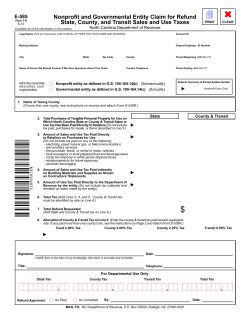


© Copyright 2026