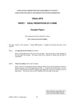
Composite Structures 57 (2002) 117–123
www.elsevier.com/locate/compstruct
A semi-analytical ﬁnite element for laminated composite plates
H.Y. Sheng a, J.Q. Ye
a
b,*
Department of Building Engineering, Hefei University of Technology, Hefei 230009, China
b
School of Civil Engineering, University of Leeds, Leeds LS2 9JT, UK
Abstract
This paper presents a semi-analytical ﬁnite element solution for laminated composite plates. The method is based on a mixed
variational principle that involves both displacements and stresses. Finite element meshes are only used in the plane of plate, while
the through thickness distributions of displacements and stresses are obtained using the method of state equations. Numerical
results show that the rate of convergence of the new method is fast and the solutions can be very close to corresponding exact threedimensional ones. The use of a recursive formulation of the state equations leads to an algebra equation system, from which solution
are sought, whose dimension is independent of the numbers of layers of the plate considered.
Ó 2002 Elsevier Science Ltd. All rights reserved.
Keywords: State equation; Three-dimensional elasticity; Laminated composite plate; Finite element
1. Introduction
Structures composed of laminated materials are
among the most important structures used in modern
engineering, and especially in the aerospace industry. Such lightweight and highly reinforced structures
are also being increasingly used in civil, mechanical
and transportation engineering applications. The rapid
increase of the industrial use of these structures has necessitated the development of new analytical and numerical tools which are suitable for the analysis and
study of the mechanical behavior of such structures.
However, the behavior of structures composed of advanced composite materials are considerably more
complicated than for isotropic materials. The strong inﬂuences of anisotropy, the transverse stresses through
the thickness of a laminate and the stress distribution at
interfaces play important roles in the performance of
such structures, since they are the main causes for interface cracking and failure. It has been recognized that
the prediction of their behavior should be based on a
three-dimensional rather than the conventional twodimensional approaches.
*
Corresponding author. Fax: +44-0113-2332265.
E-mail address: [email protected] (J.Q. Ye).
Three-dimensional analytical solutions of laminated
plates is a subject that has been extensively studied in the
last few decades [1,2]. In this respect, a recent proposed
method [3] used a recursive formulation of state equation to obtain exact solutions of laminated plates with
simply supported edges. The state equation approach
was also used by other researchers to solve vibration
problem of thick cylindrical shells [4]. The recursive
formulation of state equation was further used to deal
with laminated plates with more complex support conditions [5–7]. It was concluded from these works that the
recursive formulation of state equations for laminated
plates provides accurate three-dimensional results and
minimizes the number of unknown functions to be
solved. The solution also provides a continuous transverse stress ﬁeld across the thickness of a laminate. It
was realized, however, that to use the method for more
practical structures, a numerical realization, e.g., in the
form of ﬁnite element methods, of the recursive formulation of state equations should be established.
Conventional ﬁnite element analyses are based on a
representation of the displacement ﬁeld that guarantees the continuity of all displacements across the element boundaries. The stress ﬁeld derived from the
displacement representation by the use of the stress–
strain relations leads to a stress ﬁeld that is usually discontinuous across element boundaries. As a result, the
behavior of a multi-laminated composite cannot be
0263-8223/02/$ - see front matter Ó 2002 Elsevier Science Ltd. All rights reserved.
PII: S 0 2 6 3 - 8 2 2 3 ( 0 2 ) 0 0 0 7 5 - 2
118
H.Y. Sheng, J.Q. Ye / Composite Structures 57 (2002) 117–123
predicted satisfactorily by the three-dimensional ﬁnite
element models in use at present in general, though many
works have been done to improve the performance of
these models [8–10].
In this paper, a combination of ﬁnite element approximation and analytical solution of the recursive
formulation of state equation is proposed to solve stress
problems of laminated plates. The method is based on a
mixed variational principle that involves the variations
of both displacements and transverse stresses. The plate
is divided into ﬁnite element meshes in the plane of
plates, while the cross-thickness distributions of displacements and stresses are solved from the state equations. As observed from analytical solutions of the
state equations, the numerical solutions can also provide
continuous displacements and transverse stresses across
all material interfaces. Other features of the method
include that the dimension of the ﬁnal algebra equations
is independent of the number of material layers of a
laminate.
2. The principles of variation for three-dimensional bodies
where
T
eyy ezz eyz exz exy ; u ¼ ½u v wT
2
3
o=ox
0
0
0
o=oz o=oy
EðrÞ ¼ 4 0
o=oy
0
o=oz
0
o=ox 5
0
0
o=oz o=oy o=ox
0
e ¼ ½exx
(b) Equilibrium equations
EðrÞr þ f ¼ 0
ð2Þ
where
r ¼ ½rxx
f ¼ ½fx
ryy
fy
rzz
fz ryz
T
rxy ;
rxz
T
(c) Stress–strain relations
frg ¼ ½Qfeg
ð3Þ
where
2
C11
6 C12
6
6 C13
½Q ¼ 6
6 0
6
4 0
0
C12
C22
C23
0
0
0
C13
C23
C33
0
0
0
0
0
0
C44
0
0
0
0
0
0
C55
0
3
0
0 7
7
0 7
7:
0 7
7
0 5
C66
2.1. Three-dimensional equations of elasticity
Consider a thick rectangular plate of length a, width b
and uniform thickness h, as shown in Fig. 1. The corresponding coordinate parameters are denoted with x, y
and z, respectively, while u, v and w represent the associated displacement components. It is assumed that
the plate is made of N diﬀerent orthotropic material
layers, each of which may have diﬀerent thickness. It is
further assumed that the material axes of all these orthotropic layers coincide with the axes of the adopted
rectangular coordinate system. Hence, the fundamental
equations of an arbitrary material layer of the plate can
be written as:
(a) Strain–displacement relations
The symbols used in Eqs. (1)–(3) are deﬁned in the usual
way.
2.2. The principle of virtual displacements
The principle of virtual displacement states that a
deformable system is in equilibrium if the total external
virtual work is equal to the total internal virtual work
for every virtual displacement consistent with the constraints. Hence, for the three-dimensional problem described above, the mathematical statement of the
principle of virtual displacements is as follow:
Z Z Z
Z Z
ð4Þ
ðdeT r duT fÞ dV duT p dS ¼ 0
V
e ¼ ET ðDÞu
ð1Þ
Br
where du and de denote, respectively, virtual displacements and virtual strains. p here represents the described
tractions acting on stress boundaries (Br ) of the threedimensional body. Eq. (4) can be further written as
Z Z Z
Z Z
duT ½EðDÞr þ f dV duT ðps pÞ dS ¼ 0
V
Br
ð5Þ
where ps is the boundary stress induced by applied external forces. If stress boundary conditions are satisﬁed,
i.e., ps ¼ p, Eq. (5) has the following form:
Z Z Z
duT ½EðDÞr þ f dV ¼ 0
ð6Þ
Fig. 1. Nomenclature of a laminated rectangular plate.
V
H.Y. Sheng, J.Q. Ye / Composite Structures 57 (2002) 117–123
2.3. The principle of virtual forces
The principle of virtual forces states that the strains
and displacements in a deformable system are compatible and consistent with the constraints if the total external complementary virtual work is equal to the total
internal complementary virtual work for every system of
virtual forces and stresses that satisfy the equation of
equilibrium. On the basis of the principle, The virtual
work done by internal virtual stresses dr and virtual
tractions dps on displacement boundaries (Bu ) satisfy the
following equation.
Z Z Z
Z Z
drT e dV dpTs u dS ¼ 0
ð7Þ
V
where u is the described boundary displacement vector.
Eq. (7) can be further written as
Z Z Z
Z Z
drT ½e ET ðrÞu dV þ
dpTs ðu u dSÞ ¼ 0
V
Bu
ð8Þ
If the boundary conditions on displacement boundaries
are satisﬁed, i.e., u ¼ u, Eq. (8) becomes
Z Z Z
drT ½e ET ðrÞu dV ¼ 0
ð9Þ
V
The stress analysis in following sections uses both Eqs.
(6) and (9) simultaneously, which forms a mixed representation of the variational principles and provides the
theoretical foundation of the present method.
3. Finite element approximation in the x–y plane
To solve the stress problem of the plate shown in
Fig. 1, ﬁnite element method is used ﬁrst to discrete the
plate. In this paper, this is achieved by introducing an
isoparametric element that has the traditional ﬁnite element features in the x–y plane while the node parameters are taken as functions of z-coordinate. In more
details, the displacement and stress ﬁelds of a typical element k in the laminated plate are described as follows:
uk ¼
n
X
Nik ðn; gÞuki ðzÞ;
rkxz ¼
n
X
i¼1
rkxx ¼
n
X
i¼1
Nik ðn; gÞrkxxi ðzÞ;
n
X
vk ¼
i¼1
rkyz ¼
n
X
n
X
Nik ðn; gÞrkyzi ðzÞ;
rkyy ¼
¼
n
X
i¼1
n
X
Nik ðn; gÞrkyyi ðzÞ
i¼1
Nik ðn; gÞwki ðzÞ;
i¼1
rkxy
Nik ðn; gÞvki ðzÞ
i¼1
i¼1
wk ¼
Nik ðn; gÞrkxzi ðzÞ
rkzz ¼
n
X
i¼1
Nik ðn; gÞrkxyi ðzÞ
Nik ðn; gÞrkzzi ðzÞ
ð10Þ
119
In Eq. (10), n and g are local coordinates; Nik ðn; gÞ are
shape functions of the element and n denotes the total
node number of the element. uki ðzÞ, rkxzi ðzÞ, etc., are
functions of z and hence are called node functions of
either displacements or stresses.
4. State equation of the semi-analytical FE solutions for
single layered plates
Substitution of Eq. (10) into Eqs. (6) and (9) yields
following two variational equations that are presented
in terms of above-mentioned node functions.
T 0 B
p
dp
0 A d p
C D
q
dq
A 0 dz q
z
E
þ
fSg dz ¼ 0
F
Z
p
T
dz ¼ 0
fdSg ½GfSg ½ H Y q
z
Z ð11Þ
ð12Þ
where
fpgT ¼ ½uðzÞ vðzÞ wðzÞ;
fqgT ¼ ½rxz ðzÞ ryz ðzÞ
T
fSg ¼ ½rxx ðzÞ
rzz ðzÞ;
and
ryy ðzÞ rxy ðzÞ
are vectors composed of the node functions shown in
Eq. (10). Each node function in the vectors is arranged
in an ascent order of node number, e.g. uðzÞ ¼ ½u1 ðzÞ;
u2 ðzÞ; . . . ; uM ðzÞ, where M is the total number of nodes.
The constant matrices in above equations can be calculated as follows:
2
A
0
6
½A ¼ 6
40
A
0
0
2
0
3
7
07
5;
A
3
0 0 B
6
7
7
½C ¼ 6
4 0 0 C 5;
0 0 0
2
3
0 C
B
6
B
7
½E ¼ 4 0 C
5;
0 0 0
2
S12 A
S11 A
6 ½G ¼ 4 S12 A S22 A
2
B
4
½H ¼ 0
C
0
0
C
B
0
3
0
0 5;
0
2
0
6
½B ¼ 6
4 0
0
0
0
3
7
07
5
0
C
B
2
3
S55 A
0
0
6
7
½D ¼ 6
0 7
S44 A
4 0
5
0
0
S33 A
2
3
0
0
0
6
7
½F ¼ 4 0
0
05
S23 A
0
S13 A
3
0
7
0 5
S66 A
2
3
0 0 S13 A
5
½Y ¼ 4 0 0 S23 A
0 0
0
120
¼
½A
H.Y. Sheng, J.Q. Ye / Composite Structures 57 (2002) 117–123
m Z Z
X
Xk
k¼1
¼
½B
m
X
k¼1
¼
½C
Z Z
fNki g
Xk
m Z Z
X
k¼1
boundaries that have been prescribed by either given
stresses or given displacements. In the case that the
prescribed boundary displacements and stresses are
zeros, i.e.,
T
fNki g Nki dx dy
fNki g
Xk
oNki
ox
T
dx dy
fpo g ¼ 0;
k T
oNi
oy
ð13Þ
ð14Þ
Eliminating fSg from above two equations gives
d
fRg ¼ ½TfRg
dz
ð15Þ
T
Y
ð16Þ
Eq. (15) is called State Equation that can be solved either numerically or analytically. The solution can be
represented by
fRðzÞg ¼ ½ZðzÞfRð0Þg
ð20Þ
T
p
½GfSg ½ H Y ¼0
q
B
E
½G
1 ½ H
D
F
fSo g ¼ 0
Eq. (16) becomes
dx dy
In above matrices, the Sij are components of the compliance matrix that is obtained by inversing matrix ½Q
in Eq. (3) and Xk is the surface area of element k in the
x–y plane. Eqs. (11) and (12) involve variations of both
displacements and stresses and are called mixed variational equations.
On the basis of the principle of variation, it is evident
that Eqs. (11) and (12) are equivalent to following sets of
equation system:
p
E
0 B
0 A d p
þ
fSg ¼ 0
q
F
C D
A 0 dz q
where fRg ¼ ½p; q
1 0 A
0
½T ¼
A 0
C
fqo g ¼ 0;
ð17Þ
where fRð0Þg is the value of fRðzÞg at z ¼ 0. If Eq. (15)
is solved analytically, matrix ½ZðzÞ is in following form:
½ZðzÞ ¼ ½Pdiag ek1 z ek2 z . . . ekK z ½P
1
ð18Þ
in which, the kj ( j ¼ 1; 2; . . . ; K) are distinct eigenvalues
of matrix ½T and ½P is the associated matrix consisting
of corresponding eigenvectors. In the case of repeated
eigenvalues, analytical solutions of (16) can also be
sought [11].
To facilitate the introduction of boundary conditions,
the node function vectors in Eqs. (11) and (12) may be
partitioned into two parts as shown below,
pf
qf
Sf
fpg ¼
; fqg ¼
; fSg ¼
ð19Þ
po
qo
So
where pf , qf and Sf include all unknown node functions
while po , qo and So are the node functions along the
R ¼ ½pf ; qf 1 0 Af
0
½T ¼
ATf
0
Cf
Bf
Df
Ef
Ff
1
½Gf ½ Hf
Yf ð21Þ
in which only matrices associated with the unknown
node functions are involved. The solution of Eq. (15)
can then be found by following the solution procedure
described by Eqs. (17) and (18). It should be mentioned
here is that the boundary conditions discussed above are
only the conditions imposed on the four edges of the
plate. The stress and displacement conditions on the top
and bottom surfaces of the plate are treated in Section 5.
5. Solutions of state equations for laminated plates
Consider the N-plied laminated plate composed of
orthotropic layers (see Fig. 1). For the jth layer having
thickness hj , the state equation and its solution are
found, respectively, in the form of Eqs. (15) and (17),
i.e.,
d
fRj ðzÞg ¼ ½Tj fRj ðzÞg 0 6 z 6 hj
dz
fRj ðhj Þg ¼ ½Zj ðhj ÞfRj ð0Þg
ð22Þ
ð23Þ
The continuity condition at interfaces of the laminate
requires continuous ﬁelds of both displacements and
transverse stresses. This condition can be satisﬁed by
imposing following relations at each interface:
fRjþ1 ð0Þg ¼ fRj ðhj Þg
ðj ¼ 1; 2; . . . ; N 1Þ
ð24Þ
Hence, upon recursively using Eqs. (23) and (24), the
following equation can be found for the N-layered
composite plate.
fRN ðhN Þg ¼ ½ZN ð0ÞfRN ð0Þg ¼ ½TN ð0ÞfRN 1 ðhj
1 Þg
¼ ½ZN ðhN Þð½ZN 1 ðhN 1 ÞfRN
1 ð0ÞgÞ
¼ ¼ ½PfR1 ð0Þg;
where,
"
½P ¼
1
Y
ð25Þ
#
ð½Zk ðhk ÞÞ ;
ð26Þ
k¼N
which is equivalent to the ½Z matrix in Eq. (17). In Eq.
(25), RN (hN ) and R1 ð0Þ are the node function vectors
consisting of displacements and transverse stresses on
the bottom (Z ¼ h) and top (Z ¼ 0) lateral surfaces of
H.Y. Sheng, J.Q. Ye / Composite Structures 57 (2002) 117–123
the laminated plate, respectively. By introducing load
conditions on the two lateral surfaces into Eq. (25), a set
of linear algebra equations in terms of node displacement functions are formed, from which the solutions of
the problem can be obtained. It is worthwhile to mention that the dimension of Eq. (25) is identical to that of
Eq. (17). Hence, it can be concluded that the dimension
of Eq. (25) depends solely on the ﬁnite element meshes
used in the x–y plane and is completely independent of
the number of layers of the composite plate considered.
In the case of uniformly distributed pressure, x, applied on the top surface of the laminated plate, for instance, the corresponding load conditions on the lateral
surfaces are:
T
fqf ð0Þg1
¼ ½rxz ð0Þ
fqf ðhN ÞgTN
ryz ð0Þ
¼ ½rxz ðhÞ
ryz ðhÞ
rzz ð0Þ ¼ ½0
0
rzz ðhÞ ¼ ½0
x
ð27Þ
The subscripts 1 and N here indicate that the node
function vectors are of the top and bottom layers, respectively. Substituting Eq. (27) into (17) for singlelayered plates or into (25) for multi-layered ones yields
following linear algebra equations:
9
2
38
2
3
P41 P42 P43 < uf ð0Þ =
P46
4 P51 P52 P53 5 vf ð0Þ
ð28Þ
¼ 4 P56 5fxg
:
;
wf ð0Þ 1
P61 P62 P63
P66
where the Pij are relevant sub-matrices from P in Eq.
(25) and fxg is the external loads applied at the nodes
on the top surface of the plate. Once the initial values of
the node displacement functions, i.e. the values of node
displacements at z ¼ 0 are found, the displacements and
121
stresses at any location throughout the thickness can be
calculated using Eqs. (17) and (23).
6. Numerical examples
To validate the new method, numerical calculations
are carried out for a three-plied square plate with simply
supported edges. The plate has two identical face layers
and a core layer that have the same ratios of stiﬀnesses
as follows:
C12 =C11 ¼ 0:246269
C22 =C11 ¼ 0:543103
C13 =C11 ¼ 0:0831715
C23 =C11 ¼ 0:115017
C33 =C11 ¼ 0:530172
C44 =C11 ¼ 0:266810
C55 =C11 ¼ 0:159914
C66 =C11 ¼ 0:262931
The face and core layers are distinguished by the ratio
ðFÞ
ðCÞ
d ¼ C11 =C11 , where F and C denote face and core,
respectively. The plate has a total thickness of h, of
which the thickness of each face layer is 0.1h. The plate
is subjected to a uniformly distributed pressure, q, on the
top surface. The plate was ﬁrst used by Srinivas and Rao
[1] and then used by Fan and Ye [3] in their three-dimensional modeling. As a result of symmetry, only a
quarter of the plate is analyzed in the following calculations. Eight-node quadrilateral elements are used in
the x–y plane while the state equations are solved analytically. The convergence rate of the new method is
assessed by calculating displacements and stresses
against various ﬁnite element meshes. These displacements and stresses are calculated for a thick sandwich
Table 1
Convergence rate of the semi-analytical FE method
u (x ¼ 0,
y ¼ a=2)
v (x ¼ a=2,
y ¼ 0)
(x ¼ a=2,
w
y ¼ a=2)
rxx (x ¼ a=2,
y ¼ a=2)
ryy (x ¼ a=2,
y ¼ a=2)
rxz (x ¼ 0,
y ¼ a=2)
11
Tþ
T
Bþ
B
0.26375
0.07486
0.03677
0.09293
0.44304
0.08949
0.17884
0.30892
1.62456
1.59831
0.75508
0.74388
2.34013
0.27353
0.07179
1.40245
2.13727
0.84006
0.78321
1.65716
0.00000
0.51814
0.38167
0.00000
22
Tþ
T
Bþ
B
0.32882
0.10569
0.04201
0.10346
0.53870
0.07594
0.20244
0.34668
1.72879
1.70376
0.85513
0.84266
2.20675
0.45209
0.08709
1.54869
2.11390
0.96724
0.87593
1.85248
0.00000
0.74035
0.31625
0.00000
33
Tþ
T
Bþ
B
0.33783
0.11111
0.04210
0.10382
0.55009
0.06820
0.20267
0.34716
1.73447
1.70928
0.85515
0.84268
2.23342
0.43870
0.08766
1.54723
2.12707
0.96899
0.87667
1.85021
0.00000
0.80195
0.31766
0.00000
44
Tþ
T
Bþ
B
0.33915
0.11178
0.04203
0.10370
0.55190
0.06621
0.20238
0.34664
1.73710
1.71179
0.85383
0.84139
2.25129
0.42755
0.08722
1.54520
2.13720
0.96544
0.87528
1.84736
0.00000
0.82050
0.31720
0.00000
Mesh
ð29Þ
122
H.Y. Sheng, J.Q. Ye / Composite Structures 57 (2002) 117–123
plate having h=a ¼ 0:6 and d ¼ 5. The results are shown
in Table 1 as the non-dimensional parameters deﬁned
below:
C ðCÞ
¼ 11 ð u
u v w
qh
¼ ð rxx
ryy
v wÞ
rxx
ryy
rxz Þ=q
rxz
ð30Þ
In the table, T denotes top layer and B denotes bottom
layer. þ and indicate, respectively, top and bottom
surfaces of a layer. From the results shown above, it is
evident that the solutions convergent very fast for both
displacements and stresses.
After the convergence test, the new method is further
used to analyze the same plate used above except that
the thickness ratio varies. The results are obtained by
use of 3 3 meshes and the displacements and stresses
at the two lateral surface and the two interfaces are
presented in Table 2, where Cþ and C
denote the top
and bottom surfaces of the core layer. Exact solutions of
the problems [3] are also given in the table for comparisons. The comparisons show that the numerical results obtained by using the new method have an
excellent agreement with the exact ones for all the displacements and stresses shown except the transverse
stress rxz at the up interface of the thin plate (h=a ¼ 0:2).
The discrepancies observed is attributed to the fact that
for the thin plate the up interface is close to the top
surface where external pressure is applied. The discrepancies become insigniﬁcant as the plate becomes thicker,
i.e. as the distance between the top surface and the up
interface increases.
Table 2
Stress and displacements of laminated plates with various values of h=a
h=a ¼ 0:2
Present
h=a ¼ 0:4
h=a ¼ 0:6
Exact
Present
Exact
Present
Exact
u (x ¼ 0, y ¼ a=2)
Tþ
T
Cþ
C
Bþ
B
4.29409
2.45837
2.45837
2.52127
2.52127
4.12774
4.30597
2.41992
2.41992
2.50837
2.50837
4.10213
0.66780
0.00974
0.00974
0.06279
0.06279
0.43153
0.67331
0.00445
0.00445
0.06268
0.06268
0.42902
0.33783
0.11111
0.11111
0.04210
0.04210
0.10383
0.34047
0.11156
0.11156
0.04187
0.04187
0.10330
v (x ¼ a=2, y ¼ 0)
Tþ
T
Cþ
C
Bþ
B
6.05486
4.21700
4.21700
4.62386
4.62386
6.20999
6.06895
4.16141
4.16141
4.59869
4.59869
6.17415
1.18281
0.50281
0.50281
0.70180
0.70180
1.06011
1.18974
0.49068
0.49068
0.69832
0.69832
1.05490
0.55009
0.06820
0.06820
0.20267
0.20267
0.34716
0.55305
0.06572
0.06572
0.20169
0.20169
0.34548
w
(x ¼ a=2, y ¼ a=2)
Tþ
T
Cþ
C
Bþ
B
24.22580
24.27650
24.27650
23.52280
23.52280
23.43120
24.16525
24.21478
24.21478
23.44410
23.44410
23.35246
3.74259
3.72933
3.72933
2.93253
2.93253
2.90558
3.74815
3.73390
3.73390
2.92013
2.92013
2.89325
1.73447
1.70928
1.70928
0.85515
0.85515
0.84268
1.73959
1.71354
1.71354
0.85107
0.85107
0.83866
rxx (x ¼ a=2, y ¼ a=2)
Tþ
T
Cþ
C
Bþ
B
14.56300
10.03420
2.12548
2.01035
10.08070
14.51690
14.57415
10.01557
2.12383
2.00427
10.05120
14.52536
3.72026
1.63015
0.44427
0.27924
1.42938
3.53944
3.77946
1.62159
0.44496
0.27671
1.41743
3.53638
2.23342
0.43870
0.20763
0.00959
0.08766
1.54723
2.31852
0.40611
0.20352
0.00930
0.08623
1.54147
ryy (x ¼ a=2, y ¼ a=2)
Tþ
T
Cþ
C
Bþ
B
10.80440
7.92558
1.74920
1.61927
8.13637
10.95310
10.81844
7.91679
1.75029
1.61725
8.12754
10.96442
3.51125
2.13518
0.59054
0.43973
2.24452
3.66155
3.54854
2.13820
0.59447
0.43749
2.23433
3.65116
2.12707
0.96899
0.35960
0.16435
0.87667
1.85021
2.18497
0.95508
0.36014
0.16346
0.87228
1.84165
rxz (x ¼ a=2, y ¼ a=2)
Tþ
T
Cþ
C
Bþ
B
0.00000
1.72495
1.72495
1.54285
1.54285
0.00000
0.00000
1.92682
1.92682
1.52792
1.52792
0.00000
0.00000
1.00113
1.00113
0.63519
0.63519
0.00000
0.00000
1.08471
1.08471
0.62979
0.62979
0.00000
0.00000
0.80195
0.80195
0.31766
0.31766
0.00000
0.00000
0.83821
0.83821
0.31585
0.31585
0.00000
H.Y. Sheng, J.Q. Ye / Composite Structures 57 (2002) 117–123
7. Concluding remarks
A semi-analytical ﬁnite element method has been
presented to solve three-dimensional stress problems of
laminated plates having orthotropic material layers. The
method was based on a mixed variational representation
of the three-dimensional equations of elasticity. The inplane ﬁelds of both displacements and stresses are approximated by ﬁnite elements while their through
thickness distributions were obtained by solving state
equations.
Numerical tests have been carried out to show the
convergence rate and accuracy of the method. It was
observed that the rate of convergence of the method is
very fast and the results obtained had excellent agreement with the exact solutions of the problems available
in the literature.
Since the recursive formulation was used to derive the
state equations of laminated plates, the dimension of the
ﬁnal state equations was independent of the layer
number of the plates. As a result, this method is particularly suitable to solve stress problems of multilayered composite panels. The method always provides
a continuous distribution of both displacements and
transverse stresses across material interfaces of the
laminated plates.
Acknowledgements
The second author wishes to thank the School of
Mechanical and Production Engineering at Nanyang
123
Technological University, Singapore for the support he
received as a Tan Chin Tuan Engineering Fellow.
References
[1] Srinivas S, Rao AK. Bending vibration and buckling of simply
supported thick orthotropic rectangular plates and laminates. Int
J Solid Struct 1970;6:1463–81.
[2] Rogers TG, Waston P, Spencer AJ. An exact three-dimensional
solution for normal loading of inhomogeneous and laminated
anisotropic elastic plates of moderate thickness. Proc R Soc Lond
A 1992;437:199–213.
[3] Fan JR, Ye JQ. An exact solution for the statics and dynamics of
laminated thick plates with orthotropic layers. Int J Solids Struct
1990;26(5/6):655–62.
[4] Soldatos KP, Hadjigeorgiou VP. Three-dimensional solution of
the free vibration problem of homogeneous isotropic cylindrical
shells and panels. J Sound Vibr 1990;137:369–84.
[5] Fan JR, Sheng HY. Exact solution for thick laminates with
clamped edges. Acta Mechanica Sinica 1992;24:574–83.
[6] Ye JQ, Soldatos KP. Three-dimensional vibration of laminated
composite plates and cylindrical panels with arbitrarily located
lateral surfaces point supports. Int J Mech Sci 1996;38(3):271–
81.
[7] Ye JQ. A free vibration analysis of cross-ply laminated rectangular plates with clamped edges. Comput Meth Appl Mech Engng
1997;140(3–4):383–92.
[8] Noor AK, Peters JM. Stress, vibration, and buckling of multilayered cylinders. J Struct Engng ASCE 1989;115:69–88.
[9] Noor AK, Burton WS. Assessment of Computational models for
of multi-layered Composite shells. Appl Mech Rev 1990;43:67–
97.
[10] Reddy JN. An evaluation of equivalent-single-layer and layerwise
theories of composite laminates. Compos Struct 1993;25:21–35.
[11] DeRusso PM, Roy RJ, Close CM. State variables for engineers.
New York: John Wiley; 1995.