Support Vectors Selection by Linear Programming
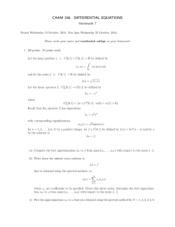
Vojislav Kecman, Ivana Hadzic
Department of Mechanical Engineering, University of Auckland,
Private Bag 92019, Auckland, New Zealand
E-mail: [email protected]
Abstract
A linear programming (LP) based method is proposed for learning from experimental data in solving the nonlinear
regression and classification problems. LP controls both the number of basis functions in a neural network (i.e.,
support vector machine) and the accuracy of learning machine. Two different methods are suggested in regression
and their equivalence is discussed. Examples of function approximation and classification (pattern recognition) illustrate the efficiency of the proposed method.
Keywords: support vector machines, neural networks, linear programming, learning from experimental data, nonlinear multivariate functions approximations, nonlinear multivariate pattern recognition
1.
Introduction
Support Vector Machine (SVM) is a new type of learning machine that keeps the training error fixed (i.e., within
given boundaries), and minimizes the confidence interval, i.e., it matches the machine capacity to data complexity.
SVM that uses quadratic programming (QP) in calculating support vectors has very sound theoretical basis and it
works almost perfectly for not too large data sets. When the number of points is large (say more then 2000), the QP
problem becomes extremely difficult to solve with standard methods and program solvers. Recently, a lot of work
was done on implementing an LP approach in support vectors selection. Kecman (1999) suggested optimal subset
selection by using LP in solving regression tasks by minimizing the L1 norm of the output layer weight vector w.
Hadzic and Kecman (1999) implemented such an LP approach to classification problems. Zhang and Fuchs (1999)
proposed an LP based method for selecting the hidden neurons at the initialization stage of the multilayer perceptron
network. The LP approaches in solving regression problems have been implemented since 1950ties (see Charnes,
Cooper and Ferguson 1955, Cheney and Goldstein 1958a, Stiefel 1960, Kelley 1957, Rice 1964). These results follow from minimizing L1 norm of an error. (Interestingly, the first results on the L1 norm estimators were given as
early as 1757 by Yugoslav scientist Boskovic, see Eisenhart, 1962). The summary and very good presentations of
mathematical programming application in statistics were given by Arthanari and Dodge (1993). An early work on LP
based classification algorithms dates back to the middle of 1960s (see Mangasarian 1965). Recently, a lot of work
has been done on implementing LP approach in support vectors selection (Smola et all 1998, Bennett 1999, Weston
et all 1999, and Graepel et all 1999). All these papers originate from the same stream of ideas clustered around controlling the (maximal) margin. Hence, they are close to the SVM constructive algorithms.
We demonstrate the LP based approach by using the regression examples and we expand the same method for solving classification tasks. Here, the slight difference in respect to the standard SVM learning is that instead minimizing
L2 norm ||w||2 of the weight vector w, we will minimize L1 norm ||w||1 in an LP approach. In Section 2, we develop
two methods for solving regression problems by LP and discuss their equivalence. In Section 3, an LP approach is
expanded for solving classification tasks. Section 4 is devoted to simulation examples, and some conclusions are
drawn in Section 5.
2. Linear Programming in Regression
Minimization of the L2 norm equals minimizing wTw =
∑
n
i =1
wi = w1 + w2 + " + wn and this results in the QP type
2
2
2
2
of problem that leads to a maximization of a margin M (Vapnik, 1995). Here, instead minimizing an L2 norm of the
weight vector w we will minimize its L1 norm. The geometrical meaning of the L1 norm is not clear yet but the appli-
cation of the LP approach for a subset (support vectors, basis functions) selection results in a very good performance
of NN and/or SVM. At the same time there is no theoretical evidence either that, the minimization of the L1 norm or
L2 norm of the weight vector w produces superior generalization.
2.1
Sparseness regularization method
Regression tasks could be formulated in many different ways. Here we show two approaches. First method is a oneobjective function minimization problem and the second one is a multi-objective function minimization task. Our
problem is to design a parsimonious NN containing less neurons than data points. Such a sparseness of an NN or
SVM results from minimizing L1 norm of the weight vector w. At the same time, we want to solve y = Gw such that
|| Gw – y || is small for some chosen norm. In order to perform such a task we formulate the regression problem as
follows - find a weight vector
w = arg min||w||1,
| Gw – y ||∞ ≤ ε,
subject to,
(1)
where ε defines the maximally allowed error (that is why we used L∞ norm) and corresponds to the ε-insensitivity
zone in an SVM learning. This constrained optimization problem can easily be transformed into a standard linear
programming form. First, recall that min||w||1 = min ∑ p =1 | w p | , and this is not an LP problem formulation where we
P
∑
typically minimize cTw =
P
p =1
c p w p and c is some known coefficient vector. (P denotes the number of training
data). Thus, in order to apply the LP algorithm we use the standard trick by replacing wp and | wp | as follows
+
−
wp = w p - w p
+
+
(2a)
−
|wp| = w p + w p
−
+
(2b)
−
where w p and w p are the two non-negative variables, i.e., w p ≥ 0, w p ≥ 0. Note, that the substitutions done in (2)
+
−
are unique, i.e., for a given wp there is only one pair ( w p , w p ) which fulfills both equations. Furthermore, both variables can not be bigger than zero at the same time. In fact there are only three possible solutions for a pair of vari+
−
+
−
ables ( w p , w p ), namely, (0, 0), ( w p , 0) or (0, w p ). Second, the constraint in (1) is not in a standard formulation either and it should also be reformulated as follows. Note that || Gw – y ||∞ ≤ ε in (1) defines an ε-tube inside which
should our approximating function reside. Such a constraint can be rewritten as
y - ε 1 ≤ Gw ≤ y + ε 1
(3)
where 1 is a (P, 1) column vector filled with ones. Equation (3) represents a standard set of linear constraints and our
LP problem to solve is now the following. Find a pair
P
(w ,w ) = arg min ∑ ( w p +w p ) , subject to, y - ε 1 ≤ G(w - w ) ≤ y + ε 1, (4a), w ≥ 0, (4b), w ≥ 0, (4c)
+
−
+
+
−
−
+
−
p =1
+
+
+
+
−
−
−
−
where w = [ w1 , w2 ," , wP ]T and w = [ w1 w2 . . . wP ]T. LP problem (4) can be presented in a matrix-vector
formulation suitable for an LP solver as follows: min cTw, i.e.,
w
min 1 1 ... 1

w

P columns
+
+
−
−
− T
 + +
1 1 ... 1  w1 w2 " wP w1 w2 " wP 

P columns
 G
subject to, 
 −G
− G  w 
+
 y + ε 1
≤
, (5)


G   w −   − y + ε 1 
−
w ≥ 0, w ≥ 0,
where both w and c are the (2P, 1)-dimensional vectors. c = 1(2P, 1), and w = [w
(6), (7)
+T
−
w T]T.
2.2
Expanded sparseness regularization method
Here, the original problem is not changed in the sense that we want to solve y = Gw such that ||Gw – y|| is small for
some chosen norm. However, the formulation is different. Instead of minimizing ||w||1 that enforces a model sparseness only, we additionally require that the Chebyshev norm Gw − y ∞ is minimal as well. In other words, we want
to minimize the ε-tube inside which our regression function reside. Thus, we want to minimize regularized risk
Rreg = λ ||w||1 + C1 Gw − y ∞ .
(8)
If we divide (8) with λ an optimal solution doesn’t change and regularized risk functional becomes
Rreg = 1 ||w||1 + C Gw − y
(9)
∞
Same as in section 2.1 we introduce new variables w+ and w-. Second term on the RHS of our objective function (9)
is not in a standard LP formulation either. Let’s introduce new variables ri + , ri − (Rice, 1964)
+
ri = yi − G i w + d ,
(10)
−
ri = −( yi − G i w ) + d
+
−
where Gi denotes the i-th row of the design matrix G, r-s are deviations such that ri , ri ≥ 0 , yi is the known observation and d is maximal deviation of the approximation, i.e.,
d ≥ − ( yi − G i w )
(11),
d ≥ yi − G i w
where i = 1, 2, …, P, or
d ≥ max yi − G i w
(12)
i
The problem may now be reformulated as follows. Minimize d subject to the 2P constraints ri + , ri − ≥ 0. d is equivalent to the ε in the sparseness regularization method presented in 2.1. Linear programming problem now becomes
min
[1
1
w ,d
+
C ]  w
+
w
−
d  , subject to,
T
 G -G -1 +
 −G G -1  w


−
w ≥ 0, w ≥ 0, d ≥ 0
w
−
T
 y
d  ≤   ,
−y 
(13)
(14), (15), (16)
Proposition: If expanded sparseness regularization leads to the solution w , d then sparseness regularization with ε
set apriori to d and with same parameters for basis functions, has the solution w .
Proof: It is easy to show that for a fixed d = ε, equation (13) is equal to (5).
Since both methods lead to the same optimal solution, we present only first method in simulation examples section.
3. Linear Programming in Classification
The supervised learning algorithm embedded in a learning machine (which can be any of these - multilayer perceptron NN, SV machine, RBF network or neuro-fuzzy model) typically learns the separation boundary f(x) by using a
training data set D = {[x(i), y(i)] ∈ ℜn × ℜ, i = 1,...,P} consisting of P pairs (x1, y1), (x2, y2), …, (xP, yP), where the
inputs x are n-dimensional vectors (x ∈ ℜ n) and the class labels y are discrete (e.g., Boolean) values for classification problems. yi are also called the desired values in classic supervised learning. Here, because of space constraints
we do not present a full derivation of the LP based learning in the case of classification. Instead, we give only the
final expressions for designing linear and nonlinear separation boundaries between classes. An LP learning algorithm for linear classification is given below
min ∑ i =1 ( wi + wi ) + C ∑ i =1 ξ i ,
P
+
−
P
yi f (xi ) ≥ 1 − ξ i
subject to,
(17)
wi + , wi− , ξ i ≥ 0
where f(xi) = wTxi + b and ξi measures the deviation of a data point from the ideal condition of pattern separability. It
corresponds to the slack variable in a classic QP learning in SVMs. In a matrix notation, matrix of input data X is
augmented by a constant input +1, i.e., X=[x1T 1; x2T 1; …, xPT 1] and bias b becomes the n + 1-st component of
the weights vector w. For a two-dimensional feature vector x, LP learning algorithm is given below,
min[1 1 0 1 1 0 C1(1, P )]  w1
+
+
w2
+
−
w3
w1
−
w2
−
w3
w+ 
 
− diag ( y ) X I( P )]  w −  ≥ 1( P,1) (18)
ξ 
 
ξ  , s.t., [diag ( y ) X
T
A trade-off constant C is a design parameter that is typically adjusted separately during the design experiments.
Classes that have nonlinear separating (hyper)boundaries have classifier constructed from some (in the case of LP
approach, not necessarily kernel) basis functions. Here, we use a polynomial (which is, by chance, a kernel function)
having ‘design matrix’ G. The LP learning formulation for a nonlinear classification tasks is given as
+
min[1(1, P ) 0 1(1, P ) 0]  w1
+
w1
+
" wP +1
−
w1
−
w2
−
" wP +1  , s.t., [diag ( y )G
T
w+ 
≥ 1( P,1) (19)
−
w 
− diag ( y )G ] 
Similarly to (18), in a nonlinear classification formulation given by (19), one can also introduce ξi variable and its
regularizing i.e., trade-off parameter C. However, this should be done with the care. Actually, the impact of such
regularization is, at the moment, under research in Hadzic (1999).
4. Simulation Examples
One-dim ensional LP based SVs selection in regression
3
1.5
y
Two dimensional LP based SVs selection in a classification
by 3rd order polynomial
x2
2.5
1
2
0.5
1.5
0
1
-0.5
0.5
-1
0
-0.5
-4
-2
0
2
x
4
Figure 1. Nonlinear regression: The SVs selection
based on an LP algorithm (5). Hermitian function f(x) =
1.1(1 – x + 2x2)exp(-0.5x2) (dashed) is polluted with a
10% Gaussian zero-mean noise. So obtained training set
contains 41 training data points (crosses). An LP algorithm has selected 10 SVs shown as encircled data
points. Resulting approximation curve (solid). Insensitivity
zone is bounded by dotted curves.
-1.5
0
x1
2
4
6
8
Figure 2. Nonlinear Classification, i.e., Pattern Recognition: The SVs selection based on an LP learning
algorithm (19). Separation boundary is sinus function
(dashed). Data are shown as crosses. Selected SVs are
shown as encircled crosses. Out of 40 training data 8
were selected as SVs. Resulting separation boundary
curve (solid).
NONLINEAR REGRESSION
In Fig 1, the SVs selection based on an LP learning algorithm (5) is shown for a Hermitian function f(x) = 1.1(1 – x
+ 2x2)e(-0.5x2) polluted with a 10% Gaussian zero-mean noise. The training set contained 41 training data pairs and
the LP algorithm has selected 10 data points as the SVs shown as encircled crosses. Basis functions are Gaussians
G(xi, cj = xj) =exp(-0.5|| xi - cj||2/(σ)2) where σ = kS∆c where ∆c denotes the average distance between the adjacent
centers of the basis functions. The resulting graph is similar to the standard QP based learning outcomes.
It was interesting to see differences between an LP and QP approach in solving regression problems. We investigated
sinus function polluted with 20% noise. In a QP solution, an insensitivity zone was chosen to be e = 0.1, C = 20⋅106
and the Gaussian bells parameter σ = 3∆c, (i.e., kS = 3). Simulations were repeated on randomly selected data set one
hundred times. Comparison of QP and LP based training algorithms shows that as number of training data increases
computational time becomes significantly smaller for LP then for QP and that the number of chosen support vectors
for LP is almost half their number for QP. At the same time, however, accuracy is slightly better for QP based algorithms. Compare a magnitude of the accuracy difference between the QP and the LP learning algorithms in the example on gender recognition below.
NONLINEAR CLASSIFICATION
Results for a nonlinear classification example are presented through a decision boundary estimation of the data belonging to two different classes separated by x2 = sin(x1). Here, the (kernel) function is the 3rd order polynomial. Despite the fact that the training data a polluted by 25% noise, resulting decision boundary, as seen in Fig. 2, is a good
approximation to a sinus separation boundary curve and data are correctly classified.
The last example is a gender recognition task as given in Brunelli and Poggio, 1993 and in Poggio and Girosi, 1993.
Data base contains 168 data pairs comprising 18-dimensional input vector x and one dimensional output +1 and –1
for male and female class respectively. Two typical faces are given in Fig 3. An input vector x comprises 18 geometrical features as given in Fig. 4. The results obtained in the Brunelli and Poggio’s paper by applying (Hyper)Gaussian Basis Function Networks are as follows: a) on the vectors of the training set (classification is 90% correct), b) on novel faces of people in the training set (86% correct) and c) on faces of people not represented in the
training set (79% correct). Human performance on all data sets was (90%). Our first results by applying QP and LP
based learning are better in all three cases. For example, on novel faces of people not represented in the training set,
QP based method was (96.4% correct) while an LP based method as given by (19) was (92,8% correct). Note that
both the QP and the LP approach outperform human performance.
Figure 3. Typical photos of male and female face without
gender facial hair used in gender classification experiments
Nr
Feature
1
2
3
4
5
6
7
8–13
14
15
16
17
18
pupil to nose vertical distance
pupil to mouth vertical distance
pupil to chin vertical distance
nose width
mouth width
zygomatic breadth
bigonial breadth
chin radii
mouth height
upper lip thickness
lower lip thickness
pupil to eyebrow separation
eyebrow thickness
Figure 4. Geometrical features (white) used in
classification and their description. (Both figures
are from Poggio and Girosi, 1993).
5. Conclusions
In this paper, we present an LP approach for solving nonlinear regression and classification tasks. For a regression,
we introduced two methods – sparseness and expanded sparseness regularization method. In the case of nonlinear
classification, we presented two LP problem formulations – first one for a calculation of a separation hyperplane and
the second formulation is aimed at calculating nonlinear separation hypersurface between two classes. The approach
and results show that an LP based learning (that resulted from the minimization of the L1 norm of the weight vector
w) produces sparse networks. This may be of particular interest in modern days applications while processing a huge
amount of data (say several dozens of thousands) that can not be processed by the contemporary QP solvers. The
results presented here are inconclusive in the sense that much more investigations and comparisons with a QP based
SVs selection on both real and ‘artificial’ data sets should be done. Despite the lack of such an analysis yet, our first
simulational results show that the LP subset selection may be more than a good alternative to the QP based algorithms when faced with a huge training data sets. Saying that we primarily refer to the following possible benefits of
applying LP based learning: a) LP algorithms are faster and more robust than QP ones, b) they tend to minimize
number of weights (meaning SV) chosen, and c) they naturally incorporate the use of kernels for creation of nonlinear separation and regression hypersurfaces in pattern recognition and function approximation problems respectively.
6.
References
Arthanari, T. S., Y. Dodge, 1993. Mathematical Programming in Statistics, J. Wiley & Sons., New York, NY
Bennett, K., 1999. Combining support vector and mathematical programming methods for induction. In B.
Schölkopf, C. Burges, and A. Smola, Editors, Advances in Kernel Methods - SV Learning, pp 307–326, MIT Press,
Cambridge, MA
Brunelli, R., T. Poggio, 1993. Caricatural Effects in Automated Face Perception, Biological Cybernetics, 69: 235241
Charnes, A., W. W. Cooper, R. O. Ferguson, 1955. Optimal Estimation of Executive Compensation by Linear
Programming, Manage. Sci., 1, 138
Cheney, E. W., A. A. Goldstein, 1958. Note on a paper by Zuhovickii concerning the Chebyshev problem for linear
equations. J. Soc. Indust. Appl. Math., Volume 6, pp. 233-239
Eisenhart, C., 1962. Roger Joseph Boscovich and the Combination of Observationes, Actes International Symposium on R. J. Boskovic, pp. 19-25, Belgrade-Zagreb-Ljubljana, YU
Graepel, T., R. Herbrich, B. Schölkopf, A. Smola, P. Bartlett, K.–R. Müller, K. Obermayer, R. Williamson,
1999. Classification on proximity data with LP–machines, Proc. of the 9th Intl. Conf. on Artificial NN, ICANN 99,
Edinburgh,7-10 Sept.
Hadzic, I., 1999. Learning from Experimental Data by Linear Programming Selected Support Vectors, PhD Thesis,
(work in progress), The University of Auckland, Auckland, NZ
Hadzic, I., V. Kecman, 1999. Learning from Data by Linear Programming, NZ Postgraduate Conference Proceedings, Auckland, Dec. 15-16
Kecman, V., 1999. Learning and Soft Computing by SVM, NN and FLS, The MIT Press, (in print), Cambridge, MA
Kelley E. J. jr., 1958. An application of linear programming to curve fitting (received by editors October 11, 1957),
J. Soc. Indust. Appl. Math., Volume 6, pp. 15-22
Mangasarian, O. L., 1965. Linear and Nonlinear Separation of Patterns by Linear Programming, Operations Research 13, pp. 444-452.
Poggio, T., F. Girosi, 1993. Learning, Approximation and Networks, Lectures and Lectures’ Handouts - Course
9.520, MIT, Cambridge, MA,
Rice R. J., 1964. The Approximation of Functions, Addison - Wesley Publishing Company, Reading, Massachusetts, Palo Alto, London
Smola A., T. T. Friess, B. Schölkopf, 1998. Semiparametric Support Vector and Linear Programming Machines,
NeuroCOLT2 Technical Report Series, NC2-TR-1998-024
Smola, A., B. Schölkopf, G. Rätsch, 1999. Linear Programs for Automatic Accuracy Control in Regression, submitted to ICANN'99
Stiefel, E., 1960. Note on Jordan Elimination, Linear Programming and Chebyshev Approximation, Numer. Math.,
2, 1.
Vapnik, V. N., 1995. The Nature of Statistical Learning Theory, Springer Verlag Inc, New York, NY
Weston, J., A. Gammerman, M. O. Stitson, V. Vapnik, V. Vovk, C. Watkins, 1999. Support Vector Density Estimation, In B. Schölkopf, C. Burges, and A. Smola, Editors, Advances in Kernel Methods - SV Learning, p.p. 307–
326, MIT Press, Cambridge, MA
Zhang, Q. H., J.-J. Fuchs, 1999. Building neural networks through linear programming, Proceedings of 14th IFAC
Triennial World Congress, Vol. K, pp. 127-132, Pergamon Press