1. No category

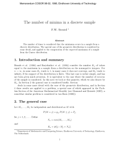
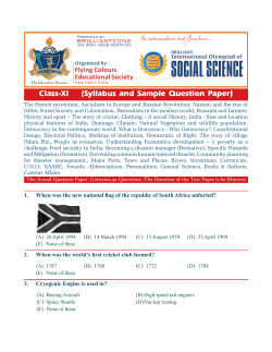
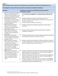
Symbolic tools for
a concrete problem of mechanic B. Mourrain
INRIA (SAFIR)
2004 Route des Lucioles
06565 Valbonne (France)
[email protected]
Abstract
In this paper, we consider the direct kinematic problem of a parallel robot (called the
Stewart platform or left hand) from a mathematical point of view. We do not try to give
real time and numerical solutions to this problem but describe tools of eective algebra,
which can help us to know a little more about the geometry of the question. A simple
proof that the number of solutions we are expecting is actually 40 is then given, using
Bezouts' theorem on spheres. One main obstacle in the natural approach, via symbolic
computations, is the great size of the polynomials that appears during the computations.
We also try to show how the use of invariant theory and intrinsic approach can "factorize"
the results in a more understandable way.
The mechanism of the Stewart Platform (or left hand) is the following. Consider six xed
points (Xi )1i5 (of a xed solid SX ) and six other points Zi , attached to a moving solid SZ .
The articulations between the two solids SX and SZ are extensible bars (Xi; Zi)1i6 with
spherical joints.
Z4
Z3
X4
X3
Z5
Z2
X5
X2
Z1
Z6
X6
X1
work partially motivated by PoSSo, EEC ESPRIT BRA contract 6846.
1
Changing the length of the bars suces to do a little deplacement of the platform. The
name "left hand" comes from the fact that this mechanism is well-suited to doing precise
movements of adjustment, as opposed to the right hand which generally does greater movements. Just think at what you do when you want to hammer a nail 1 : : : For more informations
on parallel robots, see [11].
From a practical point of view, it is easy to mesure the length of these articulations but
much less obvious to determine the position of the solid SZ , knowing these lengths.
The main purpose of this section will be to study the map which associates to a deplacement of the solid SZ , the square of the length kXi; Zik2 .
1 A rational map, its ber, its critical locus
More precisely, let note k the eld on which we are working (It will be C in theory and
something like IR in practice) and A n = kn the ane space of dimension n on k. The
canonical basis of A n is (e1 ; : : :; en ). To make a distinction between ane spaces and vector
spaces, we note E = k4 and will consider A 3 has an open set of the projective space IP (E ).
Let us cal D, the set of displacements of A 3 . The image of a point Y of A 3 by a displacement
D 2 D is the composition of a rotation R 2 SO3 and a translation T : D:Y = R:Y + T
where T 2 A 3 and R is a linear map on A 3 such that R:tR = IdA3 and det(R) = 1. The space
D = SO3 A 3 is an algebraic set of dimension 6.
Let denote by (Yi )i the position of the points (Zi )i, given at the beginning. We want to
study the following map:
: D ! A6
D 7! (kD:Yi ? Xi k2)1i6
its ber and its critical locus : : : The space D will also be called the space of congurations
and A 6 the space of parameters.
The variety SO3 of rotations can be parametrized2 by
! : IP 3 nV (a2 + b2 + c2 + d2 = 0) ! SO3
3
2
a2 + b2 ? c2 ? d2
2 (b c ? d a)
2 (b d ? c a)
(a; b; c; d) 7! R = a2 +b2 +1 c2 +d2 64 2 (b c + d a) a2 ? b2 + c2 ? d2
2 (c d ? b a) 75(1)
2 (b d + c a)
2 (c d + b a) a2 ? b2 ? c2 + d2
(where V (a2 + b2 + c2 + d2 = 0) is the variety dened by the polynomial a2 + b2 + c2 + d2 ).
It is a bijective map from IP 3 nV (a2 + b2 + c2 + d2 = 0) onto SO3.
The translation T is a vector of coordinates T = [T1; T2; T3].
We are rst going to consider the "generic" ber of the map . Using this parametrisation,
the number of points it contains will be the same as the number of points in IP 3 nV (a2 + b2 +
c2 + d2 = 0) A 3 of the ber of ! .
These number of points (counted with multiplicity) is the degree of the map according
to the following denition :
Denition 1.1 | The degree d of the map is the dimension of k(k!( da ; db ; dc ; 1):Yi + T ?
Xi k21i6 ) on K = k( da ; db ; dc ; T1; T2; T3).
1 if you are righthanded.
2 To a unitary quaternion
q = pa2 +b21+c2 +d2 (a + i b + c j + d k) is associated, the map x 7! q x q , which
restriction on hi; j; ki has the following matrix.
2
(see [15][p 56, 116]). In fact, the points in a "regular" ber will be all distinct as we will see.
To precise this remark, we rst need to dene the dierential map of and the critical
points.
In order to describe the tangent space at a point D0 of D, we "imagine" any deplacements
D( ) parametrized by the time in a neighborhood of 0 sucht that D(0) = D0. As D( ) is
a direct isometry, the velocity of a point D( ):M is given by a twist:
???????!
@ (D( ):M ) = V + O D( ):M (where V = (V1; V2; V3) is the velocity of the origin, = (
1; 2; 3) the angular velocity
and is the vector product). So we identify the tangent space at a point D0 2 D
with the set of vectors of ^2E (where E = k4) of the form:
I = V1 e2 ^ e3 ? V2 e1 ^ e3 + V3 e1 ^ e3 + 1 e1 ^ e4 + 2 e2 ^ e4 + 3 e3 ^ e4 :
It is an innitesimal movement at the position D0 (belonging to the tangent space of D at
??!
D0 ). We will note I (M ) = V + OM .
Let consider now the jacobian of the map at D0. By derivation of inner-products
[D:Yi ? Xi; D:Yi ? Xi ], we obtain the linear map:
I 7! (2[X1 Z1; I (Z1)]; : : :; 2[X6 Z6; I (Z6)])
(where [ ; ] is the canonical inner-product of A 3 , Zi = D0:Yi and I is any innitesimal move-
ment).
Denition 1.2 The map is singular at a point D0 if there exists an innitesimal movement
I such that
[Xi Zi ; I (Zi)] = 0
for 1 i 6. We dene the singular values as the image by of the singular points.
We recall here the following classical proposition on the "generic" bers.
Proposition 1.3 | The ber of a non-critical value is an algebraic set of d distincts points
on which the jacobian of the map is of maximal rank.
The non-critical values are in the complementary of the image of the critical locus. This
set is a dense open subset of the space of parameters. So taking a random point in the last
space, we will almost be sure that it is a non-critical value. This remark will be used in
experimentations. So for each point in the ber of a non-critical value, the jacobian of the
map is maximal rank. It implies that the multiplicity of the disctinct points of this ber is
one. As the number of points (counted with multiplicity) is the degree d of the map, we have
exactly d distinct points in a generic ber of . This allows us to compute the degree of as the degree of the ideal dening a (random or generic) ber of this map.
2 Some experimentations
In this section, we describe formal computations that can be done to obtain directly the
degree of the map .
3
Given six lengths i and points (Xi)i , (Yi )i , we have to determine how many solutions
(R; T ) satisfy the system:
[R:Yi + T ? Xi ; R:Yi + T ? Xi ] = i2
= [Yi ; Yi ] + [T; T ] + [Xi; Xi] + 2 [R:Yi; T ] ? 2 [Xi; T ] ? 2 [R:Yi; Xi]
for 1 i 6. As the points (Yi )i correspond to the position of the solid SZ "at the beginning",
we can assume without loss of generality that Y6 = X6 = O. So that we have [T; T ] = 62 and
we obtain a new equivalent system:
8
[T; T ] = 0
>
>
>
>
>
[R:Y1; T ] ? [X1; T ] ? [R:Y1 ; X1] = 1
>
>
<
[R:Y2; T ] ? [X2; T ] ? [R:Y2 ; X2] = 2
(2)
>
[R:Y3; T ] ? [X3; T ] ? [R:Y3 ; X3] = 3
>
>
>
>
[R:Y4; T ] ? [X4; T ] ? [R:Y4 ; X4] = 4
>
>
:
[R:Y5; T ] ? [X5; T ] ? [R:Y5 ; X5] = 5
The values (i )i are just linear combinations of the initial lengths (i )1i6 (for instance
0 = 62). In the following examples, the (i )1i6 (and (i )1i6 ) will be computed from an
arbitrary rotation R0 and translation T0 given at random. In this case, (R0; T0) will of course
be a solution of our system and the degree of the ber, if D0 = (R0; T0) is not singular, will
be the degree of the map (according to proposition (1.3)).
Using the parametrisation ! (see (1)), taking T = [u=z; v=z; w=z ] and reducing to the
same denominator, we obtain a homogeneous system in (a; b; c; d) and (z; u; v; w). Let denote
by I the ideal of R = k[a; b; c; d][u; v; w; z ] generated by these equations and V (resp. W ) the
variety of IP 3 IP 3 (resp. IP 7 ) that it denes.
We want to compute the number of complex solutions of this system (if it is nit) such
that a2 + b2 + c2 + d2 6= 0 and z 6= 0. Let note V 0 = V nV (z (a2 + b2 + c2 + d2 ) = 0) (resp.
W 0 = W nV (z (a2 + b2 + c2 + d2) = 0)) (where V is the closure of the variety V ).
We will nd a nit number of solutions to our problem if and only if the varieties V 0 ; W 0
are of codimension 6. In the rst case, we will nd a nit collection of points (q; t) in IP 3 IP 3
which correspond in the second case to the lines ( q; (1?) t) of IP 7 . The degree of the variety
V 0 (which is the same as the degree of W 0 ) will then give us the number of complex solutions
(counted with multiplicity) of our problem. As the ber of a non-critical value cannot contain
multiple points, it will in fact give the exact number of solutions. In the following, we will
work rather with W 0 because Grobner basis (= standard basis) computations (in macaulay)
could only be performed with respect to the total degree.
The ideal corresponding to the variety V 0 (or W 0 ) can be obtained from the ideal I in
the following way. It consists to localize by the multiplicative set S = f1; h; h2; : : :g where
h = z (a2 + b2 + c2 + d2 ) is the hypersurface of IP 3 IP 3 that we want to avoid. In other
words, we have to compute the "saturated" ideal
(I : h ) = I:S ?1 \ R = fg 2 R ; g hN 2 I for N large enoughg
If Z is a variable of the ring R, one way to compute (I : Z ) is to construct a Grobner
basis G of I with an order such that Z is the last variable. A Grobner basis (for the same
order) of the ideal (I : Z ) is then the set of elements Zgg where g 2 G and Z g is the
greatest power of Z which divides g .
In the same way, if we want to localize by h, we introduce a new variable Z , lower than
the others and we compute
(I : h ) = ((I; Z ? h):R[Z ] : Z ) \ R
4
just by doing the same thing as before in the ring R[Z ] and keeping the elements of the
Grobner basis after division by the largest power of Z , which are in R.3
2.1 Points in general position
We suppose here that points on SX , SZ are generic: no relation of colinearity, coplanarity,
: : : Take for instance:
X[1]
X[2]
X[3]
X[4]
X[5]
X[6]
=
=
=
=
=
=
[
R0= [
[
[0, 0, 0]
[7/10, 0, 0]
[9/25, 91/125, 0]
[891/1000, 211/1000, 527/1000]
[161/500, 161/1000, 601/1000]
[19/1000, 279/500, 181/500]
1/3
2/3
2/3
-2/3
-1/3
2/3
2/3
-2/3
1/3
]
]
]
Y[1]
Y[2]
Y[3]
Y[4]
Y[5]
Y[6]
T0 =
=
=
=
=
=
=
[0, 0, 0]
[59/500, 0, 0]
[991/1000, 549/1000, 0]
[5/8, 114/125, 959/1000]
[76/125, 129/250, 59/500]
[141/1000, 21/50, 477/500]
[1, 1, 1]
We can assume without lost of generality that X [2]; Y [2] are parallel to the rst axe of
coordinates and that X [3]; Y [3] are in the plane of the two rst axes. The coordinates of the
vectors and rotations are given at random.
We give here an example of computations that we have done to obtain the degree of the
ber corresponding to this example. To compute the system S dening the ber (see (2)), we
have used our favorite Symbolic Calculator (in this case, maple). This one is linked with our
favorite system for computations of Grobner bases (ie. macaulay)4 (it uses the packadge
[13] doing the communication between the two systems). With this tool, we can send for
instance, the ideal generated by S in the ring R with the right order to macaulay and then
use the result of its computation of Grobner basis in maple.
#
>
#
>
>
ring with lexicographic order on [a,b,c,d,u,v,w,z].
R := ring([a,b,c,d,u,v,w,z]):
the list of polynomials S corresponds to the 6 lengths.
i := ideal(S):
g := gb(i,R): nops(g);
210
The Grobner basis g of the homogeneous ideal I has 210 elements. This computation took
4m5s and went up to degree 11.
> deg(g);
[codimension = 4, degree = 1]
It corresponds to the components of maximal dimension of V which is here the linear space
dened by u = v = w = z = 0.
To obtain a variety of codimension 6, we need to localized by z (a2 + b2 + c2 + d2) and
we obtain:
3 Be carefull, localizing by z and then by a2 + b2 + c2 + d2 is not the same thing as localizing by z (a2 +
b2 + c2 + d2 ). In the rst case, we will nd a variety of codimension 6 but a degree 96. This degree, though
quit magic for it is 160 ? 26 , is not the right answer as we will see.
4 but as soon as possible with PoSSo : : :
5
> gs := sat(g,z*(a^2+b^2+c^2+d^2)):
> deg(gs);
[codimension = 6, degree = 40]
It took 26m5s to obtain this saturated ideal.
2.2 The case where the base and the platform are isometric
Here we suppose that the two sets of points (Xi )i and (Zi )+i are isometric. It is equivalent
to say that we can take Xi = Yi for 1 i 6. 5
X[1]
X[2]
X[3]
X[4]
X[5]
X[6]
=
=
=
=
=
=
[
R0= [
[
[0, 0, 0]
[229/500, 0, 0]
[161/1000, 27/40, 0]]
[43/500, 917/1000, 231/500]
[77/250, 7/20, 87/1000]
[199/1000, 467/1000, 71/100]
1/3
2/3
2/3
-2/3
-1/3
2/3
2/3
-2/3
1/3
]
]
]
T0 =
[1, 1, 1]
> g := gb(i,r):
> nops(g[_gen]); deg(g);
73
[codimension = 4, degree = 14]
> g_sat := sat(g,z*(a^2+b^2+c^2+d^2)):
> g_std := gb(g_sat,r):
> nops(g_std[_gen]); deg(g_std);
67
[codimension = 6, degree = 24]
2.3 Other examples
Here are other investigations with dierent congurations for the two sets of points (Xi) and
(Yi ).
2.3.1 The base is plane
> g := gb(i,r):
> nops(g[_gen]); deg(g);
117
[codimension = 4, degree = 9]
5 In fact, it is still true when there exists a linear transformation
6
A such that Yi = A:Xi.
> g_sat := sat(g,z*(a^2+b^2+c^2+d^2)):
> g_std := gb(g_sat,r):
> nops(g_std[_gen]);deg(g_std);
146
[codimension = 6, degree = 40]
2.3.2 The case where X0 = X1, X2 = X3, X4 = X5
> g := gb(i,r):
> nops(g[_gen]); deg(g);
99
[codimension = 4, degree = 9]
> g_sat := sat(g,z*(a^2+b^2+c^2+d^2)):
> g_std := gb(g_sat,r):
> nops(g_std[_gen]); deg(g_std);
72
[codimension = 6, degree = 16]
2.3.3 The case where X0 = X1 = X2
> g := gb(i,r):
> nops(g[_gen]);deg(g);
113
[codimension = 4, degree = 9]
> g_sat := sat(g,z*(a^2+b^2+c^2+d^2)):
> g_std := gb(g_sat,r):
> nops(g_std[_gen]); deg(g_std);
65
[codimension = 6, degree = 16]
We do not give here the time of computations, because we are not racing. Either it stops
in a reasonable time (about 30 minutes) or we stop it. We just remark that this time is
signicantly decreasing whith the simplicity of the congurations.
3 The degree of the map
The problem of computing the degree of the map has already been approached by D. Lazard
(see [10]) and F. Ronga and T. Vust (see [14]). In the rst paper, the author with help of
Grobner basis computations, found the degree of the map for the planar case by analyzing
what happens at innity. He conjectures the same degree for the general case and bounds
it by 320, via Bezout Theorem. In the second paper, the two authors, using sophisticated
7
geometry, dealing with Chow ring, vector bundles, Chern classes : : : , arrive to prove that in
the generic case the degree is 40. Here, we are going to give a simple proof of this result,
without Grobner basis and without Chern classes of vector bundles.
Remark however that experimentations with Grobner bases, when it nishes really help
us to nd what we expect6 .
3.1 A moving tetrahedron
We rst consider the following sub-problem: given a xed solid SX containing generic points
(Xi )0i3 and a moving solid SZ containing (Zi)0i3 with the constrains that kXi Zi k = i
for given distances i 2 k, describe the surface V4 generated by a generic point Z4 of the solid
SZ .
X3
Z3
Z2
Z0
Z1
X2
X0
X1
Respectively to the previous situation, we take here X0 = X6 and Z0 = Z6 . Then we are
going to restain all possibilities to the cases where Z4 is on the sphere of radius 4 centered
in X4 and where Z5 on the sphere of radius 5 centered in X5 .
Let consider the second solid in an arbitrary initial position SY A 3 . We note Yi the
point in SY corresponding to Zi in SZ . We are looking at deplacements D = (R; T ) 2 D
(where R is a rotation, T a translation) such that
kR:Yi + T ? Xik2 = i2
(for 0 i 3) and try to describe the surface generated by Z4 = R:Y4 + T . In other words,
we consider the variety in SO3 A 3 A 3 of all triples (R; T; Z4) such that
8
[T; T ] = 0
>
>
>
>
>
< [R:Y1 ; T ] ? [X1 ; T ] ? [R:Y1 ; X1] = 1
[R:Y2; T ] ? [X2; T ] ? [R:Y2; X2] = 2
>
>
>
[R:Y3; T ] ? [X3; T ] ? [R:Y3; X3] = 3
>
>
:
Z4 = R:Y4 + T
6 up to the errors of localization
8
The variety V4 is the projection of this variety on the third component. Substituing T by
Z4 ? R:Y4 yields to the system
8
>
[R:Y4 ; Z4] ? 12 [Z4 ; Z4] = 0
>
>
<
[R:Y1 ; Z4] ? [R:Y1; X1] + [R:Y4; X1] ? [X1; Z4] = 1
(3)
>
[R:Y2 ; Z4] ? [R:Y2; X2] + [R:Y4; X2] ? [X2; Z4] = 2
>
>
:
[R:Y3 ; Z4] ? [R:Y3; X2] + [R:Y4; X3] ? [X3; Z4] = 3
where the i are ane expressions involving the i and the [Yi ; Yi]. For instance 0 =
0 ? [Y4 ; Y4]. Once again, we use the representation of rotations with quaternions:
1
2
R = 2 2 2 2 64
a +b +c +d
a2 + b2 ? c2 ? d2
2 (b c ? d a)
2 (b d ? c a)
2
2
2
2
2 (b c + d a) a ? b + c ? d
2 (c d ? b a) 75 ;
2 (b d + c a)
2 (c d + b a) a2 ? b2 ? c2 + d2
3
take Z4 = [x=t; y=t; z=t] and reduce each equation to the same denominator so that the
previous system is transformed in a homogeneous system in (a; b; c; d) with homogeneous
coecients in x = (x; y; z; t) of the form:
(
)
0;i (x) a2 + 1;i(x) b2 + 2;i (x) c2 + 3;i(x) d2
+4;i (x) a b + 5;i (x) a c + 6;i(x) a d + 7;i(x) b c + 8;i(x) b d + 9;i(x) c d 0i3 (4)
where x = (x; y; z; t) and the (0;j (x))0j 9 are homogeneous polynomials of degree 2 and
the (i;j (x))0j 9 of degree 1 for 1 i 3. The variety V4 is still the projection on the
last component of the variety W4 of IP 3 IP 3 of couples ((a; b; c; d); (x; y; z; t)) satisfying the
previous system (4).
We will need this lemma for the next proposition.
Lemma 3.1 | The projection of W4 onto V4 is injective on a dense open-subset of W4.
proof. We will check that given a position SZ0 of the solid SZ (where Z0 ; : : :; Z3 2 SZ )
such that the distances kXiZi k0i3 and another point Z4 on the solid are xed, there is
generically no other position of SZ satifying these conditions when the point Z4 is known.
Consider the set of all deplacements sucht that Z4 is xed and Zi is at the distance i of Xi
(for 1 i 3). According to experimentations done in section (2.3.3), this set is nit. One
can also prove directly that it is nit, looking closely to this intersection of 3 hypersurfaces
in the set of rotations (which is of dimension 3) which dene it.
So Z0 , which is determined when one know the position of Z1 ; Z2; Z3, can take only a
nit number of positions. But it must also be on the sphere centered in X0 and of radius
0 = kX0; Z00k (where Z00 is the point corresponding to the rst solution SZ0 ).
This sphere does not contain the other points Z0 , if X0 is not on the median planes of all
pairs of such solutions. If it is not the case, we can move X0 (which is generic) around Z00 ,
within a distance 0 of Z00 , in order to avoid these planes. So generically, the sphere centered
in X0 contains only one of the solutions in Z0 .
Now, in a neighborhood of Z4 (on the solid SZ ) the situation will be the same (because
of "open" conditions) so that on an open subset of V4 the projection is injective as required. 2
We note 1 the plane at innity V (z = 0).
Lemma 3.2 | The projection V4 of the variety W4 of IP 3 IP 3 satisfying the system (4)
on IP 3 is a surface of degree 40, which does not contain the plane at innity.
9
proof. From the rst equation of (3), we see that the points of V4 at innity are those such
that t = 0 and x2 + y 2 + z 2 = 0. So, the variety V4 cannot contain the whole plane 1 .
This also proves that the variety V4 is of codimension greater that 1. According to lemma
(3.1), the projection from IP 3 IP 3 onto the last factor is injective almost everywhere. As the
variety in IP 3 IP 3 is dened by 4 equations, this implies that this variety and its projection
V4 are of dimension greater than 2. So V4 is a surface dened by an equation f .
One can chose now two strategies. The rst one uses technics of elimination and resultants,
which are Chow forms of some toric variety. The second one (similar from the rst) uses Chow
ring.
(1) The polynomial f vanish at a point (x; y; z; t) 2 IP 3 if and only if it exists (a; b; c; d) 2
3
IP satisfying the system (4). By denition of the resultant (see [8][II]), a solution in (a; b; c; d)
of the system (4) exists if and only if the resultant Res(ui;j ) of
n
o
u0;i a2 + u1;i b2 + u2;i c2 + u3;i d2 + u4;i a b + u5;i a c + u6;i a d + u7;i b c + u8;i b d + u9;i c d 0i3
evaluated in ui;j = i;j (x) vanishes. In other words, V4 = V (Res(i;j (x))). The resultant is
of degree 2 2 2 = 8 (see [8][II]) in each set of variables (ui;j )0j 9 , so that it is of total
degree
8 (2 + 1 + 1 + 1) = 40
in (x; y; z; t). We take this equation to dene V4 (though it could not be square free).
This resultant could be computed explicitly using technics as in [4] or also [2] for the
general case.
(2) Consider the variety of IP 3 IP 3 dened by the system (4). To each equation is
associated an element of the Chow ring (see [7][p 428], [15][p 199]) corresponding to its bidegree. The rst one is associated to 2 h + 2 h0 because it is of degree 2 in both set of
variables. The last three are associated to 2 h + h0 . Here the elements h and h0 correspond
to the hyperplanes IP 2 IP 3 and IP 3 IP 2 and generate the Chow ring of IP 3 IP 3 . The
Bezout's theorem for the case of multilinear polynomials has the following form. The variety
of IP 3 IP 3 dened by the system (4) is associated to the intersection
(2h + 2h0) (2h + h0)3 40h3 h0 + 36h2 h0 2 + 14h h03
modulo the fact that h4 0 and h0 4 0. As the projection of this variety on the last factor
yields a surface, this projection V4 is associated to the element 40 h0 of the chow ring of IP 3 .
In other words, it is of degree 40.
2
Denitions 3.3
For every homogeneous polynomial f in (x; y; z; t), we note f> the part of f of greatest
degree in the variables (x; y; z ).
The umbilic is the curve of IP 3 dened by x2 + y2 + z2 = t = 0.
The circularity of a surface of IP 3 dened by an equation f is the maximal power c of
(x2 + y 2 + z 2 ) which divide f> . It is also the number of "times" the surface contains
the umbilic.
The circularity of a curve C of IP 3 is the number of points of C \ 1 , counted with
multiplicity, which are also on the umbilic.
10
Proposition 3.4 | The variety V4 is of circularity 20.
proof. We are now looking at the part at "innity" ( 1 ) of V4. This part is the
projection of pairs (R; Z4) satisfying the equations (4) and t = 0. The rst equation of this
system shows that if t = 0 then
x2 + y 2 + z 2 = 0:
This means that the part at innity of the variety V4 is include in the umbilic. In fact, it is
exactly this curve, because V4 does not contain the plane 1 so that its intersection with this
plane is a curve. As the part at innity is dened by the component f> and as x2 + y 2 + z 2
is irreducible, this implies that f> = (x2 + y 2 + z 2 )20. The circularity is equal to 20.
2
Proposition 3.5 | The ane part of the intersection of V4 with the sphere S4 of center
X4 and radius 4 , is a curve C4 of degree 40, intersecting the plane 1 on the umbilic in 40
points.
proof. The curve obtained by intersection of V4 and S4 is of degree 40 2 = 80, according
to Bezout's theorem (see [15]). But both of these surfaces contain the umbilic which is 20
times in the intersection. So the ane part C4 of the curve which is the global curve less the
part at innity is of degree 80 ? 20 2 = 40. As the only possible intersection of V4 and S4
with the plane at innity is include in the umbilic, the intersection of C4 with 1 is a set
of 40 points counted with multipicity (according to Bezout's theorem), which are also on the
umbilic.
2
Theorem 3.6 [Fichter] | Another generic point Z5 of the solid generates a curve C5 of
the same degree and same circularity.
proof. References about this theorem due to E.F. Fichter can be found in [9], [6]. We give
here a fast proof of it in our context, in order the see roughly how it works.
Let be the variety in D of elements D = (R; T ) such that
kR:Yi + T ? Xik2 = i2 (0 i 4)
Consider the variety W of IP 3 of elements (D; Z4) such that D 2 , Z4 = D:Y4 (Y4 is
xed). It is the intersection of IP 3 with the 3 linear independent forms corresponding
to Z4 ? D:Y4 = 0. So, W has the same dimension and the same degree than . According
to lemma (3.1), the projection on IP 3 is injective almost everywhere, so that W and its
projection are of the same dimension and the same degree. By hypothesis, this projection is
a curve of degree d (d = 40 here) so that is also a curve of degree d in D. Now doing the
same thing with a point Z5 = D:Y5 also yields to a curve of degree d for Z5.
As Z5 = Z4 + R(Y5 ? Y4 ) and because Z4 satises an equation of the form
[Z4 ; Z4] ? 2 [Z4; X4] + 0 = 0
the point Z5 also satises an equation of the same type and the part at innity of the curve
C5 is also on the umbilic so that the curve intersect 1 in d points (with multiplicity), which
are also on the umbilic.
2
11
Proposition 3.7 | Given 6 lengths i, 6 xed generic points (Xi)0i5 and 6 moving
generic points (Zi)0i5 belonging to a same solid SZ , there exist 40 complex positions of
the solid SZ such that kXi Zi k = i .
proof. According to lemma (3.1), the number of position of the solid SZ satisfying the conditions of distances is the number of ane points of intersection of the curve C5 (of degree
40 and circularity 20) with the sphere S5 (of center X5 and radius 5 ). According to Bezout
theorem, there are 40 2 = 80 points of intersection, counted with multiplicity. But, in this
set of points, some are at innty. As the 40 points (with multiplicity) of the curve C5 at
innity are on the umbilic, they are also in the intersection of the sphere with the curve. All
substractions done, we are left with 40 points in the ane space.
2
Remarks :
Taking into account only the real points, will probably lead to much less points, for they
are the intersection of a curve with a generic sphere. If the radius is small enougth, there is
no real point.
Using Grobner bases to compute the equation satised by the point Z4 will leads to degree
40 and more.
If one want to compute the numerical solutions, one could rst compute the equation of
V4. This is possible, with the help of resultants technics (see [4] or more recently [2]). It
is not to hard to obtain the equation of the curve C4, intersection of this surface with the
sphere S4 but further developments are needed to compute the curve C5 and to intersect it
with sphere S5.
3.2 The other cases
We consider now the case where there exists a linear map M of A 3 such that Yi = M:Xi . In
this case the system is of the form
8
>
>
>
>
>
>
>
<
>
>
>
>
>
>
>
:
[T T ] = 0
[R M:X1; T ] ? [X1; T ] ? [R M:X1 ; X1] = 1
[R M:X2; T ] ? [X2; T ] ? [R M:X2 ; X2] = 2
[R M:X3; T ] ? [X3; T ] ? [R M:X3 ; X3] = 3
[R M:X4; T ] ? [X4; T ] ? [R M:X4 ; X4] = 4
[R M:X5; T ] ? [X5; T ] ? [R M:X5 ; X5] = 5
As the four points of A 3 are linearly dependent, we can do linear combination of the rst (resp.
second) and the three last equations in order to eliminate the terms [R M:Xi ; T ] ? [Xi; T ]
(which are linear with respect to Xi ) so that we are left with a system which polynomials are
of degree (2; 0; 0; 1; 1; 1) in T . Doing the same thing as before whith the rst 4 equations, we
obtain a surface of degree 8 (2 + 0 + 0 + 1) = 24 for Z4 and also 24 solutions in a generic
ber.
In the case where Y0 = Y1 ; Y2 = Y3 ; Y3 = Y4 , doing substractions of equations two by two,
we obtain a system which polynomials are of degree (2; 0; 0; 0; 1; 1) in T . Once again, we nd
an equation of degree 8 (2 + 0 + 0 + 0) = 16 for Z4 and a generic ber is of degree 16. This
result can however be checked directly, for in this case a polynomial in one variable of degree
16 can be obtained explicitly so that the solutions could be computed numerically.
12
4 The critical locus
Let come back to the tangent map (or dierential) of the function : D 7! (kXi D:Yi k2)1i6
given by
I 7! (2[XiZi; I (Zi)])1i6
where Zi = D:Yi and I an innitesimal movement. As we have seen
[Xi Zi ; I (Zi)] = [XiZi ; V ]+[Xi Zi ; OZi
] = [Xi Zi ; V ]+[XiZi OZi ; ] = [XiZi ; V ]+[OZi OXi ; ]
We remark that the coordinates of the vector Zi ^ Xi in the previous basis of ^2 E are
(Xi3Zi2 ? Xi2Zi3 ; Xi3Zi1 ? Xi1Zi3 ; Xi2Zi1 ? Xi1Zi2 ; Zi1 ? Xi1; Zi2 ? Xi2; Zi3 ? Xi3)
Let also note [ ; ] the natural Plucker inner-product induced by the Plucker relations on the
coordinates of the lines in ^2 E (for instance we have [a ^ b; a ^ b] = 0). It is given by
[L; L0] = L1;2L03;4 + L01;2L3;4 ? L1;3L02;4 ? L01;3L2;4 + L1;4L02;3 + L1;4L02;3
where L, L0 are elements of ^2 E of coordinates (Li;j )i<j (resp. (L0i;j )i<j ) in the canonical
basis (ei ^ ej )i<j . We easily see that
[Xi ^ Zi ; I ] = [XiZi ; V ] + [OZi OXi; ]
This shows that the jacobian of the map is null if and only if there exists an innitesimal
movement I , "orthogonal" to the bars (Xi ^ Zi )1i6 .
Equivalently, we have the following
Proposition 4.1 The critical locus of is the set of deplacements D such that (Xi ^
D:Yi )1i6 are linearly dependent in ^2 E .
(see [11], [3] for concret utilisations of the exterior algebra in mechanic).
In this case, the system obtained by xing the length of these bars is instable because an
innitesimal movement is possible. Else, you can ever try to push or pull the platform, it will
not move if you x the length.
In other words, the critical locus of is given by the determinant of the six elements
Li = Xi ^ Zi in the canonical basis of ^2 E :
x1;1z2;1 ? x2;1z1;1
x1;1z3;1 ? x3;1z1;1
x1;1z4;1 ? x4;1z1;1
x2;1z3;1 ? x3;1z2;1
x2;1z4;1 ? x4;1z2;1
x3;1z4;1 ? x4;1z3;1
x1;2z2;2 ? x2;2z1;2
x1;2z3;2 ? x3;2z1;2
x1;2z4;2 ? x4;2z1;2
x2;2z3;2 ? x3;2z2;2
x2;2z4;2 ? x4;2z2;2
x3;2z4;2 ? x4;2z3;2
x1;3z2;3 ? x2;3z1;3
x1;3z3;3 ? x3;3z1;3
x1;3z4;3 ? x4;3z1;3
x2;3z3;3 ? x3;3z2;3
x2;3z4;3 ? x4;3z2;3
x3;3z4;3 ? x4;3z3;3
x1;4z2;4 ? x2;4z1;4
x1;4z3;4 ? x3;4z1;4
x1;4z4;4 ? x4;4z1;4
x2;4z3;4 ? x3;4z2;4
x2;4z4;4 ? x4;4z2;4
x3;4z4;4 ? x4;4z3;4
x1;5z2;5 ? x2;5z1;5
x1;5z3;5 ? x3;5z1;5
x1;5z4;5 ? x4;5z1;5
x2;5z3;5 ? x3;5z2;5
x2;5z4;5 ? x4;5z2;5
x3;5z4;5 ? x4;5z3;5
x1;6z2;6 ? x2;6z1;6
x1;6z3;6 ? x3;6z1;6
x1;6z4;6 ? x4;6z1;6
x2;6z3;6 ? x3;6z2;6
x2;6z4;6 ? x4;6z2;6
x3;6z4;6 ? x4;6z3;6
13
where (xj;i )j (resp. (zj;i )j ) are the coordinates of Xi (resp. Zi = D:Yi ). By expanding this
polynomial , we obtain 46024 monomials in xi;j ; zj;i. We would have trouble to manipulate
it in this form.
In fact, this polynomial has several geometrical interpretations, which could help to decrease its complexity.
Remark rst that the six elements Li = Xi ^ Zi of ^2 E are linearly dependent, if and
only if there exist (i ) non-all zero such that
1L1 + + 6 L6 = 0
Let take the symplectic product of this equation with L0 ; : : :; L5. We nd that the initial system is degenerated if and only if the determinant of the antisymmetric matrix [hLi; Lj i]1i;j 6
is zero. As the determinant of an antisymmetric matrix is a square and because of the homogeneity of in the coordinates of each point Xi ; Zi, the determinant is the square root of
the previous polynomial (see [1]). It is called the pfaan of the six elements (Li)i and noted
hL1; : : :; L6i. This polynomial in terms of the symplectic product has the following form:
hL1; : : :; L6i =
hL1; L2ihL3; L4ihL5; L6i ? hL1; L2ihL3; L5ihL4; L6i + hL1; L2ihL4; L5ihL3; L6i
? hL1; L3ihL4; L5ihL2; L6i + hL1; L3ihL4; L6ihL2; L5i ? hL1; L3ihL5; L6ihL2; L4i
+ hL1; L4ihL2; L3ihL5; L6i ? hL1; L4ihL3; L6ihL2; L5i + hL1; L4ihL3; L5ihL2; L6i
? hL1; L5ihL2; L3ihL4; L6i + hL1; L5ihL2; L4ihL3; L6i ? hL1; L5ihL3; L4ihL2; L6i
+ hL1; L6ihL2; L3ihL4; L5i ? hL1; L6ihL2; L4ihL3; L5i + hL1; L6ihL2; L5ihL3; L4i
Helas, this expression depends on the choice of the basis of E . But is invariant by the
linear group of E acting directly on the points Xi; Zi . This implies that can be expressed in
terms of the generators of invariants for this action, which are the determinants of 4 points
between Xi ; Zi. We are going to express this determinant in terms of these polynomial in
order to reduce the complexity of evaluation of this big polynomial.
4.1 The case where Z1 = Z2, Z3 = Z4,Z5 = Z6
We start with generic points Xi ; Zi and we consider the six lines:
(X1; Z1); (X2; Z1); (X3; Z2); (X4; Z2); (X5; Z3); (X6; Z3):
and we have the following gure
14
Z2
X3
X4
X5
Z3
Z1
X2
X6
X1
Let call V1 the closed susbset of Vc such that the faces (X1; X2; Z1), (X3; X4; Z2), (X5; X6; Z3),
(Z1 ; Z2; Z3) are degenerated.
Proposition 4.2 | The determinant of the six elements X1 ^ Z1; X2 ^ Z1; X3 ^ Z2; X4 ^
Z2 ; X5 ^ Z3 ; X6 ^ Z3 denes an irreducible hypersurface Vc of IP (E )6 which equation can
also be written in the form:
[X1; Z1; Z2; Z3][X2; X3; X4; Z2][X5; X6; Z1; Z3] ? [X1; Z1; Z2; Z3][X2; X5; X6; Z3][X3; X4; Z1; Z2]
? [X2; Z1; Z2; Z3][X1; X3; X4; Z2][X5; X6; Z1; Z3] + [X2; Z1; Z2; Z3][X1; X5; X6; Z3][X3; X4; Z1; Z2]
Let call V1 the closed subset of Vc such that the faces P1 = hX1; X2; Z1i, P2 = hX3; X4; Z2i,
P3 = hX5; X6; Z3i, P4 = hZ1 ; Z2; Z3i are degenerated. Let note U1 = Vc ? V1 . We have the
following property:
U1 is a non-empty open subset of Vc such that the 4 planes P1; P2; P3; P4 intersect in at
least one point and such that the lines X1 ^ Z1 ; : : :; X6 ^ Z3 are of rank lower than 5 in
^2E .
On U1, the rank of the six lines is lower that 5.
proof. Let rst show that the open subset U1 = Vc ? V1 is non-empty. It contains the
conguration where all previous planes contain the line L = Z1 ^ Z2 (for instance). As L
meet the six lines Li , we have [L; Li] = 0 and fL1 ; : : :L6g are linearly dependent. In this
case, we can nd a conguration of non-degrenerated planes P1 ; : : :; P4 satisfying the previous
condition.
We now show that P1 ; : : :; P4 meet in one point on U1 . Let P0 be a plane, dierent from
P1 ; P2; P3 ; P4 (chosen "generically") and let suppose rst that one of these points:
X = P0 \ P 1 \ P2
Y = P0 \ P2 \ P 3
Z = P0 \ P 3 \ P1
T = P 1 \ P2 \ P3
15
is not well-dened, (say X ). As this is true for every P0 chosen generically, it implies that
P1 and P2 are equal so that P1 \ P2 \ P3 \ P4 6= ;. The same argument for T shows that
P1 \ P2 \ P3 contains a line which meets P4. In both cases, the intersection P1 \ P2 \ P3 \ P4
is not empty.
Suppose now that the 4 points are well-dened. We want to prove that either the points
X; Y; Z; T cannot form a basis of E and the 4 have a common point or the epexression of in this basis is simply saying that the four points have a common point. So we consider now
all possible degenerations.
If X = Y then X = Y 2 P1 \ P2 \ P3 \ P4
Else (X; Y ) is a line include in P3 \ P4 and we have the following possibility:
If X ^ Y ^ Z = 0 with Z 2 (X; Y ) P3 \ P4 then Z 2 P1 \ P2 .
If not (X ^ Y ^ Z 6= 0) then the plane (X; Y; Z ) is equal to (X1; X2; X3) in this we have
the following possibility.
{ If X ^ Y ^ Z ^ T = 0, it means that T is in the plane (X; Y; Z ) = (X1; X2; X3), so
that the intersection of the 4 planes is not empty.
{ Now suppose that X ^ Y ^ Z ^ T 6= 0. Then (X; Y; Z; T ) is a basis of E and the
vector space generated by X1 ^ Z1 and X2 ^ Z1 is the same as the one generated
by X ^ Z1 and Y ^ Z1 . Similar arguments for X3 ^ Z2 and X4 ^ Z2, X5 ^ Z3
and X6 ^ Z3 show that the system of lines is dependent if and only if the 6
lines fX ^ Z1 ; Y ^ Z1 ; Y ^ Z2; Z ^ Z2; Z ^ Z3 ; X ^ Z3 g are dependent. Using the
decomposition of the points Zi :
Z1 = 1 X + 1 Y + 1 T
Z2 = 2 Y + 2 Z + 2 T
Z3 = 3 X + 3 Z + 3 T
in the basis X; Y; Z; T , we obtain the expression of the six previous lines in the
basis X ^ Y; X ^ Z; X ^ T; Y ^ Z; Y ^ T; Z ^ T of ^2 E :
X ^ Z 1 = 1 X ^ Y
+1 X ^ T
Y ^ Z1 = ?1 X ^ Y
+1 Y ^ T
Y ^ Z2 =
2 Y ^ Z +2 Y ^ T
Z ^ Z2 =
?2 Y ^ Z
+2 Z ^ T
Z ^ Z3 =
?3 X ^ Z
+3 Z ^ T
X ^ Z3 =
3 X ^ Z +3 X ^ T
The determinant is equal to 1 2 3 (231 + 23 1 ). As P0 does not contains
Z1 ; Z2; Z3, we have i 6= 0. It implies that (23 1 + 2 31 ) = 0. In other
words, the points Z1 ; Z2; Z3; T are coplanar and the plan P4 = (Z1; Z2; Z3) contains
T = P 1 \ P 2 \ P3 .
On the open subset U1 , the 4 planes intersect in at least one point. This can be translated
with help the formalism of the Cayley Algebra (see [5]) in :
T = hX1; X2; Z1i \ hX3; X4; Z2i \ hX5; X6; Z3i
= X1 ([X2; X3; X4; Z2][X5; X6; Z1; Z3] ? [X2; X5; X6; Z3][X3; X4; Z1; Z2])
+ X2 ([X1; X5; X6; Z3][X3; X4; Z1; Z2] ? [X1; X3; X4; Z2][X5; X6; Z1; Z3])
+ Z1 ([X1; X3; X4; Z2][X2; X5; X6; Z3] ? [X1; X5; X6; Z3][X2; X3; X4; Z2])
16
And Z1 ^ Z2 ^ Z3 ^ T is equal to :
[X1; Z1; Z2; Z3][X2; X3; X4; Z2][X5; X6; Z1; Z3] ? [X1; Z1; Z2; Z3][X2; X5; X6; Z3][X3; X4; Z1; Z2]
? [X2; Z1; Z2; Z3][X1; X3; X4; Z2][X5; X6; Z1; Z3] + [X2; Z1; Z2; Z3][X1; X5; X6; Z3][X3; X4; Z1; Z2]
This equation is of total degree 12, just as and denes the same subset out of V1 so that
it is the equation of Vc (up to a scalar). It is easy to see that this equation is irreducible in
IP (E )9 (for reasons of symmetry and homogenity with respect to each point).
2
To complete the study of the critical locus, one should now look to the cases where the
jacobian is of rank lower than 4. In theses cases, the "degree of innitesimal freedom" is
greater than 2.
4.2 The case of arbitrary points
In this case, the jacobian has 46024 monomials. One can however express it "shortly" in
terms of determinants, using straightennig laws and a projection algorithm (see [12]). The
result is a polynomial in the determinants of 4 points between Xi ; Zi, which normal form
has about 200 terms. One can also remark that the square of is just the determinant
of the matrix ([Xi; Zi; Xj ; Zj ])1i;j 6, because the lines Li are dependent if and only if the
determinant of the matrix ([Li; Lj ])i;j = ([Xi; Zi; Xj ; Zj ])i;j is zero ([ ; ] is the "natural"
inner-product of ^2 E induced by the quadratic Plucker relations).
5 Conlusion
As in many problems of mechanic, we are looking here to a map from a space of congurations
to a space of parameters of the same dimension. To study this map, we rst look at its ber,
which means that we know the parameters and we want to know the possible congurations.
The rst step in this approach was to experiment with Grobner basis computations. These
computations, when it nishes, give us some topological informations like the degree (which
is here 40). But these technics could not really give us a way to compute numerically the
solutions, for one polynomial of degree 40 would be one of the multiple polynomials of the
resulting Grobner basis. Technics using resultants however seems more ecients in this case,
where the polynomials are of degree 2 with respect to the variables we want to eliminate,
because it gives directly the good polynomial. In many applications, polynomials of little
degree (often of degree 2) occures in the equations and it would perhaps be advantageous to
develop technics in this specic case.
The complexity seems to increase when one want then to study the critical locus of the
map which corresponds to the positions of instability of the plateform. In this case and as
the problem can be described geometrically, one simplies the desciption of the critical locus
with the help of invariants.
Another extension is then to consider the ber with respect to the critical locus. More
precisely, an interesting question from a practical point of view, consists to describe the way
points of a ber can be connected by path when one avoids the critical locus (corresponding
to movements which go from a non-critical value to the same value after some path in the
complementary of the critical locus). Eectiv methods dealing with this problem related to
the topology of the complementary of a real hypersurface and to its "1 ", does not seem to
exist nowadays (as far as I know).
17
This example shows, I hope, the need of intrinsic approaches with tools manipulating
invariants such as determinants, resultants, scalar products, : : : and using as much as possible
the geometrical properties of the problem. The computations of Groner basis in characteristic
dierent from zero help us to guess the numerical invariants we are looking for, but these
technics are too brute to go further and external tools will have to be combined in a same
environment if one want to dispose of a system that could solve these concrete problems.
References
[1] E. Artin. Geometric Algebra. Interscience, New York, 1957.
[2] J. Canny and I. Emiris. An ecient algorithm for sparse mixed resultant. submitted to
AAECC 93, August 1993. manuscript.
[3] H. Crapo and W. Whiteley. Static of frameworks and motion of panel structures, a
projective geometric introduction. Topologie structurale, 6:43{82, 1982.
[4] A.L. Dixon. The eliminant of three quantics in two independent variables. Proc. of Lond.
Math. Society, 6:p 49{69,473{492, 1908.
[5] P. Doubilet, G. C. Rota, and J. Stein. Foundations of Combinatorics IX: Combinatorial
methods in Invariant Theory. Studies in Appl. Math., 53:185{216, 1974.
[6] E. F. Fichter. PhD thesis, Monash University, Victoria, Australia, 1975.
[7] R. Hartshorne. Algebraic Geometry. Springer-Verlag, 1977.
[8] W. Hodge and D. Pedoe. Algebraic geometry. Reidel, 1988.
[9] K.H. Hunt and E.J.F Primrose. Assembly congurations of some parallel-actuated manipulators. Mech. Mach. Theory, 00(0):1{12, 1992.
[10] Stewart platforms and Grobner bases, Proceedings of Advance in Robot Kinematik,
Ferrare, Italia, September 1992.
[11] J.P. Merlet. Les robots paralleles. Traites de nouvelles technologiques. Hermes, 1990.
[12] B. Mourrain. Approche eective de la theorie des invariants des groupes classiques. PhD
thesis, Ecole Polytechnique, September 1991.
[13] B. Mourrain. micmac manual, 1992. (available by ftp babar.inria.fr or by mail to
[email protected])poste.
[14] F. Ronga and T. Vust. Stewart platforms without computer. note in preparation, 1992.
[15] I.R. Shafarevitch. Basic Algebraic Geometry. Springer Verlag, 1974.
18