Algorithms
Lecture 20: Minimum Spanning Trees [Fa’14]
We must all hang together, gentlemen, or else we shall most assuredly hang
separately.
— Benjamin Franklin, at the signing of the
Declaration of Independence (July 4, 1776)
It is a very sad thing that nowadays there is so little useless information.
— Oscar Wilde
A ship in port is safe, but that is not what ships are for.
— Rear Admiral Grace Murray Hopper
20
Minimum Spanning Trees
20.1
Introduction
Suppose we are given a connected, undirected, weighted graph. This is a graph G = (V, E)
together with a function w: E → R that assigns a real weight w(e) to each edge e, which may
be positive, negative, or zero. Our task is to find the minimum spanning tree of G, that is, the
spanning tree T that minimizes the function
X
w(T ) =
w(e).
e∈T
To keep things simple, I’ll assume that all the edge weights are distinct: w(e) 6= w(e0 ) for any
pair of edges e and e0 . Distinct weights guarantee that the minimum spanning tree of the graph
is unique. Without this condition, there may be several different minimum spanning trees. For
example, if all the edges have weight 1, then every spanning tree is a minimum spanning tree
with weight V − 1.
8
5
10
2
18
3
30
12
16
14
4
26
A weighted graph and its minimum spanning tree.
If we have an algorithm that assumes the edge weights are unique, we can still use it on
graphs where multiple edges have the same weight, as long as we have a consistent method for
breaking ties. One way to break ties consistently is to use the following algorithm in place of a
simple comparison. ShorterEdge takes as input four integers i, j, k, l, and decides which of the
two edges (i, j) and (k, l) has “smaller” weight.
© Copyright 2014 Jeff Erickson.
This work is licensed under a Creative Commons License (http://creativecommons.org/licenses/by-nc-sa/4.0/).
Free distribution is strongly encouraged; commercial distribution is expressly forbidden.
See http://www.cs.uiuc.edu/~jeffe/teaching/algorithms for the most recent revision.
1
Algorithms
Lecture 20: Minimum Spanning Trees [Fa’14]
ShorterEdge(i, j, k, l)
if w(i, j) < w(k, l)
if w(i, j) > w(k, l)
if min(i, j) < min(k, l)
if min(i, j) > min(k, l)
if max(i, j) < max(k, l)
〈〈if max(i,j) < max(k,l) 〉〉
20.2
then return (i, j)
then return (k, l)
then return (i, j)
then return (k, l)
then return (i, j)
return (k, l)
The Only Minimum Spanning Tree Algorithm
There are several different methods for computing minimum spanning trees, but really they are
all instances of the following generic algorithm. The situation is similar to the previous lecture,
where we saw that depth-first search and breadth-first search were both instances of a single
generic traversal algorithm.
The generic minimum spanning tree algorithm maintains an acyclic subgraph F of the input
graph G, which we will call an intermediate spanning forest. F is a subgraph of the minimum
spanning tree of G, and every component of F is a minimum spanning tree of its vertices. Initially,
F consists of n one-node trees. The generic algorithm merges trees together by adding certain
edges between them. When the algorithm halts, F consists of a single n-node tree, which must
be the minimum spanning tree. Obviously, we have to be careful about which edges we add to
the evolving forest, since not every edge is in the minimum spanning tree.
The intermediate spanning forest F induces two special types of edges. An edge is useless if it
is not an edge of F , but both its endpoints are in the same component of F . For each component
of F , we associate a safe edge—the minimum-weight edge with exactly one endpoint in that
component. Different components might or might not have different safe edges. Some edges are
neither safe nor useless—we call these edges undecided.
All minimum spanning tree algorithms are based on two simple observations.
Lemma 1. The minimum spanning tree contains every safe edge.
Proof: In fact we prove the following stronger statement: For any subset S of the vertices of G,
the minimum spanning tree of G contains the minimum-weight edge with exactly one endpoint
in S. We prove this claim using a greedy exchange argument.
Let S be an arbitrary subset of vertices of G; let e be the lightest edge with exactly one
endpoint in S; and let T be an arbitrary spanning tree that does not contain e. Because T is
connected, it contains a path from one endpoint of e to the other. Because this path starts at
a vertex of S and ends at a vertex not in S, it must contain at least one edge with exactly one
endpoint in S; let e0 be any such edge. Because T is acyclic, removing e0 from T yields a spanning
forest with exactly two components, one containing each endpoint of e. Thus, adding e to this
forest gives us a new spanning tree T 0 = T − e0 + e. The definition of e implies w(e0 ) > w(e),
which implies that T 0 has smaller total weight than T . We conclude that T is not the minimum
spanning tree, which completes the proof.

Lemma 2. The minimum spanning tree contains no useless edge.
Proof: Adding any useless edge to F would introduce a cycle.

Our generic minimum spanning tree algorithm repeatedly adds one or more safe edges to the
evolving forest F . Whenever we add new edges to F , some undecided edges become safe, and
2
Algorithms
Lecture 20: Minimum Spanning Trees [Fa’14]
e
e’
Proving that every safe edge is in the minimum spanning tree. Black vertices are in the subset S .
others become useless. To specify a particular algorithm, we must decide which safe edges to
add, and we must describe how to identify new safe and new useless edges, at each iteration of
our generic template.
20.3
Borvka’s Algorithm
The oldest and arguably simplest minimum spanning tree algorithm was discovered by Borvka in
1926, long before computers even existed, and practically before the invention of graph theory!¹
The algorithm was rediscovered by Choquet in 1938; again by Florek, Łukaziewicz, Perkal,
Stienhaus, and Zubrzycki in 1951; and again by Sollin some time in the early 1960s. Because
Sollin was the only Western computer scientist in this list—Choquet was a civil engineer; Florek
and his co-authors were anthropologists—this is often called “Sollin’s algorithm”, especially in
the parallel computing literature.
The Borvka/Choquet/Florek/Łukaziewicz/Perkal/Stienhaus/Zubrzycki/Sollin algorithm can
be summarized in one line:
Borvka: Add ALL the safe edges² and recurse.
We can find all the safe edge in the graph in O(E) time as follows. First, we count the
components of F using whatever-first search, using the standard wrapper function. As we count,
we label every vertex with its component number; that is, every vertex in the first traversed
component gets label 1, every vertex in the second component gets label 2, and so on.
If F has only one component, we’re done. Otherwise, we compute an array S[1 .. V ] of edges,
where S[i] is the minimum-weight edge with one endpoint in the ith component (or a sentinel
value Null if there are less than i components). To compute this array, we consider each edge uv
in the input graph G. If the endpoints u and v have the same label, then uv is useless. Otherwise,
we compare the weight of uv to the weights of S[label(u)] and S[label(v)] and update the array
entries if necessary.
¹Leonard Euler published the first graph theory result, his famous theorem about the bridges of Königsburg, in
1736. However, the first textbook on graph theory, written by Dénes König, was not published until 1936.
²See also: Allie Brosh, “This is Why I’ll Never be an Adult”, Hyperbole and a Half, June 17, 2010. Actually, just go
see everything in Hyperbole and a Half. And then go buy the book. And an extra copy for your cat.
3
Algorithms
Lecture 20: Minimum Spanning Trees [Fa’14]
8
5
10
2
18
3
12
30
16
18
14
14
4
12
26
26
Bor˚
uvka’s algorithm run on the example graph. Thick edges are in F .
Arrows point along each component’s safe edge. Dashed (gray) edges are useless.
Borvka(V, E):
F = (V, ∅)
count ← CountAndLabel(F )
while count > 1
AddAllSafeEdges(E, F, count)
count ← CountAndLabel(F )
return F
AddAllSafeEdges(E, F, count):
for i ← 1 to count
S[i] ← Null
〈〈sentinel: w(Null) := ∞〉〉
for each edge uv ∈ E
if label(u) 6= label(v)
if w(uv) < w(S[label(u)])
S[label(u)] ← uv
if w(uv) < w(S[label(v)])
S[label(v)] ← uv
for i ← 1 to count
if S[i] 6= Null
add S[i] to F
Each call to TraverseAll requires O(V ) time, because the forest F has at most V − 1 edges.
Assuming the graph is represented by an adjacency list, the rest of each iteration of the main
while loop requires O(E) time, because we spend constant time on each edge. Because the graph
is connected, we have V ≤ E + 1, so each iteration of the while loop takes O(E) time.
Each iteration reduces the number of components of F by at least a factor of two—the worst
case occurs when the components coalesce in pairs. Since F initially has V components, the
while loop iterates at most O(log V ) times. Thus, the overall running time of Borvka’s algorithm
is O(E log V).
Despite its relatively obscure origin, early algorithms researchers were aware of Borvka’s
algorithm, but dismissed it as being “too complicated”! As a result, despite its simplicity and
efficiency, Borvka’s algorithm is rarely mentioned in algorithms and data structures textbooks.
On the other hand, Borvka’s algorithm has several distinct advantages over other classical MST
algorithms.
• Borvka’s algorithm often runs faster than the O(E log V ) worst-case running time. In
arbitrary graphs, the number of components in F can drop by significantly more than a
factor of 2 in a single iteration, reducing the number of iterations below the worst-case
dlog2 V e. A slight reformulation of Borvka’s algorithm (actually closer to Borvka’s original
presentation) actually runs in O(E) time for a broad class of interesting graphs, including
graphs that can be drawn in the plane without edge crossings. In contrast, the time analysis
for the other two algorithms applies to all graphs.
• Borvka’s algorithm allows for significant parallelism; in each iteration, each component of
F can be handled in a separate independent thread. This implicit parallelism allows for
even faster performance on multicore or distributed systems. In contrast, the other two
classical MST algorithms are intrinsically serial.
4
Algorithms
Lecture 20: Minimum Spanning Trees [Fa’14]
• There are several more recent minimum-spanning-tree algorithms that are faster even in
the worst case than the classical algorithms described here. All of these faster algorithms
are generalizations of Borvka’s algorithm.
In short, if you ever need to implement a minimum-spanning-tree algorithm, use Borvka. On
the other hand, if you want to prove things about minimum spanning trees effectively, you really
need to know the next two algorithms as well.
20.4
Jarník’s (“Prim’s”) Algorithm
The next oldest minimum spanning tree algorithm was first described by the Czech mathematician
Vojtch Jarník in a 1929 letter to Borvka; Jarník published his discovery the following year. The
algorithm was independently rediscovered by Kruskal in 1956, by Prim in 1957, by Loberman and
Weinberger in 1957, and finally by Dijkstra in 1958. Prim, Loberman, Weinberger, and Dijkstra all
(eventually) knew of and even cited Kruskal’s paper, but since Kruskal also described two other
minimum-spanning-tree algorithms in the same paper, this algorithm is usually called “Prim’s
algorithm”, or sometimes “the Prim/Dijkstra algorithm”, even though by 1958 Dijkstra already
had another algorithm (inappropriately) named after him.
In Jarník’s algorithm, the forest F contains only one nontrivial component T ; all the other
components are isolated vertices. Initially, T consists of an arbitrary vertex of the graph. The
algorithm repeats the following step until T spans the whole graph:
Jarník: Repeatedly add T ’s safe edge to T .
8
5
8
5
10
2
18
3
12
2
30
14
4
8
5
10
16
18
3
12
8
10
2
30
16
18
5
10
3
3
16
30
30
16
14
26
26
26
26
8
30
26
16
5
30
16
26
Jarník’s algorithm run on the example graph, starting with the bottom vertex.
At each stage, thick edges are in T , an arrow points along T ’s safe edge, and dashed edges are useless.
To implement Jarník’s algorithm, we keep all the edges adjacent to T in a priority queue.
When we pull the minimum-weight edge out of the priority queue, we first check whether both
of its endpoints are in T . If not, we add the edge to T and then add the new neighboring edges
to the priority queue. In other words, Jarník’s algorithm is another instance of the generic graph
traversal algorithm we saw last time, using a priority queue as the “bag”! If we implement the
algorithm this way, the algorithm runs in O(E log E) = O(E log V) time.
5
Algorithms
?
20.5
Lecture 20: Minimum Spanning Trees [Fa’14]
Improving Jarník’s Algorithm
We can improve Jarník’s algorithm using a more advanced priority queue data structure called
a Fibonacci heap, first described by Michael Fredman and Robert Tarjan in 1984. Fibonacci
heaps support the standard priority queue operations Insert, ExtractMin, and DecreaseKey.
However, unlike standard binary heaps, which require O(log n) time for every operation, Fibonacci
heaps support Insert and DecreaseKey in constant amortized time. The amortized cost of
ExtractMin is still O(log n).
To apply this faster data structure, we keep vertices in the priority queue instead of edge,
where the key for each vertex v is either the minimum-weight edge between v and the evolving
tree T , or ∞ if there is no such edge. We can Insert all the vertices into the priority queue
at the beginning of the algorithm; then, whenever we add a new edge to T , we may need to
decrease the keys of some neighboring vertices.
To make the description easier, we break the algorithm into two parts. Jarník Init initializes
the priority queue; Jarník Loop is the main algorithm. The input consists of the vertices and
edges of the graph, plus the start vertex s. For each vertex v, we maintain both its key key(v)
and the incident edge edge(v) such that w(edge(v)) = key(v).
Jarník(V, E, s):
JarníkInit(V, E, s)
JarníkLoop(V, E, s)
JarníkInit(V, E, s):
for each vertex v ∈ V \ {s}
if (v, s) ∈ E
edge(v) ← (v, s)
key(v) ← w(v, s)
else
edge(v) ← Null
key(v) ← ∞
Insert(v)
JarníkLoop(V, E, s):
T ← ({s}, ∅)
for i ← 1 to |V | − 1
v ← ExtractMin
add v and edge(v) to T
for each neighbor u of v
if u ∈
/ T and key(u) > w(uv)
edge(u) ← uv
DecreaseKey(u, w(uv))
The operations Insert and ExtractMin are each called O(V ) times once for each vertex
except s, and DecreaseKey is called O(E) times, at most twice for each edge. Thus, if we use
a Fibonacci heap, the improved algorithm runs in O(E + V log V) time, which is faster than
Borvka’s algorithm unless E = O(V ).
In practice, however, this improvement is rarely faster than the naive implementation using a
binary heap, unless the graph is extremely large and dense. The Fibonacci heap algorithms are
quite complex, and the hidden constants in both the running time and space are significant—not
outrageous, but certainly bigger than the hidden constant 1 in the O(log n) time bound for binary
heap operations.
20.6
Kruskal’s Algorithm
The last minimum spanning tree algorithm I’ll discuss was first described by Kruskal in 1956, in the
same paper where he rediscovered Jarnik’s algorithm. Kruskal was motivated by “a typewritten
translation (of obscure origin)” of Borvka’s original paper, claiming that Borvka’s algorithm
was “unnecessarily elaborate”.³ This algorithm was also rediscovered in 1957 by Loberman and
³To be fair, Borvka’s original paper was unnecessarily elaborate, but in his followup paper, also published in 1927,
simplified his algorithm essentially to its current modern form. Kruskal was apparently unaware of Borvka’s second
paper. Stupid Iron Curtain.
6
Algorithms
Lecture 20: Minimum Spanning Trees [Fa’14]
Weinberger, but somehow avoided being renamed after them.
Kruskal: Scan all edges in increasing weight order; if an edge is safe, add it to F .
8
8
5
18
18
3
12
8
5
8
10
5
8
10
10
3
10
2
5
10
12
30
16
18
12
14
30
4
16
30
16
18
12
14
26
4
30
16
18
12
14
26
30
16
14
26
26
14
4
26
10
18
30
16
18
30
16
18
18
12
30
16
18
12
30
16
14
14
14
26
26
26
30
30
30
26
26
26
Kruskal’s algorithm run on the example graph. Thick edges are in F . Dashed edges are useless.
Since we examine the edges in order from lightest to heaviest, any edge we examine is safe if
and only if its endpoints are in different components of the forest F . To prove this, suppose the
edge e joins two components A and B but is not safe. Then there would be a lighter edge e0 with
exactly one endpoint in A. But this is impossible, because (inductively) any previously examined
edge has both endpoints in the same component of F .
Just as in Borvka’s algorithm, each component of F has a “leader” node. An edge joins two
components of F if and only if the two endpoints have different leaders. But unlike Borvka’s
algorithm, we do not recompute leaders from scratch every time we add an edge. Instead, when
two components are joined, the two leaders duke it out in a nationally-televised no-holds-barred
steel-cage grudge match.⁴ One of the two emerges victorious as the leader of the new larger
component. More formally, we will use our earlier algorithms for the Union-Find problem,
where the vertices are the elements and the components of F are the sets. Here’s a more formal
description of the algorithm:
Kruskal(V, E):
sort E by increasing weight
F ← (V, ∅)
for each vertex v ∈ V
MakeSet(v)
for i ← 1 to |E|
uv ← ith lightest edge in E
if Find(u) 6= Find(v)
Union(u, v)
add uv to F
return F
⁴Live at the Assembly Hall! Only $49.95 on Pay-Per-View!⁵
⁵Is Pay-Per-View still a thing?
7
Algorithms
Lecture 20: Minimum Spanning Trees [Fa’14]
In our case, the sets are components of F , and n = V . Kruskal’s algorithm performs O(E) Find
operations, two for each edge in the graph, and O(V ) Union operations, one for each edge in the
minimum spanning tree. Using union-by-rank and path compression allows us to perform each
Union or Find in O(α(E, V )) time, where α is the not-quite-constant inverse-Ackerman function.
So ignoring the cost of sorting the edges, the running time of this algorithm is O(E α(E, V )).
We need O(E log E) = O(E log V ) additional time just to sort the edges. Since this is bigger
than the time for the Union-Find data structure, the overall running time of Kruskal’s algorithm
is O(E log V), exactly the same as Borvka’s algorithm, or Jarník’s algorithm with a normal
(non-Fibonacci) heap.
Exercises
1. Most classical minimum-spanning-tree algorithms use the notions of “safe” and “useless”
edges described in the lecture notes, but there is an alternate formulation. Let G be a
weighted undirected graph, where the edge weights are distinct. We say that an edge e is
dangerous if it is the longest edge in some cycle in G, and useful if it does not lie in any
cycle in G.
(a) Prove that the minimum spanning tree of G contains every useful edge.
(b) Prove that the minimum spanning tree of G does not contain any dangerous edge.
(c) Describe and analyze an efficient implementation of the “anti-Kruskal” MST algorithm:
Examine the edges of G in decreasing order; if an edge is dangerous, remove it from
G. [Hint: It won’t be as fast as Kruskal’s algorithm.]
2. Let G = (V, E) be an arbitrary connected graph with weighted edges.
(a) Prove that for any partition of the vertices V into two disjoint subsets, the minimum
spanning tree of G includes the minimum-weight edge with one endpoint in each
subset.
(b) Prove that for any cycle in G, the minimum spanning tree of G excludes the maximumweight edge in that cycle.
(c) Prove or disprove: The minimum spanning tree of G includes the minimum-weight
edge in every cycle in G.
3. Throughout this lecture note, we assumed that no two edges in the input graph have
equal weights, which implies that the minimum spanning tree is unique. In fact, a weaker
condition on the edge weights implies MST uniqueness.
(a) Describe an edge-weighted graph that has a unique minimum spanning tree, even
though two edges have equal weights.
(b) Prove that an edge-weighted graph G has a unique minimum spanning tree if and
only if the following conditions hold:
• For any partition of the vertices of G into two subsets, the minimum-weight edge
with one endpoint in each subset is unique.
• The maximum-weight edge in any cycle of G is unique.
8
Algorithms
Lecture 20: Minimum Spanning Trees [Fa’14]
(c) Describe and analyze an algorithm to determine whether or not a graph has a unique
minimum spanning tree.
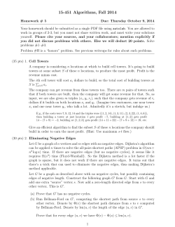
4. Consider a path between two vertices s and t in an undirected weighted graph G. The
bottleneck length of this path is the maximum weight of any edge in the path. The bottleneck
distance between s and t is the minimum bottleneck length of any path from s to t. (If
there are no paths from s to t, the bottleneck distance between s and t is ∞.)
1
11
6
4
5
10
s
t
3
2
7
9
8
12
The bottleneck distance between s and t is 5.
Describe an algorithm to compute the bottleneck distance between every pair of vertices
in an arbitrary undirected weighted graph. Assume that no two edges have the same
weight.
5. (a) Describe and analyze an algorithm to compute the maximum-weight spanning tree of
a given edge-weighted graph.
(b) A feedback edge set of an undirected graph G is a subset F of the edges such that every
cycle in G contains at least one edge in F . In other words, removing every edge in F
makes the graph G acyclic. Describe and analyze a fast algorithm to compute the
minimum weight feedback edge set of of a given edge-weighted graph.
6. Suppose we are given both an undirected graph G with weighted edges and a minimum
spanning tree T of G.
(a) Describe an algorithm to update the minimum spanning tree when the weight of a
single edge e is decreased.
(b) Describe an algorithm to update the minimum spanning tree when the weight of a
single edge e is increased.
In both cases, the input to your algorithm is the edge e and its new weight; your algorithms
should modify T so that it is still a minimum spanning tree. [Hint: Consider the cases e ∈ T
and e 6∈ T separately.]
7. (a) Describe and analyze and algorithm to find the second smallest spanning tree of a
given graph G, that is, the spanning tree of G with smallest total weight except for
the minimum spanning tree.
? (b)
Describe and analyze an efficient algorithm to compute, given a weighted undirected
graph G and an integer k, the k spanning trees of G with smallest weight.
9
Algorithms
Lecture 20: Minimum Spanning Trees [Fa’14]
8. We say that a graph G = (V, E) is dense if E = Θ(V 2 ). Describe a modification of Jarník’s
minimum-spanning tree algorithm that runs in O(V 2 ) time (independent of E) when the
input graph is dense, using only simple data structures (and in particular, without using a
Fibonacci heap).
9. (a) Prove that the minimum spanning tree of a graph is also a spanning tree whose
maximum-weight edge is minimal.
? (b)
Describe an algorithm to compute a spanning tree whose maximum-weight edge is
minimal, in O(V + E) time. [Hint: Start by computing the median of the edge weights.]
10. Consider the following variant of Borvka’s algorithm. Instead of counting and labeling
components of F to find safe edges, we use a standard disjoint set data structure. Each
component of F is represented by an up-tree; each vertex v stores a pointer parent(v) to
its parent in the up-tree containing v. Each leader vertex v¯ also maintains an edge safe(¯
v ),
which is (eventually) the lightest edge with one endpoint in v¯’s component of F .
Borvka(V, E):
F =∅
for each vertex v ∈ V
parent(v) ← v
while FindSafeEdges(V, E)
AddSafeEdges(V, E, F )
return F
FindSafeEdges(V, E):
for each vertex v ∈ V
safe(v) ← Null
found ← False
for each edge uv ∈ E
¯ ← Find(u); v¯ ← Find(v)
u
¯ 6= v¯
if u
if w(uv) < w(safe(¯
u))
safe(¯
u) ← uv
if w(uv) < w(safe(¯
v ))
safe(¯
v ) ← uv
found ← True
return done
AddSafeEdges(V, E, F ):
for each vertex v ∈ V
if safe(v) 6= Null
x y ← safe(v)
if Find(x) 6= Find( y)
Union(x, y)
add x y to F
Prove that if Find uses path compression, then each call to FindSafeEdges and
AddSafeEdges requires only O(V + E) time. [Hint: It doesn’t matter how Union is
implemented! What is the depth of the up-trees when FindSafeEdges ends?]
11. Minimum-spanning tree algorithms are often formulated using an operation called edge
contraction. To contract the edge uv, we insert a new node, redirect any edge incident to u
or v (except uv) to this new node, and then delete u and v. After contraction, there may
be multiple parallel edges between the new node and other nodes in the graph; we remove
all but the lightest edge between any two nodes.
10
Algorithms
Lecture 20: Minimum Spanning Trees [Fa’14]
8
5
8
10
30
12
14
4
5
8
3
3
2
18
5
10
3
16
30
18
12
16
30
12
14
4
26
4
16
14
26
26
Contracting an edge and removing redundant parallel edges.
The three classical minimum-spanning tree algorithms can be expressed cleanly in terms of
contraction as follows. All three algorithms start by making a clean copy G 0 of the input
graph G and then repeatedly contract safe edges in G; the minimum spanning tree consists
of the contracted edges.
• Borvka: Mark the lightest edge leaving each vertex, contract all marked edges, and
recurse.
• Jarník: Repeatedly contract the lightest edge incident to some fixed root vertex.
• Kruskal: Repeatedly contract the lightest edge in the graph.
(a) Describe an algorithm to execute a single pass of Borvka’s contraction algorithm in
O(V + E) time. The input graph is represented in an adjacency list.
(b) Consider an algorithm that first performs k passes of Borvka’s contraction algorithm,
and then runs Jarník’s algorithm (with a Fibonacci heap) on the resulting contracted
graph.
i. What is the running time of this hybrid algorithm, as a function of V , E, and k?
ii. For which value of k is this running time minimized? What is the resulting
running time?
(c) Call a family of graphs nice if it has the following properties:
• A nice graph with n vertices has only O(n) edges.
• Contracting an edge of a nice graph yields another nice graph.
For example, graphs that can be drawn in the plane without crossing edges are nice;
Euler’s formula implies that any planar graph with n vertices has at most 3n − 6 edges.
Prove that Borüvka’s contraction algorithm computes the minimum spanning tree of
any nice n-vertex graph in O(n) time.
© Copyright 2014 Jeff Erickson.
This work is licensed under a Creative Commons License (http://creativecommons.org/licenses/by-nc-sa/4.0/).
Free distribution is strongly encouraged; commercial distribution is expressly forbidden.
See http://www.cs.uiuc.edu/~jeffe/teaching/algorithms for the most recent revision.
11