
Competition among Exchanges∗
Competition among Exchanges∗
Markus Baldauf
Joshua Mollner
Version: January 8, 2015
Please find the latest version of the paper at
http://stanford.edu/~baldauf/JMP_baldauf.pdf.
Abstract
This paper applies an econometric model of imperfect competition to equity trading
with competing exchanges. Stock of the same company is traded on multiple venues
today. This development was driven by regulations, aimed at benefiting investors by
fostering competition among exchanges. However, the welfare consequences of increased
exchange competition are theoretically ambiguous. While competition does place downward pressure on the bid-ask spread, this force may be outweighed by increased adverse
selection that stems from additional arbitrage opportunities. We investigate this ambiguity empirically by estimating key parameters of the model using detailed trading data
from Australia. The benefits of increased competition are outweighed by the costs of
multi-venue arbitrage. Compared to the prevailing duopoly, we predict that the counterfactual spread under a monopoly would be 23 percent lower. Further, market design
variations on the continuous limit order book would eliminate profits from cross-venue arbitrage strategies and reduce the spread by 51 percent. Finally, eliminating off-exchange
trades, so-called dark trading, would reduce the spread by 11 percent.
∗
We are indebted to our advisors Timothy Bresnahan, Gabriel Carroll, Jonathan Levin, Monika Piazzesi,
and Paul Milgrom. We would also like to thank Lanier Benkard, Alan Crawford, Darrell Duffie, Liran Einav,
Duncan Gilchrist, Terrence Hendershott, Peter Reiss, Alvin Roth, and seminar participants at Stanford, as
well as various industry experts for valuable comments. This work used the Extreme Science and Engineering
Discovery Environment (XSEDE), which is supported by National Science Foundation grant number OCI1053575. We acknowledge financial support by the Kohlhagen Fellowship Fund and the Kapnick Fellowship
Program through grants to the Stanford Institute for Economic Policy Research. Contact details: Stanford
University Economics Department. 579 Serra Mall, Stanford, CA 94305, [email protected] (Baldauf) and
[email protected] (Mollner).
1
1
Introduction
Over the past decade, equity markets have become increasingly fragmented. In December
2004, the US had 14 venues for trading equities, and NYSE handled 79.5 percent of trade
volume in NYSE-listed stocks. By December 2013, the number of active trading venues had
risen to 55, and the NYSE share of trading in NYSE-listed stocks had fallen to 22.5 percent
(NYSE Euronext, 2014; BATS Global Markets, 2014).1 Similar changes have happened in
Australia, Europe, and Japan. We present and estimate a model of imperfect competition
to investigate the effect of this development. This proliferation of trading venues and the
accompanying dispersion of trades were actively encouraged by the Securities and Exchange
Commission, in which the regulator argued that “vigorous competition among markets promotes more efficient and innovative trading services” (SEC, 2005, Reg NMS).
The intuition that competition among exchanges benefits investors should resonate with
any economist. However, in public equity markets there may be drawback to spreading out
trade across markets: dispersion may create opportunities for fast traders to engage in highfrequency arbitrage across venues. In this paper, we consider a model in which markets
compete for traders and there is potential for arbitrage trading as in Budish, Cramton, and
Shim (2013, BCS), who focus on a single market. Traders are either regular investors with an
intrinsic motive to buy or sell, or professionals who trade for profit in two ways. They either
provide liquidity, by offering to intermediate between investors, or they engage in arbitrage,
by exploiting differences between quoted prices and the fundamental asset value.
With more exchanges, venues charge lower fees to attract traders. However, traders who
provide liquidity face more difficult conditions, because any news about fundamentals enables
an arbitrageur to trade against more active quotes in aggregate before they can be adjusted
or withdrawn, for a constant amount of regular investor trades against whom to offset these
losses. We capture this trade-off in a parsimonious model of continuous time limit order book
1
The term “trading venue” encompasses (i) formal exchanges, (ii) alternative trading systems (ATSs), which
include dark pools and electronic crossing networks, and (iii) national securities associations (i.e. NASDAQ
before it became an exchange). The number of venues is estimated based on figures by Mostowfi (2014, TABB
Group), SEC and FINRA (2014).
2
trading, which extends the high-frequency trading model of BCS. We show that depending
on factors such as the extent of the private transaction motives of investors, their arrival rate
to the market, and their willingness to substitute among different exchanges, the introduction
of new exchanges can either increase or decrease the spreads faced by regular investors.
We then perform an empirical analysis of how an increase in exchange competition affects
trading. Our data comes from Australia whose market environment consists of only two
formal exchanges but is otherwise very similar to that of the United States. We use data
from the first half of 2014 to estimate the parameters of our model. We find that investors
are worse off under the prevailing duopoly than they would be under a monopoly exchange.
In section 2 we develop a model of exchange competition, and we present the equilibrium
in section 3. Our baseline model features a single asset whose shares are traded in continuous
limit order books on multiple exchanges. The fundamental asset value is public information
and evolves stochastically as a random walk. There are three types of strategic decision makers: exchanges, high-frequency traders, and investors. Exchanges operate trading platforms
and earn profits from transaction fees. High-frequency traders may trade for profit by speculating or by facilitating transactions with other traders. Investors arrive stochastically with
private trading motives and are differentiated along two dimensions. First, they differ by the
strength of their private need to transact. Second, they differ in terms of their willingness
or ability to substitute among venues for a given price difference. This may be thought of as
the result of an agency problem between an investor and a broker who routes orders to an
exchange. In practice, a broker may not always route a client’s order to the best venue, either
because of the relationship between venue and broker, or because of incomplete information
about prices at every instant.
Two forces give rise to a bid-ask spread in this model: (i) the market power of exchanges,
and (ii) adverse selection stemming from a race to react to information. Regarding the second
force, although information is publicly observable, adverse selection arises from a liquidity
provider’s inability to cancel mispriced quotes. A change in the number of venues affects the
magnitude of each of these two forces. There are consequently two opposing channels through
3
which a change in the number of exchanges affects the equilibrium bid-ask spread. First, an
increase in the number of exchanges reduces the bid-ask spread through the “competition
channel.” Intuitively, exchanges have less market power when there are more exchanges.
They consequently charge lower transaction fees, which are passed on as lower spreads, other
things being equal. Second, an increase in the number of exchanges raises the spread through
the “exposure channel.” Because investor demand is indivisible, one share must be offered
at the bid and the ask at each exchange. With more exchanges present, the aggregate book
is therefore deeper.2 More aggregate depth, in turn, implies that for any given change in
fundamentals there are more mispriced quotes and, thus, more arbitrage opportunities. This
creates larger losses for liquidity providers, who in turn demand a higher spread, other things
being equal. Theory is silent on whether lower spreads will prevail under a monopoly or an
oligopoly, since either the competition channel or the exposure channel may dominate.
In section 4 we investigate empirically the magnitudes of these two forces. We analyze
order-level data pertaining to the Australian exchange-traded fund SPDR S&P/ASX 200
FUND (STW). Our sample comprises 76 trading days from the first half of 2014. Australia
provides a unique opportunity for testing hypotheses relating to competition among exchanges
because a large fraction of the equity trading universe is observable. First, there are only two
formal exchanges active in Australia, the Australian Securities Exchange (ASX) and Chi-X
Australia (Chi-X), on both of which we have data. Second, for the security that we study
there are no overlaps in trading hours with exchanges other than ASX and Chi-X. Thus, our
dataset contains all actions that affect lit equity trading. Third, “dark” trades, or equity
trades that do not fall in the category of lit trading, occur less frequently in Australia than
in the United States.3 This is important since dark trades are not observed by us. We then
use the STW data to estimate the parameters of our model.
In section 5 we evaluate a number of counterfactuals of the estimated model. In the first
2
That aggregate depth is increasing in the number of trading venues is a stylized fact that has been
documented in the empirical literature (Boehmer and Boehmer, 2003; Fink, Fink, and Weston, 2006; Foucault
and Menkveld, 2008; Aitken, Chen, and Foley, 2013).
3
In August 2014 dark trades accounted for 37.0 percent of the shares traded in the US compared to 21.3
percent of shares traded in Australia (BATS Global Markets, 2014; Fidessa, 2014).
4
class of counterfactual analyses, we compare the currently observed outcome under a duopoly
to what would prevail under a monopoly. We find that the monopoly spread would be 23
percent lower than the duopoly spread of 2.9 cents. Thus, the exposure channel dominates
the competition channel in the case of STW.
Next, we use the estimated model to study an alternative trading mechanism aimed at
mitigating the adverse selection that stems from the race to act on public information. We
propose a mechanism, which we call selective delay, a modification of the continuous limit
order book whereby a small delay is added to the the times at which certain order types are
processed. This mechanism protects the liquidity provider by allowing him to cancel stale
quotes before they are exploited. This reduces the equilibrium spread by eliminating the
adverse selection component, leaving only the market power component. Using the estimates
to quantify this reduction, we find that with two exchanges the counterfactual spread under
a selective delay duopoly is 51 percent lower than the spread under the limit order book
status quo. In an appendix we contrast selective delay to frequent batch auctions, a familiar
design approach that has gained recent popularity (Madhavan, 1992; Budish, Cramton, and
Shim, 2013). In our setting, the two designs achieve equivalent outcomes, yet selective delay
is easier to implement.
Finally, we use the estimated model to inform our understanding of the effects of dark
trading. Such trades occur outside of the scope of an order book of an exchange, and they
consist of internalization of retail order flow by brokers, trading in dark pools, and overthe-counter trades. Dark trades have increased in prevalence over the past decade and their
effects on formal exchanges are currently being debated. We study the counterfactual of
eliminating dark trading in Australia, which currently constitutes 21 percent of volume traded
there. Within the model this corresponds to a commensurate increase in the arrival rate of
investors at the exchanges. This reduces adverse selection and lowers the equilibrium spreads
on exchanges by 11 percent.
5
1.1
Related Literature
This paper contributes to the literature on competition between platforms in financial markets. Early contributions to this literature have identified several mechanisms through which
market fragmentation can decrease welfare: with many venues price variance on a market
may increase (Economides and Siow, 1988); price impact of a single trader may be larger
(Pagano, 1989); a coordination failure of buyers meeting sellers may arise (Mendelson, 1987);
or adverse selection may increase since an informed trader has more opportunities to camouflage (Chowdhry and Nanda, 1991). Typically, in these earlier contributions multiple markets
are modeled as operating in isolation without cross-venue arbitrage. On the other hand, a
defining characteristic of trading today is that markets are electronically linked and information flows quickly from one venue to another. In this paper we show that even if traders are
informed about all markets, the welfare consequences of competition among exchanges are
ambiguous.
More recent theory papers tend to associate fragmentation with welfare increases through
the following mechanisms: lower trading fees (Colliard and Foucault, 2012); and greater product differentiation, which benefits heterogeneous investors (Pagnotta and Philippon, 2013).
In this paper we embed an exchange oligopoly in an equilibrium model of continuous time
trading with hetereogeneous agents. We formalize a new channel of how fragmentation can
increase the risk of liquidity provision, and we show its empirical significance.
Our model of trading is connected to the branch of the literature that has focused on
adverse selection. Early models of this include Copeland and Galai (1983) and Glosten and
Milgrom (1985). Most recently, Budish, Cramton, and Shim (2013) have demonstrated that
similar forces arise in limit order books even when information is public. While our model
builds upon their framework, we allow for imperfect competition among exchanges, which
provides an additional source of a bid-ask spread.
Finally, this paper is related to a rich empirical literature on fragmentation of financial
markets. Typically, these papers either evaluate cross-sectional variation of fragmentation
(O’Hara and Ye, 2011; Gajewski and Gresse, 2007; Porter and Thatcher, 1998) or panel
6
variation of fragmentation (K¨
orber, Linton, and Vogt, 2013; Degryse, de Jong, and van Kervel,
2014), or they study a change in market structure, such as entry by an exchange (Menkveld,
2013, 2014; Aitken, Chen, and Foley, 2013), the expiration of warrants (Amihud, Lauterbach,
and Mendelson, 2003), or changes in the trading rules (Davis and Lightfoot, 1998). There is
little consensus among these papers as to the effects of fragmentation. A common difficulty
with all these approaches is clean identification. Specifically, the addition of a new exchange
may be disruptive to the market, may occur over a long time horizon of months or more, and
the market may take some time to converge to the new long run equilibrium. Also, whether a
security is traded on multiple venues is typically not randomly assigned but may be affected
by its market capitalization or other characteristics. Our empirical approach is different. We
instead estimate key parameters of a model of demand for liquidity. This approach does not
suffer from the difficulties of identification that are prevalent in this literature, and it allows
us to evaluate counterfactuals about market structure.
2
Model
The building block for our analysis is the demand system that governs trade flow of investors
across exchanges. We first set out the trading environment and then we introduce the decision
makers.
2.1
Trading Environment
Asset.
There is a single asset whose fundamental value at time t is vt . Shares of that asset
are traded at one or more exchanges. Trading begins at t = 0, at which point the fundamental
value v0 is public information. Trading ends at t = T . During the interval [0, T ], vt evolves
as a compound Poisson jump process with arrival rate λj ∈ R+ . Positive and negative jumps
occur with equal probability and all have a size of γ ∈ R+ .
For example, the asset may be a company, and the times {0, T } may represent the dates
of release of quarterly earnings reports. Jumps in vt may represent realizations of profits,
7
which are not made public until after the release of the next quarterly earnings report.
Limit order book (the “book”). The status quo trading environment in the model is a
limit order book.4 At any point in time, the book is a collection of active limit orders.
In what follows, we refer to four types of orders. A limit order consists of (i) the number
of shares desired to transact, positive if the trader wishes to sell or negative if the trader
wishes to buy, (ii) a price, and (iii) a time until when the order stays in force. Limit orders,
unless otherwise specified, are assumed to be “good ‘til cancelled.” An immediate or cancel
order is a limit order with a time in force of zero. A market order may be thought of as an
immediate or cancel order with a limit price of positive or negative infinity. A cancellation
order instructs the exchange to remove an active order from the book.
Orders are processed sequentially, in the order they are received. In the event that two
orders are received simultaneously, ties are broken at random. Incoming limit orders are
processed as follows. First, it is checked whether the incoming order makes possible trade
with any orders residing in the book. If so, then the order leads to an execution at the price
of the order in the book. If no match is found then the order is added to the book.
The bid is the highest price at which there exists an offer to buy. The ask is the lowest
price at which there exists an offer to sell. The mid price is the average of the bid and ask.
The spread is the difference between the bid and ask. The spread is a measure of transaction
costs, and in this model captures the welfare of ordinary traders.
2.2
Decision Makers
There are two types of traders: high-frequency traders and investors. In addition, exchanges
are also strategic decision makers. All agents are risk-neutral, do not discount the future,
and maximize profits.
Exchanges.
There are X exchanges, each of which allows shares of the asset to be traded
throughout the interval [0, T ]. In the status quo, each exchange is organized as a separate
4
See appendix C for a more detailed description of the order book design.
8
book. We later consider alternative trading environments. Exchanges are horizontally differentiated.5 Formally, we model this by assuming that exchange x is located at some point
lx on a circle with unit length, as in Salop (1979).6 We do not model the entry game of
exchanges but solve for the equilibrium under a fixed number.
Exchange x sets a per-transaction fee, τx , which is collected from the passive party of
each trade that occurs on that exchange. We assume that trading fees are chosen once and
for all before trading commences at time zero.
Investors.
Investors arrive at a Poisson rate λi with a desire to transact one share of the
˜ The first component, ˜l, is drawn indesecurity. Investors have two dimensional types (˜l, θ).
pendently and identically distributed from U [0, 1] and denotes a position on the aforemen˜ is drawn independently and identically distributed
tioned circle. The second component, θ,
from U [−θ, θ] and denotes a private benefit from trading a share of the asset.7
An investor who arrives at time t chooses an exchange x ∈ {1, . . . , X} and a quantity to
transact y ∈ {−1, 0, 1} to maximize
⎧
⎪
⎪
⎪
vt + θ˜ − ax,t − α ⋅ d(˜l, lx )
⎪
⎪
⎪
⎪
⎪
⎪
˜ ˜l) = ⎪
⎨bx,t − vt − θ˜ − α ⋅ d(˜l, lx )
u(y, x∣θ,
⎪
⎪
⎪
⎪
⎪
⎪
⎪
⎪
⎪
−α ⋅ d(˜l, lx )
⎪
⎩
if y = 1
if y = −1
if y = 0
where bx,t (ax,t ) denotes the relevant bid (ask) price for selling (buying) one share at exchange
x at time t. The function d yields the distance between two points on the unit circle.8
Moreover, α parametrizes the relative importance of the price component and the “travel
5
In practice, exchanges may differ regarding the infrastructure that they provide. Furthermore, a broker
may have an ownership stake in an exchange.
6
In the duopoly we assume that the two exchanges are not located on the same point. In the oligopoly case
we assume that all exchanges are located equidistantly, i.e. that they follow maximum differentiation. Under
this assumption, the existence of a Nash equilibrium of the location game, which we do not model explicitly,
is well-understood (Anderson, De Palma, and Thisse, 1992, Proposition 6.6).
7
This private benefit may be thought of as coming from, for example, an idiosyncratic desire to hedge,
save, or borrow. It is through this private benefit that gains from trade are realized. These traders play the
role of the liquidity traders of Glosten and Milgrom (1985) or the noise traders of Kyle (1985).
8
Formally, d(l1 , l2 ) = min(∣l1 − l2 ∣, 1 − ∣l1 − l2 ∣).
9
cost” or the horizontal differentiation component.
˜ ˜l). First, it may be a literal representation
There are two interpretations of u(y, x∣θ,
of the utility of an investor, so that travel costs directly enter the preferences of investors.
Second, travel costs may not directly enter the preferences of investors. In this interpretation,
investors do not always act to maximize their utility. This could be thought of as the result
of an unmodeled agency problem, whereby the location parameter ˜l is actually a property of
the investor’s broker, which influences the broker’s actions in such a way that they are not
always in his client’s best interest.9 An investor who arrives at time t may act only at time
t and is restricted to immediate or cancel orders.10
High-frequency traders. There is an infinite number of high-frequency traders, each
with the objective of maximizing trading profits.11 They are risk neutral and there is no
discounting. The action space of a high-frequency trader at any time t includes whether to
submit any limit orders or cancellations.
2.3
Assumptions
We use three assumptions in deriving the results that follow. These assumptions place restrictions on the parameter space, which guarantee that the market does not break down and
that the equilibrium features trading based on changes in fundamentals.
Define
⎧
⎪
λj
⎪
⎪
θ (1 + )
⎪
⎪
⎪
λi √
σ≡⎨
⎪
λj
2
4
⎪
⎪
2 + α2
⎪
θ
+
α
−
θ
−
4αθ
⎪
⎪
X
X2
λi
⎩
9
if X = 1
if X ≥ 2
This agency problem may stem from, for example, so-called “maker-taker” pricing. This refers to the
fact that some exchanges may in practice provide rebates to the broker on a certain side of a trade. Brokers
may then deviate from their obligation to obtain best prices for a client and instead focus on collecting these
rebates. Battalio, Corwin, and Jennings (2013) document empirical evidence of this occurring in practice.
10
The restriction of investors to immediate or cancel orders prevents them from providing liquidity and is
quite standard in the literature, for example as in Glosten and Milgrom (1985) and Budish, Cramton, and
Shim (2013).
11
In practice, the number of high-frequency traders is quite large. For example, Baron, Brogaard, and
Kirilenko (2012) identify 65 separate high-frequency trading firms that actively trade the E-mini S&P contract
in August 2010. Furthermore, since each firm may employ several different high-frequency trading algorithms,
the effective number of competitors may be even higher.
10
Assumption 1 (investor participation). σ ≤ 2θ.
Assumption 2 (scalper participation). σ ≤ 2γ.
Assumption 3 (exchange participation). λi (1 −
1σ σ
σ
) − λj X (γ − ) ≥ 0.
θ2 2
2
Assumption 1 ensures that the spread is not so large that it crowds out all trades by
investors whose private transaction motives are bounded by θ. If this assumption were
violated, then the market would shut down due to adverse selection, since only informed
trades would occur. Therefore, this is a technical assumption and not likely to bind in
practice.
Assumption 2 ensures that trades following a change in the pricing benchmark occur in
equilibrium. If this assumption were violated, then the liquidity provider would not face
adverse selection risk. The risk of trading at a loss with an informed party is a pertinent
feature of financial markets, which provides a motivation for this assumption.
Assumption 3 ensures that exchanges earn nonnegative equilibrium profits, and therefore
have no incentive to shut down.
3
Limit Order Book Equilibrium
In this section, we study the case in which each exchange is organized as a limit order book.
We describe Nash equilibrium trading behavior in this environment, characterize equilibrium
outcomes, and we discuss how these outcomes depend on the parameters of the model.
3.1
Equilibrium
In this section, we demonstrate the existence of equilibria in which various numbers of exchanges each operate a separate order book. The equilibrium depends upon the number of
exchanges in the economy. Theorem 1 characterizes the equilibrium spread for the case of a
monopoly, and theorem 2 does the same for an oligopoly.
11
Theorem 1 (Monopoly). With a single exchange (X = 1), under assumptions 1, 2 and 3,
there exists a Nash equilibrium of the limit order book design with spread
s∗LOB = θ (1 +
λj
).
λi
Theorem 2 (Oligopoly). With multiple exchanges (X ≥ 2), under assumptions 1, 2 and 3,
there exists a Nash equilibrium of the limit order book design with spread
√
s∗LOB
(Xθ + 2α)λi −
=
(X 2 θ2 + 4α2 ) λ2i − 4X 2 αλj λi θ
.
Xλi
All proofs are deferred to appendix B. While complete descriptions of the strategies used in
these equilibria are provided in the proofs of these results, we provide an intuitive description
of these strategies here.
Investors submit orders to buy or sell in correspondence with their types. Upon arrival
they choose an exchange as well as whether to buy, sell, or hold. Separate high-frequency
traders play the roles of “liquidity provider” at each exchange. Each liquidity provider maintains quotes of one unit at the bid and one unit at the ask. They set mid prices equal to
the fundamental value of the asset, and they set spreads to satisfy a zero-profit condition.
The remaining high-frequency traders play the role of “stale-quote scalpers,” attempting to
trade whenever a jump in the value of the asset generates a mispricing in the quotes of the
liquidity provider.12 Formally, the liquidity provider ties in a race to react on information
with an infinite number of scalpers, which the scalpers as a sector always win.13 Finally, each
exchange sets a transaction fee to maximize profits, taking into account the behavior of the
traders and, in the case of oligopoly, competition from other exchanges.
As in BCS, free entry into high-frequency trading leads us to focus on equilibria in which
12
BCS refer to these agents as “snipers.” We depart from their terminology in order to reflect more closely
the language used by industry participants.
13
This can be thought of the limit of a process where agents face random latency when communicating with
the exchange. Provided that the liquidity provider loses the race to adjust quotes at least some of the time,
then this leads to some amount of loss-making trades from the perspective of the liquidity provider.
12
the liquidity provider earns zero profits in expectation.14 At any instant, one of two things
may affect the profits of a liquidity provider: the value of the asset may jump or an investor
may arrive. The arrival rate of jumps is λj . Conditional on a jump occurring, the liquidity
provider at exchange x will lose γ−sx /2 to the stale-quote scalper and must pay the transaction
fee τx to the exchange. Note that assumption 2 guarantees that scalpers make nonnegative
profits in aggregate. On the other hand, the arrival rate of investors is λi . In the case
of an oligopoly, an exchange x is the preferred exchange of an investor with probability
(s−x − sx ) /(2α)+1/X when the spreads are sx on exchange x and s−x on the other exchanges.
In the case of a monopoly, the monopolist exchange is always the preferred exchange of an
investor. Conditional on exchange x being the preferred exchange of an investor, that investor
trades with probability 1−sx /(2θ). Note that by assumption 1 this probability is nonnegative
at the equilibrium spread. Conditional on the investor trading, the liquidity provider earns
the half-spread, sx /2, and must pay the transaction fee τx to the exchange. The zero profit
condition of a liquidity provider is then
λi (1 −
sx
1 sx sx
) ( − τx ) − λj (γ −
+ τx ) = 0
θ 2
2
2
in the case of a monopoly, and is
λi [
1 s−x sx
1
1 sx sx
sx
(
− ) + ] (1 −
) ( − τx ) − λj (γ −
+ τx ) = 0
α 2
2
X
θ 2
2
2
in the case of an oligopoly. Conditional on exchange x setting the transaction fee τx , the
liquidity provider on exchange x sets a spread sx to satisfy the appropriate zero profit condition. Exchange x takes this behavior as given, and sets a transaction fee τx to maximize
its profits, which are the product of τx and the volume traded. The resulting equilibrium
14
GETCO (KCG since its merger with Knight Capital Group in 2013) is a representative, significant global
player in high-frequency trading and in market making of equities. Its 2013 Form S-4 filing with the SEC
reveals that its net income decreased by 41.9 percent from USD 232.0 in 2007 to USD 167.2 million in 2011
(KCG, 2013, p. 31). For Q2 2013, its market making division even posted a loss of USD 1.9 million compared
to a profit of 9.3 million in the previous year (KCG, 2013, Exhibit 99.2, p. 8). To the extent that excessive
profits accrued to liquidity providers during the previous decade, they were short-lived.
13
spread is as described in theorem 1 for the case of a monopoly. For the case of an oligopoly,
we focus on symmetric equilibria, in which the same spread prevails at each exchange. The
resulting equilibrium spread is as described in theorem 2.
Two forces give rise to an equilibrium spread in our model, both of which are illustrated
by the expression for the monopoly spread given in theorem 1. First, since a monopolist sets
prices according to own-price elasticity of demand, the spread is a function of the investor’s
private willingness to transact, θ. Indeed in the absence of adverse selection (i.e. with
λj = 0), the pricing equation follows the classic Lerner condition. Second, the relative flow of
information to investor arrivals, λj /λi , governs the extent of adverse selection that a liquidity
provider faces.
3.2
The Effect of Exchange Competition
A key insight formalized by this model is that the welfare consequences of the number of
exchanges are ambiguous. The ambiguity is caused by two opposing channels. On one hand,
the addition of another exchange may reduce spreads through the “competition channel.”
Intuitively, exchanges have less market power when they have more competitors and must
reduce their transaction fees to retain investors. Lower fees are passed on as lower spreads.
However, the addition of another exchange may raise spreads through the “exposure channel.”
Intuitively, more shares are quoted in aggregate. Therefore, whenever the fundamental value
of the asset moves away from the current posted prices, more shares are exposed to that
mispricing, which creates larger losses for liquidity providers. Liquidity provision therefore
becomes more risky and induces higher spreads in response.
The ambiguity may be illustrated by two limiting cases of the model. First, consider
the limiting case as α diverges to infinity, which is to say that investors do not condition
their choice of exchange on the price difference. In that case, the expression for the oligopoly
spread converges to s∗LOB = θ (1 + Xλj /λi ) . Thus, every additional exchange raises the spread
by θλj /λi . The reason is that if investors do not respond to prices, then multiple exchanges
are a collection of isolated monopolists. Yet scalpers possess more opportunities to trade on
14
a given piece of information, which increases adverse selection. Intuitively, the competition
channel is shut down, so that the exposure channel dominates.
Second, consider the case in which λj = 0, which is to say that the fundamental asset value
√
is constant. In that case, the monopoly spread is θ, and the duopoly spread is θ+α− θ2 + α2 .
Thus, the monopoly spread exceeds the duopoly spread.15 The reason is that adverse selection
does not increase with the number of exchanges, as with a constant asset value there is no
adverse selection. Yet price competition is intensified, resulting in smaller transaction fees and
hence smaller spreads. Intuitively, the exposure channel is shut down, so that the competition
channel dominates.
3.3
Comparative Statics
In this section we use the characterization of equilibrium outcomes from the previous section
to study how these outcomes vary with respect to the primitives: α, the willingness of
investors to substitute between exchanges, θ, the extent of their private transaction motive,
λi , their arrival rate, and λj , the arrival rate of information.
Theorem 3 (Comparative Statics). Within the set of parameters that satisfy assumptions
1, 2 and 3, the equilibrium spread of the limit order book design is
(i) nonincreasing in λi and
(ii) nondecreasing in λj , α, and θ.
The parameter α determines travel costs and governs the cross-price elasticity of investors.
It therefore determines the magnitude of the “competition channel.” When α is large, travel
costs are high, which mutes price competition and raises spreads. On the other hand, when
α is small, price competition is strong and spreads are lower.
The intuition for the comparative statics with respect to the arrivals of investors and
information, i.e. λi and λj , can be understood through the liquidity provider’s problem.
15
Furthermore, the equilibrium spread is also decreasing
in the number of exchanges within the oligopoly
√
2 2
2
case. With λj = 0, the oligopoly spread is θ + 2α− θ XX +4α , which is decreasing in X.
15
If investors arrive more frequently (increase in λi ), then the liquidity provider faces less
adverse selection, since she trades with relatively more investors and relatively fewer stalequote scalpers. She therefore demands a smaller spread. On the other hand, if trades based
on changes in the fundamental value occur more frequently (increase in λj ), then she faces
more adverse selection, since she trades with relatively fewer investors and relatively more
stale-quote scalpers. She therefore demands a larger spread.
The parameter θ governs the own-price elasticity of investor demand. When θ is large,
investors are quite inelastic. Exchanges can therefore afford to charge larger transaction fees,
which induces larger spreads. On the other hand, when θ is small, investors are quite elastic.
Exchanges must therefore charge smaller transaction fees, which are passed on as smaller
spreads.
3.4
Welfare of Investors, Traders, and Exchanges
In this section we present the functions that measure the welfare of the agents in the model.
We use them in section 5 to compare and evaluate counterfactuals of the estimated model.
The gains from trade stem from the investors’ private willingness to transact. Therefore, in
the model an increase in the bid-ask spread has two welfare consequences: (i) gains from
trade are reduced since investors may not trade, and (ii) they are transfers away from the
investors who do trade.
First, we consider the utility of investors. As discussed in section 2, there are two possible
interpretations of the utility of investors, depending on whether travel costs are viewed as a
part of utility or as a reflection of an agency problem between an investor and his broker.
In the case when travel costs do enter the utility of investors, the flow utility of the investor
sector in the equilibria described in theorems 1 and 2 depends on the spread and is
1
∫
0
θ
−θ
∫
∗
2
˜ ˜l = λi [ (2θ − sLOB ) − α ] ,
˜ ˜l, s∗ ) 1 dθd
λi u(y, x∣θ,
LOB
2θ
8θ
4X
which is decreasing in s∗LOB . In the case when travel costs do not enter the utility of investors
16
but instead reflect an agency problem, the utility of investors simplifies to the previous
expression evaluated at α = 0.
Second, while each high-frequency trader earns zero profits in equilibrium, there are an
infinite number of them, and they earn positive profits as a sector. Following every jump
in the underlying asset, one high-frequency trader gets to transact against the stale quote
on each exchange. Each of these trades yields a profit of the size of the jump minus the
half-spread. The flow utility of the high-frequency trading sector in the equilibria described
in theorems 1 and 2 is
Xλj (γ −
s∗LOB
).
2
Finally, the flow utility of the exchange sector in the equilibria described in theorems 1
and 2 is given by
λi
s∗
s∗LOB (2θ − s∗LOB )
− Xλj (γ − LOB ) .
4θ
2
Summing the above expressions yields the total flow utility of all agents, which is given
by
λi [
4θ2 − (s∗LOB )2
α
−
].
8θ
4X
As above, in the case when travel costs do not enter the utility of investors but instead reflect
an agency problem, the expression simplifies to the previous equation evaluated at α = 0.
From this equation it is clear that total welfare is higher under lower spreads.
4
Empirical Analysis
In this section we estimate the model using data from Australia. We proceed by describing
the industry background and then discuss the order-level data from all Australian exchanges.
Next, we introduce the empirical strategy and identification. Finally, we discuss the results
from GMM estimation.
17
4.1
Industry Background
Our empirical analysis focuses on Australia. The public equity trading landscape in Australia
is broadly similar to the United States and, in particular, has seen a comparable, albeit less
pronounced, shift toward fragmentation. In many cases the same large trading firms are active
in Australia, and they use identical trading technology as they do elsewhere. The market
participants include banks such as Citigroup, Bank of America Merrill Lynch, and Goldman
Sachs, electronic trading firms and hedge funds such as GETCO and Citadel, as well as retail
brokers such as E*trade and Interactive Brokers. Furthermore, the technical protocol that is
used by Australian exchanges is owned by Nasdaq OMX Group and is effectively the same
as that used on Nasdaq.
There are two formal exchanges currently active in Australia: the Australian Securities
Exchange (ASX) is the incumbent, and Chi-X Australia (Chi-X) is a competitor who entered
in October 2011. The share of volume traded at Chi-X amounts to 17.2 percent across all
securities during the first half of 2014.16
For reasons of measurement, Australia is a natural environment on which to focus. In
particular, data is available on almost the entire universe of trading in Australia. Of the total
volume of shares traded, 78.7 percent are “lit” and occur in the limit order books of either
ASX or Chi-X.17 Furthermore, the security we study is only traded on these two exchanges.
4.2
Data
This section documents the datasets and variables that are used for the empirical investigation. We proceed in three steps, describing (i) the raw order-level data, (ii) the reconstruction
of the limit order books in continuous time, and (iii) the construction of the analytic dataset
that is used for estimation.
16
For the security we study, the average daily Chi-X share in the first half of 2014 is 23.1 percent with an
interquartile range from 12.7 to 31.1 percent.
17
For the security we study, on average 87.3 percent of the volume was traded in the limit order books of
either ASX or Chi-X. For comparison, for a comparable security in the US, e.g. the S&P 500 ETF, trades
take place on more than 40 different venues.
18
4.2.1
Order-Level Data
The starting point of our empirical investigation is a complete record of messages that are
broadcast by ASX and Chi-X as publicly available data feeds, which market participants can
access in real time for a fee.18 These messages contain pertinent information about the state
of the limit order books at ASX and Chi-X for every listed security. Specifically, a message
is broadcast to notify market participants about every order that alters the order book.19
Messages that affect the book are new add orders, cancellations, and executions of existing
orders.
Starting from a chronological record of all messages, we isolate all messages pertaining
to the exchange-traded fund STW, which aims at replicating the Australian market index
S&P/ASX 200. In appendix D we document the details about the data and the specific
steps taken for message parsing. This security is of broad interest for two reasons. First,
STW is a highly liquid ETF that replicates a basket of 200 constituents, which account for
approximately 80 percent of Australian equity market capitalization. The current market
capitalization of the fund is AUD 2.45 billion (SPDR, 2014). Therefore, this security is
representative of a considerable part of trading in Australia. Second, the bid-ask spread of
STW is not typically constrained by the minimum tick size of 1 cent, as is the case for many
other thickly-traded securities.20
Table 1 shows the distribution of messages that affect the order books of STW at ASX and
Chi-X. Two aspects of these data merit mention. First, only a small fraction of messages are
related to executions, 1.93 percent at ASX and 0.44 percent at Chi-X. The remainder divides
almost equally in add orders or cancellations of active orders.21 Second, the order flow at the
two trading venues is similar. On a typical day, trading in STW generates 14,596 messages
at ASX compared to 14,447 messages at Chi-X. The difference between executions at the
18
These broadcasts are called “ITCH – Glimpse” and “Chi-X MD Feed” at ASX and Chi-X respectively.
There are also a number of other messages that relate to system events and the opening and closing
auctions, which we do not use for this paper.
20
During instances when the minimum tick size is binding, the first order conditions that stem from the
solution to our model, do not hold.
21
Cancelations and executions do not sum to the number of add orders due to the possibility of add and
cancel orders outside of the sampling frame between 10:30 and 16:00 on a trading day.
19
19
two venues points to a disagreement of model and reality. The equilibrium we study is fully
symmetric with regards to spreads, order flow, and trade flow. However, in reality spreads
and order flow exhibit a greater degree of symmetry than trade flow. We view our model as
a useful instrument to inform the price setting in financial markets and less well-suited to
inform trade volumes.
Table 1: Messages affecting the limit order book
message types
add
cancel
execution
total
ASX
N
%
550,151
49.60
537,736
48.48
21,384
1.93
1,109,271 100.00
Chi-X
N
%
546,460
49.77
546,660
49.79
4,878
0.44
1,097,998 100.00
Distribution of messages that affect the state of the limit order book of
SPDR S&P/ASX 200 FUND (STW). Based on ASX ITCH – Glimpse
and Chi-X MD feed data. Sample period: 10:30 – 16:00 for 76 trading
days between Feb 3, 2014 and May 30, 2014.
4.2.2
Continuous Time Limit Order Book
We then proceed to reconstruct the order books for STW at each of the two exchanges.22
Our reconstruction algorithm replicates the matching processes used by the exchanges. At
each exchange it involves the following steps. All messages are processed in chronological
order. When an add order arrives, it is added to the book at the limit price that it specifies.
In case of a cancellation, the active order in question is removed. Finally, in the event of
an execution, the affected order is removed or its quantity is adjusted.23 In appendix D we
describe the steps of constructing the analytic dataset in detail.
22
Since the book at any moment is a cumulative object based on orders that were processed on that day,
we start the reconstruction when the market opens. We later limit the dataset to messages that lie in the
10:30 – 16:00 interval. The continuous trading session for STW starts at a random point on the interval
[9:08:45, 10:09:15], when ASX calculates and announces the opening price.
23
Suppose that an active order at the ask specifies 100 shares and a buy order for 60 shares is executed
against it. Then the active order remains with an updated quantity of 40 shares.
20
4.2.3
Discretization and Variable Construction
For the estimation we discretize time into intervals of length of one second. We define
variables pertaining to the prices prevailing in an interval, as well as whether certain types
of transactions occur.
Prices.
Based on the two order books we construct a time series of bid and ask prices, from
which we also compute a time series of bid-ask spreads for each exchange. In the event of a
price change during an interval, we use the value prevailing at the beginning of that interval.
Measuring uninformed trades. Motivated by the equilibrium behavior of the traders in
the model, we define investor trades as trades that happen in isolation from others. Specifically, a trade is termed isolated when no other trade occurs within ω duration on either
exchange.24 We define the indicator
1{isolated tradet }, which evaluates to unity if an iso-
lated transaction, either to buy or sell against a standing order, occurred on ASX or Chi-X
in interval t and zero otherwise. In the baseline specification, we set ω = 1. In appendix E,
we demonstrate that our results are robust to the choice of ω.
Measuring informed trades. In the model, informed trades occur after every change in
the fundamental asset value, and against all available mispriced quotes. Motivated by this
feature of equilibrium behavior, we define an empirical measure of informed trades based on
the clustering of trades, both across venues and time.25 A trade is classified as clustered
if it occurs within ω of another trade at either ASX or Chi-X. We define the indicator
1{clustered tradet }, which evaluates to unity if a clustered trade occurred on ASX or Chi-X
in interval t and zero otherwise. As before, we set ω = 1 in the baseline specification.
24
Technically, a single marketable limit order can lead to multiple execution messages, albeit with identical
time stamps, which we count as one execution in our analysis. Specifically, if an order to buy is large enough
to trigger a trade against two or more standing limit orders to sell, then a separate execution message is
broadcast for each match. These messages (i) appear in consecutive order, and (ii) all have the same time
stamp.
25
This definition of informed and uninformed trades relies on knowledge of the distribution of other orders
arriving at all exchanges. In Baldauf and Mollner (2014b) we use a different approach. There, we use knowledge
of the identity of market participants to classify them as informed and able to react to news quickly.
21
Table 2 shows summary statistics for four variables: the indicators for isolated and clustered trades, as well as the spreads at ASX and Chi-X. For each variable we report means
and standard deviations for the full sample that comprises the trading hours from 10:30am
until 4:00pm of each of the 76 trading days in the sample. The restricted sample consists
of those seconds for which the quotes at both exchanges during an interval are identical,
which is the case 30.7 percent of the time. For those observations, there is no difference in
the implied mid prices at ASX and Chi-X. For that reason, this is the sample that is used
for estimation. An isolated trade occurs in 0.73 percent of the seconds in the full sample.
Isolated trades are slightly more frequent in the restricted sample and occur in 0.75 percent
of seconds. Clustered trades occur on average in 0.17 percent of seconds in the full and 0.15
percent of seconds in the restricted sample.
Table 2: Summary statistics
1{isolated trade}
1{clustered trade}
spreadASX
spreadCHIX
Observations
full
Mean
Std. Dev.
0.007336
0.08541
0.001737
0.04164
2.532
1.125
2.784
0.7055
1,504,724
restricted
Mean
Std. Dev.
0.00753
0.08645
0.001548
0.03931
2.917
0.6767
2.917
0.6767
461,875
An observation is one second between 10:30 and 16:00 on one of the 76
trading days in the sample. The full sample includes all such seconds. The
restricted sample includes only seconds during which both the bid and ask
prices at ASX and Chi-X are equal. 1{isolated trade} evaluates to unity for
a second during which a trade happened conditional on no other trade happening within a second on either exchange. 1{clustered trade} evaluates to
unity for seconds during which a trade happens and a second trade happens
within one second on either exchange. Spreads are measured in cents and
are evaluated at the start of an interval.
Next, we turn to the distribution of bid-ask spreads at the two exchanges. In the restricted
sample, the spread at the two exchanges is on average 2.9 cents with a standard deviation of
0.9 cents. This compares to 2.5 and 2.8 cents at ASX and Chi-X in the full sample. Standard
errors around these averages are 1.1 and 0.7 cents respectively. Figure 1 shows the joint
density plot of the spreads at ASX and at Chi-X. The unique mode is given by a symmetric
spread of three cents at both exchanges, which occurs 22.1 percent of the time. Furthermore,
22
the spreads at both exchanges are equal 36.8 percent of the time and they differ by at most
one cent in 81.5 percent of the time.
0
2
stASX
4
6
8
Figure 1: Joint density of spreads at Chi-X and ASX
0
2
4
stChi-X
6
8
[0,0.01)
[0.01,0.05)
[0.05,0.1)
[0.1,0.15)
[0.15,0.2)
[0.2,1]
An observation is one second between 10:30 and 16:00 in one of the 76 trading days in the
sample. Each cell refers to a pair (sASX , sChi-X ). Spreads are measured in AUD cents.
The shading refers to the fraction of seconds that a pair of spreads is observed in the
sample.
4.3
Empirical Strategy
In this section we show how the observed variation in the data is used to estimate our model.
The model has four parameters that require estimation.26 Three of them are primitives that
26
There is a fifth parameter, γ, the size of the jumps in the stochastic process that governs the evolution of
the asset value. However, for the policy counterfactuals that we consider, it is not necessary to estimate this
parameter.
23
govern the choice problem of investors: the willingness to substitute between exchanges, α,
the extent of the private transaction motive, θ, and the arrival rate of investors, λi . The
fourth parameter is λj , the arrival rate of jumps in the fundamental asset value.
In what follows we show that the parameters are uniquely identified by the variation in
spreads and the occurrences of isolated and clustered trades. Intuitively, the identification
argument relies on three parts. First, the arrival rate of jumps, λj , is related to our measure
of clustered trades. Second, the arrival rate of isolated trades, in conjunction with variation
in the spread, pins down λi and θ. In addition, we present reduced-form evidence about
how spreads affect the occurrence of an isolated trade in appendix F. Finally, the level of the
spread is a function of all four parameters as shown in theorem 2, and so it pins down α.
For the estimation we use the restricted sample, in which the two bid prices are equal
and the two ask prices are also equal, since it does not introduce an ambiguity about which
mid price corresponds to the fundamental asset value, vt . The demand of investors in that
case takes the form
1{isolated tradet } = λi max (0, 1 −
st
) + εt
2θ
(1)
where 1{isolated tradet } is an indicator for an isolated trade occurring in interval t on either
exchange, and st is a measure of the prevailing spread at the beginning of interval t. Furthermore, εt is an error term that is uncorrelated with st and with zero expectation. In the
model λi is the intensity of a Poisson process and the error εt captures deviations of this
random process away from its mean.
Equation (1) gives rise to two moment conditions, which identify λi and θ.
st
∂ε2t
] = E [−2εt max (0, 1 − )] = 0
∂λi
2θ
(M1)
∂ε2t
st
λi st
] = E [1{1 −
> 0}εt (− 2 )] = 0
∂θ
2θ
θ
(M2)
E[
E[
Thus, variation in the participation of investors as a function of the spread pins down their
arrival rate and the distribution of the private willingness to transact.
24
Next, the arrival rate of informed trades is given by
1{clustered tradet } = λj + νt
(2)
where 1{clustered tradet } is an indicator for a clustered trade occurring in interval t, and νt
is a zero expectation error term which implies the following moment condition. In the model,
jumps follow a Poisson process with intensity λj and the error νt captures deviations of this
random process away from its mean.
E [νt ] = 0
(M3)
Finally, the expression for the spread under a duopoly gives rise to
√
st = θ + α −
θ2 + α2 − 4θα
λj
+ ηt
λi
(3)
where ηt is zero expectation error term that is uncorrelated from other error terms. The final
moment condition is thus
E [ηt ] = 0
(M4)
Note that the model does not suggest a reason for why the equation for the spread should
contain an error term. However, in the data, the spreads are not constant, yet are most of the
time either 2 or 3 cents. There are a number of reasons that can explain short-term deviations
from this long run pricing equation. First, we have assumed that the parameters of the model
are constant over time. While this seems accurate as a first approximation, small deviations
may arise in practice, which would give rise to different values of the spread. For example,
days on which macroeconomic news announcements are expected would be associated with
larger values of λj and γ.27 Second, in the model it is assumed that all agents are risk-neutral.
27
On such days liquidity providers would charge a larger spread. We show how liquidity providers change
their behavior following unanticipated news in Baldauf and Mollner (2014b). There, we focus on a few minutes
25
In practice, it is likely that high-frequency traders face constraints on their inventory and
may therefore adjust quoted spreads as these constraints become more or less binding.28
4.4
Parameter Estimates
We estimate the parameters by GMM, minimizing the quadratic form based on the four moment conditions (M1), (M2), (M3), and (M4). In this section we report the main estimation
results. Alternative specifications for robustness are provided in appendix E.
Table 3 contains the parameter estimates. The interpretation of the point estimates is as
follows. First, the estimate for θ of 1.6 cents points to a relatively flat schedule for the investor
demand to trade STW. This suggests that investors would divert to investment alternatives,
even for small changes in the spread. Second, the point estimate for α of 11.1 cents implies
that investors act as though the value of the difference between the best and worst trading
conditions, holding prices constant, amounts to 5.6 cents, or 1.9 times the average spread of
2.9 cents.
To illustrate the relative magnitude of the own-price and the cross-price channel of the
order flow from investors at these estimates, consider a decrease in the spread at one exchange
by 5 percent from a starting point of equal spreads at 2 cents. The overall investor flow at
that exchange increases by 9.9 percent, which can be decomposed into the own-price effect
(+9.0 percent) and the substitution effect (+0.9 percent).29
The point estimates for the arrival rates of investors and changes in the fundamental
asset value are 0.0052 and 0.0023 per second, respectively. The ratio of the arrival rates of
scalpers to investors amounts to 0.44. All estimated parameters are highly significant based
of trading in the immediate aftermath of the announcement of a terrorist attack, a more volatile time period
compared to the trading day up to the announcement. We find that, in the aftermath of the news arrival,
spreads increased compared to their levels before the event.
28
A recent example that illustrates the significance of capital constraints is the SEC’s decision to fine Latour
Trading LLC USD 16 million for violation of the net capital rule of the Exchange Act, which stipulates that
every broker-dealer must maintain a specified minimum level of net liquid assets (SEC, 2014).
29
We compare the investor trades of exchange A following a change of the spread from s to s′ while holding
the spread at exchange B constant at s as follows. Before the price change, the number of investor trades
s
). After the price change, the number of investor trades at A is given by
at A is given by λi ( 21 ) (1 − 2θ
′
′
s
λi ( 12 + s−s
) (1 − 2θ
). The change in the third term of this multiplication is what we label “own-price effect”
2α
and the change in the second term we label “substitution effect.”
26
on bootstrapped standard errors.
Table 3: GMM estimates
parameter
α
θ
λi
λj
point estimate
11.0683
1.5582
0.0052
0.0023
standard error
1.0952
0.0078
0.0002
0.0001
The point estimates are determined by minimizing the
quadratic form based on the four moment conditions that
are defined in the previous section. The sample is constructed from the continuous trading session of all trading days in our data, between 10:30-16:00. Each trading
day is divided into one second increments. Estimation is
based on the restricted sample of intervals during which
the quoted bid and ask prices at ASX and Chi-X were the
same. The estimation was performed using SNOPT (Gill,
Murray, and Saunders, 2008). Standard errors are based
on 500 bootstrap replications.
The parameter estimates, in the context of this model, place bounds on the jump size of
the fundamental value, γˆ ∈ [1.45, 1.55]. The lower bound is given by the assumption that
informed trades occur following every jump in the fundamental value (assumption 2). The
upper bound is given by the participation constraints of exchanges (assumption 3).
To evaluate whether the estimated model fits the data well we compare model predictions
to moments in the data that were not used for the estimation. First, the model makes a
clear prediction about the magnitude of the transaction fee in equilibrium, which we derive in
appendix B.1.2. Based on the parameter estimates, together with the aforementioned bounds
on γ, the predicted ratio of τ /s is in the range [0, 0.031]. Empirically, for the first half of
2014, the corresponding ratios amount to 0.052 and 0.031, for ASX and Chi-X respectively.
Our model is thus able to explain the relatively low transaction fees that are observed in this
market.
Second, the model also predicts the volatility of the fundamental asset value. For the
range of jump sizes that are implied by the model, we compute that the predicted squared
daily price movement lies in the range of [507.65, 575.65] cents squared.30 Empirically, for the
30
The assumption that a compound Poisson jump process governs the asset value evolution implies that the
27
first half of 2014, the average squared first difference in the closing prices of STW amounts
to 983.77 cents squared. The volatility of prices observed in the data is therefore larger
than that predicted by the model. This may be a result of the simplified way in which
price movements enter the model. In the model, every change in the value of the asset is
large enough that sniping is profitable. However, in practice some information may not be
sufficiently large to introduce a profitable trading opportunity. One way to incorporate this
into the model would be to allow information to accrue in two sizes: small jumps of size
γ1 and large jumps of size γ2 . If small jumps are too small to trigger any arbitrage trades,
then liquidity providers can safely update quotes without the risk of being adversely selected.
This extra degree of freedom would allow us to match the price volatility, yet would leave
the other results unchanged.
5
Counterfactuals
In this section we the estimates from section 4.4 to evaluate the following counterfactuals
within the model. First, we vary the number of exchanges in operation, while maintaining
the current limit order book design. Second, we consider an alternative market design. Third,
we evaluate the consequences of eliminating off-exchange, “dark” trades.
5.1
The Effect of Competition with Order Books
At the moment, the market structure in Australia is given by an exchange duopoly, in which
each market operates a separate order book. In our model it is theoretically ambiguous
whether competition benefits investors. The reason for that is that the competition channel
– price competition among exchanges – and the exposure channel – increased riskiness of
liquidity provision with multiple exchanges – act in opposite directions. We use the estimates
from the previous section to investigate which channel dominates in the case of STW.
The results from evaluating the expressions for the monopoly and oligopoly spreads at the
expected value of the square of the difference in prices over an interval of length δ takes the form E[(∆v)2 ] =
γ 2 λj δ, where ∆v and λj denote price difference and arrival rate of jumps during that interval.
28
estimated parameter values are reported in the first row of table 4. In the case of a monopoly
exchange, we estimate the average spread to decrease by 23 percent, from 2.92 to 2.25 cents.
The corresponding welfare change represents a four-fold increase compared to the prevailing
duopoly (table 5, row 1). Based on bootstrapped standard errors, both differences are highly
significant. Note that there does not exist a symmetric equilibrium in which three exchanges
operate that satisfies the assumptions of our model.
These findings show that the competition channel is dominated by the exposure channel.
5.2
Alternative Trading Mechanisms
A current debate among policy makers, industry participants, and researchers is concerned
with whether alternative trading mechanisms can improve upon the ubiquitous limit order
book. In this section we propose a mechanism, which we call a selective delay, in which
certain orders would be processed immediately, while other orders would be processed only
after a small delay.31 This is in contrast to a limit order book, in which orders are processed
in the order received. The benefits of a delay in processing certain orders have implicitly
been recognized by industry participants, yet, to our knowledge, we are the first to study this
mechanism in the literature.32 Our model predicts that this mechanism would implement
a lower spread than the limit order book. Furthermore, we use our empirical estimates to
quantify the extent of this improvement. We also show in appendix A.3 that in our model the
same outcome could also be achieved through the use of frequent batch auctions, which are
a proposal that have received a great deal of recent attention, notably from BCS.33 However,
31
The selective delay mechanism is also considered in Baldauf and Mollner (2014a), where we show that it
also performs well in a slightly different setting, in which information arrives privately rather than publicly as
it does here.
32
Several industry participants have advocated for similar types of delays. For example, Aequitas Innovations, which is planning to enter as a stock exchange serving the Canadian market, is considering a delay
of randomized duration of between 3 and 9 milliseconds (Aequitas, 2013). Similarly, the incumbent, TMX
Group, has recently announced similar plans for one of their platforms, the Alpha Exchange. They are considering a delay of randomized duration of between 5 and 25 milliseconds (Alpha Exchange, 2014). Finally,
in an open letter to the SEC, Peterffy (2014) advocates for a delay of randomized duration of between 10 and
200 milliseconds. While all these proposals advocate for randomization in the delay as an additional means
of blunting the advantages of speed, randomization does not lead to additional benefits in our model, and a
deterministic duration suffices.
33
Other papers that promote frequent batch auctions include Madhavan (1992) and Wah and Wellman
(2013). Additionally, batch auctions have received mention from policy makers in, for example, SEC (2010),
29
for a number of reasons, which we discuss in appendix A.4, we believe that selective delay is
a less intrusive change from the current limit order book design.
The specific proposal that we consider in this section is the following. Exchanges would
process cancellations without delay. However, all other orders would be processed only after
a small delay. See appendix A.2 for the formal definition of what constitutes a small delay.
In practice, the length of this delay should exceed the maximum difference in reaction time
that may occur between two high-frequency traders responding to the same event.34
The intuition for why this proposal would improve outcomes is the following. Trading in
limit order books is based on strict price and time priority. We have shown in section 3 that
this can introduce an adverse selection risk, even when information arrival is exogenous and
public. The small delays in the processing of non-cancellation orders allow liquidity providers
to update their mispriced quotes before stale-quote scalpers can trade against those quotes,
which eliminates this adverse selection and thereby reduces the spread. Theorems 4 and 5
characterize the equilibrium spreads that prevail under a selective delay.
Theorem 4 (Monopoly). With a single exchange (X = 1), there exists a Nash equilibrium
of the selective delay design with spread
s∗SD = θ.
Theorem 5 (Oligopoly). With a multiple exchanges (X ≥ 2), there exists a Nash equilibrium
of the selective delay design with spread
s∗SD
=θ+
2α −
√
X 2 θ2 + 4α2
.
X
The strategies that support this spread as in Nash equilibrium are similar to those that
are used in the equilibrium of the limit order book, which are outlined in section 3. The
primary difference is that there are no stale-quote scalpers. The reason for this is that the
Foresight (2012), Schneiderman (2014), and White (2014).
34
Budish, Cramton, and Shim (2014) indicate that this may be about 100 microseconds in practice.
30
selective delay eliminates the possibility that a high-frequency trader could successfully trade
against a mispriced quote before it is cancelled by the liquidity provider.
Observe that the expressions for the bid-ask spread prevailing under the selective delay
design given in theorems 4 and 5 correspond to their counterparts under the limit order book
mechanism given in theorems 1 and 2 if the arrival rate of jumps in the fundamental value of
the asset, λj , is taken to be zero. The intuition is that, because a selective delay eliminates
stale-quote scalping, the portion of the spread that comes from adverse selection disappears,
leaving only the portion that comes from the market power of exchanges. Consequently, as
theorem 6 states, a selective delay results in a spread that is smaller than that prevailing
under the limit order book.35
Theorem 6 (Comparison). Under assumptions 1, 2, and 3, s∗SD ≤ s∗LOB .
Evaluating the expressions for the selective delay spread at the estimated parameters, we
find that the selective delay spreads are 51 percent lower relative to the prevailing order book
spread (comparing rows 1 and 2 of column 2 in table 4). Since a selective delay eliminates
all adverse selection from the model, it shuts down the exposure channel. Thus, competition
between exchanges unambiguously lowers spreads. For example, moving from monopoly to
duopoly decreases spreads by 7 percent, from 1.56 to 1.45 cents. Total welfare (table 5)
compares favorably to the order book design for these alternative market designs and is
estimated to increase more than six-fold relative to the status quo. Note further that under
the selective delay mechanism, a symmetric equilibrium with three exchanges is feasible as
well.
5.3
Dark Trading
Another policy debate has centered around “dark trades,” which take place outside the scope
of “lit” exchanges. In recent years, there has been an increase in the amount of trading that
35
Notice that we have not used assumptions 1, 2, and 3 to obtain theorems 4 and 5. The absence of scalpers
and the corresponding risk to the provision of liquidity imply that the equilibrium exists even they are violated.
The intuition is that in the absence of scalpers exchanges are always willing to participate. And their profit
maximization ensures that investors want to participate, since an exchange sets a transaction fee taking into
account the elasticity of the residual demand.
31
takes place in this way. Using our model, we evaluate how market outcomes would be affected
by a reversal of this trend.
Several types of trading fall into this category. First, a practice known as “internalization”
refers to brokers executing orders against their own inventory. Second, block trades, also
known as upstairs trades, are privately negotiated transactions, typically for large numbers
of shares. Third, trading may occur in so-called “dark pools,” venues that facilitate trades
between two parties at a price that is often pegged to the mid price at a lit exchange.36
These three types of dark trading differ in a number of respects. However, they share
many common features, which allows us to analyze them jointly in the context of our model.
First, by definition they divert trades from the lit exchanges. Second, they do not contribute
to the price finding mechanism, which is largely confined to lit exchanges. Third, dark trades
attract a disproportionate amount of uninformed order flow. The literature has provided
both theoretical (Zhu, 2013) and empirical (Comerton-Forde and Putni¸nˇs, 2013; Degryse,
de Jong, and van Kervel, 2014) support for the latter claim.
Intimately connected with dark trading is the practice known as “payment for order flow,”
whereby a retail broker may sell its order flow to a high-frequency trader. It is almost always
the case that this trader then executes these orders in the dark.37
In Australia, dark trades accounted for 21.3 percent of shares traded in August 2014
(Fidessa, 2014).38 An interesting counterfactual is the case in which all these trades were
forced to occur on the lit market. In practice, dark traders tend to be uninformed, which
corresponds to investors in our model, whose arrival is governed by λi . Therefore, within
the context of our model, we interpret this counterfactual as an increase in λi by a factor of
1.26.39
36
Samelson (2012) reports that for the largest dark pools in the US the execution protocol allows prices to
be pegged at the mid price of the national best bid offer (NBBO) quote.
37
For example, in Q2 2014 TD Ameritrade routed 14 percent of its non-directed orders of securities listed on
NYSE to Citadel Securities LLC in return for a payment of 0.21 cents per share on average (TD Ameritrade,
Inc., 2014, Q2). Citadel then routed these orders to different venues, none of them as market or limit orders
(Citadel Securities LLC, 2014, Q2).
38
The corresponding figure for the US amounts to 37.0 percent (BATS Global Markets, 2014).
39
st
) + 2λj , which corresponds to (1-0.213) percent of total,
The total lit volume in the model is L = λi (1 − 2θ
D
i.e. dark and lit, volume. For the counterfactual, λi is increased by D, which is pinned down by D+L
= 0.213.
32
Note that by proceeding this way we assume that the demand elasticity of the investors
who transact off-exchange is the same as for investors transacting on-exchange. Altering the
estimated parameter values in this way, we find that forcing all trades to occur on the lit
market would lead to a decrease of the lit market spread by 11 percent, from 2.92 to 2.60
cents. The reason is that adverse selection on lit venues is mitigated when investors are forced
from the dark into the light. We omit the total welfare comparison for this counterfactual
since this would require us to assess the utility of investors who trade in a dark pool, and the
model does not provide an adequate framework for this assessment.
Table 4: Spreads under various counterfactuals (cents)
limit order book
selective delay
no dark liquidity
Number of Exchanges
1
2
3
2.25
2.92
(0.005)
(0.001)
1.56
1.45
1.40
(0.00785) (0.0133) (0.0176)
2.11
2.60
(0.005)
(0.001)
The counterfactuals are based on the parameter estimates in
table 3. Each row refers to a different market design: “limit
order book” refers to the status quo; “no dark liquidity” assumes that all trades occur on a lit exchange. Standard errors
based on 500 bootstrap replications are reported below coefficients.
Table 5: Total welfare excluding travel costs, relative to order book
duopoly (limit order book duopoly = 1)
limit order book
frequent batch auctions, selective delay
Number of Exchanges
1
2
3
4.16
1.00
(0.14) (0.10)
6.57
6.87
7.00
(0.19) (0.20) (0.20)
Each cell refers to the sum of investor welfare (excluding travel costs), profits
of high-frequency traders and exchanges. The counterfactuals are based on
the parameter estimates in table 3. Standard errors based on 500 bootstrap
replications are reported below coefficients.
33
6
Conclusions
In this paper we model the fragmentation of equity markets that is pervasive in most jurisdictions. We show that even in circumstances in which traders are perfectly informed about
the fundamental asset value and about quotes at all exchanges, the welfare consequences of
competition among exchanges are ambiguous. In our model two countervailing forces are at
work in equilibrium: (i) the competition channel, whereby exchanges strategically lower their
transaction fee to steal business from competitors; and (ii) the exposure channel, whereby
the increased risk of liquidity provision with multiple exchanges induces liquidity providers
to set a higher spread.
Empirically, we demonstrate that the competition channel is outweighed by the exposure
channel in Australia, and we show that investors would fare better under a monopoly than a
duopoly. We also use the empirical estimates of key parameters of the model to evaluate a new
market design proposal. Recently, the strict price and time priority of the ubiquitous limit
order book design has been criticized for providing scope for cross-venue trading strategies
that may not be beneficial for regular investors. We propose a minimally intrusive change to
the limit order book design that affects the way orders are processed, which we label selective
delay, and show that it compares favorably to the limit order book outcomes as regards the
bid-ask spread. Finally, we show that dark trading, a recent trend towards trading away
from formal exchanges, imposes a negative externality on the investors who remain on formal
exchanges by altering the mix of information-motivated and liquidity-motivated trade.
34
A
Alternative Trading Mechanisms: Additional Results
In section 5.2, we showed that a selective delay reduces the bid-ask spread by eliminating
stale-quote sniping. This appendix contains the formalities underlying those results. It
also demonstrates that the same reduction in the spread could be achieved by replacing
continuous trading with frequent batch auctions. Furthermore, we also state some additional
results pertaining to the equilibrium outcomes the prevail under these two alternatives to the
limit order book.
A.1
Construction of Time
The formal analysis of these mechanisms is greatly simplified through the use of a construction
of time that allows for infinitesimal time intervals. An equivalent modeling possibility would
be to follow BCS in considering sequences of real numbers that converge to zero. However a
direct use of infinitesimals both simplifies and clarifies the analysis.
Formally, we index points in time by elements of the hyperreals, ∗ R, which are an ordered
field extension of the reals containing nonzero infinitesimals.40 We ultimately consider (i) a
selective delay of infinitesimal duration, and (ii) batch auctions with infinitesimal batch
lengths. The advantage of this approach is that, conditional on an investor arriving at a
particular point in time, it is only with infinitesimal probability that a second investor of a
jump arrives within an infinitesimal amount of time. Intuitively, this simplifies the analysis
by allowing us to ignore (i) in the case of a selective delay, the possibility that an investor
arrives with a desire to trade before the liquidity provider can react to the previous trade;
and (ii) in the case of frequent batch auctions, the possibility that an investor arrives with a
desire to trade in the same batch interval in which another agent attempts to trade.
Furthermore, while we allow for infinitesimal time intervals, we do not allow for infinitesimal utils. More precisely, we assume that traders maximize the standard part of their expected utility.41 In effect, we assume that agents treat events with infinitesimal probabilities
as though they have probability zero.
A.2
Selective Delay
The formal definition of the selective delay mechanism is as follows. All exchanges process
cancellation orders immediately. However, other order types are processed only after a small
delay. For the purposes of the analysis in this paper, the length of this delay is taken to
be any positive infinitesimal δSD ∈ ∗ R. The characterizations of the equilibrium spread that
prevails under a selective delay, theorems 4 and 5, which are presented in section 5.2, pertain
to this formal definition.
This section contains some additional results pertaining to equilibrium outcomes under a
selective delay, which complement those results. In particular, we obtain the following result,
40
An infinitesimal ε ∈ ∗ R is a number for which ∣∣ < n1 ∀n ∈ N. The hyperreals are the objects used in a
branch of mathematics known as nonstandard analysis (Robinson, 1966; Goldblatt, 1998). A key result of
nonstandard analysis is the transfer principle, which states that a sentence is true over R if and only if a
corresponding sentence is true over ∗ R. This is useful for us because it allows us to perform exercises (such as
defining random variables and computing probabilities) that involve the hyperreals in the natural way.
41
In nonstandard analysis, the standard part of a number x ∈ ∗ R is the unique real number whose difference
from x is an infinitesimal.
35
which summarizes how the equilibrium spread that prevails under a selective delay depends
upon the parameters of the model.
In contrast to the case of limit order books, theorem 7 states that the selective delay
spread is unambiguously nonincreasing in the number of exchanges. This is because without
adverse selection, the exposure channel is turned off, leaving only the competition channel.
Theorem 7 (Comparative Statics). The equilibrium spread of the selective delay mechanism
is
(i) nonincreasing in X and
(ii) nondecreasing in α and θ.
In addition, the utilities of agents in one of the selective delay equilibria can be computed
as in section 3.4. First, we consider the utility of investors. In the case when travel costs do
enter the utility of investors, the flow utility of the investor sector depends on the spread and
is
(2θ − s∗SD )2
α
λi [
−
].
8θ
4X
In the case when travel costs do not enter the utility of investors but instead reflect an agency
problem, the utility of investors simplifies to the previous expression evaluated at α = 0.
Second, since there is no stale-quote sniping, the flow utility of the market making sector
is zero. Finally, the flow utility of the exchange sector is given by
λi
s∗SD (2θ − s∗SD )
.
4θ
Summing the above expressions yields the total flow utility of all agents, which is given
by
λi [
4θ2 − (s∗SD )2
α
−
].
8θ
4X
As above, in the case when travel costs do not enter the utility of investors but instead reflect
an agency problem, the expression simplifies to the previous equation evaluated at α = 0.
From this equation it is clear that welfare is higher under lower spreads.
A.3
Frequent Batch Auctions
In this section we consider the frequent batch auction design. We show that batch auctions
implement outcomes identical to those that prevail under a selective delay. In this model, as
in BCS, batching would improve outcomes by eliminating the adverse selection component
of spreads. Intuitively, giving the liquidity provider a head start in the race to cancel stale
quotes eliminates the adverse selection that stems from the race to act on public information.
Frequent batch auctions are uniform-price sealed-bid double auctions that are conducted
repeatedly at discrete time intervals.42 In a batch auction design, exchanges process all orders
received during an interval at the same time, regardless of their chronological sequence. For
42
For a more detailed exposition of the batch auction design, see section 7.1 of Budish, Cramton, and Shim
(2013). For implementation details see Budish, Cramton, and Shim (2014).
36
the purposes of the analysis here, the length of these intervals is taken to be a positive
infinitesimal τFBA ∈ ∗ R+ .
The following results are analogous to those for a selective delay, and they demonstrate
that frequent batch auctions implement a spread identical to that prevailing under a selective
delay. Both a selective delay and frequent batch auctions allow liquidity providers to update
their stale quotes before they can be sniped, thereby eliminating adverse selection. Whereas
a selective delay achieves this by delaying the processing of orders that would be processed
immediately, frequent batch auctions achieve this by delaying the processing of all orders
until the end of the batch interval. These results are stated without proof. Batch auctions
implement outcomes identical to those that prevail under a selective delay, and the proofs
of these results would be similar to those of the corresponding results about the selective
delay spread. While Budish, Cramton, and Shim (2014) advocate for batch auctions that are
synchronized across exchanges, outcomes in this model are not sensitive to the presence or
absence of synchronization.
Theorem 8 (Monopoly). With a single exchange (X = 1), there exists a Nash equilibrium
of the frequent batch auction design with spread
s∗FBA = θ.
Theorem 9 (Oligopoly). With a multiple exchanges (X ≥ 2), there exists a Nash equilibrium
of the frequent batch auction design with spread
√
2α − X 2 θ2 + 4α2
∗
sFBA = θ +
.
X
Theorem 10 (Comparison). Under assumptions 1, 2, and 3, s∗FBA ≤ s∗LOB .
Theorem 11 (Comparative Statics). The equilibrium spread of the frequent batch auction
design is
(i) nonincreasing in X and
(ii) nondecreasing in α and θ.
A.4
Comparing Selective Delay and Frequent Batch Auctions
In the specific setting of our model, selective delay and frequent batch auctions lead to identical outcomes. However, in Baldauf and Mollner (2014a) we study a setting in which the
two mechanisms yield different outcomes, both of which can improve on the limit order book
mechanism. The reason for the difference is that there is a different source of information in
that paper. In this paper, information arrives publicly and exogenously to the market. Under
this information structure, both selective delay and frequent batch auctions reduce adverse
selection by allowing liquidity providers to cancel their mispriced quotes before they can be
exploited by other traders. However, in Baldauf and Mollner (2014a), we study endogenous private information acquisition. Under that information structure, batching actually
increases adverse selection by preventing a liquidity provider from learning what an informed
37
trader is doing and canceling mispriced quotes. Consequently, in that model, the equilibrium
spread is higher frequent batch auctions than under selective delay.
An important question from a market design perspective is the ability to implement a
given mechanism in practice. We compare selective delay to frequent batch auctions along the
mechanism’s (i) ease of implementation; and (ii) compatibility with the regulatory framework.
Selective delay can be implemented as a minimal modification to the existing order matching
process. It would suffice to introduce a fork in the cable through which messages pass and have
all orders but cancellations go through an extra loop of cable before being processed. Indeed,
industry participants have shown some interest in selective delay mechanisms, which further
points to a feasible implementation (Aequitas, 2013; Alpha Exchange, 2014). In contrast, we
are not aware of any exchange conducting frequent batch auctions at the moment.43
Regarding the suitable implementation at multiple markets it is important to recognize
regulatory and legal constraints active in these markets. In most public equity markets
broker-dealers face an obligation to obtain “best execution” for their clients. In Australia,
the market integrity rules (ASIC, 2011, MIR) stipulate rules for best execution when the
same security is offered at potentially differing conditions at more than one exchange. In the
United States the order protection rule SEC (2005, Rule 611), mechanically forces an order
to be routed to the exchange that provides the national best bid and offer (NBBO) for the
first share.44 The limit order book – even under the selective delay modification – is a posted
price mechanism, so it is possible for a broker-dealer to ensure that he is submitting an order
to the venue that will yield the best price at a particular point in time. In contrast, the
prices based on frequent batch auctions are determined only at the end of a batch interval,
and so a broker-dealer cannot know in advance which venue will yield the best price. Budish,
Cramton, and Shim (2014) only consider one auction exchange alongside many exchanges,
which operate conventional limit order books. We are not aware of a paper that has shown
how frequent batch auctions can be implemented at multiple exchanges. It is thus likely
that the legal framework would need to be modified if one were to consider a shift to batch
auctions.
B
Proofs
B.1
B.1.1
Limit Order Book
Monopoly
Proof of theorem 1. The proof proceeds in two parts. First we describe equilibrium strategies,
and second we show that no player has a profitable deviation.
Part One (Description): The strategy of the exchange is to set the transaction fee
τ∗ = θ
λi + λj
2λj γ
−
.
2λi
λi + λj
43
Many venues conduct opening and closing auctions. However, these typically make available information
about orders before uncrossing and also often occur in parallel with a limit order book.
44
Technically, Australia follows a principles-based approach that allows a broker to route orders to an
exchange based on a complex evaluation of prices, fees, and execution probability. However, for the purposes
of smaller retail orders both jurisdictions call for a routing decision to the exchange with the best price.
38
One high-frequency trader plays the role of a “liquidity provider.” The remaining highfrequency traders (infinitely many) play the role of a “stale-quote scalpers.”
The strategy of the liquidity provider is as follows, where we use τ to denote the perλ
λ
transaction fee set by the exchange. There are two cases. First, if τ 2 − 2θτ (1 + λji ) + 2θ λji (θ −
2γ) + θ2 (1 +
λ2j
)
λ2i
< 0, then the liquidity provider never quotes. Otherwise, we define
¿
Á
λ2j ⎞
⎛
λj
λj
λj
Á 2
2
Á
s(τ ) = τ + θ (1 + ) − Àτ − 2θτ (1 + ) + 2θ (θ − 2γ) + θ 1 + 2 .
λi
λi
λi
λi ⎠
⎝
The liquidity provider then acts as follows. At time zero, she submits to the exchange a limit
s(τ )
s(τ )
order to buy one share at v0 − 2 and a limit order to sell one share at v0 + 2 . If one of
her standing limit orders is filled by an investor, then she immediately submits an identical
order to replace it. If vt jumps, then she immediately submits to the exchange the following
s(τ )
orders: (i) cancellations for her limit orders, (ii) a limit order to buy one share at vt+ − 2 ,
s(τ )
and (iii) a limit order to sell one share at vt+ + 2 .45
The strategy of a stale-quote scalper is as follows. If vt jumps upward (downward), then
s∗
she immediately submits to the exchange an IOC order to buy (sell) at the price vt− + LOB
2
s∗
(vt− − LOB
2 ).
An investor who arrives at time t with private transaction motive θ does one of the
following: (i) if θ ≥ s∗LOB , then he immediately places an IOC order to buy at the price
vt +
vt −
s∗LOB
2 ,
s∗LOB
2 ,
(ii) if θ ≤ −s∗LOB , then he immediately places an IOC order to sell at the price
and (iii) if θ ∈ (−s∗LOB , s∗LOB ), then he never places an order.
Part Two (Verification): We now argue that the investors have no profitable deviations.
Given the prices quoted by the liquidity provider, investors are choosing quantities y ∈
{−1, 0, 1} to maximize u(y∣θ) = (vt + θ − py,t )y. They therefore have no incentive to deviate by choosing a different quantity.
We now argue that the liquidity provider has no profitable deviations. The equilibrium
λ
spread is s∗LOB = s(τ ∗ ) = θ (1 + λji ). Therefore, as argued in section 3.1, she earns zero profits
in the equilibrium. It remains to be shown that the liquidity provider has no deviations that
would provider her with positive profits. It is not profitable to deviate by quoting a larger
spread, since, because of the limit prices specified by the other traders, she would never
participate in any trades. It is also not profitable to deviate by quoting a smaller spread,
since that would result in negative expected profits. Finally, it is also not profitable to deviate
by quoting more than a single unit at either the bid or the ask, since her benefits would be
the same (only one unit at each is needed to satisfy investor demand) but her costs would
increase (since more units are exposed to adverse selection from stale-quote scalper).
We now argue that the stale-quote scalpers have no profitable deviations. They also earn
zero profits in the equilibrium, and it therefore remains to show that none of them possesses a
deviation that would yield positive profits. It is not profitable to attempt to provide liquidity
45
For any continuous time variable Xt , we use the shorthand Xt+ to denote lims→t+ Xs and Xt− to denote
lims→t− Xs .
39
at a larger spread than the liquidity provider, since these orders would never be filled. It
is also not profitable to attempt to provide liquidity at a smaller spread than the liquidity
provider, since that would result in negative expected profits. It is also not profitable to
attempt to provide liquidity at the same spread as the liquidity provider, since these quotes
have the same adverse selection costs (from stale-quote scalper orders) that the liquidity
provider faces in equilibrium but only half the benefits (from investor orders), and would
therefore result in negative expected profits.
We now argue that the exchange has no profitable deviations. Given the behavior of the
traders, the profits of the exchange are zero in the case where the liquidity provider does not
quote. In the other case, the profits of the exchange are
τ [λj + λi (1 −
1 s(τ )
1 s(τ ) s(τ )
s(τ )
)] = λi (1 −
)
− λj (γ −
).
θ 2
θ 2
2
2
The righthand side is a concave function of the spread, and it is maximized when the spread is
s(τ ) = s∗LOB . Since this is indeed the case for s(τ ∗ ), the exchange has no profitable deviations
to other values of τ for which the liquidity provider quotes. And by assumption 3, this yields
nonnegative profits for the exchange, so the exchange also does not have a profitable deviation
to a value of τ for which the liquidity provider does not quote.
B.1.2
Oligopoly
Proof of theorem 2. The proof proceeds in two parts. First we describe equilibrium strategies,
and second we show that no player has a profitable deviation.
Part One (Description): The strategy of each exchange is to set the transaction fee
√
3
2
2
2
X
(λ
θ
−
2γλ
θ)
+
4X
αλ
θ
−
4
α
λ
−
4α2 − (4αθλj /λu − θ2 )X 2 (X 2 λj θ − 2 αλu )
j
j
j
u
∗
√
τ =
2 X 3 λj θ + X 2 λu θ − 2 Xαλu + 4α2 − (4αθλj /λu − θ2 )X 2 Xλu
One high-frequency trader per exchange plays the role of a “liquidity provider.” The
remaining high-frequency traders (infinitely many) play the role of a “stale-quote scalper.”
To define the strategy of the liquidity provider for exchange x, we consider the following
equation, where τx indicates the spread set by exchange x.
λi [
1 s∗LOB sx
1
1 sx sx
sx
(
− ) + ] (1 −
) ( − τx ) − λj (γ −
+ τx ) = 0
α
2
2
X
θ 2
2
2
(4)
There are two cases. First, if τx is such that there is no value of sx ∈ [0, 2θ] that solves (4), then
the liquidity provider never quotes. Second, if τx is such that there is a value of sx ∈ [0, 2θ]
that solves (4), then let s(τx ) be defined implicitly as the smallest such solution. The liquidity
provider for exchange x then acts as follows. At time zero, she submits to the exchange a
s(τ )
s(τ )
limit order to buy one share at v0 − 2x and a limit order to sell one share at v0 + 2x .
If one of her standing limit orders is filled by an investor, then she immediately submits an
identical order to replace it. If vt jumps, then she immediately submits to exchange x the
following orders: (i) cancellations for her limit orders, (ii) a limit order to buy one share at
40
s(τ )
s(τ )
vt+ − 2x , and (iii) a limit order to sell one share at vt+ + 2x .
The strategy of a stale-quote scalper is as follows. If vt jumps upward (downward), then
s∗
she immediately submits to each exchange an IOC order to buy (sell) at the price vt− + LOB
2
s∗
(vt− − LOB
2 ).
An investor who arrives at time t with private transaction motive θ does one of the
following: (i) if θ ≥ s∗LOB , then he immediately places an IOC order to buy at the price
vt +
s∗LOB
2
to an exchange x∗ ∈ arg minx d(l.lx ); (ii) if θ ≤ −s∗LOB , then he immediately places
an IOC order to sell at the price vt − LOB
to an exchange x∗ ∈ arg minx d(l.lx ); and (iii) if
2
∗
∗
θ ∈ (−sLOB , sLOB ), then he never places an order.
s∗
Part Two (Verification): We now argue that the investors have no profitable deviations.
Given the prices quoted by the liquidity provider, investors are choosing exchanges x ∈
{1, . . . , X} and quantities y ∈ {−1, 0, 1} to maximize
⎧
vt + θ˜ − ax,t − α ⋅ d(˜l, lx )
⎪
⎪
⎪
⎪
˜ ˜l) = ⎨bx,t − vt − θ˜ − α ⋅ d(˜l, lx )
u(y, x∣θ,
⎪
⎪
⎪
⎪
⎩−α ⋅ d(˜l, lx )
if y = 1
if y = −1
if y = 0
They therefore have no incentive to deviate by choosing a different exchange or quantity.
We now argue that the liquidity provider at exchange x has no profitable
deviations. The
√
(Xθ+2α)λi −
(X 2 θ2 +4α2 )λ2 −4X 2 αλj λi θ
i
equilibrium spread at each exchange is s∗LOB = s(τ ∗ ) =
.
Xλi
Therefore, as argued in section 3.1, she earns zero profits in the equilibrium. It remains to
be shown that the liquidity provider has no deviations that would provider her with positive
profits. This can be argued as in the proof of theorem 1.46
That the other high-frequency traders also have no profitable deviations can be argued
as in the proof of theorem 1.
We now argue that the exchange has no profitable deviations. Given the behavior of the
traders and other exchanges, the profits of exchange x are zero in the case where the liquidity
provider does not quote. In the other case, the profits that exchange x derives from setting
the transaction fee τx are, by (4)
1 s∗LOB s(τx )
1
1 s(τx )
(
−
) + ] (1 −
)}
α
2
2
X
θ 2
1 s∗
s(τx )
1
1 s(τx ) s(τx )
s(τx )
= λi [ ( LOB −
) + ] (1 −
)
− λj (γ −
).
α
2
2
X
θ 2
2
2
τx {λj + λi [
Thinking of the righthand side as a function of s(τx ), it can be shown that the righthand
side is maximized on the domain [0, 2θ] when the spread is s(τx ) = s∗LOB . Since this is indeed
the case for s(τ ∗ ), the exchange has no profitable deviations to other values of τx for which
the liquidity provider quotes. And by assumption 3, this yields nonnegative profits for the
46
The only subtlety is in showing that quoting a smaller spread would result in negative expected profits.
To see this, note that s∗LOB is the smallest value of sx that solves (4) for τx = τ ∗ . The lefthand side of (4) is a
cubic equation in sx with a positive leading coefficient. Consequently the solution must come at a downward
crossing. Tighter quotes must therefore bring negative profits.
41
exchange, so the exchange also does not have a profitable deviation to a value of τ for which
the liquidity provider does not quote.
B.1.3
Comparative Statics
Proof of theorem 3. We consider separately the case of monopoly and the case of oligopoly.
Case One (X = 1): In this case, the claims follow straightforwardly from the derivative of
the expression for s∗LOB given in theorem 1 with respect to those parameters.
Case Two (X ≥ 2): In this case, the claims follow from the derivative of the expression for
s∗LOB given in theorem 2 with respect to those parameters. To establish this, we first compute
these derivatives:
∂s∗LOB
−2αλj θX
= √
∂λi
λi (X 2 θ2 + 4α2 )λ2i − 4X 2 αλj λi θ
∂s∗LOB
2αλj θX
= √
2
2
∂λj
λi (X θ + 4α2 )λ2i − 4X 2 αλj λi θ
√
(X 2 θ2 + 4α2 )λ2i − 4X 2 αλj λi θ − 2αλi + λj θX 2
∂s∗LOB 2
√
= ⋅
∂α
X
(X 2 θ2 + 4α2 )λ2i − 4X 2 αλj λi θ
√
(X 2 θ2 + 4α2 )λ2i − 4X 2 αλj λi θ − θλi X + 2αλj X
∂s∗LOB
√
=
∂θ
(X 2 θ2 + 4α2 )λ2i − 4X 2 αλj λi θ
The derivatives with respect to λi and λj have the desired sign. To sign the remaining
λ
derivatives, we first demonstrate that λi ≥ Xλj . Suppose to the contrary that λji > X1 . Then
the oligopoly spread is
√
λj
2α
4α2
∗
− θ2 + 2 − 4α θ
sLOB = θ +
X
X
λi
√
2α
4α2 4α
>θ+
− θ2 + 2 −
θ
X
X
X
2α
2α
=θ+
−(
− θ)
X
X
= 2θ,
which contradicts assumption 1. We therefore have λi ≥ Xλj . We then argue as follows.
42
First:
∂s∗LOB
≥0
√∂α
(X 2 θ2 + 4α2 )λ2i − 4X 2 αλj λi θ ≥ 2αλi − λj θX 2
⇐⇒
⇐Ô (X 2 θ2 + 4α2 )λ2i − 4X 2 αλj λi θ ≥ (2αλi − λj θX 2 )2
⇐⇒ λ2i θ2 X 2 ≥ λ2j θ2 X 4
⇐⇒ λi ≥ Xλj ,
which we have already shown. Second:
∂s∗LOB
≥0
∂θ
√
⇐⇒
(X 2 θ2 + 4α2 )λ2i − 4X 2 αλj λi θ ≥ θλi X − 2αλj X
⇐Ô (X 2 θ2 + 4α2 )λ2i − 4X 2 αλj λi θ ≥ (θλi X − 2αλj X)2
⇐⇒ 4α2 λ2i ≥ 4α2 λ2j X 2
⇐⇒ λi ≥ Xλj ,
which we have already shown.
B.2
Selective Delay
B.2.1
Monopoly
Proof of theorem 4. The proof proceeds in two parts. First we describe equilibrium strategies,
and second we show that no player has a profitable deviation.
Part One (Description): The strategy of the exchange is to set the transaction fee τ ∗ = 2θ .
One high-frequency trader plays the role of a “liquidity provider.” The remaining highfrequency traders never submit any orders.
The strategy of the liquidity provider is as follows, where we use τ to denote the pertransaction fee set by the exchange. There are two cases. First, if τ > θ, then the liquidity
provider never quotes. Otherwise, the liquidity provider acts as follows. At time zero, she
submits to the exchange a limit order to buy one share at v0 − τ and a limit order to sell one
share at v0 +τ . If one of her standing limit orders is filled by an investor, then she immediately
submits an identical order to replace it. If vt jumps, then she immediately submits to the
exchange the following orders: (i) cancellations for her limit orders, (ii) a limit order to buy
one share at vt+ − τ , and (iii) a limit order to sell one share at vt+ + τ .
An investor who arrives at time t with private transaction motive θ does one of the
following: (i) if θ ≥ s∗SD , then he immediately places an IOC order to buy at the price
vt +
vt −
s∗SD
2 , (ii)
s∗SD
2 , and
if θ ≤ −s∗SD , then he immediately places an IOC order to sell at the price
(iii) if θ ∈ (−s∗SD , s∗SD ), then he never places an order.
Part Two (Verification): That investors have no profitable deviations is as in the proof of
43
theorem 1.
We now argue that the liquidity provider has no profitable deviations. Since the liquidity
provider faces no adverse selection from stale-quote scalpers, and since she sets the halfspread equal to the transaction fee, she earns zero profits in equilibrium. It remains to be
shown that the liquidity provider has no deviations that would provider her with positive
profits. This can be argued as in the proof of theorem 1.
That the other high-frequency traders also have no profitable deviations can be argued
as in the proof of theorem 1.
We now argue that the exchange has no profitable deviations. Given the behavior of the
traders, the profits of the exchange are zero in the case where the liquidity provider does not
quote. In the other case, the profits of the exchange are
1
λi (1 − τ ) τ.
θ
This is a concave function of τ , and it is maximized when τ = 2θ . The exchange therefore
has no profitable deviations to other values of τ for which the liquidity provider quotes. And
since this yields positive profits, the exchange does not have a profitable deviation to a value
of τ for which the liquidity provider does not quote.
B.2.2
Oligopoly
Proof of theorem 5. The proof proceeds in two parts. First we describe equilibrium strategies,
and second we show that no player has a profitable deviation.
Part One (Description): The strategy of the exchange is to set the transaction fee
√
Xθ + 2α − X 2 θ2 + 4α2
∗
τ =
.
2X
One high-frequency trader per exchange plays the role of a “liquidity provider.” The
remaining high-frequency traders never submit any orders.
The strategy of the liquidity provider for exchange x is as follows, where we use τx to
denote the per-transaction fee set by the exchange. There are two cases. First, if τx > θ, then
the liquidity provider never quotes. Otherwise, the liquidity provider acts as follows. At time
zero, she submits to the exchange a limit order to buy one share at v0 − τx and a limit order
to sell one share at v0 + τx . If one of her standing limit orders is filled by an investor, then
she immediately submits an identical order to replace it. If vt jumps, then she immediately
submits to the exchange the following orders: (i) cancellations for her limit orders, (ii) a limit
order to buy one share at vt+ − τx , and (iii) a limit order to sell one share at vt+ + τx .
An investor who arrives at time t with private transaction motive θ does one of the
s∗
following: (i) if θ ≥ s∗SD , then he immediately places an IOC order to buy at the price vt + SD
2
to an exchange x∗ ∈ arg minx d(l.lx ); (ii) if θ ≤ −s∗SD , then he immediately places an IOC order
∗
∗
∗
to sell at the price vt − SD
2 to an exchange x ∈ arg minx d(l.lx ); and (iii) if θ ∈ (−sSD , sSD ),
then he never places an order.
s∗
44
Part Two (Verification): That investors have no profitable deviations is as in the proof of
theorem 2.
We now argue that the liquidity provider at exchange x has no profitable deviations.
Since the liquidity provider faces no adverse selection from stale-quote scalpers, and since
she sets the half-spread equal to the transaction fee, she earns zero profits in equilibrium. It
remains to be shown that the liquidity provider has no deviations that would provider her
with positive profits. This can be argued as in the proof of theorem 1.
That the other high-frequency traders also have no profitable deviations can be argued
as in the proof of theorem 1.
We now argue that the exchange has no profitable deviations. Given the behavior of the
traders and other exchanges, the profits of exchange x are zero in the case where the liquidity
provider does not quote. In the other case, the profits that exchange x derives from setting
the transaction fee τx are
λi [
1 ∗
1
1
(τ − τx ) + ] (1 − τx ) τx
α
X
θ
It can be shown that this is maximized on the domain [0, θ] at τx = τ ∗ . The exchange therefore
has no profitable deviations to other values of τx for which the liquidity provider quotes. And
since this yields positive profits, the exchange does not have a profitable deviation to a value
of τ for which the liquidity provider does not quote.
B.2.3
Comparison: Selective Delay vs. Limit Order Book
Proof of theorem 6. We consider separately the case of monopoly and the case of oligopoly.
Case One (X = 1): The claim follows directly from the expressions for s∗LOB and s∗SD given
in theorems 1 and 4.
Case One (X ≥ 2): Define
s(Ω) =
(Xθ + 2α)λi −
√
(X 2 θ2 + 4α2 ) λ2i − 4X 2 αλi θΩ
.
Xλi
Comparing s(Ω) to the expressions for s∗LOB and s∗SD given in theorems 2 and 5, we have
s(0) = s∗SD and s(λj ) = s∗LOB . Differentiating,
s′′ (Ω) =
2αθXΩ
√
,
λi (X 2 θ2 + 4α2 )λ2i − 4X 2 αλi θΩ
which is nonnegative on the interval [0, λj ]. We conclude that s∗SD = s(0) ≤ s(λj ) = s∗LOB , as
claimed.
B.2.4
Comparative Statics
Proof of theorem 7. At first we consider separately the case of monopoly and the case of
oligopoly. Then to completely establish the comparative static with respect to X, we compare
the two cases.
45
Case One (X = 1): In this case, the claims follow straightforwardly from the derivative of
the expression for s∗SD given in theorem 4 with respect to those parameters.
Case Two (X ≥ 2): In this case, the claims follow from the derivative of the expression given
for s∗SD in theorem 5 with respect to those parameters. To establish this, we first compute
these derivatives:
∂s∗SD 2
4α
= − √
∂α
X X 4α2 + θ2 X 2
∗
∂sSD
θX
=1 − √
2
∂θ
4α + θ2 X 2
√
∂s∗SD
4α2 + θ2 X 2
θ2
2α
√
=
−
− 2
2
∂X
X
4α2 + θ2 X 2 X
We now sign these derivatives. First:
∂s∗SD
≥0
√∂α
⇐⇒ 4α2 + θ2 X 2 ≥ 2α
⇐Ô 4α2 + θ2 X 2 ≥ 4α2 ,
which is the case. Second:
∂s∗SD
≥0
√∂θ
⇐⇒ 4α2 + θ2 X 2 ≥ θX
⇐Ô 4α2 + θ2 X 2 ≥ θ2 X 2 ,
which is the case. Third:
∂s∗SD
≤0
∂X
√
⇐⇒ 4α2 + θ2 X 2 − θ2 X 2 − 2α 4α2 + θ2 X 2 ≤ 0
√
⇐⇒ 2α ≤ 4α2 + θ2 X 2
⇐Ô 4α2 ≤ 4α2 + θ2 X 2 ,
which is the case. To finish demonstrating the comparative static with respect to X, we
must show that s∗SD is larger for X = 1 than for X ≥ 2. Comparing the expressions given in
theorems 4 and 5, this is the case iff
√
2α ≤ X 2 θ2 + 4α2
⇐Ô 4α2 ≤ X 2 θ2 + 4α2 ,
which is the case.
46
C
Limit Order Book
The most common method of trading in financial markets is via a Limit Order Book (LOB).
While LOB-based markets may differ on some subtle points, they share a number of properties
in common. This appendix contains a broad overview of LOBs and should not be interpreted
as a complete description of the rules governing trading on all LOB-based markets.
A LOB is a collection of orders, which can be submitted by any trader, to express a
willingness to buy or sell. Orders sent to the LOB for a particular security are processed
sequentially, in the order that they are received. In general, there are two types of messages:
limit orders and cancellations.
A limit order l consists of the tuple (ql , pl , tl ), which specify, respectively, a quantity, a
price, and a time in force.47 The quantity ql can be positive, if the trader wishes to sell, or
negative, if the trader wishes to buy. The time in force tl designates when the order is to
expire in the event that it is not matched. A selection of special types of limit orders are
described below. A good ‘til cancelled (GTC) order is a limit order with a time in force of
tl = ∞. An immediate or cancel (IOC) order order is a limit order with a time in force of
tl = 0. A market order is an IOC order with a limit price of pl = ∞ in the case of an order to
buy, or pl = −∞ in the case of an order to sell.
Incoming limit orders are processed as follows. First, it is checked whether the incoming
order makes possible trade with any orders that are currently in the LOB. If so, then the order
leads to an execution at the price specified by the order in the LOB (i.e. take-it-or-leave-it
pricing). If orders in the LOB must be rationed, they are typically done so first according to
price (better prices receive priority) and then according to time (orders that were received
sooner receive priority). If no match is found, then the order is added to the LOB. Figure 2
contains a visual illustration of a LOB at a particular point in time.
A cancellation is simply an instruction to cancel a previously submitted limit order in the
event that it has not yet been executed.
Given any LOB with at least one buy and one sell order, we can define several important
variables. The bid is the highest price at which there exists an order to buy. The ask is the
lowest price at which there exists an order to sell. The mid price is the average of the bid and
ask. The spread is the difference between the bid and ask. The depth at a particular price
refers to the total number of shares available at that price. These quantities are depicted
visually in figure 2.
47
Depending on the market, various modifications of limit orders may be possible. Such modifications
include partially visible orders, so-called iceberg orders, and others.
47
Figure 2: Illustration of a Limit Order Book
ASK SIDE
spread
depth
bid
price
mid
ask
BID SIDE
Note: The horizontal axis depicts price levels, which are discrete. The height of the bar represents
the number of shares available to transact based on active buy and sell orders. Positive quantities
represent offers to sell, and negative quantities represent offers to buy. Within a particular price
level, orders are sorted according to time priority.
D
Data
Our dataset consists of message feeds from ASX and Chi-X, which are marketed under the
names “ITCH – Glimpse” and “Chi-X MD Feed,” respectively. This data is a complete
historical record of the information that market participants observe in real-time for a fee, in
chronological order. These feeds are outbound market data feeds and are based on NASDAQ’s
proprietary ITCH protocol. For order entry separate protocols are used.
What makes this data source more challenging to deal with relative to more conventional
datasets is that, to ensure high-performance for latency-sensitive traders, only incremental
changes are reported. Rather than transmit, for example, the current bid and ask prices, only
incremental changes are broadcast. A message does not even contain an absolute timestamp.
Rather, a message contains the time relative to the last timestamp that was broadcast,
which is issued every second. Two steps are necessary to obtain an analytic dataset from the
raw data: message parsing and order book reconstruction. The first step, message parsing,
involves unpacking data packets. Every message is binary encoded using MoldUDP64, a
networking protocol that allows efficient and scaleable transmission of data. A message is read
in as a message block, which consists of the message length and the message data. The length
is given by the first two bytes, which contain the number of message data bytes. Depending
on the type of message, the message data contains a different amount of information. Table
6 contains examples of the type of information that is contained in common messages.
48
Table 6: Examples of message data formats
Seconds Message
Message Type
Second
Add Order Message
Message Type
Timestamp – Nanoseconds
Order ID
Order Book ID
Side (Buy or Sell)
Order Book Position
Quantity
Price
Order Delete Message
Message Type
Timestamp – Nanoseconds
Order ID
Order Book ID
Side (Buy or Sell)
Side (Buy or Sell)
length
value
1
4
“T”
Numeric
1
4
8
4
1
4
8
4
“A”
Numeric
Numeric
Numeric
Alpha
Numeric
Numeric
Numeric
1
4
8
4
1
1
“D”
Numeric
Numeric
Numeric
Alpha
Alpha
The table contains a sample of message specifications of
the Glimpse – ITCH Message Specification v1.0, which is
used by ASX. The length of a field is measured in number
of bytes.
The second step, order book reconstruction, involves re-running the message broadcast
of a given day and security in chronological order. The following algorithm can be applied.
Let M denote a chronologically sorted list of messages pertaining to a security.
49
Figure 3: Algorithm for building the limit order book
d e f getBidAsk (LOB ) :
S
= s e l l O r d e r s (LOB)
ask = mi nPr ic e ( S )
B
= buyOrders (LOB)
b i d = maxPrice (B)
r e t u r n [ bid , ask ]
LOB = {}
f o r m i n M:
i f isAddOrder (m) :
addMessage (LOB,m)
i f i s C a n c e l O r d e r (m) :
removeMessage (LOB,m)
i f i s T r a d e (m) :
removeMessage (m)
p r i n t getBidAsk (LOB)
Note: The functions isAddOrder, isCancelOrder, and isT rade evaluate to true or
false depending on the message type of the message. The functions addM essage and
removeM essage modify the current order book LOB by adding or removing the quantity at the limit price specified by message m.
Note that every trading day is recorded in a separate file, and within a day messages
pertaining to all securities are recorded chronologically. In order to reconstruct the order book
for STW, for instance, all messages that are being broadcast on that day have to be processed.
This task is highly parallelizable at the day level. We implement a routine to parse messages
and reconstruct the order book using the high-performance computing system Blacklight at
the Pittsburgh Supercomputing Center, as part of an allocation at XSEDE (Extreme Science
and Engineering Discovery Environment).
E
Robustness
In the main text we have used a time gap of one second to distinguish between isolated and
clustered trades. Specifically, we classify a trade as isolated if no other trade occurs within
ω of that trade on either ASX or Chi-X. Conversely, trades are classified as clustered if at
least one other trade occurs within ω of that trade on either ASX or Chi-X. This appendix
contains additional evidence on how to define isolated trades in the data. We show that the
main results are robust to changes in the precise definition of what constitutes an isolated
trade.
First, we consider the distribution of time gaps between any two consecutive trades.
Figure 4 shows histograms of time gaps between any two consecutive trades on either ASX
or Chi-X. The histograms differ in the support of time gaps that are considered. It is striking
that the unconditional distribution looks very similar to the distribution conditional on time
gaps being less than 100ms. All distributions are heavily skewed to the right with mass just
50
above zero. Therefore, the extent of type I and II errors that stem from a classification error
is relatively limited because the mass between any two cutoff points is small compared to the
entire distribution.
0
0
.002
.5
.004
Density
Density
.006
1
.008
.01
1.5
Figure 4: Distribution of time gaps between trades
0
500
1000
1500
time between trades (seconds)
2000
2500
2
4
6
time between trades (seconds)
8
10
(b) Conditional on time gap < 10 seconds
Density
0
0
5
50
Density
10
100
15
150
(a) Unconditional
0
0
.2
.4
.6
time between trades (seconds)
.8
1
0
(c) Conditional on time gap < 1 second
.02
.04
.06
time between trades (seconds)
.08
.1
(d) Conditional on time gap < 0.1 seconds
An observation is a time period between two consecutive trades on either ASX or Chi-X
during the continuous trading session in one of the 76 trading days in the sample.
Next, we show that the estimation in section 4.3 is robust to alternative values of ω,
the cutoff value that is used for defining isolated and clustered trades. Table 7 contains the
parameter estimates for five different choices of ω, the maximum amount of time between
two trades such that they are classified as clustered, ranging from 10ms to 2s. The upper
bound of this range is governed by the time it takes a human trader to make decisions. In
practice, order submission is typically automated and thus more synchronized compared to
what a human could achieve. The lower bound is a time span that we have determined based
on discussions with industry participants in Australia. The table reveals that the precise
definition of what constitutes an isolated trade, for a range of cutoff values from 10ms to
2s, has almost no impact on the parameter estimates and, consequently, does not change the
results qualitatively.
51
Table 7: Estimates for different definitions of isolated trades
A. parameter estimates
α
θ
λi
λj
B. counterfactual spreads
monopoly
duopoly
10ms
100ms
value of ω
500ms
1000ms
2000ms
11.0683
1.5533
0.0041
0.0018327
11.0683
1.5592
0.0044
0.00195316
11.0683
1.5562
0.0047
0.00209385
11.0683
1.5582
0.0052
0.0023114
11.0684
1.5557
0.0056
0.00249648
2.2477
2.9170
2.2514
2.9170
2.2495
2.9170
2.2507
2.9170
2.2491
2.9170
An isolated trade is defined as no other trade occurring within ω of that trade on either ASX or Chi-X. The
point estimates are determined by minimizing the quadratic form based on the four moment conditions
that are defined in the previous section. The sample is constructed from the continuous trading session of
all trading days in our data, between 10:30-16:00. Each trading day is divided into one second increments.
Estimation is based on the restricted sample of intervals during which the quoted bid and ask prices at
ASX and Chi-X were the same. The estimation was performed using SNOPT (Gill, Murray, and Saunders,
2008).
F
Evidence on Isolated Trades
Our model postulates that investors divert trades from one exchange to another if the prices
at the second exchange are more favorable. This gives rise to a downward-sloping demand
system where the prices are the spreads that prevail at ASX and at Chi-X. Table 8 shows the
coefficients of regressions that explain variation in the occurrence of an isolated trade as a
function of the spread. Panel A shows the estimates based on the restriction that the bid and
the ask prices at ASX and Chi-X are equal. Column (1) says that the probability of an isolated
trade on either ASX or Chi-X is 0.4 percentage points lower when the spread is increased
by one cent. The slope coefficient is negative and highly significant in all specifications. In
panel B we report the estimates for the full sample. The event of an isolated trade at either
ASX or Chi-X is regressed on the own spread and the spread at the other exchange, as well
as a constant. The estimates reveal that the probability of an isolated trade occurring is
decreasing in the own spread and increasing in the spread at the other exchange, as one
would expect in the case where exchanges are substitutes.
λi 48
In the model, the slope of an isolated trade with respect to the spread is given by − 2θ
.
Evaluating this slope at the GMM parameter estimates yields −0.0017. This value lies between the two OLS estimates based on the restricted sample (−0.0044) and the full sample
(−0.0007).
48
Formally, this assumes that investors participate and that the max operator in equation (1) does not
evaluate to zero.
52
Table 8: Isolated trades as function of the spread, OLS estimation
Dependent Variable: 1{isolated trade}
BUY or SELL
BUY
SELL
(1)
(2)
(3)
A. restricted sample
spread
-0.00443
(0.0000916)
-0.00250
(0.0000663)
-0.00193
(0.0000634)
0.0167
(0.000274)
0.00925
(0.000199)
0.00743
(0.000190)
923,750
923,750
923,750
-0.000745
(0.0000402)
-0.000309
(0.0000288)
-0.000439
(0.0000281)
other spread
0.000499
(0.0000402)
0.000292
(0.0000288)
0.000207
(0.0000281)
constant
0.00437
(0.000147)
0.00194
(0.000105)
0.00243
(0.000103)
Observations
3,009,448
3,009,448
3,009,448
constant
Observations
B. full sample
own spread
An observation is one second between 10:30 and 16:00 on one of the 76
trading days in the sample. Panel A restricts the sample to observations for
which the bid and ask prices at ASX and Chi-X are equal. Panel B uses the
unrestricted sample. A trade is classified as isolated if it did not occur within
one second of another trade at either ASX or Chi-X The dependent variables
are indicators for isolated trades at ASX or Chi-X, which are (1) buys or
sells, (2) buys only, or (3) sells only. 1{isolated trade} evaluates to unity
for a second during which a trade happened conditional on no other trade
happening within a second on either exchange.
53
References
Aequitas (2013): “Application for Recognition of Aequitas Innovations Inc. and Aequitas
Neo Exchange Inc. as an Exchange,” Notice and Request for Comment.
Aitken, M., H. Chen, and S. Foley (2013): “How beneficial has Competition been for
the Australian Equity Marketplace?” Capital Markets Cooperative Research Centre.
Alpha Exchange Inc. (2014): “Notice of Proposed Rule Amendments and Request for
Comments,” Notice of Proposed Rule Amendments.
Amihud, Y., B. Lauterbach, and H. Mendelson (2003): “The Value of Trading Consolidation: Evidence From the Exercise of Warrants,” Journal of Financial and Quantitative
Analysis, 38, 829–846.
Anderson, S. P., A. De Palma, and J. F. Thisse (1992): Discrete choice theory of
product differentiation, MIT press.
Australian Securities and Investments Commission (2011): “ASIC Market Integrity
Rules (Competition in Exchange Markets),” .
Baldauf, M. and J. Mollner (2014a): “High-Frequency Trade and Market Performance,”
Working Paper.
——— (2014b): “The Private Value of Speed: Systematic Advantages of Fast Liquidity
Providers,” Working Paper.
Baron, M., J. Brogaard, and A. Kirilenko (2012): “The Trading Profits of High
Frequency Traders,” Working Paper.
BATS Global Markets (2014): “Historical Market Volume Data,” http://batstrading.
com/market_data/market_volume_history, accessed: 2014-08-14.
Battalio, R., S. A. Corwin, and R. Jennings (2013): “Can Brokers Have it all? On
the Relation between Make Take Fees & Limit Order Execution Quality,” On the Relation
between Make Take Fees & Limit Order Execution Quality (December 13, 2013).
Boehmer, B. and E. Boehmer (2003): “Trading Your Neighbor’s ETFs: Competition or
Fragmentation?” Journal of Banking & Finance, 27, 1667–1703.
Budish, E., P. Cramton, and J. Shim (2013): “The High-Frequency Trading Arms Race:
Frequent Batch Auctions as a Market Design Response,” Working Paper.
——— (2014): “Implementation Details for Frequent Batch Auctions: Slowing Down Markets
to the Blink of an Eye,” American Economic Review: Papers & Proceedings, 104, 418–424.
Chowdhry, B. and V. Nanda (1991): “Multimarket Trading and Market Liquidity,”
Review of Financial Studies, 4, 483–511.
Citadel Securities LLC (2014, Q2): “SEC Rule 606 Report,” https://www.
citadelsecurities.com/_files/uploads/sites/2/2013/08/CCMX_606_2014Q2_
Report.pdf, accessed: 2014-09-18.
Colliard, J.-E. and T. Foucault (2012): “Trading Fees and Efficiency in Limit Order
54
Markets,” Review of Financial Studies, 25, 3389–3421.
Comerton-Forde, C. and T. J. Putnin
¸ˇ
s (2013): “Dark Trading and Price Discovery,”
Available at SSRN 2183392.
Copeland, T. E. and D. Galai (1983): “Information Effects on the Bid-Ask Spread,”
The Journal of Finance, 38, 1457–1469.
Davis, J. L. and L. E. Lightfoot (1998): “Fragmentation versus Consolidation of Securities Trading: Evidence from the Operation of Rule 19c-3,” JL & Econ., 41, 209.
Degryse, H., F. de Jong, and V. van Kervel (2014): “The Impact of Dark Trading
and Visible Fragmentation on Market Quality,” Working Paper.
Economides, N. and A. Siow (1988): “The division of markets is limited by the extent of
liquidity (spatial competition with externalities),” The American Economic Review, 108–
121.
Fidessa group plc
(2014): “Fidessa Fragmentation Index, Australia,” http://
fragmentation.fidessa.com/australia/, accessed: 2014-09-11.
Financial Industry Regulatory Authority (2014): “ATS Transparency Data,”
https://ats.finra.org, accessed: September 12, 2014.
Fink, J., K. E. Fink, and J. P. Weston (2006): “Competition on the Nasdaq and
the Growth of Electronic Communication Networks,” Journal of Banking & Finance, 30,
2537–2559.
Foresight (2012): “The Future of Computer Trading in Financial Markets,” The Government Office for Science, London.
Foucault, T. and A. J. Menkveld (2008): “Competition for Order Flow and Smart
Order Routing Systems,” The Journal of Finance, 63, 119–158.
Gajewski, J.-F. and C. Gresse (2007): “Centralised Order Books Versus Hybrid Order Books: A Paired Comparison of Trading Costs on NSC (Euronext Paris) and SETS
(London Stock Exchange),” Journal of Banking & Finance, 31, 2906–2924.
Gill, P. E., W. Murray, and M. A. Saunders (2008): “User’s Guide for SNOPT Version
7: Software for Large-Scale Nonlinear Programming,” http://web.stanford.edu/group/
SOL/guides/sndoc7.pdf.
Glosten, L. R. and P. R. Milgrom (1985): “Bid, Ask and Transaction Prices in a Specialist Market with Heterogeneously Informed Traders,” Journal of Financial Economics,
14, 71–100.
Goldblatt, R. (1998): Lectures on the Hyperreals: An Introduction to Nonstandard Analysis, Springer.
KCG Holdings, Inc. (2013): “Form 8-K,” http://www.sec.gov/Archives/edgar/data/
1569391/000119312513438413/d625930d8k.htm.
Knight Holdco, Inc. (2013): “Form S-4 Registration Statement,” http://www.sec.gov/
Archives/edgar/data/1569391/000119312513053260/d484578ds4.htm#toc.
55
¨ rber, L., O. Linton, and M. Vogt (2013): “The Effect of Fragmentation in Trading
Ko
on Market Quality in the UK Equity Market,” Working Paper.
Kyle, A. S. (1985): “Continuous Auctions and Insider Trading,” Econometrica, 53, 1315–
1335.
Madhavan, A. (1992): “Trading Mechanisms in Securities Markets,” the Journal of Finance,
47, 607–641.
Mendelson, H. (1987): “Consolidation, Fragmentation, and Market Performance,” Journal
of Financial and Quantitative Analysis, 22, 189–207.
Menkveld, A. J. (2013): “High Frequency Trading and the New-Market Makers,” Journal
of Financial Markets, 16, 712–740.
——— (2014): “High Frequency Traders and Market Structure,” The Financial Review.
Mostowfi, S. (2014): “US Dark Pools to Recede in Year Ahead,” http://www.tabbforum.
com/opinions/us-dark-pools-to-recede-in-year-ahead, accessed: September 12,
2014.
NYSE Euronext (2014): “Historical Monthly Volume,” https://www.nyse.com/
attachment/Historical_Volume.xls, accessed: 2014-09-11.
O’Hara, M. and M. Ye (2011): “Is Market Fragmentation Harming Market Quality?”
Journal of Financial Economics, 100, 459–474.
Pagano, M. (1989): “Trading Volume and Asset Liquidity,” The Quarterly Journal of
Economics, 104, 255–274.
Pagnotta, E. and T. Philippon (2013): “Competing on Speed,” Working Paper.
Peterffy, T. (2014): “Interactive Brokers Group Proposal to Address High Frequency
Trading,” Open Letter to SEC.
Porter, D. C. and J. G. Thatcher (1998): “Fragmentation, Competition, and Limit
Orders: New Evidence from Interday Spreads,” The Quarterly Review of Economics and
Finance, 38, 111–128.
Robinson, A. (1966): Non-Standard Analysis, Princeton University Press.
Salop, S. C. (1979): “Monopolistic competition with outside goods,” The Bell Journal of
Economics, 141–156.
Samelson, M. (2012): Dark Pools: Characteristics, Operation and Liquidity, Woodbine
Associates, Capital Markets Research and Consulting.
Schneiderman, E. (2014): “Remarks on High-Frequency Trading & Insider Trading 2.0,”
http://www.ag.ny.gov/pdfs/HFT_and_market_structure.pdf.
State Street Corporation (2014): “SPDR S&P/ASX 200 Fund, Daily Fund Update,”
http://www.asx.com.au/asxpdf/20140904/pdf/42s0ny9stt36xg.pdf.
TD Ameritrade, Inc. (2014, Q2): “SEC Rule 606 Report,” https://www.tdameritrade.
com/retail-en_us/resources/pdf/AMTD2055.pdf, accessed: 2014-09-18.
56
U.S. Securities and Exchange Commission (2005): “Regulation NMS: Final Rules and
Amendments to Joint Industry Plans,” Federal Register, 70.
——— (2010): “Concept Release on Equity Market Structure,” Release No. 34-61358.
——— (2014): “SEC vs. Latour Trading LLC and Nicolas Niquet,” Release No. 73125, 70.
Wah, E. and M. P. Wellman (2013): “Latency Arbitrage, Market Fragmentation, and
Efficiency: A Two-Market Model,” in Proceedings of the Fourteenth ACM Conference on
Electronic Commerce, ACM, 855–872.
White, M. J. (2014): “Enhancing Our Equity Market Structure,” http://www.sec.gov/
News/Speech/Detail/Speech/1370542004312, remarks at Sandler O’Neill & Partners,
L.P. Global Exchange and Brokerage Conference, New York, N.Y.
Zhu, H. (2013): “Do Dark Pools harm Price Discovery?” Review of Financial Studies,
hht078.
57


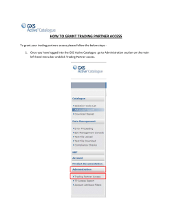

© Copyright 2026