
STABiX Documentation
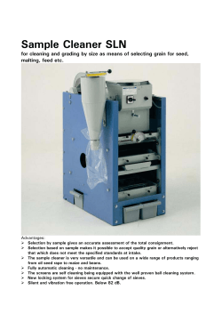
STABiX Documentation
Release 1.5.0
Mercier D., Zambaldi C. and Bieler T.R.
January 07, 2015
Contents
1
Contents
1.1 Motivation of this Work . . . . . . . . . . . . . . . . . . . . . . . . . . .
1.2 Getting started . . . . . . . . . . . . . . . . . . . . . . . . . . . . . . . .
1.3 Bicrystal Definition . . . . . . . . . . . . . . . . . . . . . . . . . . . . .
1.4 Strain Transfer Across Grain Boundaries . . . . . . . . . . . . . . . . . .
1.5 Experimental data . . . . . . . . . . . . . . . . . . . . . . . . . . . . . .
1.6 EBSD map GUI . . . . . . . . . . . . . . . . . . . . . . . . . . . . . . .
1.7 Bicrystal GUI . . . . . . . . . . . . . . . . . . . . . . . . . . . . . . . . .
1.8 CPFE simulation preprocessing GUIs . . . . . . . . . . . . . . . . . . . .
1.9 Analysis of literature data . . . . . . . . . . . . . . . . . . . . . . . . . .
1.10 A Matlab toolbox to analyze grain boundary inclination from SEM images
.
.
.
.
.
.
.
.
.
.
.
.
.
.
.
.
.
.
.
.
.
.
.
.
.
.
.
.
.
.
.
.
.
.
.
.
.
.
.
.
.
.
.
.
.
.
.
.
.
.
.
.
.
.
.
.
.
.
.
.
.
.
.
.
.
.
.
.
.
.
.
.
.
.
.
.
.
.
.
.
.
.
.
.
.
.
.
.
.
.
.
.
.
.
.
.
.
.
.
.
.
.
.
.
.
.
.
.
.
.
.
.
.
.
.
.
.
.
.
.
.
.
.
.
.
.
.
.
.
.
.
.
.
.
.
.
.
.
.
.
3
3
4
5
7
13
16
18
20
23
25
2
References
29
3
Contact
31
4
Contributors
33
5
Acknowledgements
35
6
Keywords
37
i
ii
STABiX Documentation, Release 1.5.0
Figure 1: Slip transmission analysis for an EBSD map of near alpha phase Ti alloy.
The Matlab toolbox STABiX provides a unique and simple way to analyse slip transmission in a bicrystal. Graphical
User Interfaces (GUIs) are implemented in order to import EBSD results, and to represent and quantify grain boundary
slip resistance. Key parameters, such as the number of phases, crystal structure (fcc, bcc, or hcp), and slip families for
calculations, are set by the user. With this information, grain boundaries are plotted and color coded according to the
𝑚′ factor 1 that quantifies the geometrical compatibility of the slip planes normals and Burgers vectors of incoming and
outgoing slip systems. Other potential functions that could assess the potential to develop damage are implemented
(e.g. residual Burgers vector 2 and 3 , 𝑁 factor 4 , resolved shear stress 5 , misorientation...).
Furthermore, the GUI provides the possibility to plot and analyze the case of a bicrystal, and to model sphero-conical
indentation performed close to grain boundaries (i.e. quasi bicrystal deformation). All of the data linked to the
bicrystal indentation (indenter properties, indentation settings, grain boundary inclination, etc.) are collected through
the GUI. A pythonTM file can be then exported in order to carry out a fully automatic 3D crystal plasticity finite
element simulations of the indentation process using one of the constitutive models available in DAMASK 6 and 7 .
The plasticity of single crystals is quantified by a combination of crystal lattice orientation mapping, instrumented
sphero-conical indentation, and measurement of the resulting surface topography 8 and 9 . In this way the stress and
strain fields close to the grain boundary can be rapidly assessed. Activation and transmission of slip are interpreted
based on these simulations and the mechanical resistance of grain boundaries can be quantified.
First of all, download the source code of the Matlab toolbox.
Source code is hosted at Github.
1 J. Luster and M.A. Morris, “Compatibility of deformation in two-phase Ti-Al alloys: Dependence on microstructure and orientation relationships.”, Metal. and Mat. Trans. A (1995), 26(7), pp. 1745-1756.
2 M.J. Marcinkowski and W.F. Tseng, “Dislocation behavior at tilt boundaries of infinite extent.”, Metal. Trans. (1970), 1(12), pp. 3397-3401.
3 W. Bollmann, “Crystal Defects and Crystalline Interfaces”, Springer-Verlag (1970).
4 J.D. Livingston and B. Chalmers, “Multiple slip in bicrystal deformation.”, Acta Metallurgica (1957), 5(6), pp. 322-327.
5 T.R. Bieler et al., “The role of heterogeneous deformation on damage nucleation at grain boundaries in single phase metals.”, Int. J. of Plast.
(2009), 25(9), pp. 1655–1683.
6 F. Roters et al., “Overview of constitutive laws, kinematics, homogenization and multiscale methods in crystal plasticity finite-element modeling: Theory, experiments, applications.”, Acta Materialia (2010), 58(4), pp. 1152-1211.
7 DAMASK — the Düsseldorf Advanced Material Simulation Kit.
8 C. Zambaldi et al., “Orientation informed nanoindentation of 𝛼-titanium: Indentation pileup in hexagonal metals deforming by prismatic slip”,
J. Mater. Res. (2012), 27(01), pp. 356-367.
9 C. Zambaldi, “Anisotropic indentation pile-up in single crystals”.
Contents
1
STABiX Documentation, Release 1.5.0
Download source code as a .zip file.
Find here the reference paper for this toolbox.
Download the documentation as a pdf file.
2
Contents
CHAPTER 1
Contents
1.1 Motivation of this Work
The micromechanical behavior of grain boundaries is one of the key components in the understanding of heterogeneous
deformation of metals 1 . To investigate the nature of the strengthening effect of grain boundaries, slip transmission
across interfaces has been investigated through bicrystal deformation experiments during the sixty past decades 2 , 3 ,
4 5 6 7 8 9 10 11 12 13 14
, , , , , , , , , , and 15 . Originally, interactions between dislocations and grain boundaries have been
observed in the transmission electron microscope (TEM) after strain test or in situ 4 , 5 and 15 . Some authors observed
as well slip transmission during indentation tests performed close to grain boundaries 16 , 17 , 18 , 19 and 20 .
To better understand the role played by the grain boundaries, we developed a Matlab Toolbox with Graphical User
Interfaces (GUI), to analyze and to quantify the micromechanics of grain boundaries. This toolbox aims to link
experimental results to crystal plasticity finite element (CPFE) simulations 21 .
1
T.R. Bieler et al., “Grain boundaries and interfaces in slip transfer.”, Current Opinion in Solid State and Materials Science (2014), in press.
K.T. Aust et al., “Solute induced hardening near grain boundaries in zone refined metals.”, Acta Metallurgica (1968), 16(3), pp. 291-302.
3 J.D. Livingston and B. Chalmers, “Multiple slip in bicrystal deformation.”, Acta Metallurgica (1957), 5(6), pp. 322-327.
4 Z. Shen et al., “Dislocation pile-up and grain boundary interactions in 304 stainless steel.”, Scripta Metallurgica (1986), 20(6), pp. 921–926.
5 Z. Shen et al., “Dislocation and grain boundary interactions in metals.”, Acta Metallurgica (1988), 36(12), pp. 3231–3242.
6 J. Luster and M.A. Morris, “Compatibility of deformation in two-phase Ti-Al alloys: Dependence on microstructure and orientation relationships.”, Metal. and Mat. Trans. A (1995), 26(7), pp. 1745-1756.
7 M.J. Marcinkowski and W.F. Tseng, “Dislocation behavior at tilt boundaries of infinite extent.”, Metal. Trans. (1970), 1(12), pp. 3397-3401.
8 W. Bollmann, “Crystal Defects and Crystalline Interfaces”, Springer-Verlag (1970)
9 L.C. Lim and R. Raj, “Continuity of slip screw and mixed crystal dislocations across bicrystals of nickel at 573K.”, Acta Metallurgica (1985),
33, pp. 1577.
10 T.C. Lee et al., “Prediction of slip transfer mechanisms across grain boundaries.”, Scripta Metallurgica, (1989), 23(5), pp. 799–803.
11 T.C. Lee et al., “An In Situ transmission electron microscope deformation study of the slip transfer mechanisms in metals”, Metallurgical
Transactions A (1990), 21(9), pp. 2437-2447.
12 W.A.T. Clark et al., “On the criteria for slip transmission across interfaces in polycrystals.”, Scripta Metallurgica et Materialia (1992), 26(2),
pp. 203–206.
13 W.Z. Abuzaid et al., “Slip transfer and plastic strain accumulation across grain boundaries in Hastelloy X.”, J. of the Mech. and Phys. of Sol.
(2012), 60(6) ,pp. 1201–1220.
14 J.R. Seal et al., “Analysis of slip transfer and deformation behavior across the 𝛼/𝛽 interface in Ti–5Al–2.5Sn (wt.%) with an equiaxed
microstructure.”, Mater. Sc. and Eng.: A (2012), 552, pp. 61-68.
15 J. Kacher et al., “Dislocation interactions with grain boundaries.”, Current Opinion in Solid State and Materials Science (2014), in press.
16 P.C. Wo and A.H.W. Ngan, “Investigation of slip transmission behavior across grain boundaries in polycrystalline Ni3Al using nanoindentation.”, J. Mater. Res. (2004), 19(1), pp. 189-201.
17 W.A. Soer et al. ,”Incipient plasticity during nanoindentation at grain boundaries in body-centered cubic metals.”, Acta Materialia (2005), 53,
pp. 4665–4676.
18 T.B. Britton et al., “Nanoindentation study of slip transfer phenomenon at grain boundaries.”, J. Mater. Res., 2009, 24(3), pp. 607-615.
19 S. Patthak et al., “Studying grain boundary regions in polycrystalline materials using spherical nano-indentation and orientation imaging
microscopy.”, J. Mater. Sci. (2012), 47, pp. 815–823.
20 S.K. Lawrence et al., “Grain Boundary Contributions to Hydrogen-Affected Plasticity in Ni-201.”, The Journal of The Minerals, Metals &
Materials Society (2014), 66(8), pp. 1383-1389.
21 DAMASK — the Düsseldorf Advanced Material Simulation Kit
2
3
STABiX Documentation, Release 1.5.0
1.1.1 Strategy
Comparison of topographies of indentations at grain boundaries to simulated indentations as predicted by 3D CPFE
modelling.
The goals of this research are:
1 - Carry out indentation within the interiors of large grains of alpha-titanium to effectively collect single crystal
data coupled with extensive (three-dimensional) characterization of the resulting plastic defect fields surrounding the
indents 22 . By correlating with models of the indentation, a precise constitutive description of the anisotropic plasticity
of single-crystalline titanium shall be developed 23 and 23 .
2 - Extension of this methodology to indentations close to grain boundaries, i.e. quasi bi-crystal deformation.
3 - Comparison of the measured characteristics of indentations at grain boundaries to simulated indentations as predicted by a constitutive model calibrated using the single crystal indentations.
4 - Based on this qualitative understanding, a grain boundary transmissivity description will be developed validated
against the collected indent characteristics.
1.2 Getting started
First of all, download the source code of the Matlab toolbox.
Source code is hosted at Github.
Download source code as a .zip file.
To have more details about the use of the toolbox, please have a look to :
README.txt
Then, run the following Matlab script and answer ‘y’ or ‘yes’ to add path to the Matlab search paths :
path_management.m
Run one of these GUIs to play with the toolbox.
Matlab
function
demo.m
EBSD map GUI
Bicrystal BUI
preCPFE_SX
preCPFE_BX
GBinc
Features
Start and run other GUIs.
Analysis of slip transmission across GBs for an EBSD
map.
Analysis of slip transfer in a bicrystal.
Preprocess of CPFE model for SX indentation.
Preprocess of CPFE model for BX indentation.
Calculation of grain boundaries inclination.
YAML config. file
config_gui_EBSDmap_default.yaml
config_CPFEM_default.yaml
config_CPFEM_default.yaml
Default YAML configuration files, stored in the folder YAML_config_files, are loaded automatically to set the GUIs:
22 C. Zambaldi et al., “Orientation informed nanoindentation of 𝛼-titanium: Indentation pileup in hexagonal metals deforming by prismatic slip”,
J. Mater. Res. (2012), 27(01), pp. 356-367.
23 F. Roters et al., “Overview of constitutive laws, kinematics, homogenization and multiscale methods in crystal plasticity finite-element modeling: Theory, experiments, applications.”, Acta Materialia (2010), 58(4), pp. 1152-1211.
4
Chapter 1. Contents
STABiX Documentation, Release 1.5.0
config.yaml
config_CPFEM_defaults.yaml
config_CPFEM_material_defaults.yaml
config_CPFEM_materialA_defaults.yaml
config_CPFEM_materialB_defaults.yaml
config_gui_EBSDmap_defaults.yaml
config_gui_BX_defaults.yaml
config_gui_SX_defaults.yaml
config_mesh_BX_defaults.yaml
config_mesh_SX_defaults.yaml
You have to set your own YAML configuration files, by following instructions given in this README.
If the OpenGL rendering is not satisfying, you can modify the corresponding option in the config.yaml file.
Visit the YAML website for more informations.
Visit the YAML code for Matlab.
Visit the Matlab page about OpenGL rendering.
1.3 Bicrystal Definition
1.3.1 Crystallographic properties of a bicrystal
A bicrystal is formed by two adjacent crystals separated by a grain boundary.
Five macroscopic degrees of freedom are required to characterize a grain boundary 24 , 25 , 26 and 27 :
• 3 for the rotation between the two crystals;
• 2 for the orientation of the grain boundary plane defined by its normal 𝑛.
The rotation between the two crystals is defined by the rotation angle 𝜔 and the rotation axis common to both crystals
[𝑢𝑣𝑤].
Using orientation matrix of both crystals obtained by EBSD measurements, the misorientation or disorientation matrix
(∆𝑔) or (∆𝑔d ) is calculated 28 and 29 :
∆𝑔 = 𝑔B 𝑔A−1 = 𝑔A 𝑔B−1
(1.1)
∆𝑔d = (𝑔B * 𝐶𝑆)(𝐶𝑆 −1 * 𝑔A−1 ) = (𝑔A * 𝐶𝑆)(𝐶𝑆 −1 * 𝑔B−1 )
(1.2)
Disorientation describes the misorientation with the smallest possible rotation angle and 𝐶𝑆 denotes one of the symmetry operators for the material 30 .
The Matlab function used to set the symmetry operators is: sym_operators.m
The orientation matrix 𝑔 of a crystal is calculated from the Euler angles (𝜑1 , Φ, 𝜑2 ) using the following equation :
28
V. Randle and O. Engler, “Introduction to Texture Analysis: Macrotexture, Microtexture and Orientation Mapping.”, CRC Press (2000).
A. Morawiec, “Orientations and Rotations: Computations in Crystallographic Textures.”, Springer, 2004.
30 U.F. Kocks et al., “Texture and Anisotropy: Preferred Orientations in Polycrystals and Their Effect on Materials Properties.” Cambridge
University Press (2000).
29
1.3. Bicrystal Definition
5
STABiX Documentation, Release 1.5.0
⎛
cos(𝜑1 ) cos(𝜑2 ) − sin(𝜑1 ) sin(𝜑2 ) cos(Φ)
sin(𝜑1 ) cos(𝜑2 ) + cos(𝜑1 ) sin(𝜑2 ) cos(Φ)
𝑔 = ⎝− cos(𝜑1 ) sin(𝜑2 ) − sin(𝜑1 ) cos(𝜑2 ) cos(Φ) − sin(𝜑1 ) sin(𝜑2 ) + cos(𝜑1 ) cos(𝜑2 ) cos(Φ)
sin(𝜑1 ) sin(Φ)
− cos(𝜑1 ) sin(Φ)
⎞
sin(𝜑2 ) sin(Φ)
cos(𝜑2 ) sin(Φ)⎠
cos(Φ)
(1.3)
The orientation of a crystal (Euler angles) can be determined via electron backscatter diffraction (EBSD) measurement
or via transmission electron microscopy (TEM).
The Matlab function used to generate random Euler angles is: randBunges.m
The Matlab function used to calculate the orientation matrix from Euler angles is: eulers2g.m
The Matlab function used to calculate Euler angles from the orientation matrix is: g2eulers.m
Then, from this misorientation matrix (∆𝑔), the rotation angle (𝜔) and the rotation axis [𝑢, 𝑣, 𝑤] can be obtained by
the following equations :
𝜔 = cos−1 ((𝑡𝑟(∆𝑔) − 1)/2)
(1.4)
𝑢 = ∆𝑔23 − ∆𝑔32
𝑣 = ∆𝑔31 − ∆𝑔13
(1.5)
𝑤 = ∆𝑔12 − ∆𝑔21
The Matlab function used to calculate the misorientation angle is: misorientation.m
The grain boundary plane normal 𝑛 can be determined knowing the grain boundary trace angle 𝛼 and the grain
boundary inclination 𝛽.
The grain boundary trace angle is obtained through the EBSD measurements (grain boundary endpoints coordinates)
and the grain boundary inclination can be assessed by a serial polishing (chemical-mechanical polishing or FIB sectioning), either parallel or perpendicular to the surface of the sample (see Figure 2).
Figure 1.1: Figure 1 : Schematic of a bicrystal.
6
Chapter 1. Contents
STABiX Documentation, Release 1.5.0
Figure 1.2: Figure 2 : Screenshot of the Matlab GUI used to calculate grain boundary inclination.
1.4 Strain Transfer Across Grain Boundaries
The strain transfer across grain boundaries can be defined by the four following mechanisms (see Figure 1) 31 , 32 , 33
and 34 :
1. direct transmission with slip systems having the same Burgers vector, and the grain boundary is transparent to
dislocations (no strengthening effect) (Figure 1-a);
2. direct transmission, but slip systems have different Burgers vector (leaving a residual boundary dislocations)
(Figure 1-b);
3. indirect transmission, and slip systems have different Burgers vector (leaving a residual boundary dislocations)
(Figure 1-c);
4. no transmission and the grain boundary acts as an impenetrable boundary, which implies stress accumulations,
localized rotations, pile-up of dislocations... (Figure 1-d).
Figure 1.3: Figure 1 : Possible strain transfer across grain boundaries (GB) from Sutton and Balluffi.
Several authors proposed slip transfer parameters from modellings or experiments for the last 60 years. A nonexhaustive list of those criteria is given in the next part of this work, including geometrical parameter, stress and
31 L.C. Lim and R. Raj, “Continuity of slip screw and mixed crystal dislocations across bicrystals of nickel at 573K.”, Acta Metallurgica (1985),
33, pp. 1577.
32 A.P. Sutton and R.W. Balluffi, “Interfaces in Crystalline Materials.”, OUP Oxford (1995).
33 S. Zaefferer et al., “On the influence of the grain boundary misorientation on the plastic deformation of aluminum bicrystals.”, Acta Materialia
(2003), 51(16), pp. 4719-4735.
34 L. Priester, “Grain Boundaries: From Theory to Engineering.”, Springer Series in Materials Science (2013).
1.4. Strain Transfer Across Grain Boundaries
7
STABiX Documentation, Release 1.5.0
energetic functions, and recent combinations of the previous parameters.
1.4.1 Geometrical Criteria
Based on numerous investigations of dislocation-grain boundary interactions, quantitative geometrical expressions
describing the slip transmission mechanisms have been developed. A non-exhaustive list of geometrical criteria is
detailed subsequently. The geometry of the slip transfer event is most of the time described by the scheme given
Figure 2. 𝜅 is the angle between slip directions, 𝜃 is the angle between the two slip plane intersections with the
grain boundary, 𝜓 is the angle between slip plane normal directions, 𝛾 is the angle between the direction of incoming
slip and the plane normal of outgoing slip, and 𝛿 is between the direction of outgoing slip and the plane normal of
incoming slip. 𝑛, 𝑑 and 𝑙 are respectively the slip plane normals, slip directions and the lines of intersection of the
slip plane and the grain boundary. ⃗𝑏 is the Burgers vector of the slip plane and ⃗𝑏r is the residual Burgers vector of the
residual dislocation at the grain boundary. The subscripts in and out refer to the incoming and outgoing slip systems,
respectively.
Figure 1.4: Figure 2 : Geometrical description of the slip transfer.
• 𝑁 factor from Livingston and Chalmers in 1957 35
𝑁 = (⃗𝑛in · ⃗𝑛out )(𝑑⃗in · 𝑑⃗out ) + (⃗𝑛in · 𝑑⃗out )(⃗𝑛out · 𝑑⃗in )
(1.6)
𝑁 = cos 𝜓 cos 𝜅 + cos 𝛾 cos 𝛿
(1.7)
Many authors referred to this criterion to analyze slip transmission 36 , 37 , 38 , 39 , 40 , 41 , 42 , 43 , 44 and 45 . Pond et
al. proposed to compute this geometric criteria for hexagonal metals using Frank’s method 46 .
35
J.D. Livingston and B. Chalmers, “Multiple slip in bicrystal deformation.”, Acta Metallurgica (1957), 5(6), pp. 322-327.
J.J. Hauser and B. Chamlers, “The plastic deformation of bicrystals of f.c.c. metals.”, Acta Metallurgica (1961), 9(9), pp. 802-818.
37 K.G. Davis et al., “Slip band continuity across grain boundaries in aluminum.”, Acta Metallurgica (1966), 14, pp. 1677-1684.
38 R.E. Hook and J.P. Hirth, “The deformation behavior of isoaxial bicrystals of Fe-3%Si.”, Acta Metallurgica (1967), 15(3), pp. 535-551.
39 R.E. Hook and J.P. Hirth, “The deformation behavior of non-isoaxial bicrystals of Fe-3% Si.”, Acta Metallurgica(1967), 15(7), pp. 1099-1110.
40 Z. Shen et al., “Dislocation pile-up and grain boundary interactions in 304 stainless steel.”, Scripta Metallurgica (1986), 20(6), pp. 921–926.
41 Z. Shen et al., “Dislocation and grain boundary interactions in metals.”, Acta Metallurgica (1988), 36(12), pp. 3231–3242.
42 T.C. Lee et al., “TEM in situ deformation study of the interaction of lattice dislocations with grain boundaries in metals.”, Philosophical
Magazine A (1990), 62(1), pp. 131-153.
43 T.C. Lee et al., “An In Situ transmission electron microscope deformation study of the slip transfer mechanisms in metals”, Metallurgical
Transactions A (1990), 21(9), pp. 2437-2447.
44 W.A.T. Clark et al., “On the criteria for slip transmission across interfaces in polycrystals.”, Scripta Metallurgica et Materialia (1992), 26(2),
pp. 203–206.
45 M. Ueda et al., “Effect of grain boundary on martensite transformation behaviour in Fe–32 at.%Ni bicrystals.”, Science and Technology of
Advanced Materials (2002), 3(2), pp. 171.
46 R.C. Pond et al., “On the crystallography of slip transmission in hexagonal metals.”, Scripta Metallurgica (1986), 20, pp. 1291-1295.
36
8
Chapter 1. Contents
STABiX Documentation, Release 1.5.0
The Matlab function used to calculate the N factor is: N_factor.m
• 𝐿𝑅𝐵 factor from Shen et al. in 1986 66 and 67
𝐿𝑅𝐵 = (⃗𝑙in · ⃗𝑙out )(𝑑⃗in · 𝑑⃗out )
(1.8)
𝐿𝑅𝐵 = cos 𝜃 cos 𝜅
(1.9)
The original notation of this 𝐿𝑅𝐵 factor is 𝑀 , but unfortunately this notation is often used for the Taylor factor
. Pond et al. proposed to compute this geometric criteria for hexagonal metals using Frank’s method 58 .
Recently, Spearot and Sangid have plotted this parameter as a function of the misorientation of the bicrystal
using atomistic simulations 48 .
47
49 43 44 14 50 51 52 53 54
, , , , , , , , and 55 mentioned in their respective studies this geometrical parameter as a condition
for slip transmission.
The inclination of the grain boundary (𝛽) is required to evaluate this factor and the 𝐿𝑅𝐵 or 𝑀 factor should be
maximized.
The Matlab function used to calculate the LRB factor is: LRB_parameter.m
• 𝑚′ parameter from Luster and Morris in 1995 56
𝑚′ = (⃗𝑛in · ⃗𝑛out )(𝑑⃗in · 𝑑⃗out )
(1.10)
𝑚′ = cos 𝜓 cos 𝜅
(1.11)
Many authors found that this 𝑚′ parameter, which takes into account the degree of coplanarity of slip systems,
is promising to predict slip transmission 57 , 58 , 59 , 60 , 8 and 61 . Both 𝑚′ and 𝐿𝑅𝐵 can be easily assessed in
computational experiments 8 . This 𝑚′ factor should be maximized (1 means grain boundary is transparent and
0 means grain boundary is an impenetrable boundary).
47 T.R. Bieler et al., “Grain boundaries and interfaces in slip transfer.”, Current Opinion in Solid State and Materials Science, (2014), 18(4), pp.
212-226.
48 D.E. Spearot and M.D. Sangid, “Insights on slip transmission at grain boundaries from atomistic simulations.”, Current Opinion in Solid State
and Materials Science (2014), in press.
49 T.C. Lee et al., “Prediction of slip transfer mechanisms across grain boundaries.”, Scripta Metallurgica, (1989), 23(5), pp. 799–803.
50 T. Kehagias et al., “Slip transfer across low-angle grain boundaries of deformed titanium.”, Interface Science (1995), 3(3), pp. 195-201.
51 T. Kehagias et al., “Pyramidal Slip in Electron Beam Heated Deformed Titanium.”, Scripta Metallurgica et Materialia (1996), 33(12), pp.
1883-1888.
52 W.M. Ashmawi and M.A. Zikry, “Prediction of Grain-Boundary Interfacial Mechanisms in Polycrystalline Materials.”, Journal of Engineering
Materials and Technology (2001), 124(1), pp. 88-96.
53 A. Gemperle et al., “Interaction of slip dislocations with grain boundaries in body-centered cubic bicrystals.”, Materials Science and Engineering A (2004), 378-389, pp. 46-50.
54 J. Gemperlova et al.,”Slip transfer across grain boundaries in Fe–Si bicrystals.”, Journal of Alloys and Compounds (2004), 378(1-2), pp.
97-101.
55 J. Shi and M.A. Zikry, “Modeling of grain boundary transmission, emission, absorption and overall crystalline behavior in Σ1, Σ3, and Σ17b
bicrystals.”, J. Mater. Res., (2011), 26(14), pp. 1676-1687.
56 J. Luster and M.A. Morris, “Compatibility of deformation in two-phase Ti-Al alloys: Dependence on microstructure and orientation relationships.”, Metal. and Mat. Trans. A (1995), 26(7), pp. 1745-1756.
57 M.G. Wang and A.H.W. Ngan,”Indentation strain burst phenomenon induced by grain boundaries in niobium.”, Journal of Materials Research
(2004), 19(08), pp. 2478-2486.
58 P.C. Wo and A.H.W. Ngan, “Investigation of slip transmission behavior across grain boundaries in polycrystalline Ni3Al using nanoindentation.”, J. Mater. Res. (2004), 19(1), pp. 189-201.
59 T.B. Britton et al., “Nanoindentation study of slip transfer phenomenon at grain boundaries.”, J. Mater. Res., (2009), 24(3), pp. 607-615.
60 T.R. Bieler et al., “The role of heterogeneous deformation on damage nucleation at grain boundaries in single phase metals.”, Int. J. of Plast.
(2009), 25(9), pp. 1655–1683.
61 Y. Guo et al., “Slip band–grain boundary interactions in commercial-purity titanium.”, Acta Materialia (2014), 76, pp. 1-12.
1.4. Strain Transfer Across Grain Boundaries
9
STABiX Documentation, Release 1.5.0
Figure 1.5: Figure 3 : Distribution of m’ parameter in function of angles values.
Figure 1.6: Figure 4 : Distribution of m’ parameter calculated for prismatic <a> slip systems in function of misorientation angle.
A resistance factor of the grain boundary can be described by the following equation :
𝐺𝐵resfac = 1 − 𝑚′
10
(1.12)
Chapter 1. Contents
STABiX Documentation, Release 1.5.0
This factor is equal to 0 (grain boundary transparent if the 𝑚′ parameter is equal to 1 (when slip perfectly
aligns)).
The Matlab function used to calculate the m’ parameter is: mprime.m
• ⃗𝑏r the residual Burgers vector 62 , 63 , 46 , 64 , 65 , 44 and 14 .
⃗𝑏r = ⃗𝑔in · ⃗𝑏in − ⃗𝑔out · ⃗𝑏out
(1.13)
The magnitude of this residual Burgers vector should be minimized.
Shirokoff et al., Kehagias et al., and Kacher et al. used the residual Burgers vector as a criterion to analyse slip
transmission in cp-Ti (hex) 66 , 37 , 38 and 67 , Lagow et al. in Mo (bcc) 68 , Gemperle et al. and Gemperlova et al.
in FeSi (bcc) 25 and 26 , Kacher et al. in 304 stainless steel (fcc) 69 , and Jacques et al. for semiconductors 70 .
Patriarca et al. demonstrated for BCC material the role of the residual Burgers vector in predicting slip transmission, by analysing strain field across GBs determined by digital image correlation 71 .
Misra and Gibala used the residual Burgers vector to analyze slip across a fcc/bcc interphase boundary 72 .
The Matlab function used to calculate the residual Burgers vector is: residual_Burgers_vector.m
• The misorientation or disorientation (∆𝑔 or ∆𝑔d ) 73 , 74 and 80
It has been observed during first experiments of bicrystals deformation in 1954, that the yield stress and the rate
of work hardening increased with the orientation difference between the crystals 3 and 12 .
Some authors demonstrated a strong correlation between misorientation between grains in a bicrystal and the
grain boundary energy through crystal plasticity finite elements modelling and molecular dynamics simulations
74 75 76 77 78
, , , , and 79 . Some authors studied the stability of grain boundaries by the calculations of energy
difference vs. misorientation angle through the hexagonal c-axis/a-axis 80 .
The misorientation and disorientation equations are given in the crystallographic properties of a bicrystal.
The Matlab function used to calculate the misorientation angle is: misorientation.m
66
J. Shirokoff et al., “The Slip Transfer Process Through Grain Boundaries in HCP Ti.”, MRS Online Proceedings Library (1993), 319, pp.
263-272.
67 J. Kacher and I.M. Robertson, “In situ and tomographic analysis of dislocation/grain boundary interactions in 𝛼-titanium.”, Philosophical
Magazine (2014), 94(8), pp. 814-829.
68 B.W. Lagow, “Observation of dislocation dynamics in the electron microscope.”, Materials Science and Engineering: A, 2001, 309–310, pp.
445-450.
69 J. Kacher and I.M. Robertson, “Quasi-four-dimensional analysis of dislocation interactions with grain boundaries in 304 stainless steel.”, Acta
Materialia (2012), 60(19), pp. 6657–6672.
70 A. Jacques et al., “New results on dislocation transmission by grain boundaries in elemental semiconductors.”, Le Journal de Physique
Colloques (1990), 51(C1), pp. 531-536.
71 L. Patriarca et al., “Slip transmission in bcc FeCr polycrystal.”, Materials Science&Engineering (2013), A588, pp. 308–317.
72 A. Misra and R. Gibala, “Slip Transfer and Dislocation Nucleation Processes in Multiphase Ordered Ni-Fe-Al Alloys”, Metallurgical and
Materials Trans. A (1999), 30A, pp. 991-1001.
73 K.T. Aust and N.K. Chen, “Effect of orientation difference on the plastic deformation of aluminum bicrystals.”, Acta Metallurgica (1954), 2,
pp. 632-638.
74 W.A.T. Clark and B. Chalmers, “Mechanical deformation of aluminium bicrystals.”, Acta Metallurgica (1954), 2(1), pp. 80-86.
75 A. Ma et al., “On the consideration of interactions between dislocations and grain boundaries in crystal plasticity finite element modeling –
Theory, experiments, and simulations.”, Acta Materialia (2006), 54(8), pp.2181-2194.
76 Z. Li et al., “Strengthening mechanism in micro-polycrystals with penetrable grain boundaries by discrete dislocation dynamics simulation
and Hall–Petch effect.”, Computational Materials Science (2009), 46(4), pp. 1124-1134.
77 D.V. Bachurin et al., “Dislocation–grain boundary interaction in <111> textured thin metal films.”, Acta Materialia (2010), 58, pp. 5232–5241.
78 M.D. Sangid et al., “Energy of slip transmission and nucleation at grain boundaries.”, Acta Materialia (2011), 59(1), pp. 283–296.
79 M.D. Sangid et al., “Energetics of residual dislocations associated with slip–twin and slip–GBs interactions.”, Materials Science and Engineering A (2012), 542, pp. 21–30.
80 H. Faraoun et al., “Study of stability of twist grain boundaries in hcp zinc.”, Scripta Materialia (2006), 54, pp. 865–868.
1.4. Strain Transfer Across Grain Boundaries
11
STABiX Documentation, Release 1.5.0
1.4.2 Stress Criteria
• Schmid Factor (𝑚) 81 , 82 and 83
The Schmid’s law can be expressed by the following equation:
𝜏 𝑖 = 𝜎 : 𝑆0 𝑖
(1.14)
𝑆0 𝑖 = 𝑑⃗𝑖 ⊗ ⃗𝑛𝑖
(1.15)
𝜎 is an arbitrary stress state and 𝜏 𝑖 the resolved shear stress on slip system 𝑖. 𝑆0 𝑖 is the Schmid matrix defined
by the dyadic product of the slip plane normals ⃗𝑛 and the slip directions 𝑑⃗ of the slip system 𝑖. The Schmid
factor, 𝑚, is defined as the ratio of the resolved shear stress 𝜏 𝑖 to a given uniaxial stress.
Knowing the value of the highest Schmid factor of a given slip system for both grains in a bicrystal, Abuzaid et
al. 1 proposed the following criterion :
𝑚GB = 𝑚in + 𝑚out
(1.16)
The subscripts GB, in, and out refer to the grain boundary, and the incoming and outgoing slip systems, respectively. This GB Schmid factor (𝑚GB ) factor should be maximized.
The Matlab function used to calculate the Schmid factor is: resolved_shear_stress.m
• Generalized Schmid Factor (𝐺𝑆𝐹 ) 61 and 8
The generalized Schmid factor, which describes the shear stress on a given slip system, can be computed from
any stress tensor 𝜎 based on the Frobenius norm of the tensor.
𝐺𝑆𝐹 = 𝑑⃗ · 𝑔𝜎𝑔 · ⃗𝑛
(1.17)
⃗𝑛 and 𝑑⃗ are respectively the slip plane normals and the slip directions of the slip system. The 𝑔 is the orientation
matrix for a given crystal.
The Matlab function used to calculate the generalized Schmid factor is: generalized_schmid_factor.m
• Resolved Shear Stress (𝜏 ) 42 , 43 , 44 , 14 , 40 , 7 , 84 , 85 and 86
The resolved shear stress 𝜏 acting on the outgoing slip system from the piled-up dislocations should be maximized. This criterion considers the local stress state.
The resolved shear stress on the grain boundary should be minimized.
81
C.N. Reid, “Deformation Geometry for Materials Scientists.”, Pergamon Press, Oxford, United Kingdom, 1973.
J.R. Seal et al., “Analysis of slip transfer and deformation behavior across the 𝛼/𝛽 interface in Ti–5Al–2.5Sn (wt.%) with an equiaxed
microstructure.”, Mater. Sc. and Eng.: A (2012), 552, pp. 61-68.
83 W.Z. Abuzaid et al., “Slip transfer and plastic strain accumulation across grain boundaries in Hastelloy X.”, J. of the Mech. and Phys. of Sol.
(2012), 60(6) ,pp. 1201–1220.
84 M.P. Dewald et al., “Multiscale modelling of dislocation/grain-boundary interactions: I. Edge dislocations impinging on Σ11 (1 1 3) tilt
boundary in Al.”, Modelling Simul. Mater. Sci. Eng. (2007), 15(1).
85 M.P. Dewald et al., “Multiscale modelling of dislocation/grain boundary interactions. II. Screw dislocations impinging on tilt boundaries in
Al.”, Phil. Mag. (2007), 87(30), pp. 1655–1683.
86 M.P. Dewald et al., “Multiscale modeling of dislocation/grain-boundary interactions: III. 60° dislocations impinging on Σ3, Σ9 and Σ11 tilt
boundaries in Al.”, Modelling Simul. Mater. Sci. Eng. (2011), 19(5).
82
12
Chapter 1. Contents
STABiX Documentation, Release 1.5.0
For Shi and Zikry, the ratio of the resolved shear stress to the reference shear stress of the outgoing slip system
(stress ratio) should be greater than a critical value (which is approximately 1) 68 .
For Li et al. and Gao et al. the resolved shear stress acting on the incoming dislocation on the slip plane must
be larger than the critical penetration stress. From the energy point of view, only when the work by the external
force on the incoming dislocation is greater than the summation of the GB energy and strain energy of GB
dislocation debris, it is possible that the incoming dislocation can penetrate through the GB 45 and 87 .
It is possible to assess the shear stress from the geometrical factor 𝑁 (Livingston and Chamlers) :
𝜏in = 𝜏out * 𝑁
(1.18)
Where 𝜏out is the shear stress at the head of the accumulated dislocations in their slip plane and 𝜏in is the shear
acting on the incoming slip system 48 , 30 and 31 .
The Matlab function used to calculate the resolved shear stress is: resolved_shear_stress.m
1.4.3 Combination of Criteria
• Geometrical function weighted by the accumulated shear stress or the Schmid factor
mented...)
8
(not yet imple-
1.4.4 Slip transmission parameters implemented in the Matlab Toolbox
Slip transmission parameter
Function
Matlab function
Reference
Misorientation angle (𝜔)
C-axis misorientation angle (hcp
material) (𝜔)
𝑁 factor from Livingston and
Chamlers
𝐿𝑅𝐵 factor from Shen et al.
𝑚′ parameter from Luster and Morris
residual Burgers vector (⃗𝑏r )
𝜔 = 𝑐𝑜𝑠−1 ((𝑡𝑟(∆𝑔) − 1)/2)
misorientation.m
c-axis misorientation.m
74
N_factor.m
48
LRB_parameter.m
mprime.m
residual_Burgers_vector.m
resolved_shear_stress.m
66
resolved_shear_stress.m
generalized_schmid_factor.m
1
Resolved Shear Stress (𝜏 𝑖 ) / Schmid
Factor
Grain boundary Schmid factor
Generalized Schmid Factor (𝐺𝑆𝐹 )
𝑁=
cos(𝜓) · cos(𝜅) + cos(𝛾) · cos(𝛿)
𝐿𝑅𝐵 = cos(𝜃) · cos(𝜅)
𝑚′ = cos(𝜓) · cos(𝜅)
⃗𝑏r = 𝑔in · ⃗𝑏in − 𝑔out · ⃗𝑏out
𝜏 𝑖 = 𝜎 : 𝑆0 𝑖 with 𝑆0 𝑖 = 𝑑 ⊗ 𝑛
𝑚GB = 𝑚in + 𝑚out
𝐺𝑆𝐹 = 𝑑 · 𝑔𝜎𝑔 · 𝑛
74
/ 67
49
51
61
61
1.4.5 References
1.5 Experimental data
To use the stabix toolbox, some experimental data are required :
87 Y. Gao et al., “A hierarchical dislocation-grain boundary interaction model based on 3D discrete dislocation dynamics and molecular dynamics.” Science China Physics, Mechanics and Astronomy (2011), 54(4), pp. 625-632.
1.5. Experimental data
13
STABiX Documentation, Release 1.5.0
• average grain orientations (Euler angles (𝜑1 , Φ, 𝜑2 ) in degrees) or intragranular misorientation (misorientation
axis [𝑢𝑣𝑤] / angle 𝜔);
• grains boundaries positions (optional for the bicrystal analysis);
• grains positions (optional for the bicrystal analysis);
• geometry of grain boundaries (trace angle and grain boundary inclination) (optional).
TEM experiments can provide intragranular misorientation and EBSD measurements can provide average grain orientations, grains boundaries and grains positions, and grain boundary trace angle.
Inclination of the grain boundary can be evaluated by serial polishing or focused ion beam (FIB) sectioning, either
parallel or perpendicular to the surface of the sample.
1.5.1 EBSD map GUI - TSL-OIM data preparation
Open you .osc (or your .ctf) file in the TSL-OIM Analysis Software.
Set the TSL coordinates system !
Change data properties for the detection of grain boundaries (All data –> Properties).
Clean up your dataset (Filename –> Cleanup).
Reference : OIM ANALYSIS 6.0 (user manual) / EDAX website
Reconstructed Boundaries File
Export “Reconstructed Boundaries File” of the cleaned dataset (All data –> Export –> Reconstructed Boundaries),
with the following options defined by default :
• Right hand average orientation (𝜑1 , Φ, 𝜑2 ) in degrees
• Left hand average orientation (𝜑1 , Φ, 𝜑2 ) in degrees
• Trace angle (in degrees)
• (𝑥, 𝑦) coordinates of endpoints (in microns)
• IDs of right hand and left hand grains
N.B : Reconstructed boundary methodology is only applied to data collected on a hexagonal grid. It is possible to
convert a square grid into an hexagonal grid in TSL-OIM software.
Example of “Reconstructed Boundary File”: MPIE_cpTi_reconstructed_boundaries_2013.txt
The Matlab function used to read “Reconstructed Boundary File” is: read_oim_reconstructed_boundaries_file.m
If some GBs segments are missing or some wrong segments are exported, play with partition properties in the TSL-OIM softwar
• decrease/increase “Grain Tolerance Angle”
• decrease/increase “Minimum Grain Size”
• decrease/increase the maximum deviation between reconstructed boundary and corresponding boundary
segments.
14
Chapter 1. Contents
STABiX Documentation, Release 1.5.0
Grain File Type 2
Export “Grain File Type 2” of the cleaned dataset (All data –> Export –> Grain File), with the following options :
• Integer identifying grain
• Average orientation (𝜑1 , Φ, 𝜑2 ) in degrees
• Average position (𝑥, 𝑦) in microns
• An integer identifying the phase
• Edge or interior grain (optional)
• Diameter of the grain in microns (optional)
N.B. : Export the “Grain File Type 2” in the same location as the corresponding “Reconstructed Boundary File”.
Example of “Grain Gile Type 2”: MPIE_cpTi_grain_file_type2_2013.txt
The Matlab function used to read “Grain File Type 2” is: read_oim_grain_file_type2.m
Scan Data (.ang file)
Export “Scan Data (.ang file)” of the cleaned dataset (Filename –> Export –> Scan Data) (optional).
This .ang file is useful for the MTEX Toolbox
Example of an .ang file.
Possible errors introduced during files exportation from TSL
• “Grain File Type 2” –> Missing integer identifying grain
– Solved when file is imported via the GUI.
• “Reconstructed Boundary File” –> Inversion of left and right grains for a given grain boundary
– Cross product performed between GB vector and center of grains to check (if cross product < 0 : no
inversion, and if cross product > 0 : inversion).
• “Reconstructed Boundary File” –> x-axis and y-axis not corrects. . .
– y coordinates is multiplied by -1 when file is imported via the GUI.
All of these issues are taken into account and corrected automatically when user is loading his data via the EBSD map
GUI.
1.5.2 Bicrystal GUI - YAML configuration file
The YAML configuration file provides a simple way to define a bicrystal.
An example of bicrystal configuration file is given here : config_gui_BX_defaults.yaml
Copy this example file and modify it with your data. Be careful to put a space after the comma in a list (e.g. [x, y, z]).
Don’t change fieldnames and don’t round Euler angles. Euler angles are given in degrees.
Load your YAML bicrystal configuration file via the menu in the bicrystal GUI.
Visit the YAML website for more informations.
Visit the YAML code for Matlab.
1.5. Experimental data
15
STABiX Documentation, Release 1.5.0
1.5.3 Convention for bicrystal EBSD/indentation experiments
Figure 1.7: Figure 1 : Geometrical convention of a bicrystal.
1.6 EBSD map GUI
This GUI allows to analyze quantitatively slip transmission across grain boundaries for an EBSD map.
The Matlab function used to run the EBSD map GUI is: A_gui_plotmap.m
This includes:
• Loading and Smoothing GBs segments
• Misorientation angle
• m’ parameter
• Residual Burgers vector
• Schmid factor and slip trace analysis
1.6.1 Loading and Smoothing GBs segments
Figure 1.8: Figure 1 : Screenshot of the EBSD map GUI with an EBSD map of a Ti alloy a) before smoothing and b)
after smoothing
16
Chapter 1. Contents
STABiX Documentation, Release 1.5.0
Figure 1.9: Figure 2 : Screenshot of the EBSD map GUI with an EBSD map of a Ti alloy (GBs color-coded in function
of the maximum misorientation angle value)
Figure 1.10: Figure 3 : Screenshot of the EBSD map GUI with an EBSD map of a Ti alloy (GBs color-coded in function
of the maximum m’ value)
Figure 1.11: Figure 4 : Screenshot of the EBSD map GUI with an EBSD map of a Ti alloy (GBs color-coded in function
of the maximum m’ value obtained for slips with the highest generalized Schmid factor)
1.6. EBSD map GUI
17
STABiX Documentation, Release 1.5.0
1.6.2 Misorientation angle
1.6.3 m’ parameter
1.6.4 Residual Burgers vector
Figure 1.12: Figure 5 : Screenshot of the EBSD map GUI with an EBSD map of a Ti alloy (GBs color-coded in function
of the maximum residual Burgers vector value)
1.6.5 Schmid factor and slip trace analysis
Figure 1.13: Figure 6 : Screenshot of the EBSD map GUI with an EBSD map of a Ti alloy (slip plane plotted inside
grain and slip traces plotted around unit cells, both in function of the maximum Schmid factor calculated with a given
stress tensor)
1.7 Bicrystal GUI
This GUI allows to analyze quantitatively slip transmission across grain boundaries for a single bicrystal selected from
the EBSD map plotted previously in the map GUI or set by the user (directly inside the bicrystal GUI or by loading a
YAML config. bicrystal file from the menu).
The Matlab function used to run the bicrystal GUI is: A_gui_plotGB_Bicrystal.m
This includes:
18
Chapter 1. Contents
STABiX Documentation, Release 1.5.0
• Plotting and analyzing a bicrystal
• Distribution of all slip transmission parameters
1.7.1 Plotting and analyzing a bicrystal
Figure 1.14: Figure 1 : Screenshot of the Bicrystal GUI
1.7.2 Distribution of all slip transmission parameters
It is possible to generate a new window, in which all values of the selected slip transmission parameter are plotted in
function of selected slip families.
Figure 1.15: Figure 2 : Screenshot of the distribution of all slip transmission parameters (e.g.: m’ parameter for a 1
phase (hcp) bicrystal)
1.7. Bicrystal GUI
19
STABiX Documentation, Release 1.5.0
1.8 CPFE simulation preprocessing GUIs
The preCPFE GUIs can rapidly transfer the experimental data into crystal plasticity finite element (CPFE) simulation
input files. The types of input files are :
• scripts to generate the finite element models in MSC.Mentat (procedure file format) or Abaqus (Python script)
based on the experimental data and test geometry ;
• the crystallographic orientations from the experimental data sets ;
• material parameter files for the subroutines that implement the constitutive model.
A parametrized visualization of the bicrystal indentation model through the GUI allows tuning the geometry and finite
element discretization and the size of the sample and the indenter.
Currently the following models can be written:
• Single crystal (SX) indentation (Mentat and Abaqus)
• Bicrystal (BX) indentation (Mentat and Abaqus)
1.8.1 Single crystal (SX) indentation
Analysis of the orientation dependent pile-up topographies that are formed during single crystal indentation provides
insight into the operating deformation mechanisms. CPFE simulation of single crystal indentation has an important
role in clarifying the influence of the single-slip behavior of different slip systems on the resulting surface profiles.
The function used to run the preCPFE GUI for SX indentation is: A_preCPFE_windows_indentation_setting_SX.m
Figure 1.16: Figure 1 : Screenshot of the preCPFE GUI for the single crystal indentation
Convention for the single crystal mesh
1.8.2 Bicrystal (BX) indentation
CPFE simulation of indentation close to grain boundaries can provide a good approximation of the local micromechanics in this experiment. While models that take into account the micromechanical effect of the boundary are the
20
Chapter 1. Contents
STABiX Documentation, Release 1.5.0
Figure 1.17: Figure 2 : Screenshot of the single crystal indentation model in Abaqus
Figure 1.18: Figure 3 : Convention used to define the single crystal mesh.
subject of ongoing research, most geometrical and kinematic factors are taken into account by employing a local
phenomenological crystal plasticity formulation in the simulations.
The function used to run the preCPFE GUI for BX indentation is: A_preCPFE_windows_indentation_setting_BX.m
Figure 1.19: Figure 4 : Screenshot of the preCPFE GUI for the bicrystal indentation
Convention for the bicrystal mesh
1.8.3 Indenter’s geometry
Currently the following geometries can be used for CPFE simulations :
• cono-spherical indenter ;
1.8. CPFE simulation preprocessing GUIs
21
STABiX Documentation, Release 1.5.0
Figure 1.20: Figure 5 : Convention used to define the bicrystal mesh.
• Berkovich indenter ;
• Vickers indenter ;
• cube corner indenter ;
• flat punch ;
• free topography (from an AFM measurement for instance).
For the Berkovich, Vickers, cube corner indenters and the free topography, the faces and vertices are saved in a
structure variable from a patch object. For the cono-spherical and the flat punch, geometries are already implemented
in the Python package for MSC.Mentat and Abaqus. It is possible as well to call the Matlab function surf2patch, to
return the faces and vertices from a surface object.
Then the function patch2inp is used to generate an Abaqus .inp file, which is used when the CPFE model is created in
MSC.Mentat or Abaqus.
It is possible to rotate directly into the GUIs, the Berkovich, Vickers, cube corner indenters and the free topography
before the generation of the Abaqus .inp file.
AFM topography
The topography from an AFM measurement has to be saved into a .txt file in the Gwyddion ASCII format.
The Matlab function used to load and read Gwyddion file is: read_gwyddion_ascii.m
Visit the Gwyddion website for more information.
1.8.4 Python setup
For the generation of the CPFE preprocessing scripts an installation of Python is required together with the Numpy
package. Often one of the scientific Python distributions is the easiest way to get up and running (use a Python 2.x
distribution). To make sure that STABiX can find the installed Python you will have to either put it on the system’s
PATH or put it’s exact location in the user configuration as detailed below.
1.8.5 Adjusting the configuration settings
To write out the necessary files for finite element simulations it is likely that the user wants to adjust some settings
such as the used python installation or the path where the files are written to. This can be achieved in the custom menu
of the preCPFE GUIs: Edit CPFEM config file. A user specific copy of the default configuration YAML
file is created and opened in the Matlab editor. To benefit from later changes in the default settings, all configuration
parameters that are not specific to the user’s setup should be deleted from the user’s CPFE configuration file.
22
Chapter 1. Contents
STABiX Documentation, Release 1.5.0
Figure 1.21: Figure 6 : Screenshot of the preCPFE GUI for the bicrystal indentation with loaded AFM topography of
the indenter
1.8.6 Installing DAMASK
For instructions on how to set up the DAMASK constitutive simulation code please visit http://DAMASK.mpie.de .
1.8.7 Writing the CPFE input files
After everything is configured and the model geometry and discretization is optimized, all necessary files to run a
CPFE simulation can be generated by pressing the green button. All information will be written to a newly created
folder which also includes a timestamp for later reference.
1.8.8 See also
CPFEM simulations of nanoindentation - ongoing research
F. Han et al., “Experiments and crystal plasticity finite element simulations of nanoindentation on Ti-6Al-4 V alloy.”,
Materials Science & Engineering A (2014)
S. F. Choudhury et al., “Single Crystal Plasticity Finite Element Analysis of Cu6Sn5 Intermetallic.”, Metall. and Mat.
Trans. A (2014)
1.9 Analysis of literature data
1.9.1 Residual Burgers vector
Kacher and Robertson (2012)
Kacher and Robertson analyzed slip transfer in 304 stainless steel (fcc structure), using in situ TEM deformation 88 .
In this work, a bicrystal with a misorientation angle of 36° and misorientation axis of [-11, -22, -2] is characterized.
88
J. Kacher and I.M. Robertson, “Quasi-four-dimensional analysis of dislocation interactions with grain boundaries in 304 stainless steel.”, Acta
Materialia (2012), 60(19), pp. 6657–6672.
1.9. Analysis of literature data
23
STABiX Documentation, Release 1.5.0
Dislocation/grain boundary interactions are analysed and knowing the incoming system, the magnitude of residual
dislocation Burgers vector is plotted in function of possible outgoing systems. Calculations are reproduced using the
Matlab toolbox and obtained values are compared to Kacher’s results (see Figure 1).
Figure 1.22: Figure 1 : a) Plot of a bicrystal with a misorientation angle of 36° and misorientation axis of [-11,
-22, -2] from Kacher’s paper. b) Magnitude of residual Burgers vector given in Kacher’s paper compared to values
calculated with the Matlab toolbox
Patriarca et al. (2013)
Patriarca et al. analysed the deformation response of a FeCr polycrystal (bcc structure) by a combination of EBSD and
digital image correlation (DIC) characterizations 89 . The magnitude of residual dislocation Burgers vector is plotted
for numerous grain boundaries, knowing incoming and outgoing slips. Calculations are reproduced using the Matlab
toolbox and results are compared to Patriarca’s results (see Figure 2).
Figure 1.23: Figure 2 : Magnitude of residual Burgers vector given in Patriarca’s paper compared to values calculated
with the Matlab Toolbox for numerous grain boundaries
Kacher and Robertson (2014)
Kacher and Robertson analyzed slip transfer in alpha cp-Ti (hcp structure), using in situ TEM deformation 90 . In
this work, a bicrystal with a misorientation angle of 32° and misorientation axis of [1 5 -6 16] is characterized.
Dislocation/grain boundary interactions are analysed and knowing the incoming system, the magnitude of residual
dislocation Burgers vector is plotted in function of possible outgoing systems. Calculations are reproduced using the
Matlab toolbox and obtained values are compared to Kacher’s results (see Figure 3).
89
L. Patriarca et al., “Slip transmission in bcc FeCr polycrystal.”, Materials Science&Engineering (2013), A588, pp. 308–317.
J. Kacher and I.M. Robertson, “In situ and tomographic analysis of dislocation/grain boundary interactions in 𝛼-titanium.”, Philosophical
Magazine (2014), 94(8), pp. 814-829.
90
24
Chapter 1. Contents
STABiX Documentation, Release 1.5.0
Figure 1.24: Figure 3 : a) Plot of a bicrystal with a misorientation angle of 32° and misorientation axis of [1 5 -6 16]
from Kacher’s paper. b) Magnitude of residual Burgers vector given in Kacher’s paper compared to values calculated
with the Matlab Toolbox for the bicrystal #2
Cui et al. (2014)
Cui et al. analyzed slip transfer in proton-irradiated 13Cr15Ni stainless steel (fcc structure), using in situ TEM deformation 91 . In this work, two bicrystals with respectively a misorientation angles of 60° and 40° and a misorientation
axis of [1, 1, -1] and [1, 0, 1] are characterized. Dislocation/grain boundary interactions are analysed and knowing
the incoming system, the magnitude of residual dislocation Burgers vector is plotted in function of possible outgoing
systems. Calculations are reproduced using the Matlab toolbox and obtained values are compared to Cui’s results (see
Figure 4).
Figure 1.25: Figure 4 : a) Plot of a bicrystal with a misorientation angle of 60° and misorientation axis of [1, 1, -1]
from Cui’s paper. b) Plot of a bicrystal with a misorientation angle of 40° and misorientation axis of [1, 0, 1] from
Cui’s paper. c) Magnitude of residual Burgers vector given in Cui’s paper compared to values calculated with the
Matlab Toolbox for the two bicrystals
1.9.2 m’ factor
Guo et al. (2014)
Guo et al. analyzed slip transfer in cp-Ti (hcp structure), by tensile test combined to in situ digital image correlation
(DIC) 92 . In this work, many bicrystals are characterized and slip band–grain boundary interactions are analyzed in
term of stress concentration along the slip plane direction. The 𝑚′ factor is used to quantify the transmissivity across
the GBs and calculations are reproduced using the Matlab toolbox (see Figure 5).
1.10 A Matlab toolbox to analyze grain boundary inclination from
SEM images
First of all, download the source code of the Matlab toolbox.
91
92
B. Cui et al., “Influence of irradiation damage on slip transfer across grain boundaries.”, Acta Materialia (2014), 65, pp. 150-160.
Y. Guo et al., “Slip band–grain boundary interactions in commercial-purity titanium.”, Acta Materialia (2014), 76, pp. 1-12.
1.10. A Matlab toolbox to analyze grain boundary inclination from SEM images
25
STABiX Documentation, Release 1.5.0
Figure 1.26: Figure 5 : m’ factor values given in Guo’s paper compared to values calculated with the Matlab Toolbox
for 7 different bicrystals
Source code is hosted at Github.
Download source code as a .zip file.
This toolbox helps to find the grain boundary inclination from two micrographs from serial polishing. At least three
marks such as microindents are needed for registration of the images.
Examples of micrographs from serial polishing.
To get started with gbinc toolbox, clone the repository, then run Matlab, and cd into the folder containing this
README file. Then add the package path to the Matlab search path by typing “path_management”. Finally you
can start the launcher by typing demo or A_gui_gbinc at the Matlab command prompt.
1.10.1 How to use the toolbox ?
1. Run the function A_gui_gbinc.m.
2. Select your first image before serial polishing.
3. Do the calibration to get the factor scale.
4. Do the edge detection.
5. Repeat the same operation for the second image obtained after serial polishing.
6. Do the overlay.
• If control points don’t exist (it’s the case for the 1st time), a window appears and it is possible to define
control points.
• Define 3 control points per images.
• Select a point on the figure on the left, then on the figure on the right, and repeat this operation 2
times.
• Close the window for the selection of control points (Ctrl+W).
• Control points are saved in .mat file (in the same folder than the 1st picture loaded).
7. If the control points are not satisfying, delete them and redo the step 6 to set new control points and to get a new
overlay.
8. Save the overlay (see Figure 1) in the same folder than the 1st picture loaded (as a screenshot.png) (optional).
9. Do the measurement of the distance between edges (Vickers faces) or ridges of a unique Vickers indent (see
Figure 2).
26
Chapter 1. Contents
STABiX Documentation, Release 1.5.0
10. Do the measurement of the distance between edges of a unique grain boundary.
11. The value of the grain boundary inclination is finally given.
Figure 1.27: Figure 1 : Screenshot of the Matlab GUI used to calculate grain boundary inclination.
Figure 1.28: Figure 2 : Schemes of a) the top view of a Vickers indent (before and after polishing) and of b) the
cross-section view.
N.B.: Images should have the same scale factor. N.B.: Distances and grain boundary inclination values are obtained
with the mean scale factor of the two images...
1.10.2 See also
V. Randle, “A methodology for grain boundary plane assessment by single-section trace analysis.”, Scripta Mater.,
2001, 44, pp. 2789-2794.
1.10.3 Links
• Matlab - Interactive Exploration with the Image Viewer App
• Matlab - Distance tool
1.10. A Matlab toolbox to analyze grain boundary inclination from SEM images
27
STABiX Documentation, Release 1.5.0
• Matlab - Image conversions
• Matlab - Image filtering
• Matlab - Control Point Selection Tool
• Matlab - Spatial transformation from control point pairs
• Matlab - Edge detection
1.10.4 Authors
Written by D. Mercier [1] and C. Zambaldi [1].
[1] Max-Planck-Institut für Eisenforschung, 40237 Düsseldorf, Germany
1.10.5 Acknowledgements
Parts of this work were supported under the NSF/DFG Materials World Network program (DFG ZA 523/3-1 and
NSF-DMR-1108211).
1.10.6 Keywords
Matlab; Graphical User Interface (GUI); Grain Boundaries; Polycrystalline Metals; Grain Boundary Inclination; Serial
Polishing; Scanning electron microscope (SEM).
28
Chapter 1. Contents
CHAPTER 2
References
29
STABiX Documentation, Release 1.5.0
30
Chapter 2. References
CHAPTER 3
Contact
Authors David Mercier [1], Claudio Zambaldi [1] and Thomas R. Bieler [2].
[1] Max-Planck-Institut für Eisenforschung, 40237 Düsseldorf, Germany
[2] Chemical Engineering and Materials Science, Michigan State University, East Lansing 48824 MI, USA
31
STABiX Documentation, Release 1.5.0
32
Chapter 3. Contact
CHAPTER 4
Contributors
• Raúl Sánchez Martín (IMDEA, Madrid) contributed Python code to generate Abaqus indentation models.
33
STABiX Documentation, Release 1.5.0
34
Chapter 4. Contributors
CHAPTER 5
Acknowledgements
This work was supported by the DFG/NSF Materials World Network grant references (DFG ZA 523/3-1 and NSFDMR-1108211).
The authors are grateful to Philip Eisenlohr, Martin Crimp and Yang Su of Michigan State University, and the MaxPlanck-Institut für Eisenforschung for support.
35
STABiX Documentation, Release 1.5.0
36
Chapter 5. Acknowledgements
CHAPTER 6
Keywords
Matlab Toolbox; Graphical User Interface (GUI); Grain Boundary (GB); Polycrystalline Metals; Slip Transmission;
Bi-Crystal (BX); Electron backscatter diffraction (EBSD); Instrumented indentation; Crystal Plasticity Finite Element
Method (CPFEM); pythonTM Toolbox.
37


© Copyright 2026