
Chapter 2 Low-Temperature Materials Properties
Chapter 2
Low-Temperature Materials Properties
Before delving into the fluids and processes associated with helium cryogenics, it is
important to first have a working knowledge of the relevant properties of other
materials at low temperatures. This knowledge is valuable in part because materials
have behavior that must be taken into account when considering the problems
of refrigeration, heat transfer, or storage of low temperature helium. In addition
as seen in subsequent chapters, many of the properties of helium are understood in
terms of physical models that were primarily developed to treat the properties of
different materials at low temperatures.
The study of material properties at low temperatures continues to be an active
field of research. Current investigations include studies of the properties of
materials at ultralow temperatures, T 1 mK, new materials such as alloys and
composites as they depend on external variables such as temperature, pressure and
magnetic field, and new types of investigation on traditional materials. Much of this
work is fundamental in nature. On the other hand, since many material properties
play an important role in the design and construction of low-temperature systems,
it is essential to have a thorough knowledge of their behavior.
The present chapter is a survey of those properties that are of greatest importance
to cryogenic applications. Included in the discussion are the behavior of state
properties such as the internal energy and heat capacity, thermal expansion or
contraction, transport properties including the electrical and thermal conductivities,
and finally mechanical properties. The discussion concentrates on solid elements
and alloys. The special properties of superconductors will also be included although
the discussion is brief due to space limitations. Most of the descriptions are based
on either thermodynamic or solid-state physics principles. More extensive discussions of these topics may be found in textbooks on the relevant subjects [1, 2].
In addition, for applications there are a number of property databases [3, 4] and
books [5, 6] that collate available experimental data and can be useful in analysis
and design.
S.W. Van Sciver, Helium Cryogenics, International Cryogenics Monograph Series,
DOI 10.1007/978-1-4419-9979-5_2, # Springer Science+Business Media, LLC 2012
17
18
2.1
2 Low-Temperature Materials Properties
Heat Capacity
The heat capacity is a fundamental state property of matter. It represents the amount
of energy needed to raise the temperature of a known quantity of a material one
degree. The heat capacity per unit mass is called the specific heat. In cryogenic
systems, the heat capacity of a material is integral to numerous calculations
including: the dynamics of cooling devices from superconducting magnets to
sensors, thermal energy storage, dynamic thermal loading on refrigeration systems,
and transient heat transfer.
As with many physical properties, the heat capacity is defined in terms of
other thermodynamic state variables. In particular, it can be written as a derivative
of either the entropy S or internal energy E. Because these state functions are
described in a liquid–gas system in terms of an equation of state relating
pressure p, temperature T, and specific volume v, one variable usually must be
held constant in the definition of the heat capacity or specific heat. For example,
the constant volume heat capacity is written in terms of a derivative of the entropy
or internal energy as,
@S
Cv ¼ T
@T
v
@E
¼
@T v
(2.1)
while the constant pressure heat capacity may be written
Cp ¼ T
@S
@T
¼
p
@E
@T
þp
p
@v
@T
(2.2)
p
It is also possible to define the heat capacity with other external variables held
constant. For systems where magnetic properties are of importance, CH or CM may
be used to designate the heat capacity at constant applied magnetic field or
magnetization. This topic is of particular interest in magnetic cooling systems and
is discussed in Chap. 10.
A useful relationship between Cp and Cv is obtained from thermodynamic
expressions and is given by
2 @p
Tvb2
(2.3)
¼
k
p @v T
@v 1 @v
where b ¼ 1v @T
is
the
volume
expansivity
and
k
¼
v
@p T is the isothermal
p
compressibility.
An extensive amount of experimental data exists for the heat capacity of solids
at low-temperatures. For simple solid materials such as metals and crystalline
insulators, there is a very good match between experiment and theory. For example,
measurements near and above room temperature give close correspondence with
Cp Cv ¼ T
@v
@T
2.1 Heat Capacity
19
the classical model of harmonic oscillators due to DuLong and Petit for which
the heat capacity is equal to 3N0kB ¼ 3R, where N0 is Avogadro’s number ¼
6.023 1023 molecules/mole and kB is Boltzmann’s constant ¼ 1.38 1023 J/
molecule K. The gas constant R ¼ 8.31 J/mol K. This classical model is based on
the equipartition of energy which assigns ½kBT to each of the three kinetic energy
and three potential energy degrees of freedom in the three-dimensional solid.
At low temperatures, there is markedly different behavior according to the type
of solid considered. Over most of the cryogenic range for crystalline solids, the
dominant temperature dependence is proportional to T3. At very low temperatures,
T ≲ 10 K, crystalline insulators maintain the T3-dependence while metals have heat
capacities that become linearly proportional to temperature as T ! 0.
Non-crystalline amorphous materials also have a heat capacity is proportional to
Tn where n ~ 3. Finally, the difference between Cv and Cp becomes negligible as
T ! 0 for all solids. This fact can be used in conjunction with (2.3) to show that
the volume expansivity, b, must also go to zero at very low temperatures.
2.1.1
Lattice Heat Capacity
Two relatively simple theories are available to describe the general behavior of
the heat capacity of metals and crystalline insulators over the entire temperature
range of interest [1]. The first such theory is based on the energy contained in the
quantized lattice vibrations or phonons that exist in a solid. For most solids, except
metals at very low temperatures, this phonon contribution to the heat capacity
dominates.
To calculate the phonon heat capacity, we begin with an expression for the
internal energy Eph of an ensemble of phonons as a function of their characteristic
frequencies o,
Eph ¼
h
2p
ð
DðoÞnðoÞodo
(2.4)
In this case, D(o), the phonon density of states, describes the fraction of
phonons that occupy a particular energy level characterized by its frequency o.
The function n(o) is the statistical distribution function, which for phonons obeying
Bose-Einstein statistics, is given by [7],
nðoÞ ¼
1
eho=2pkB T
1
(2.5)
with h ¼ 6.63 1023 J s is Planck’s constant. The model-dependent choice in the
theory is included in the selection of the proper density of states function, D(o).
This problem can be quite complicated depending on the detailed nature of the
excitations within the solid. Fortunately, many materials at least approximately
obey the simplifying assumptions inherent in the Debye model.
20
2 Low-Temperature Materials Properties
Fig. 2.1 Density of states
D(o) versus o for the Debye
model for a constant phonon
velocity
The Debye model assumes that the density of states is described by a continuum of
levels up to the characteristic frequency oD, referred to as the Debye frequency. The
density of states is then proportional to o2 and is shown schematically in Fig. 2.1.
Inserting the Debye density of states and distribution function into the equation
for the internal energy of the phonons, (2.4), a nearly closed-form solution for this
quantity is obtained,
Eph ¼ 9RT
T
YD
3 ð xD
0
ex
x3
dx
1
(2.6)
where x ¼ ho/2pkBT, xD YD/T. The Debye temperature YD is defined in terms of
the maximum phonon frequency, oD, see Fig. 2.1. The Debye temperature is
characteristic to a particular material and has a simple form,
YD ¼
hc
N 1=3
6p2
2pkB
V
(2.7)
where c is the speed of sound in the material and N/V is the number of molecules
per unit volume. In real materials, the Debye temperature may be a function of more
variables than just the number density as described in (2.7), so the above description
is only an approximation [1].
The heat capacity in the Debye model can be calculated directly from differentiation of the internal energy, (2.6), with respect to temperature
Cph
T
¼ 9R
YD
3 Z
0
xD
x4 ex
ðex 1Þ2
dx
(2.8)
2.1 Heat Capacity
21
The definite integration within (2.8) can be easily performed numerically once YD
is known. However, one can obtain considerable insight be studying the limiting
form of Cph, which can be checked by evaluating (2.8) at either high or low
temperatures relative to YD.
In the high temperature limit, xD 1, the exponentials within the integral may
be expanded as ex ~ 1 + x and simply integrated leading to a constant value for Cph
Cph ¼ 3R for T YD
(2.9)
which is the classical Dulong-Petit limit. Note that the heat capacity per mole is
constant in this range and on the order of 25 J/mole K. On the other hand, at low
temperatures, xD 1, the upper limit of the integral may be taken to be infinite,
which makes the exponential terms dominant. The result leads to constant value for
the definite integral and a cubic temperature dependence for the heat capacity,
Cph
3
12p4
T
R
¼
for T YD
YD
5
(2.10)
which accurately reproduces the cubic temperature dependence of the heat capacity
observed for many materials at low temperatures. Thus, a measurement of the
heat capacity of a solid at low temperature is one way of determining the Debye
temperature. Note that (2.10) indicates that low Debye temperature materials will
have relatively larger heat capacities at low temperature, which is technically
significant for refrigeration.
The simplicity of the Debye model and the dominance of the phonon contribution to the heat capacity over most of the relevant temperature range makes it a
useful tool for approximate calculations in cryogenics. One can simply tabulate the
Cph and Eph/T in terms of T/YD as is shown graphically in Fig. 2.2. These are
universal forms for the Debye phonon heat capacity and internal energy in Joules/
mole K that depend only on the value of YD. For most solid materials, the Debye
temperatures range from 100 to 1,000 K with examples listed in Table 2.1. This
simple analysis is usually accurate to within 20%.
Example 2.1
Using the Debye model, Fig. 2.2, estimate the change in internal energy of a 1 kg
copper block when it is cooled from 300 to 80 K.
Molar weight of copper is 0.0635 kg/mol. Thus, 1 kg ¼ 15.75 mol.
The Debye temperature of copper is 343 K (see Table 2.1).
At 300 K, T/YD ¼ 0.87 and at 80 K, T/YD ¼ 0.23
From the graph, Eph/T (300 K) ~ 15 J/mol K; and Eph/T (80 K) ~ 6 J/mol K
Thus, the internal energy is dominated by its 300 K value. For the 1 kg copper
block,
Eph ~ [15 J/mol K 300 K + 6 J/mol K 80 K] 15.75 mol ¼ 63 kJ.
Note: This problem could also be solved numerically by integration of (2.8).
22
2 Low-Temperature Materials Properties
Fig. 2.2 Debye specific heat and internal energy functions
Table 2.1 Debye temperatures for common elements in cryogenics [1]
Element
YD (K)
Al
428
Au
165
Cd
209
Cr
630
Cu
343
Fe
470
Ga
320
Hf
252
Hg
71.9
In
108
Nb
275
Ni
450
Pb
105
Sn
200
Ti
420
V
380
Zn
327
2.1 Heat Capacity
2.1.2
23
Electronic Heat Capacity
For metals at low temperatures, T < 10 K, there is an additional significant contribution to the heat capacity due to the energy contained in the conduction electrons.
Fortunately, as with the phonon contribution, the electron contribution to the heat
capacity can also be approximately described by a simple theory. The free-electron
model treats the conduction electrons as a non-interacting gas of spin ½ particles.
Thus, as in the case of the Debye model, the internal energy of the electron gas Ee is
written in terms of the density of states D(e) [1],
ð
Ee ¼ DðeÞf ðeÞede
(2.11)
where e is the electron energy used as a variable in this case instead of frequency
in the Debye model. The density of states in the free-electron model is written,
DðeÞ ¼
V m 3=2 1=2
e
2p2 2p2
(2.12)
Since electrons are spin ½, they must obey Fermi-Dirac statistics, which means
that each energy level can have no more than one electron. The Fermi – Dirac
distribution function is [7],
f ðeÞ ¼
1
eðemÞ=kB T þ 1
(2.13)
where m is the chemical potential, which is approximately equal to the Fermi
energy, ef, at low temperatures [1].
The free-electron model defines the Fermi energy ef in terms of the total number
of free electrons per unit volume, Ne/V
ef ¼
2=3
h2
2 Ne
3p
8p2 me
V
(2.14)
where me is the mass of an electron equal to 9.11 1031 kg. Thus, the Fermi
energy only depends on the number density of electrons. One can also define a
characteristic temperature, called the Fermi temperature, TF ¼ eF/kB ~ 104 K.
Ordinarily and certainly in cryogenics, the electron temperature in a metal is far
below the Fermi temperature so that only a small fraction of the electrons near the
Fermi surface contribute to the thermal properties. Because T TF, the electrons in
a metal generally are referred to as a degenerate Fermi gas. For a degenerate Fermi
gas the internal energy (2.11) can be simply evaluated. The electronic contribution
to the heat capacity then turns out to be linearly proportional to the absolute
temperature,
Ce ¼ gT
(2.15)
24
2 Low-Temperature Materials Properties
Table 2.2 Coefficient of the electronic specific heat
for various metallic elements of technical interest [1]
Element
g(mJ/mol K2)
Ag
0.646
Al
1.35
Au
0.729
Cr
1.40
Cu
0.695
Fe
4.98
Ga
0.596
Hg
1.79
In
1.69
Nb
7.79
Ni
7.02
Pb
2.98
Sn
1.78
Ti
3.35
V
9.26
Zn
0.64
where g ¼ 13 p2 DðeF ÞkB2 is sometimes called the Sommerfeld constant with D(eF)
being the electron density of states evaluated at the Fermi energy (2.14). The
Sommerfeld constant has been measured for many metals and some typical values
are listed in Table 2.2. To give a rough idea of the importance of the electronic
contribution to heat capacity, one should note that for copper the electron and
phonon contributions are equal at about 3.8 K.
2.1.3
Heat Capacity of Special Materials
The above general trends in the heat capacity of solid materials are fairly universal.
However, they do not describe all materials and the usefulness of the Debye and
free electron models is limited. In other cases, the knowledge of the heat capacity of
materials is more empirical.
Figure 2.3 is a plot of the specific heat of a variety of materials used in
cryogenics [6]. Note that these materials display similar trends in Cp to the theory
discussed above. The pure metals (Fe, Cu, Al, Be) show a linear dependence at low
temperatures (T < 10 K) followed by a transition region where Cp is proportional to
T3 and finally appproach a near constant value above 100 K. The metallic alloys
(stainless steel, brass) generally do not display the linear region due to a smaller
contribution by free electrons otherwise their behavior is similar to that of pure
metals. Non-metals (Pyrex, glass resin) show only a Tn dependence (n ~ 3) at low
temperatures due to the dominance of the phonon excitations.
Also, there are certain special materials that have anomalous low temperature
heat capacities that are unique and also significant for cryogenic applications.
2.1 Heat Capacity
25
Fig. 2.3 Specific heat capacity of technical materials used in cryogenics (Reprinted from
Ekin [6])
One such class of materials are those that undergo magnetic ordering transitions
at low temperatures. These transitions produce a large peak in the specific heat,
see Fig. 2.4. Most of these materials consist of rare earth compounds where the
magnetic ions such as gadolinium (Gd++) undergo ordering at low temperatures.
These materials are useful as thermal capacity stores in low temperature cryocooler
regenerators, a topic discussed in that context in Chap. 8. They are also used in
magnetic refrigeration where the order – disorder transition can be driven by
application of a magnetic field. This topic is discussed in Chap. 10.
Finally, superconducting materials undergo phase transitions with a discontinuity in the heat capacity at the onset of the superconducting state, T ¼ Tc. Below Tc,
the heat capacity of a superconductor decreases rapidly below that of the normal
state, particularly at very low temperatures where the phonon contribution is small.
26
2 Low-Temperature Materials Properties
Fig. 2.4 Volumetric specific heat to metallic compounds with low temperature phase transitions
(Reprinted from Nageo, et al [8])
This behavior has to do with the very nature of superconductivity, a topic that is
discussed further in Sect. 2.5.
2.2
Thermal Contraction
All materials experience a change in physical dimension when cooled to low
temperatures. This effect, normally referred to as thermal contraction in the field
of cryogenics, is typically on the order of a few tenths of a percent change in volume
in most materials between room temperature and liquid helium temperatures.
Although the effect is not large in absolute magnitude, it can have a profound
impact on the design of engineering devices operating in a low-temperature environment. The thermal contraction coefficients of different materials vary by as
much as an order of magnitude. Furthermore, since most devices constructed to
2.2 Thermal Contraction
27
operate in cryogenic systems are fabricated at room temperature out of a number of
different materials, one of the major concerns is the effect of the differential thermal
contraction and the associated thermal stress that may occur when two dissimilar
materials are bonded together. Differential contraction is especially important to the
design of low temperature vacuum seals, structural supports, and electrical insulation systems. Thus, it is of considerable importance to understand this behavior of
technical materials. There are a number of good reviews in the literature on this
subject [9–12].
The thermal contraction or expansion has a thermodynamic definition, which
can be combined with other state properties to make predictions of the details of
the properties of materials at low temperatures. For liquids and gases, the most
meaningful form to consider is the volume expansivity defined as,
1 @V
b¼
(2.16)
V @T p
where b is in general a function of temperature. For solids, where the changes
in individual dimensions may be different due to anisotropic effects, the linear
thermal expansion coefficient,
1 @L
a¼
(2.17)
L @T p
is a more appropriate and common factor to consider and is the value that is
tabulated in the literature. For isotropic materials, a¼1/3b to first order. For many
common solids near room temperature, the linear expansion coefficient is approximately constant.
In a solid, the thermal expansion is caused by anharmonic terms in the restoring
potential between the individual molecules. Recall that the Debye model assumes
that a solid is comprised of a set of harmonic oscillators. Therefore, the Debye
model in its simplest form does not predict the existence of thermal expansion.
Anharmonic terms in the interaction potential are what cause the non-zero b. For
molecules in a solid, the anharmonic terms can be represented as variations in the
Debye temperature YD with the specific volume. This variation may be written,
gG dðln YD Þ
dðln VÞ
(2.18)
where gG is referred to as the Gr€
uneisen coefficient, values of which for a few
elements are listed in Table 2.3. The Gr€
uneisen coefficient, which is nearly constant
over a temperature range down to T YD/5, can be used along with other thermodynamic properties to calculate the thermal expansion coefficient,
a¼
gG Cv k
3v
(2.19)
28
2 Low-Temperature Materials Properties
Table 2.3 Values for the Gr€
uneisen
coefficient yG for common elements [1]
Element
yG
Ag
2.40
Al
2.17
Cu
1.96
Fe
1.6
Ni
1.88
Pt
2.54
where k is the isothermal compressibility. For metals at low temperatures,
T < YD/25, the dominant temperature dependence of a is in the specific heat,
Cv gT + bT3.
At low temperatures, the expansion coefficient is far from linear and actually
approaches absolute zero with zero slope, a fact that can be understood in terms of
thermodynamics. In (2.3), the difference between the constant volume and constant
pressure heat capacity is shown to be proportional to the square of the volume
expansivity b. Since according to the Third Law of Thermodynamics, the quantity
(Cp – Cv) must go to zero as T ! 0, it follows that b also must do so. This effect
makes sense physically because the harmonic terms would be expected to dominate
the interatomic potential at such low temperatures.
Because of the nonlinear nature of a and b, it is often more useful to have the
integrated thermal contraction for the purpose of design. Figure 2.5 displays the
integrated linear contraction of a number of common materials used in cryogenic
applications [6]. Note that metals typically have total contractions in the range of
0.5% or less with the lowest value being for Invar, which is a special metal designed
to have a low value of a. Polymers such as epoxy or Teflon contract about three
times as much as metals and can have a total contraction between 300 and 4 K as
high as 2%. Some amorphous materials, particularly Pyrex, have nearly zero or
sometimes negative thermal contraction coefficients.
Composite materials often can have their thermal contraction predicted based on
a linear combination of the two individual materials, taking into account the elastic
modulus of each constituent. This approach to estimating the thermal contraction of
a composite is referred to as the rule of mixtures. However, composite materials are
frequently anisotropic by design, which makes their linear contraction coefficients
dependent on the internal structure and orientation of the component materials.
A clear example of this behavior can be seen in the structural material, G-10, which
is a composite of epoxy and fiberglass. In this case, the thermal contraction of the
composite depends on the volume ratios of the two materials and the orientation of
the fibers within the composite. For example, the integrated DL/L from 300 to 4.2 K
is about 0.25% for G-10 in the fiber direction (wrap) and about 0.75% normal to the
fiber direction.
2.3 Conductivities: Electrical and Thermal
29
Fig. 2.5 Total thermal expansion/contraction for materials commonly used in cryogenics:
(a) metals; (b) non-metals (Reprinted from Ekin [6])
2.3
Conductivities: Electrical and Thermal
The electrical and thermal conductivities are non-equilibrium transport properties
that determine, among other things, the heat generated due to current flow or the
heat flow due to a temperature difference. In general, the electrical and thermal
conductivity of pure metals is higher than that of alloys, which is why pure copper,
30
2 Low-Temperature Materials Properties
aluminum and silver are common electrical conductors or thermal conduction straps
in cryogenic systems. On the other hand, insulating materials and composites do not
carry electrical current at all and for the most part have lower thermal conductivities,
which makes such materials best for thermal and electrical insulating supports.
Some special crystalline insulators have high thermal conductivities that are useful
for electrical insulating connections that require good thermal contact.
2.3.1
Electrical Resistivity of Metals
Near room temperature, the electrical resistivity of most pure metals decreases
monotonically with temperature following an approximately linear relationship.
This trend is the result of electron–phonon scattering and is the dominant temperature-dependent contribution to the resistivity r(T). At low temperatures, the resistivity trends to a constant value, which is approached when the metal is near liquid
helium temperature. The constant value of low temperature is referred to as the
residual resistivity r0 and is strongly dependent on the purity and amount and
distribution of lattice imperfections in the metal. Generally, these two effects are
additive, obeying what is known as Matthiessen’s rule that the total resistivity is the
sum of two contributions,
r ¼ r0 þ rðTÞ
(2.20)
As an example of the behavior of electrical resistivity consider Fig. 2.6, which is
a plot of r(T) for various purities of copper, defined in terms of the residual
resistivity ratio [RRR ¼ r(273 K)/r (4.2 K)]. The more pure and defect free the
metal, the higher its RRR value. It should also be noted that the temperature at
which essentially constant resistivity is obtained decreases with increasing purity.
The other point of interest in the figure is that the high-temperature (T 300 K)
resistivity is essentially independent of RRR, consistent with the dominance of
electron–phonon scattering. This universal form for the resistivity of pure metals
makes them very useful as temperature sensors. For example, platinum resistance
thermometers are often preferred for accurate measurements in the intermediate
temperature regime (30–300 K) where their sensitivity, dR/dT, is roughly constant.
The electrical resistivity is one of the easiest properties to measure and as a result
r(T) is known and tabulated for many elements and alloys of interest [13–18].
The theoretical interpretation of electrical conductivity of metals associates the
loss mechanism with scattering processes between the electrons and the lattice.
Considering a low-frequency transport of electrical current in a metal, we can relate
the conductivity to the mean scattering time, t l/vF, where l is the mean free path
between electron scattering events and vF ¼ (2Ef/m)1/2 is the Fermi velocity. Elementary theory of electrical conductivity gives s as,
s¼
ne2 t
me
(2.21)
2.3 Conductivities: Electrical and Thermal
31
Fig. 2.6 Electrical resistivity versus temperature of differing purities of copper, r(273 K)
¼15.45nO m (Reprinted from Powell and Fickett [13])
where n ¼ Ne/V is the number of conduction electrons per unit volume and me is
the electron mass.
As mentioned above, there are two principal types of electron-lattice scattering that determine the magnitude of the electrical conductivity. For fairly high
temperatures, T YD, the dominant mechanism is due to electron scattering
by quantized lattice vibrations, phonons. A simple way to see the temperature
dependence of this effect is to relate the magnitude of the phonon scattering with
the mean square displacement of the molecules in the lattice, <x2>. In a simple
harmonic solid, this quantity is proportional to kBT, the thermal energy of the
lattice. Assuming that the electrical resistivity is proportional to the magnitude of
phonon scattering, near room temperature the resistivity of metals should also
be proportional to T, a fact borne out at least approximately by the data.
For low temperatures, T << YD, the phonon scattering decreases with T giving
way to scattering dominated by lattice imperfections. In this domain the resistivity
approaches a temperature-independent value determined primarily by the amount
of impurities and imperfections in the lattice. For metallic elements, a few parts
per million of impurities can have a profound effect on electron transport as can the
amount of cold work generated imperfections. At the lowest temperatures with
the purest samples, the mean free path of the electrons can become very large
approaching the sample size, such that scattering off the surface of the sample can
contribute a size effect dependence to the resistivity.
32
2 Low-Temperature Materials Properties
Fig. 2.7 Kohler plot for magneto-resistance of copper (Reprinted from Fickett [19])
At intermediate temperatures, T YD/3, the resistivity varies smoothly between
the two regions. Many metals have a roughly T5 dependence in this regime which
can be attributed to the phonon population being proportional to T3 and
the probability of scattering through large angle having a T2 dependence. The
resistivity is therefore proportional to the product of these two factors.
2.3.2
Magneto-Resistance in Metals
The electrical resistivity of pure metals generally increases with applied magnetic
field. This effect is most significant for pure metals at low temperatures because
of their relatively long mean free paths for electron scattering. Physically, magnetoresistance comes about from the fact that the electrons in the metal are deflected
from a straight path in the presences of an applied magnetic field. Since the
deflected path will have a greater opportunity for the electrons to scatter, the
electrical resistivity would be expected to increase monotonically with applied
magnetic field. The magnitude of the effect depends on the type of metal, its purity
and the magnitude and orientation of the applied magnetic field.
No simple theory is available for calculating the magneto-resistance of a particular metal. However, a considerable amount of data exists and correlations are
available for calculating the magnitude of the effect in common metals. For copper,
the magneto-resistance is often tabulated in terms of what is known as a Kohler
plot [19], shown in Fig. 2.7. To utilize this plot one needs to know the RRR ¼
r(273 K)/r (4.2 K) of the copper sample, the applied magnetic field (m0H), in this
case transverse to the axis of the sample, and the desired operating temperature.
2.3 Conductivities: Electrical and Thermal
Table 2.4 Electrical resistivity of various technical alloys (units of nO-m) [3, 14]
Alloy
10 K
20 K
50 K
100 K
200 K
300 K
AL 5083
30.3
30.3
31.3
35.5
47.9
59.2
AL 6061-T6
13.8
13.9
14.8
18.8
30.9
41.9
304 SUS
490
491
505
545
640
720
BeCu
56.2
57
58.9
63
72
83
Manganin
419
425
437
451
469
476
Constantan
461
461
461
467
480
491
Ti-6%Al-4%V
1,470
1,470
1,480
1,520
1,620
1,690
PbSn (56-44)
4.0
5.2
16.8
43.1
95.5
148
Pt
–
0.367
7.35
28
69.2
107
33
RRR
1.95
3
1.46
1.48
1.13
1.07
1.15
37
290
From this information, one can calculate the magneto-resistance contribution to the
total value of RRR, which in turn allows determination of the effective resistivity
of the metal. However, it is important to keep in mind that this is an approximate correlation and only suitable for copper. By contrast, magneto-resistance
measurements on pure aluminum do not yield a similar universal correlation.
In general, the magneto-resistance makes the largest contribution to the resistivity
at high field and low temperatures for pure metals.
Example 2.2
For an applied magnetic field of m0H ¼ 10 T, calculate the effective RRR for a
sample of copper, which has a RRR ¼ 100 at m0H ¼ 0.
In this example, the product, m0H RRR ¼ 1,000 T. Using the Kohler plot
for transverse magnetic field, Fig. 2.7, the magneto-resistance contribution can
be estimated to be DR/R0 3. This value must be added to the resistance of the
metal at zero field, which makes the ratio R10/R0 4. Thus, the sample has
approximately the same electrical resistivity as a RRR ¼ 25 sample on zero
background field. The resistivity of copper at 273 K is 15.6 nO-m [3]. This
means that the resistivity of the copper at liquid helium temperature and B ¼ 10 T
should be r ~ 0.62 nO-m, which compares reasonably well with tabulated data,
which gives a value of 0.56 nO-m for these conditions.
The electrical resistivity of metallic alloys is generally higher than that of
corresponding pure metals. Also, the temperature dependence of the resistivity of
alloys is much weaker. Mostly these effects are due to the large amount of lattice
imperfection scattering that occurs in concentrated alloys. The electrical resistivity
of a variety of metallic alloys is given in Table 2.4. Note that the RRR for most
of these metals, which varies from approximately unity for Constantan (Cu57%
Ni43%) and Manganin (Cu84%Mn12%Ni4%) to 2 or 3 for aluminum alloys and
over 30 for PbSn solder is considerably smaller than that of pure metals. Also, the
room temperature resistivity can be very high up to two orders of magnitude greater
than that of pure metals. Both of these features make alloy metals particularly
useful for heaters and instrumentation leads in cryogenic applications.
34
2.3.3
2 Low-Temperature Materials Properties
Electrical Conductivity of Semiconductors
Semiconductors have electrical resistivities that typically range from 104 to 107 O-m,
which is many orders of magnitude higher than that of most metals (r ~ 108 O-m).
However, in the case of semiconductors, the low conductivity is due more to the
limited number of charge carriers that exist than impurity or phonon scattering.
Semiconductors possess properties that are dependent on the existence of an energy
gap Eg in the electron density of states. Unlike pure metals, which do not have
an energy gap, the number of conduction electrons in a semiconductor varies
exponentially with temperature roughly as,
Nc e
Eg
BT
k
(2.22)
This exponential dependence dominates the resistivity leading to an increasing
value as the temperature decreases. Such variation can be quite strong with the
resistivity increasing over several orders of magnitude between room temperature
and liquid helium temperature with the exact variation depending on the details of
the semiconductor.
Pure semiconductors are insulators at absolute zero because the electrons
cannot be excited above the energy gap, see (2.22). To overcome this limitation,
the conductivity of a semiconductor can be increased by doping it with impurities
that introduce additional charge carriers. Small concentrations of impurities can
change the conductivity of a semiconductor by several orders of magnitude. Due to
the strong temperature dependence of their resistivity, semiconductors are most
commonly encountered in cryogenic applications as temperature sensors with high
negative temperature coefficients. For example, high levels of sensitivity at liquid
helium temperatures can be achieved using doped germanium as a sensor.
2.3.4
Thermal Conductivity of Metals
The thermal conductivity is a material property that determines the temperature
gradient across a substance in the presence of a heat flow. In all materials there are
several contributions to the thermal conductivity k. For metals, the principal
conduction mechanisms are electronic and lattice, with the electronic contribution
being dominant for pure metals. The electronic thermal conductivity can be understood by a similar model as used for electrical conductivity.
By analogy to the process of electrical conductivity, the behavior of k can be
understood in terms of a kinetic theory model for gases of electrons and phonons [20].
Such simple models work very effectively to explain the limiting behavior of the
thermal conductivity. In particular, the thermal conductivity may be written,
1
k ¼ Cvl
3
(2.23)
2.3 Conductivities: Electrical and Thermal
35
Fig. 2.8 Thermal conductivity versus temperature of differing purities of copper (Reprinted from
Powell and Fickett [13])
where C is the heat capacity per unit volume, v is the characteristic speed, and l is
the mean free path. Using the free-electron model, the electronic contribution to the
thermal conductivity can be calculated by inserting the electronic specific heat,
(2.15), and the Fermi velocity, vF ¼ (2eF/m)1/2, into (2.23). Thus,
ke ¼
p2 nkB2 Tt
3m
(2.24)
where t is the mean scattering time identical to that considered for electrical
conductivity. At high temperatures, T > YD, t T–1 due to the increase in the
lattice vibrations so that the thermal conductivity approaches a constant value.
At low temperatures, t is approximately constant, since impurity scattering
dominates there, implying the thermal conductivity should be proportional to T.
As an example, Fig. 2.8 shows plots of the thermal conductivities of copper
analogous to Fig. 2.6 for the electrical resistivity. The limiting behavior near
room temperature gives a near constant value k ¼ 401 W/m K. With decreasing
temperature, the thermal conductivity rises through a maximum that depends on the
purity of the sample followed by a linear region (k ~ T) at the lowest temperatures.
This system is entirely consistent with the simplified theoretical picture.
Since the electronic thermal and electrical conductivities in pure metals have
similar scattering processes, a correspondence clearly should exist between these
36
2 Low-Temperature Materials Properties
Fig. 2.9 Electronic Lorentz ratio for pure metals and defect-free metals (Reprinted from Sparks
and Hurst [21])
two properties. The Wiedemann-Franz Law generally assumes that for metals
the ratio of the thermal conductivity and electrical conductivity is a function of
temperature only. Furthermore, for the free-electron model, this ratio is a simple
expression,
ke p 2 kB 2
¼
T ¼ L0 T
s
3 e
(2.25)
where the quantity L0 ¼ (p2/3)(kB/e)2 ¼ 2.45 108 W O/K2 is the free
electron Lorenz number. L0 is totally independent of material properties and
temperature.
Experimental evidence indicates that the Wiedemann-Franz Law works only at
temperatures near room temperature and at very low temperatures (T YD) [21].
This fact is related to the asymmetry imposed on the Fermi surface when it is
subjected to a thermal gradient resulting in the transport of electrons. At intermediate temperatures, the experimentally defined Lorenz ratio (L ¼ k/sT) is almost
always less than L0. The amount of deviation is strongly dependent on the purity
of the sample, with the less pure having a smaller deviation. The overall behavior of
the Lorenz ratios with sample purity are plotted in Fig. 2.9. Considerable effort has
been applied to understanding these effects, the details of which are beyond the
scope of the present discussion.
2.3 Conductivities: Electrical and Thermal
2.3.5
37
Lattice Thermal Conductivity
The lattice contribution to the thermal conductivity of metals, semiconductors and
insulators is also understood in terms of kinetic theory although the thermal carrier
in this case is a phonon gas of lattice vibrations. It is still possible to apply (2.23)
although the heat capacity must be that due to the lattice, Cph, which as we have
discussed above is proportional to T3 at low temperatures. Also, v is the speed of
sound and l is the phonon mean free path. Most insulators and semiconductors have
thermal conductivities that are several orders of magnitude lower than that of
common pure metals. At high temperatures their behavior is complicated by the
details of the phonon density of states, but generally the thermal conductivity
decreases monotonically with temperature. At low temperatures, where scattering
times become approximately independent of temperature, the thermal conductivity
decreases more rapidly, approaching zero as Tn where n 3.
The thermal conductivity of some technical materials are shown in Fig. 2.10 and
listed in Table 2.5. Because the list includes a wide variety of alloys and amorphous
insulators, a considerable range in values is displayed. These contain only a limited
number of technically interesting materials, indicating that an area of continuing
research is the determination of thermal conductivities of new materials. This
need is particularly evident with the growing use of composite materials for low
temperature applications.
Because the thermal conductivity of most materials used in cryogenic systems
varies with temperature, it is often necessary to integrate the thermal conductivity
over the temperature range of interest to obtain a total or integrated value,
kðT1 ; T2 Þ ¼
Tð2
kðTÞdT
(2.26)
T1
which has units of W/m. If the temperature dependence of k is known, it is
straightforward to obtain k for a particular temperature range. One can then
calculate the total heat flux, Q by multiplying the integrated thermal conductivity
by the area to length ratio, A/L.
Example 2.3
Estimate the integrated thermal conductivity for BeCu between 1 and 300 K.
Looking at Fig. 2.10a, the thermal conductivity of BeCu is nearly linear on the
log-log plot and therefore can be represented as k ~ aTn, where it can be shown
that n ¼ 1.1 and a ¼ 0.4 W/m K1+n as determined from the data. It then follows
that the integrated thermal conductivity is,
k ¼
300
ð
300
a
nþ1 T ¼ 0:19 3002:1 12:1 ¼ 30; 300½W=m
aT dT ¼
nþ1
1
n
1
Note that in this case, integrated thermal conductivity is mostly determined
by the upper temperature.
38
2 Low-Temperature Materials Properties
Fig. 2.10 Thermal conductivity of various materials used in cryogenics: (a) metals; (b) nonmetals [3]. Symbols are used as identifiers for each material
2.3 Conductivities: Electrical and Thermal
Table 2.5 Conductivity of various technical alloys (units are W/m K) [3]
Alloy
10 K
20 K
50 K
100 K
AL 5083
30.3
30.3
31.3
35.5
AL 6061-T6
23.8
50.1
100
120
304 SUS
0.77
1.95
5.8
9.4
BeCu
5.1
10.3
24
44.5
Manganin
1.7
4.1
10.1
14
Constantan
3.5
8.7
18.1
20
Ti-6%Al-4%V
0.87
1.5
2.6
4
PbSn (56-44)
20
28.5
40.7
45
2.3.6
39
200 K
47.9
135
13
79.5
17.2
22.8
5.9
48
300 K
59.2
160
14.9
112
22
24.9
7.7
51
Contact Resistance
Thermal and electrical contact between materials is a topic of considerable
importance in cryogenics and yet it is only qualitatively understood. Contract
resistance occurring at conductor joints in magnets or other high power applications
can lead to undesirable electrical losses. Poor thermal contact at the interface of a
heat strap can significantly decrease the efficiency of a thermal link in a conduction
cooled system. Thermal contact is also critical in the mounting of sensors for
accurate temperature measurement, where failure to carefully consider this issue
can lead to erroneous results. Thus, it is important to have a basic understanding of
this topic for a wide variety of cryogenic system designs.
Whenever two materials are joined together for the purpose of transporting heat or
electrical current a localized resistance occurs at the boundary. The magnitude of this
resistance depends on a number of factors, including the properties of the bulk materials,
the preparation of the interface between the two materials, whether there are bonding or
interface agents present, and external factors such as the applied pressure.
The electrical contact resistance is of greatest interest in the production of joints
between high purity metals such as copper, where its value can contribute or even
dominate the overall resistance of an electrical circuit. Generally, the contact
resistance in pure metals has a temperature dependence that scales with the
properties of the bulk material, displaying among other traits a purity dependent
RRR. For electrical contacts between pure metals without bonding materials like
solder, the value of the electrical contact resistance decreases with applied pressure
normal to the joint interface. This tendency results from an increase with pressure in
the effective contact area between the two bulk samples. To understand this effect,
consider that the two surfaces have microscale roughness due to how the surfaces
were prepared. As the pressure is increased normal to the surfaces, the asperities
tend to mechanically yield and deform increasing the effective area of contact.
As the bulk material has high conductivity, the contact resistance is mostly due to
the constriction of current flow that occurs at the small contact points [22]. As the
contact pressure is increased, the amount of constriction for current flow decreases,
thus reducing the contact resistance.
Figure 2.12 is a graphical summary of the measured electrical contact resistivity
for various unbonded samples as a function of applied pressure [23]. To obtain the
40
2 Low-Temperature Materials Properties
Fig. 2.11 Summary of low
temperature electrical contact
resistance versus pressure.
Dashed line is the fit (2.27)
[23]
contact resistance, the contact resistivity should be divided by the contact area,
RB ¼ rB/A. There are two things to observe in these results. First, at a particular
contact pressure, there is still a wide variation in the contact resistivity, a result that
is probably due to variations in sample preparation, treatment and oxidation.
Second, the contact resistance generally decreases with applied pressure. The line
in the graph is a rough correlation for the contact resistivity,
r B 3 =p
(2.27)
where p the pressure is in Pa and rB is in O-cm2. This result is at least qualitatively
consistent with the expected increase in area with contact pressure.
For thermal contact resistance, there are two cases to consider. First is the
thermal contact resistance between metals, which would be expected correlate
with the electrical contact resistance much as with bulk metals. This correlation
is approximately correct for contacts between identical metals. However, if the
contact is between dissimilar metals or if there are solders or other interface metals
involved, the thermal contact resistance can no longer be scaled with rB. This latter
point is particularly significant at low temperatures where many soldiers are
superconducting (Fig. 2.12).
For thermal contact resistance between non-conducting materials, the fundamental limit even for ideal contacts is the mismatch in the phonon transport across
the interface [24]. Since the phonon spectra for the two materials are not the same
there is an impedance mismatch that leads to a resistance occurring within roughly
2.3 Conductivities: Electrical and Thermal
41
Fig. 2.12 Thermal contact conductance as a function of temperature for a variety of contact
preparations and conditions. The contact assumes a 1 cm2 area. Data compiled by Radebaugh [25]
(Reprinted from Ekin [6])
one phonon wavelength of the interface. This effect is known as Kapitza conductance and is also important for heat transfer in liquid helium, a topic that will be
revisited in Chap. 7. Overall, the theory of Kapitza conductance predicts a heat
transfer coefficient (h ¼ 1/R),
hK ¼
16 p5 kB4 3
T
15 h3 c2
(2.28)
where c is the speed of sound. Note that the speed of sound is proportional to the
Debye temperature, so that low YD materials would be expected to have higher
thermal conductances than materials with high Debye temperature. For most solids,
the factor in parentheses is on the order of 1 kW/m2 K4. Overall, (2.28) places an
upper bound on the magnitude of the thermal contact conductance for insulating
contacts. Real contacts between non-ideal surfaces are more complex and their
understanding is thus more qualitative.
For joints between real materials, the interface is irregular with intermittent
points of contact. In this case, the thermal contact conductance is more determined
by the constriction resistance at the asperities similarly to the electrical contact
resistance in metals. Thus, particularly for deformable materials without bonding
agents, the thermal contact conductance should increase with interface pressure.
42
2 Low-Temperature Materials Properties
Experimentally, this correlation is born out with the thermal contact conductance
increasing with pressure as,
h apn
(2.29)
where n 1 and a is an empirical coefficient [23].
Thermal contact conductance varies over a wide range depending on whether
the contact is insulating or conducting. Figure 2.12 displays a compilation of data for
low temperature thermal contacts [25]. Some general trends can be observed. First, the
thermal contact conductance values at low temperatures can range over six orders of
magnitude, depending on materials and surface preparation. This large range is mostly
due to variations of actual contact area and surface preparation. Second, contacts that
are bonded with solder of similar agents that fill the asperities generally have higher
thermal conductances than bare contacts. However, the bonding agents can also
contribute to the interface resistance particularly if the bond region is thick or electrically insulating. In the low temperature region (T < 5 K), most of the data correlate
with a power law, h ~ Tn, but there are two distinct characteristic behaviors. Pure metalmetal contacts have a temperature dependence that correlates with that of the bulk
metal. Thus, at low temperature h aT, with the coefficient of proportionality being
mostly determined by sample purity and contact pressure but varying between 101
and 103 W/cm2K2. On the other hand, if the contact is bonded with solder or indium,
the conductance can be much higher, but at low temperature such contacts may become
superconducting. As discussed in the next section, metallic superconductors
have lower thermal conductivities than in the normal state with ks ~ T3, so that the
thermal conductance can in principle be reduced by introduction of bonding agents.
Finally, if the interface is between two non-conducting materials, then electron
transport is non-existent and the thermal conductance is generally lower following
the correlation scaling with the bulk thermal conductivity, h ¼ aTn, where n ~ 3.
However, in some special cases involving crystalline insulators, such thermal
conductances can be very high as is seen with the bulk materials, see Fig. 2.10.
2.4
Mechanical Properties
The mechanical properties of materials are also very important to consider when
designing cryogenic systems. Most cryogenic systems require mechanical supports
to carry the loads between ambient temperature and low temperature components.
Thermal transport through structural supports often significantly contribute to the
overall low temperature heat load. Since the thermal conductivity of a structural
material determines the heat load and the structural properties determine the required
dimensions of the support, both the structural and thermal properties must be considered when designing and optimizing structural components in cryogenic systems.
The two properties that are most often of interest in a mechanical system are the
stress s ¼ F/A within the material and the modulus of elasticity Ey ¼ s/e, where e is
the linear material strain, dx/x. These material properties enter into calculations
such as mechanical deflection and failure modes in mechanical structures.
2.4 Mechanical Properties
43
Table 2.6 Yield stress sy of several materials (units are MPa) [26, 27]
sy (80 K)
Material
sy (0 K)
304L-SS
1,350
1,300
6061-T6 Al
345
332
OFHC-Cu (Annealed)
90
88
Cu + 2 Be
752
690
Brass (70% Cu, 30% Zn)
506
473
Inconel X-750
940
905
G l0 – CR
758
703
Teflon
130
65
sy (300 K)
1,150
282
75
552
420
815
414
20
Table 2.7 Ultimate stress of several materials (units are MPa) [26, 27]
su (80 K)
Material
su (0 K)
304 L-SS
1,600
1,410
6061-T6 Al
580
422
OFHC Cu (annealed)
418
360
Cu + 2 Be
945
807
Brass (70% Cu, 30% Zn)
914
804
Inconel X-750
1,620
1,496
G-10 – CR
758
703
Teflon
194
86
su (300 K)
1,200
312
222
620
656
1,222
414
21
Most structural materials are characterized in terms of their uniaxial stress limits.
Typically, the yield stress of a material, sy, is defined as the load that creates a 0.2%
permanent deformation; however, this definition is sometimes not meaningful
particularly if one is considering a brittle material. The yield stress sometimes
refers to the load that produces a distinct change in the slope of the stress–strain
curve. In any case, for the design of structural components in systems, it is
advisable to stay well below the specified yield stress of the material in use;
typically to a maximum stress not exceeding 2/3sy. Furthermore, in an application
involving cyclic loading, this design value must be de-rated even further to take into
account the failure associated with repeated application of load.
The ultimate stress su, represents that level of stress necessary to cause failure
of a particular material under tensile load. In ductile materials, the ultimate stress
is considerably greater than sy and can be associated with substantial permanent
deformation. On the other hand, brittle materials have sy ’ su. Composite structural
materials such as fiberglass epoxy have even more complex behavior.
For most common structural materials, the yield and ultimate stresses increase
with decreasing temperature. The magnitude of this increase varies from around
10% in some metallic alloys to over 100% in polymeric materials. The increase in
strength is seen to result from the reduced thermal excitations within the lattice,
which inhibits the spread of dislocations. Listed in Tables 2.6 and 2.7 are respectively the yield and ultimate stress values for several materials commonly used in
cryogenic applications. Values listed are typical and considerable variation can
occur depending on the treatment and form of the particular materials. More
detailed tabulations can be found from several sources in the literature [4, 6].
44
2 Low-Temperature Materials Properties
Table 2.8 Young’s modulus Ey of several materials (units are GPa) [26, 27]
Ey (80 K)
Material
Ey (0 K)
304 -SS
210
214
6061-T6 Al
78
77
OFHC-Cu (annealed)
139
139
Cu + 2 Be
134
130
Brass (70% Cu, 30% Zn)
110
110
Inconel(X-750)
252
223
G-10-CR
36
34
Teflon
0.7
2.8
Ey (300 K)
199
70
128
118
103
210
28
4
Table 2.9 Figure of merit (s/k) for several different structural materials (units are MPa-m-K/W)
Material
s/k (4 K)
s/k (80 K)
s/k (300 K)
304 ss
6,000
160
80
6061 T6 AL
36
3
2
G-10
12,000
1,600
500
Brass
150
9
3
Copper
2
2.5
3
The modulus of elasticity, or Young’s modulus Ey, represents the change in
stress level needed to cause a unit change in strain while the material is in the elastic
region. Thus, Young’s modulus is simply the slope of the stress–strain curve for
small values of strain. As with the yield and ultimate stresses, Young’s modulus
also increases with decreasing temperature. A list of typical values for technical
materials is shown in Table 2.8. Unlike the limiting stress values, Young’s modulus
is not as strongly affected by material treatment and form.
Before leaving the subject of structural materials, it is worth mentioning a
method for determining the relative merits of different materials for structural
applications. In the simplest example, a figure of merit (FOM) can be constructed
based on the ratio of the allowable stress to the thermal conductivity (FOM ¼ s/k)
of a particular material. Thus, high FOM materials have high strength and low
thermal conductivity, such as stainless steel or certain fiberglass composites (G-10).
On the other hand, a low FOM material would have high thermal conductivity and
low strength, e.g. pure metals like aluminum and copper.
Table 2.9 shows the figure of merit for several different materials as a function of
temperature. Note that the highest FOM is for G-10 composite due to its relatively
high strength. On the other hand, clearly pure copper is not suitable for structural
applications.
2.5
Superconductivity
Superconductivity occurs in a large number of elemental metals, alloys and
now in several classes of ceramic materials. This effect, which manifests itself
as an absence of electrical resistivity along with an expulsion of magnetic flux,
was first observed by H. Kamerlingh Onnes in 1911 as part of an investigation of
2.5 Superconductivity
45
the electrical resistance of pure metals at low temperatures. First performing such
experiments with mercury, Onnes observed a sharp transition from the normal
resistive state to one which had immeasurably small electrical resistance at a
temperature near the normal boiling point of helium, T 4.2 K. This new state,
termed by Onnes as “supraconductive,” has been the subject of much fundamental
theoretical and experimental research in the many years since its discovery [28].
In the 1960s, high-field superconductive materials, mainly as Nb3Sn and NbTi,
were discovered spawning a lot of activity in high current technical applications
[29]. In particular, superconductive magnets began to be developed for a wide
range of applications for everything from particle accelerators to magnetic resonance imaging instruments. On a smaller scale, the high current densities in these
materials made possible superconductive electronics for sensors and computers.
Therefore, it is important to note that much of the interest in helium cryogenics is
brought about by the existence of these materials and their applications.
Late in the 1980s, the field of superconductivity was drastically changed with the
discovery of a new class of layered compounds that display superconductivity at
high temperatures, near the boiling point of liquid nitrogen. Today, these materials,
commonly referred to as high temperature superconductors (HTS), are actively
being studied for all sorts of applications as well as for their fundamental physical
properties. Their success still depends on cryogenic systems, but due to their higher
operating temperatures, more effort is being placed on the development of cryogenic refrigeration in the range from 20 to 80 K. However, large scale applications
of superconductivity for particle accelerators and fusion energy continue to utilize
NbTi and Nb3Sn and thus require liquid helium cryogenic systems.
In the present context, it is not possible to provide a thorough review of the physics
and properties of all superconductors. For this, the reader is encouraged to seek out
one of several monographs or texts on superconductivity and its applications. The
present discussion, therefore, provides only a brief review of the properties of
superconductors along with some discussion of their usefulness in applications.
2.5.1
Type I Superconductivity
There are two main types of superconductors with the distinction mainly associated
with their electromagnetic properties. Type I superconductors, which comprise
most of the pure elemental superconductors, have a sharp transition to the zero
resistance state and simultaneously a total screening of magnetic flux within
the bulk below Tc, the superconducting transition temperature. Thus, Type I
superconductors are often referred to as perfect diamagnetic materials. The normal
state in a Type I superconductor can be recovered by the application of an external
magnetic field greater than the critical field Hc. Unfortunately, for Type I superconductors and their potential applications, Hc has a rather low value, m0Hc ≲
100 mT, making Type I superconductors unsuitable for magnet and other high
field applications. Type II superconductors, which sustain the superconducting state
to high fields, are usable for high field applications as discussed in the next section.
46
2 Low-Temperature Materials Properties
Table 2.10 Critical temperature and critical field of Type I superconductors [30]
m0H0(mT)
Material
Tc(K)
Aluminum
1.2
9.9
Cadmium
0.52
3.0
Gallium
1.1
5.1
Indium
3.4
27.6
Iridium
0.11
1.6
Lead
7.2
80.3
Mercury /
4.2
41.3
Mercury b
4.0
34.0
Osmium
0.7
6.3
Rhenium
1.7
20.1
Rhodium
0.0003
4.9
Ruthenium
0.5
6.6
Tantalum
4.5
83.0
Thalium
2.4
17.1
Thorium
1.4
16.2
Tin
3.7
30.6
Tungsten
0.016
0.12
Zinc
0.9
5.3
Zirconium
0.8
4.7
The magnetic field-temperature boundary between the superconducting and
normal state in a Type I superconductor is given by an empirical relationship
between the critical temperature and field,
"
2 #
T
Hc ðTÞ ¼ H0 1 Tc
(2.30)
where H0 is the critical field at T ¼ 0 K. Listed in Table 2.10 are these parameters
for known Type I superconductors [30]. Note the range of transition temperatures
vary from the highest value of 7.2 K for Pb to 325 mK for Rh. A similar wide
variations in the critical field is evident. It is also interesting to note that metals that
are normally thought of as good conductors, copper, silver and gold, are not
superconductors. This fact is related to the fundamentals of the superconducting
state.
A Type I superconductor exposed to an external magnetic field H < Hc will
exclude the flux from penetrating into its bulk. This behavior, known as the
Meissner effect, is shown schematically in Fig. 2.13. There are essentially two
equivalent ways of looking at the Meissner state. The first is to note that because
the superconductor has no electrical resistance, persistent screening currents
are established on the surface opposing any change of the flux within the bulk.
These currents flow in a layer at the surface of thickness l 50 nm, known as the
London penetration depth. The London penetration depth is one of two fundamental
characteristic lengths used to define the behavior of a superconductor. The alternate
2.5 Superconductivity
47
Fig. 2.13 Meissner effect in a superconducting sphere cooled in a constant applied field. Below
Tc, B ¼ 0 within the superconductor independent of the order of application of magnetic field and
low temperature environment
picture is to consider the superconductor as if it were a perfectly diagmagnetic body
such that its magnetization always equals the negative of the applied field, M ¼ –H.
In the superconducting state, these two interpretations lead to equivalent physics.
Mainly, describing a superconductor as being a perfect diamagnet has the advantage of always predicting the flux exclusion condition independent of the order of
the applied field and immersion in a low-temperature environment.
Superconductivity is brought about by the electrons in the metal forming what
are known as Cooper pairs with integer spin and thus obeying Bose – Einstein
statistics. This is a complex quantum mechanical phenomenon. However, one
can get an appreciation for the properties of Type I superconductors that does
not require advanced quantum mechanics by studying the thermodynamics of the
superconducting to normal transition. In the normal state, the thermodynamic and
transport properties of Type I superconductors are essentially the same as those of
other normal metals and are only weakly magnetic (M ~ 0). On the other hand, in the
superconducting state a metal is perfectly diamagnetic with M ¼ -H. In follows that
at the transition between the superconducting and normal states, the Gibbs free
energies of the two states must be equal. The differential form for Gibbs free energy
for a magnetic material is written,
1
dg ¼ sdT þ vdp m0 Hc2
2
(2.31)
At the critical temperature, the phase transition occurs at constant temperature
and pressure so that gn(Hc) ¼ gs(Hc). However, since the normal state is nonmagnetic gn(Hc) ¼ gn(0) while the superconducting state is diamagnetic, and gs(Hc)
> gs(0) by the magnetic energy density, 12 m0 H 2 . Thus, the difference between the
Gibbs free energies at zero field may be written as,
1
gn ð0Þ gs ð0Þ ¼ m0 Hc2
2
(2.32)
48
2 Low-Temperature Materials Properties
Fig. 2.14 Normalized heat
capacity of superconducting
and normal state of a Type I
superconductor
Combining (2.32) with the empirical relationship for the temperature
dependence of the critical field (2.30) yields a relationship for the entropy differ@
ence, Sn Ss ¼ @T
ðgn gs Þ between the two states,
"
2 #
2m0 H02
T
T
Sn Ss ¼
1
(2.33)
Tc
Tc
Tc
where S ¼ rs refers to the entropy per unit volume of the superconducting material.
Note that at Tc, DS ¼ 0, which means that the transition is second order and there is
no latent heat associated with the superconducting-normal transition at zero applied
@
field. The heat capacity difference, Cn Cs ¼ T @T
ðSn Ss Þ at the transition is
obtained from the derivative of the entropy,
"
2 # 2m0 H02
T
T
Cn Cs ¼
13
(2.34)
Tc
Tc
Tc
At Tc, this expression predicts a discontinuous change in the specific heat, Cn Cs ¼ 4m0 H02 =Tc followed by a decrease proportional to T3 below Tc. Also, recall
from Sect. 2.1.2 that the electronic contribution to the specific heat of metals
dominates at low temperature, Ce ¼ gT. Figure 2.14 displays these dependences.
Experiments have confirmed an approximately cubic temperature dependence of
the specific heat for T near Tc. However, at lower temperatures, T < 0.5 Tc,
an exponential temperature dependence is observed. Such behavior is indicative
of an energy gap in the electron density of states and is supporting evidence for the
microscopic theory of superconductivity.
The behavior of thermal conductivity of Type I superconductors can be of
considerable technical utility. Recall that the thermal conductivity of a metal has
two primary contributions due to the transport of electrons and phonons and that it
is proportional to the specific heat. For pure metals at low temperatures, the
electronic contribution tends to dominate. However, in a superconductor, some of
the electrons form Cooper pairs and undergo Bose-Einstein condensation into the
ground state, thus being unable to carry thermal energy. As a result, the thermal
2.5 Superconductivity
49
conductivity of a pure Type I superconductor is less than that of the normal state for
T < Tc. In the vicinity of Tc, this dependence is approximately cubic in temperature
dropping off exponentially at low temperatures. This behavior is consistent with the
temperature dependence to the specific heat, see Fig. 2.14.
As the normal state can be restored by the application of a magnetic field greater
than Hc, the thermal conductivity of a pure Type I superconductor at T < Tc but
H > Hc should increase relative to that of the superconducting state. In particular, at
low temperatures the thermal conductivity should vary linearly with temperature,
k ~ T, consistent with the free electron model discussed in Sect. 2.3.4. Thus, the
thermal conductivity of a strip of Type I superconductor below Tc can be switched
by several orders of magnitude by application of an external magnetic field of
greater than Hc. This operating principle is useful as a thermal switch in very low
temperature refrigeration systems that cool samples to some very low temperature,
T < 1 K. In this application, once cooled the sample can be thermally isolated by
switching off the magnetic field and returning the strip to the superconducting state.
Example 2.4
A superconducting switch, consisting of a strip of tin (Tc ¼ 3.7 K) surrounded by a
small magnet capable of H > Hc, connects the cold plate of a 3He refrigerator
(T ¼ 0.5 K) to a sample at the same temperature. Calculate the thermal conductivity
ratio (ks/kn) assuming kn ¼ bT and ks ¼ ae-(Tc/T) below Tc in the superconducting
state.
To find the ratio of the thermal conductivities, it is not necessary to know the
absolute values. However at Tc, the thermal conductivities of the two states must
be equal: kn(Tc) ¼ ks(Tc) or bTc ¼ ae1. This means that b/a ¼ 0.1 K1. Note that
these are not thermal conductivity units, but that is not a problem as again the
goal is a dimensionless result. The important boundary condition is that the ratio
b/a at Tc be unity. At 0.5 K, the ratio of the thermal conductivities is,
kn ð0:5KÞ
bT
0:1K 1 0:5K
¼ T =T ¼
¼ 67
ks ð0:5K Þ ae c
e7:2
So the switching ratio of the thermal link is nearly two orders of magnitude.
The critical current Ic is the maximum current that a superconductor can carry in
the zero resistance state. This is generally a function of magnetic field. In the case of
Type I superconductors, Ic is determined by the magnitude and direction of the
magnetic field at the surface of the conductor as compared to Hc (Silsbee’s
hypothesis). In self field,
Ic ¼ 2paHc
(2.35)
where a is the radius of the wire. Although Hc is relatively low, Type I superconductors can have large currents. For example, a 1 mm radius lead wire at 4.2 K
in its self field can carry in excess of 260 A of resistanceless current. However, since
50
2 Low-Temperature Materials Properties
Hc is so low, Type I superconductors are not suitable for high field magnets.
For this, fortunately we have Type II superconductors. As seen in the next section,
Ic in Type II superconductors results from an entirely different mechanism having
to do with the details of the microstructure.
Before leaving the subject of Type I superconductivity, it is worth mentioning a
few aspects of the microscopic theory of superconductivity. The complete theory of
superconductivity is based on microscopic interactions between the electrons and
phonons within the lattice, leading to correlated behavior of the electrons, known as
Cooper pairing. The mathematical treatment of this model is quite complex,
requiring a thorough knowledge of advanced quantum mechanics, and is well
beyond the scope of this brief survey. Nevertheless, there are some important
results of the microscopic theory which are helpful in understanding the general
behavior of superconductors.
One major success of the microscopic theory is its ability to predict the
superconducting transition temperature of a metal based on knowledge of the
electron and phonon energy distributions. The electron–phonon interaction which
produces Cooper pairing causes a gap in the density of electron states. This gap
is the origin of the exponential specific heat at low temperatures. The width of
the gap is directly proportional to the superconducting transition temperature. In the
microscopic theory the exact formula is derived for the critical temperature Tc,
Tc ¼ 1:14YD exp
1
UDðeF Þ
(2.36)
where YD is the Debye temperature, and D(eF) is the electron density of states a the
Fermi surface. The attractive potential U is due to the electron–phonon interaction
which leads to Cooper pairing of the superconducting electrons. Two interesting
conclusions follow from (2.35). First, metals with high resistances near room
temperature thus possessing large electron–phonon interactions and a high normal
state resistivity, will also be more likely to be superconductors. This result, which is
approximately borne out by experiment, explains why copper is not a superconductor. Second, metals with even numbers of valence electrons having a smaller D(eF),
since they have fewer free electrons are less likely to be superconductors. Empirically, it is found that the transition temperatures of superconductors peak with
odd numbers of valence electrons in support of this theoretical conclusion [31, 32].
In its fully developed formalism, the microscopic theory of superconductivity is
considered to be one of the major triumphs of theoretical solid-state physics.
2.5.2
Type II Superconductivity
Most theories of superconductivity introduce a second characteristic length, known
as the coherence length, x. In the microscopic theory, the coherence length is
roughly the size of a Cooper pair, while in macroscopic theory it represents the
2.5 Superconductivity
51
Fig. 2.15 Typical
magnetization curves for
metal that is either Type I or
Type II superconductor. Note
that for a Type II
superconductor, Hc has only a
thermodynamic definition
Table 2.11 Critical temperature and upper critical field of common Type II superconductors [35]
m0Hc2(T)
Material
Tc(K)
Nb
9.3
0.29
V
5.4
0.7
NbTi
9.3
13
Nb3 Sn
18
23
15
23
V3Ga
20.5
41
Nb3 Ge
spatial distance over which the superconducting to normal transition occurs.
The coherence length is a strong function of the crystal structure and lattice
imperfections. Superconductors with large values of x > l are Type I, while Type
II superconductivity occurs for those materials where x < l.
The fundamental distinction between Type II and Type I superconductors can be
seen by comparing their magnetic behavior. As we discussed above, in a Type I
superconductor the magnetic flux is totally excluded provided H < Hc(T).
By comparison, in a Type II superconductor penetration of magnetic flux is allowed
under certain circumstances. In an ideal Type II superconductor, the magnetic
penetration is quantized in units of fluxons, f 0 ¼ h/2e, and forms a regular triangular array, called a fluxon lattice, based on the magnitude of the external field. In
effect, this brings small regions of the superconductor into the normal state. Such
behavior, which is clearly a deviation from the perfectly diamagnetic Meissner
state, is referred to as the mixed state in Type II superconductivity.
Because of flux penetration, the Type II superconductor in the mixed state is no
longer a perfect diamagnet. A typical magnetization curve of a Type II superconductor is shown in Fig. 2.15. Also indicated is a magnetization curve for the same
material if it were Type I; however in the case of Type II superconductors Hc is only
defined in the thermodynamic sense and does not represent an actual magnetic
transition. In Type II superconductors there are two critical fields. The lower critical
field Hc1 represents the transition from the Meissner state to the mixed state, while
the upper critical field Hc2 marks the maximum field for which any superconductivity is present. Listed in Table 2.11 are the metallic Type II superconductors that
52
2 Low-Temperature Materials Properties
were known prior to 1986 [32–34]. These materials are sometimes referred to as
low temperature superconductors (LTS) and continue to be the materials of choice
for most large superconducting magnet applications. Note that for these materials,
although the critical temperature is only slightly higher than that of some Type I
superconductors, Hc2 is often orders of magnitude higher than Hc.
The mixed state in a well annealed Type II superconductor has an equilibrium
condition consisting of a uniform fluxon lattice. In such a Type II superconductor,
these flux lines are free to move about within the crystal. If the superconductor is
subjected simultaneously to an external field and transport current, the flux lines
will move under the influence of the Lorentz force, FL ¼ J B, causing dissipation.
This is an undesirable condition leading to a relatively low value of the critical
current Ic. Fortunately, Type II superconductors have been developed that contain
imperfections and crystal defects to pin the individual flux lines and thus restrict
flux flow. Flux pinning by various forms of lattice imperfections is the dominant
mechanism that allows practical superconductors to carry substantial transport
currents in magnetic fields approaching Hc2. It is an interesting feature of superconductivity that the best properties in Type I superconductors are achieved with
high purity, defect free metals while Type II superconductors performance
improves by additions of impurities.
For high-field applications there are a limited number of commercially available
superconductors. The two materials that are employed most often in magnets are
NbTi and Nb3Sn. NbTi is a binary alloy of approximately equal weight percent of
each constituent. It has good mechanical properties, is easily processed in a
composite with copper, and has a reasonably high m0Hc2 15 T and Tc 10 K.
As a result, NbTi is the preferred superconductor for all magnetic devices with the
exception of those requiring the highest fields, m0H ≳ 10 T. The other common
practical superconductor, Nb3Sn, is an intermetallic compound of the general class
known as the A-15 s. Its mechanical properties are not as good, being very brittle,
but Nb3Sn has superior high-field characteristics, m0Hc2 28 T and Tc ’ 18 K,
making it particularly well suited for very high-field magnetic devices. Both of
these materials can be made with sufficient flux pinning to achieve high critical
current densities. Also, they can be processed into multifilament wire form with
copper providing a reliable product that can be cabled and wound into a wide
variety of magnet designs.
Figure 2.16 shows schematically how the critical current density, Jc [A/mm2],
varies with magnetic field and temperature for NbTi and Nb3Sn. The numerical
values given in this graph are not state of the art, but rather are shown here for
general trends with intrinsic variables. Also shown in the figure are the range of
temperatures obtainable by the two lowest-temperature cryogenic fluids, liquid
helium and liquid hydrogen. For reasonable current densities in high magnetic
fields, it is apparent that low temperature helium provides the only practical coolant
for these materials.
The discovery and rapid development of high temperature superconductors has
introduced new opportunities for applications. This class of materials are distinct
from most LTS because they are non-metals with very poor normal state conductivity. Their mechanical properties are poor and the superconducting properties are
2.5 Superconductivity
53
Fig. 2.16 Upper critical field, temperature, and current density for commercial superconducting
materials NbTi and Nb3Sn [35]
Table 2.12 Critical properties of HTS materials. Two
values of Hc2 indicate anisotropic material property [34]
m0Hc2(T)
Superconductor
Tc(K)
MgB2
39
16/2.5
LaSrCuO
40
50
YBCO
90
670/120
90
280/32
Bi2Sr2CaCu2O8
110
Bi2Sr2Ca2Cu3O10
110
TlBaCaCuO10
TlBaCaCuO10
125
~120
133
~160
HgBa2Ca2Cu3O8
more difficult to optimize due to complexities in their reaction heat treatment. Also,
in most cases, these superconductors are layered structures with anisotropic
properties that depend on their orientation with respect to the applied magnetic
field.
Table 2.12 is a list of materials that fall broadly into the class of HTS. Note that
all these materials superconducting properties are Type II. In most cases, m0Hc2
is only approximately known since its value is so high that it is difficult to
measure. These materials are manufactured by different processes than LTS with
the procedures being too complex to discuss in the current review. Production
of HTS wire suitable for applications also depends on material selection.
54
2 Low-Temperature Materials Properties
Some materials, such as the BSCCO based conductors, are produced in a silver
matrix, which provides the needed parallel path for electric current. Other materials
such as YBCO can be formed on a variety of substrate materials.
Overall, HTS materials have transition temperatures that are sufficiently high to use
other coolants such as liquid neon or nitrogen or by a closed cycle cryocooler.
However, since the superconducting properties (Jc, Hc2) of these materials all improve
with decreasing temperature, some HTS applications are still utilizing helium cooling
all be it at somewhat elevated temperatures. Certainly, HTS applications have
stimulated the development of small scale cryocoolers, a topic discussed in Chap. 8.
The problems of superconducting materials are of great concern to helium
cryogenics. Superconducting materials require helium temperature environments
to achieve their properties, but more importantly, the behavior of superconductive
devices are governed largely by problems of heat transfer, efficient cooling, and
safety. For example, the properties of a superconductor are conducive to carrying
electric current provided the material remains below the local critical temperature
and field. Thermal equilibrium is not always possible so superconductors must
be fabricated in a low-resistance matrix material like copper or aluminum to
provide the current-carrying capacity should the superconductor enter the normal
state. Proper analysis of this problem requires knowledge of the heat transfer
and fluid flow conditions present in the particular magnetic device.
Questions
1. Why does the electrical conductivity of a metal increase while that of a
semiconductor decrease with decreasing temperature?
2. Why do alloys generally have lower thermal conductivity than pure metals?
What does this say about material selection for structural supports in cryogenic
systems?
3. Explain using thermodynamic arguments why the thermal expansion coefficient,
a, of a material goes to zero as absolute zero is approached.
4. Why do materials normally get stronger as the temperature decreases?
5. Calculate the ratio sy/k for beryllium copper and Teflon at 300, 80 and 4 K.
Compare with values in Table 2.8. Comment on their relative usefulness as
structural materials.
Problems
1. Calculate the heat content in a two tonne (2,000 kg) iron magnet at 300 K. How
much liquid nitrogen is required to cool this magnet to 80 K? How much liquid
helium is required to cool this magnet from 80 to 4 K? (Hint: Assume that the
internal energy change is entirely absorbed by the liquid resulting is a mass of
vapor. Use the Debye model to calculate the change in internal energy, YD(Fe)
¼ 460 K; hfg(He@ 4 K) ¼ 21 kJ/kg; hfg (N2 @ 80 K ¼ 200 kJ/kg)).
2. Calculate the difference between the constant pressure and constant volume
heat capacities of aluminum at 300 K.
2.5 Superconductivity
55
3. Derive an expression for the temperature at which the electron and phonon
contributions to the heat capacity are equal. Of the elements listed in Tables 2.1
and 2.2, which has the highest value of this temperature?
4. The thermal conductivity of 304 stainless steel varies with temperature as k
(T) ¼ 1.5 T0.4 [W/m K]. Calculate the total conduction heat transfer for a
10 mm diameter rod, 100 mm in length. One end of the rod is at 80 K and
the other is at 300 K.
5. A Pt resistance thermometer consists of a 1 m long thin wire of pure annealed
platnium. Calculate the diameter of the wire based on the requirement that the
power dissipation not exceed 0.1 mW at room temperature and the current
be less than 10 mA. What is the sensitivity of this sensor, dR/dT?
6. Derive (2.34) starting with the Gibbs free energy change and the empirical form
for the critical field of a Type I superconductor,
"
2 #
T
Hc ¼ H0 1 Tc
a. Adiabatic magnetization is the constant entropy application of the magnetic
field that brings the superconductor into the normal state. Derive an expression for the final temperature Tf as a function of H0, Tc and Ti.
b. Choose a Type I superconductor and calculate the value of DTmax, the maximum
value for the temperature difference occurring from adiabatic magnetization.
Hint: You may assume that the normal state specific heat Cn ¼ gT and neglect
the phonon heat capacity.
7. Thermal conductivity of copper
a. Determine the mean free path in a copper sample with a residual resistivity
ratio, RRR ¼ 50 for temperatures below 10 K. Use the following values for
copper: Fermi velocity vF ¼ 1.57 106 m/s and the electron concentration
n ¼ 8.45 1028 m3.
b. Estimate the thermal conductivity of the same copper at 2 K.
8. The maximum electrical current that can be carried by a Type I superconductor
wire is limited to the current that produces the critical field Hc at the conductor
surface (Silsbee’s Law).
a. Derive an expression for the critical current of a cylindrical superconducting
wire of radius R as a function of temperature.
b. How much current can a 1 mm diameter indium wire carry at 1.8 K? [Hint:
Use Ampere’s Law to determine the magnetic field at the surface of the wire.]
9. A normal metal wire carrying an electrical current will produce heat, raising the
temperature of the wire. Estimate the time required for a copper wire carrying a
current density of 100 A/mm2 to heat up from 4.2 to 300 K if it is thermally
56
10.
11.
12.
13.
14.
2 Low-Temperature Materials Properties
insulated from the environment. Assume Cp ¼ Cv and use approximations for
both the resistivity and the specific heat as functions of temperature.
A sample of wire is made by codrawing a copper tube over an aluminum rod. The
aluminum has a cross-sectional area A1 and the copper A2. The wire is stress free
at ambient temperature, T ¼ 293 K. Derive a relationship for the stress in either
component of the wire as a function of A1, A2, and material properties when the
wire is cooled to 4.2 K. For equal cross-sectional areas (A1 ¼ A2), calculate the
stress in the copper and compare it with the yield of annealed OFHC copper.
A temperature sensor located at 4.2 K requires four Manganin instrument leads
to 300 K. The length of the wires is 1 m and the sensor operating current
(for two of the leads) is I ¼ 10 mA. Calculate the required wire diameter such
that the thermal conduction heat load is equal to the Joule heat (I2R) when the
two leads are energized.
Consider a material that has a thermal conductivity varying with temperature as
k ¼ bT2 and a constant thermal contraction coefficient, a. Derive a relationship
for the overall change in length of a rod of initial length L as a function of
the temperature difference between the two ends of the rod. Show the result
for the special case where the low temperature end is at 0 K. Compare the
answer to that for k ¼ constant.
Same as Problem 12 except let the thermal conductivity be a linear function of
temperature, k ¼ bT.
Calculate the Lorentz ratio (L ¼ kr/T) for one of the materials in Tables 2.4 and
2.5. Compare to the free electron value, L0.
References
1. See for example, C. Kittel, Introduction to Solid State Physics, 5th ed., Wiley, New York,
1976.
2. See for example, M. W. Zemansky, Heat and Thermodynamics, 3rd ed., McGraw-Hill,
New York, 1968.
3. CRYOCOMP® is a database code of the state and thermal properties for technical materials.
4. NIST Cryogenic Materials database: http://www.cryogenics.nist.gov/MPropsMAY/material%
20properties.htm
5. G. White, Experimental Techniques in Low Temperature Physics, 3rd Ed., Clarendon press,
Oxford, 1979.
6. J. W. Ekin, Experimental Techniques for Low Temperature Measurements, Oxford University
Press, Oxford, 2006.
7. K. Huang, Statistical Mechanics, J. Wiley & sons, NY, 1963.
8. M. Nageo, T. Inaguchi, H. Yoshimura, T. Yamada, and M. Iwamoto, Helium Liquefaction by a
Gifford-McMahon Cycle Cryocooler, Adv. Cryog. Engn. Vol. 35, 1251 (1990).
9. R. J. Corruccini and J. J. Gniewek, Thermal Expansion of Technical Solids at Low
Temperatures, NBS Monograph 29, U.S. Government Printing Office, Washington, DC, 1961.
10. T. H. K. Barron, J. G. Collins, and G. K. White, Thermal Expansion of Solids at Low
Temperatures, Adv. Phys. 29, 609 (1980).
11. R. S. Krishnan, R. Srinivasan, and S. Dcvanarayanan, Thermal Expansion of Crystals,
Pergamon, Oxford, 1979.
Further Readings
57
12. G. K. White, Metals and Alloys: Expansion and Contraction, Adv. Cryog. Engn. Vol. 30, 407
(1984).
13. R. L. Powell and F. R. Fickett, Cryogenic Properties of Copper, International Copper Research
Association, Dec. 1979.
14. R. P. Reed and A. F. Clark, Materials at Low Temperatures, American Society of Metals,
Metals Park, Ohio, 1983.
15. L. A. Hall, Survey of Electrical Resistivity Measurements on 16 Pure Metals in the Temperature Range 0-273 K, NBS Technical Note 365, U.S. Government Printing Office, Washington,
DC, 1968.
16. R. A. Matula, Electrical Resistivity of Cu, Au, Pd, and Ag, J. Phys. Chem. Phys. Ref: Data 8,
1147 (1979).
17. G. T. Meaden, Electrical Resistance of Metals, Plenum Press, New York, 1965.
18. F. Clark, G. E. Childs, and G. H. Wallace, Electrical Resistivity of Some Engineering Alloys at
Low Temperatures, Cryogenics 10, 295 (1970).
19. F. R. Fickett, Magnetoresistivity of Copper and Aluminum at Cryogenic Temperatures, http://
lss.fnal.gov/conf/C720919/p539.pdf
20. R. Berman, Thermal Conduction in Solids, Clarendon Press, Oxford, 1976.
21. J. G. Hust and L. L. Sparks, Lorenz Ratios of Technically Important Metals and Alloys, NBS
Technical Note 634, U.S. Government Printing Office, Washington, DC, Feb. 1973.
22. G. K. Batchelor and R. W. O’Brien, Thermal or elecrtrical conduction through granular
material, Proc. Roy. Soc. Lon. A335, 313 (1977).
23. S. W. Van Sciver, M. N. Nellis and J. Pfotenhauer, Thermal and Electrical Contact Conductance Between Metals at Low Temperatures, Proceedings Space Cryogenics Workshop,
Berlin, Germany (1984).
24. R. E. Peterson and A. C. Anderson, Kapitza Thermal Boundary Resistance, J. Low Temp. Phys.
11, 639 (1973).
25. R. Radebaugh, Thermal Conductance of Indium Solder Joints at Low Temperature, Rev. Sci.
Instrum. 48, 93 (1977).
26. Handbook on Materials for Superconducting Machinery, Metals and Ceramics Information
Center, Battelle, Columbus, Pub. #MCIC-HB-04 (Jan. 1977).
27. R. F. Barron, Cryogenic Systems, 2nd Ed., Oxford Science, Oxford 1985, Ch. 2.
28. R. de Bruyn Ouboter, Superconductivity: Discoveries during the Early Years of Low Temperature Research at Leiden, IEEE Trans. on Magnetics Vol. Mag-23, 355 (1987).
29. S. W. Van Sciver and K. R. Marken, Physics Today Vol. 55, 37 (2002).
30. C. Rose-Innes and E. H. Rhoderick, Introduction to Superconductivity, 2nd Ed., International
Series in Solid State Physics, Vol. 6, Pergamon Press, New York, 1978.
31. E. A. Lynton, Superconductivity, 3rd Ed., Chapman Hall Ltd. Science Paperbacks, London, 1969.
32. M. N. Wilson, Superconducting Magnets, Monographs on Cryogenics, Clarendon Press,
Oxford, 1983.
33. Y. Iwasa, Case Studies in Superconducting Magnets, Plenum Press, New York, 1994,
34. J. W. Ekin, Experimental Techniques for Low Temperature Measurements, Oxford University
Press, Oxford, 2006, Appendix A6.6.
35. B. B. Schwartz and S. Foner, Large Scale Applications of Superconductivity, Physics Today
30, 34 (1977).
Further Readings
R. F. Barron, Cryogenic Systems, 2nd Ed., Oxford Science, Oxford 1985, Ch. 2
R. Berman, Thermal Conduction in Solids, Clarendon Press, Oxford, 1976.
J. W. Ekin, Experimental Techniques for Low Temperature Measurements, Oxford University
Press, Oxford, 2006.
K. Huang, Statistical Mechanics, J. Wiley & sons, NY, 1963.
58
2 Low-Temperature Materials Properties
Y. Iwasa, Case Studies in Superconducting Magnets, Plenum Press, New York, 1994.
C. Kittel, Introduction to Solid State Physics, 5th Ed., Wiley, New York, 1976.
R. S. Krishnan, R. Srinivasan, and S. Dcvanarayanan, Thermal Expansion of Crystals, Pergamon,
Oxford, 1979.
E. A. Lynton, Superconductivity, 3rd Ed., Chapman Hall Ltd. Science Paperbacks, London, 1969.
G. T. Meaden, Electrical Resistance of Metals, Plenum Press, New York, 1965.
C. Rose-Innes and E. H. Rhoderick, Introduction to Superconductivity, 2nd Ed., International
Series in Solid State Physics, Vol. 6, Pergamon Press, New York, 1978.
M. N. Wilson, Superconducting Magnets, Monographs on Cryogenics, Clarendon Press, Oxford,
1983.
http://www.springer.com/978-1-4419-9978-8


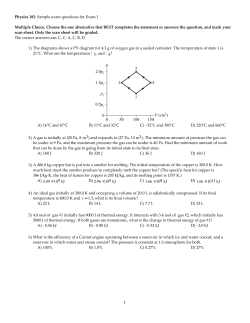
© Copyright 2026