
A Field Experiment on Effort Allocation under Relative Grading
A Field Experiment on Effort Allocation under Relative
Grading
Andy Brownback
∗
University of California, San Diego
January 13, 2015
Abstract
Grading on the curve is one of the most commonly used evaluation mechanisms
in education. Under this mechanism, grades are assigned based on each student’s
percentile rank in the class. Considering classes to be samples from the population
implies that as the class size grows, the percentile ranks of the students in it draw closer
to their percentile ranks in the population, which changes the students’ incentives. I
model this environment to predict how changes in the class size reallocate incentives for
effort between students with different abilities, an effect that holds true in any relative
evaluation method. I use a field experiment in an intermediate economics course to test
the model’s predictions about effort exertion in a real-stakes environment. My results
show that the lower variance of larger classes elicits greater mean effort and greater
effort from all but the lowest-ability students. The greater variance of smaller classes
elicits more effort from only the lowest-ability students. Many low-ability students fail
to take advantage of the randomness of the smaller class size, an allocation failure
consistent with “cursed” beliefs about their classmates and other behavioral biases.
My results shed new light on the debate over the effects of class size reductions.
∗
Department of Economics, UCSD, La Jolla, CA 92093, [email protected]. I would like to thank
James Andreoni for his careful guidance and incredible support. Additional thanks are due to Prashant
Bharadwaj, Simone Galperti, Laura Gee, Uri Gneezy, Michael Kuhn, Paul Niehaus, Marta Serra-Garcia,
Joel Sobel, Charles Sprenger, Isabel Trevino, and Joel Watson.
1
1
Introduction
Relative evaluation mechanisms are frequently used to mitigate the effects of asymmetric
information between a mechanism designer and economic agents. Designers with incomplete
information about agents’ costs and valuations may prefer to employ relative evaluation
mechanisms in which agents compete away much of each others’ surpluses, since a poorly
calibrated absolute mechanism offers little incentive for effort.
Consider, for example, a teacher who wishes to maximize effort from his students. Setting
an absolute threshold for each grade that is too high or too low could cause students to exert
minimal effort. This teacher may remedy his incomplete information about his students’
abilities by grading on the curve. Under a relative or “curved” grading mechanism, the
evaluation of a student’s performance is based on her percentile rank within her comparison
group independent of any absolute measure of her performance. These mechanisms have become a fixture in many university classrooms and law schools.1 Indeed, mechanism designers
across many areas of education employ relative evaluation in competitions for scholarships,
college admissions, and even teacher pay.2,3,4
Under relative evaluation, the composition of an agent’s comparison group is critical in
determining the agent’s outcome at a given level of effort. I refer to a sample drawn from
the population into a comparison group as a “cohort.” The law of large numbers implies
that the larger this cohort becomes, the more it comes to resemble the distribution from
which it is drawn. Since the composition of a cohort determines the incentives for effort by
an agent, the size of a cohort affects those incentives by bringing its expected composition
closer to the population distribution. Therefore, in theory, the incentives for effort under any
1
Mroch (2005) estimates that 79% of law schools standardize scores according to a grading curve.
Missouri’s Bright Flight scholarship program awards scholarships to the top 3% of high school seniors
based on ACT or SAT scores.
3
In California, the top 9% of graduating seniors are guaranteed admission to one of the University of
California campuses. In Kansas, the top 33% are guaranteed admission to the state college of their choice.
In Texas, the top 10% are offered similar incentives.
4
North Carolina Senate Bill 402 section 9.6(g) grants favorable contracts to the top 25% of teachers at
each school as evaluated by the school’s administration.
2
2
relative evaluation mechanism can be modeled and understood as a function of cohort size.
A mechanism designer concerned about the allocation of incentives to agents could equalize
incentives across any two cohort sizes by manipulating the number or value of prizes awarded.
In practice, however, mechanism designers typically operate under constraints restricting
them to a given number or percentage of prizes awarded regardless of cohort size. For
example, a professor may be obligated to award A’s to 20 percent of his students. This
paper evaluates the theoretical and empirical effect of cohort size on incentives for effort in
a relative evaluation mechanism under such a constraint.
Consider an example, Texas HB 588 grants automatic admission to any Texas state
university—including the University of Texas at Austin—to all Texas high school seniors
who graduate in the top 10 percent of their high school class.5 Each graduating class is
therefore subject to a distinct relative evaluation mechanism under the restriction that each
mechanism must award 10 percent of the students automatic admission, regardless of the
class size. Since Texas high schools vary in size by orders of magnitude,6 the law of large
numbers implies that the incentives for effort under this policy will vary dramatically by
school. Smaller high schools are more likely to draw graduating classes full of outliers, adding
uncertainty around the returns to effort, while cohorts of students in larger high schools are
more likely to reflect the characteristics of the population, reducing the uncertainty around
the returns to effort.
While the theory clearly indicates that incentives change with the size of a cohort, whether
students identify and react to these incentives is uncertain. Prior research casts doubt on
the ability of economic agents to draw accurate inference about information that depends
critically on sample size (Tversky and Kahneman, 1971; Kahneman and Tversky, 1973;
Rabin, 2002; Benjamin, Rabin, and Raymond, 2014). Therefore, research is necessary to
uncover the reactions of agents to these changing incentives.
5
The bill was modified in 2009 to stipulate that the University of Texas at Austin may cap the number
of students admitted under this measure to 75% of in-state freshman students.
6
Plano East High School has an enrollment of 6,015 students, while Valentine High School has an
enrollment of 9 students.
3
This paper presents the results of a field experiment on relative grading in a large, upperdivision economics course at the University of California, San Diego (UCSD) testing the
sensitivity of student effort to cohort size. I use an experimental intervention in the size of
a cohort to test its causal effect on effort by students who are graded on the curve. In order
to provide the most powerful test of this effect, I present students with a pair of quizzes
subject to an identical grading curve where the top 70 percent of scores in a cohort receive
high grades. Each week, for each student, I randomly determine which quiz in the pair will
be graded relative to a 10 student cohort and which will be graded relative to a 100 student
cohort. Since cohort size is randomly assigned to quizzes, I will refer to these as the “10Student Quiz” and the “100-Student Quiz.” I measure effort as the time a student spends
on a given quiz.
By comparing a pair of quizzes taken in quick succession but with different cohort sizes,
I can use the difference in the amount of time spent on each quiz to measure the causal
impact of cohort size on effort within a given student, within a time period. This cleanly
identifies student responses to changes in their strategic setting independent of any potential
classroom-specific, student-specific, or time-specific confounds that can plague classroom
studies.
In order to generate predictions about the ways in which a student subject to curved
grading would respond to changes in the cohort size, I develop a theoretical model of strategic
effort exertion in the classroom. Strategic concerns are just one of countless motivations a
student may have to exert effort in the classroom. My results uncover the relevance of these
other motivations per se and confirm that my experimental design has eliminated all of
these potentially confounding factors. I therefore abstract away from any other motivation
for effort and develop predictions based on expected-grade maximizing responses to the
underlying strategic incentives of the curved grading environment. In this simplified model,
I make several assumptions about students’ utility functions, their beliefs about their ability
relative to their classmates, their responses to those beliefs, and the separability of their cost
4
functions. As such, the value of this model is in generating qualitative predictions about the
allocation of effort by strategic students responding to a change in the size of their grading
cohorts. Indeed, from a policy perspective, it is the empirical effect of the cohort size on
effort allocation that is paramount. Confirming or rejecting a given model of strategic effort
will always be a secondary concern.
My model predicts that mean effort will increase with the size of the cohort. As the cohort
size grows and the characteristics of the cohort draw closer to the population characteristics,
the uncertainty surrounding the returns to any given level of effort decrease, drawing up the
mean effort.
My model also provides structure for how incentives differ by ability level. In particular,
incentives diverge on either side of the the 30th percentile of scores, where high and low grades
are separated. I refer to the quantile that distinguishes the two outcomes as the “cutoff.”
The 10-student cohorts have higher variance, increasing the marginal benefit of effort for
students with abilities below the cutoff. With lower variance, the 100-Student Quiz increases
the marginal benefit of effort for students with abilities above the cutoff. Thus, my model
predicts that “low-ability” students—those with GPAs below the 30th percentile—will exert
more effort on the 10-Student Quiz, and “high-ability” students—those with GPAs above the
30th percentile—will exert more effort on the 100-Student Quiz. These heterogeneous effects
highlight the tradeoffs between mean effort and the distribution of effort, a key tension for
optimizing classroom design.
My experimental results confirm the prediction that the mean effort will increase in
the cohort size. The 100-Student Quizzes elicit 5 percent more effort than the 10-Student
Quizzes, and this difference is significant at the 1 percent level. Next, I use GPA as a
proxy for ability in order to test my model’s predictions about the heterogeneous impact of
cohort size on students with different abilities. I first confirm that high-ability students exert
significantly greater effort on the 100-Student Quiz. My experimental results then deviate
from the model’s predictions in an important way. While the lowest ability students exert
5
more effort on the 10-Student Quizzes, this effect is not found for all students below the
cutoff. In fact, mean effort by students below the cutoff is higher on 100-Student Quizzes.
For these students, allocating greater effort to the 100-Student Quiz fails to take advantage of
the higher variance of the smaller cohorts. These deviations from the theoretical predictions
highlight the limits to the predictive ability of a purely strategic model of classroom effort.
Specifically, a strategic model under classical assumptions about beliefs and best responses
will overstate the distributional costs of increasing mean effort. That is, effort from lowability students is less negatively affected by increasing cohort sizes than theory predicts.
I attempt to uncover the origin of the misallocation of effort by low-ability students by
exploring the critical assumption that students hold accurate beliefs about their own ability
relative to the distribution of abilities among their classmates. A violation of this assumption
will cause the perceived incentives to deviate from the incentives the model predicts. For
this assumption to hold, students must forecast their distribution of classmates taking into
account the fact that higher ability students are more likely to enroll in upper-division
economics courses. “Cursed” students (Eyster and Rabin, 2005), on the other hand, may
wrongly perceive that the distribution of students in the class is simply an “average” draw
from the undergraduate population similar to the draws they faced in previous lower-division
courses. In order to examine the predictions of my model under cursed beliefs, I construct
a distribution of classmates using public data on grades from from lower-division UCSD
courses. My results show that the observed behavior of students is closer to the expected
behavior for students who best respond to cursed beliefs that fail to account for selection
into the course.
My results suggest that cursed beliefs are not the only potential complication in evaluating strategic effort exertion. Allowing for “fully cursed” beliefs7 shifts the predicted single
crossing point towards lower abilities and increases the number of students predicted to exert greater effort on the 100-Student Quiz but still cannot explain the behavior of many
7
Under cursedness, there are degrees to which agents infer information from other agents’ actions. A
fully-cursed agent draws no inference from the actions–in this case, enrollment decisions–of any other agent.
6
low-ability students. The misallocation of effort by these students is consistent with several
possible behavioral biases, among them, overconfidence, updating failures, and reference dependence. My experiment cannot independently identify these possible behavioral responses,
but I discuss the impacts of each and outline experiments that could identify the extent to
which each is responsible for deviations from the theoretical predictions.
My data can cleanly reject several alternative explanations for student behavior. A
model where high-ability students have greater intrinsic motivation provides some similar
predictions about how incentives for effort evolve with student ability and may be present as
an incentive for effort. Importantly, my experiment controls for this with its within-student
analysis. Therefore, without allowing for sensitivity to the strategic incentives present, this
model cannot generate the patterns of effort observed in my experiment. In a similar way, my
data can reject the notion that risk preference or demographic characteristics can explain
the results entirely. I can also reject the hypothesis that effort allocation is driven by a
correlation between GPA and the ability to intuit the incentives of the environment. Indeed,
my paper provides clean evidence that students respond strategically and systematically to
changes in the size of their grading cohorts, despite many other observable and unobservable
motivations for effort.
To fix ideas, I refer to grading mechanisms throughout this paper, but this should not distract from the generality of the results. Relative awarding mechanisms are found throughout
the modern economy in job promotion contests, performance bonuses, and lobbying contests,
among others.8 Since the costs of effort, the means of exerting it, and the ways in which
heterogeneous abilities manifest themselves are all similar in academic and professional settings, my results provide a framework for predicting how certain mechanisms will affect the
allocation of effort across employees.
The outline of this paper is as follows. In Section 2, I provide a survey of the relevant
8
For example, in his book Straight from the Gut, former GE CEO Jack Welch recommends that managers
rank employees according to a 20-70-10 model of employee vitality where 20% of employees are labeled “A”
players, 70% “B” players, and 10% “C” players. “A” players are rewarded, and “C” players are eliminated.
7
literature. In Section 3, I outline a simple model of incentives under relative grading. This
model yields qualitative predictions that I test experimentally. The experiment itself is
formally introduced in Section 4. Section 5 presents the results of the experiment and tests
the predictions of the model, addressing several alternatives to my model including cursed
beliefs. Section 6 discusses the results. Section 7 concludes the paper.
2
Literature
In addressing the strategic incentives of classroom grading mechanisms, this paper spans
three distinct literatures: experimental economics, microeconomic theory, and the economics
of education. In the realm of experimental economics, it owes a debt to many prior experimental tests of contests and auctions. My model has roots in a long theoretical literature
on contests. Notably, Becker and Rosen (1992), who modify the tournament structure of
Lazear and Rosen (1981) to generate predictions for student effort under relative or absolute
grading mechanisms. By modeling and collecting data in a classroom setting, my paper contributes to a literature on classroom performance that has been explored in the economics
of education.
Experiments testing effort exertion in different laboratory settings date back to Bull,
Schotter and Weigelt (1987), who test bidding in laboratory rank-order tournaments. They
find that bidders approach equilibrium after several rounds of learning. Equilibrium behavior
in laboratory all-pay auctions is more elusive with the majority of studies demonstrating
overbidding (Potters, de Vries, and van Winden, 1998; Davis and Reilly, 1998; Gneezy and
Smorodinsky, 2006; Barut, Kovenock, and Noussair, 2002). Müeller and Schotter (2010) and
Noussair and Silver (2006) confirm the overbidding result, but also uncover heterogeneous
effects for different types of bidders. For an exhaustive survey of the experimental literature
on contests and auctions, refer to Dechenaux, Kovenock, and Sheremeta (2012).
Andreoni and Brownback (2014) provide a framework for evaluating the effects of contest
8
size on bids in a laboratory all-pay auction along with the first directed test of the independent effect of contest size on effort. Larger contests in this setting are found to generate
greater aggregate bidding, greater bidding by high types, and lower bidding by low types.
Other studies that find effects of contest size on effort restrict their focus either to small
changes in the size of contest (Harbring and Irlenbusch, 2005) or changes that also affect the
proportion of winners (Gneezy and Smorodinsky, 2006; Müeller and Schotter, 2010; Barut
et al., 2002, List et al., 2014).
This paper takes the framework of Andreoni and Brownback (2014) out of the laboratory
and into a field setting and is, to my knowledge, the only study that directly measures effort
as a function of the classroom size. Classroom experiments have been conducted to answer
other questions. The state of Tennessee experimented with classroom sizes for kindergarten
students (Mosteller, 1995), but student outcomes, not inputs, were the focus of the study
and the setting was non-strategic. Studies have also explored the responsiveness of effort
to mandatory attendance policies (Chen and Lin, 2008; Dobkin, Gil, and Marion, 2010) or
different grading policies (Czibor et al., 2014), finding mixed results. I explicitly control for
factors related to classroom instruction or procedures in order to uncover the direct effect of
changes in the strategic incentives for effort.
In the microeconomic theory literature, the study of contests was originally motivated
by the study of rent-seeking (Tullock, 1967; Krueger, 1974), but has since evolved into a
more general branch of research that considers various environments with costly effort and
uncertain payoffs. The three models most often employed are the all-pay auction (Hirshleifer
and Riley, 1978; Hillman and Samet, 1987; Hillman and Riley, 1989), the Tullock contest
(Tullock, 1980), and the rank-order tournament (Lazear and Rosen, 1981).
Hillman and Riley (1989) and Baye, Kovenock, and de Vries (1993) use the all-pay
auction model to explore the incentives for rent-seeking in politics. Amann and Leininger
(1996) introduce incomplete information about opponents’ types to generate a pure-strategy
equilibrium bidding function. Baye, Kovenock, and de Vries (1996) fully characterize the
9
equilibrium of the all-pay auction and demonstrate that a continuum of equilibria exist.
Moldovanu and Sela (2001) develop a model of optimal contest architecture for designers
with different objectives. For a comprehensive theoretical characterization of all-pay contests
that incorporates many of the existing models into one framework, see Siegel (2009).
This paper is motivated by the way in which the size of a contest changes the incentives for participants. Moldovanu and Sela (2006) capture this intuition more generally and
demonstrate the single-crossing property of symmetric equilibria in differently sized contests. Olszewski and Siegel (2013) provide similar results about equilibria in a general class
of contests with a large but finite number of participants.
My paper considers strategic interactions between students, unlike much of the previous
work on grading mechanisms. The contest-like relative grading mechanisms as well as absolute grading mechanisms are often studied in the economics of education. Costrell (1994)
explores the endogenous selection of grading standards by policy makers seeking to maximize social welfare, subject to students who best respond to those standards. Betts (1998)
expands this framework to include heterogeneous students. Betts and Grogger (2003) then
look at the impact of grading standards on the distribution of students.
Both Paredes (2012) and Dubey and Geanakoplos (2010) compare incentive across different methods of awarding grades. The former considers a switch from an absolute to a relative
grading mechanism, while the latter finds the optimal coarseness of the grades reported when
students gain utility from their relative rank in the class.
The education literature traditionally studies class size like an input to the production
function. The aforementioned Mosteller (1995) paper operates in this vein, finding that
the decrease in class size caused by the Tennessee class size project had lasting impacts on
the outcomes of students. Kokkelenberg, Dillon, and Christy (2008) find a negative effect
of class size on the grades awarded to individual students in a non-strategic environment.
The independent effect of class size on strategically interacting students, however, remains
unstudied. Contest size is often taken as given or assumed to be determined exogenously. In
10
this paper, I demonstrate that cohort size plays a significant role in a student’s selection of
effort when grading on the curve. Thus, a classroom designer optimizing student outcomes
needs to take into consideration the heterogeneous effects of cohort size on students with
different abilities.
3
A Model of Academic Effort
In this section I develop a simple framework outlining the incentives for effort present when
grades are awarded on a relative basis. This model will provide generic predictions about
the direction a strategic student should shift effort as the cohort size changes. Providing
a formalization of the way student incentives are tied to cohort size will be instructive for
building intuition and developing ways to test whether students view the classroom as a
strategic environment and if they predictably respond to shifts in strategic incentives.
Strategic incentives will be present amidst myriad other incentives for effort. As such, the
contribution of this model is in the structure that it gives to the relative incentives for effort,
not the point estimates it provides for the amount of effort each student chooses. Focusing
on the relative incentives for effort provides predictions independent of other motivations for
effort, better matching my experiment, which explicitly controls for alternative motivations.
The heterogeneity this model predicts relies on several assumptions about the beliefs and
information that each student has. In section 6, I discuss the model’s dependence on these
assumptions and the way predictions change when they are relaxed.
In solving this model, I borrow heavily from the independent private value auction (Vickrey, 1961) and the all-pay auction literatures (Baye, Kovenock, and de Vries, 1993). Suppose
there are N students exerting costly effort in order to increase their chances of winning one
of M ≡ P × N prizes in the form of high grades. Effort appears as scores on quizzes, and
high grades are awarded to the students with the highest M scores.
Suppose each student has an ability, ai , distributed uniformly from 0 to 1. That is
11
ai ∼ U [0, 1], meaning F (ai ) = ai . Students are evaluated at each period, t, based on their
academic output, or “score,” si,t from that period. Suppose that scores have a constant
marginal cost that is inversely related to ability,9
C (si,t ; ai ) =
3.1
si,t
.
ai
(1)
Student’s Utility
The expected utility of a student is determined by both the likelihood of receiving a high
grade at a given score and the cost of that score. Normalize the value of receiving a high
grade to one. Heterogeneity across students with different ability levels is now captured by
the cost of generating a given score. Thus, a student’s utility is given by
U (si,t ; ai ) = Pr si,t ≥ S¯ −
si,t
,
ai
(2)
where S¯ represents the minimum score required to receive a high grade.
I restrict my attention to the set of functions, S : (ai ; N, P ) 7→ si,t , that take parameters,
N and P , and map abilities to scores in such a way as to constitute a symmetric equilibrium
of the model. In the appendix, I prove that any such function must be monotonic in ability.
In addition to monotonicity, it is straightforward to show that scores must also be continuous
in ability.10 All continuous, monotonic functions are invertible, so there exists a function that
maps a given score back onto the ability implied by that score. Given that the equilibrium
scores depend on the parameters, N and P , this inverse function, too, depends on these
parameters. I define the function A(si,t ; N, P ) ≡ S −1 (si,t ; N, P ).
With invertibility established, the probability of receiving a high grade is equivalent to
9
The actual value of the marginal cost will not be critical as my within-subjects experimental design
controls for student-specific costs of effort.
10
Suppose not. With discontinuities within the support of S(ai ; N, P ), some students would be failing to
best respond. A student scoring just above the discontinuity would be able to increase his expected utility
by lowering his score, which would lower his costs, up until the discontinuity in scores has vanished.
12
the probability that the ability level implied by a student’s score is higher than the ability
levels implied by the scores of N − M other students. At equilibrium, this probability is
represented as an order statistic giving the probability that a student’s ability is among the
top M abilities of her cohort. Substituting in the experimental parameters, N = {10, 100}
0
Probability that Ability is in the Top 70%
.2
.4
.6
.8
1
and P = 0.7, yields the order statistics presented in Figure 1.
0
.2
.4
.6
.8
1
Ability
N=10
N=100
Figure 1: Probability a Given Ability is in the Top 70% of Abilities in a Cohort of Size N
Figure 1 reveals the key intuition of this paper. For low-ability students, the uncertainty
of the 10-Student Quiz increases their likelihood of encountering cohorts in which they are
among the top 70 percent. For high-ability students, that same uncertainty decreases the
likelihood that they are among the top 70 percent of their cohort. These probabilities
heterogeneously vary the expected returns to student effort.
13
Plugging the order statistics into (2) completes the student’s utility function.
U (si,t ; ai , N, P ) =
N
−1
X
!
j=N −N P
(N − 1)!
A(si,t ; N, P )j
j!(N − 1 − j)!
× (1 − A(si,t ; N, P ))N −1−j −
si,t
.
ai
(3)
In the appendix, I solve for the equilibrium scores as a function of ability. Figure 2 plots
the equilibrium score functions at the experimental parameter values, N = {10, 100}. It is
worth noting that the point estimates represented are not valuable per se, as my predictions
0
Symmetric Equilibrium Score
.1
.2
.3
relate to relative, not absolute scores.
0
.2
.4
.6
.8
1
Ability
N=10
N=100
Figure 2: Scores at Equilibrium in the 10- and 100-Student Quizzes
While the function mapping the ability of a student to his or her score at equilibrium
is clearly quite complicated, the intuition behind it is rather simple. low-ability students
14
benefit from the introduction of randomness into the draw of their cohort, and put forth
greater effort. Conversely, randomness is detrimental to high-ability students, so their effort
decreases.
A thought experiment can reveal the intuition behind the equilibrium score functions in
more depth. Consider the symmetric best response function in an environment where the
proportion of winners remains constant at P = 0.7, but the number of students in a cohort
approaches infinity. The law of large numbers ensures that the distribution of students in
the cohort approaches a perfect reflection of the probability distribution from which they are
drawn. Thus, common knowledge of the probability distribution is sufficient for a student’s
belief about her relative position in her cohort to approach certainty.
In this infinitely large cohort, a student whose ability is greater than the 30th percentile
in the probability distribution will best respond by choosing a score that no student below
the 30th percentile can match and receive non-negative expected surplus. That score, given
the assumed cost function, is approximately si,t = 0.3.11 Students below the 30th percentile
best respond with a score of si,t = 0. Thus, the equilibrium score function in this setting
approaches a step function.12
Keeping in mind the limiting case, consider the equilibrium scores in Figure 2. Deviations
from the infinite case can be explained through marginal benefits and marginal costs. For
students who choose si,t > 0 in the limiting case, the marginal benefit of lowering a score is
constant and identical across treatments—scores have a constant marginal cost, so foregone
scores have a constant marginal benefit. The marginal cost of lowering a score is paid
through reductions in the probability of receiving a high grade. In the 10-Student Quiz, that
probability changes more gradually, making marginal reductions of scores less costly, casing
the 10-Student Quiz scores to drop below the 100-Student Quiz scores.
11
This value itself means little except as an ordinal measure of academic output.
To be precise, the rules of this environment need to change to accommodate the fact that students have
a probability measure of 0 in an infinitely large contest. One option is to begin by awarding a prize to the
student with the highest score and continue awarding prizes to students in decreasing order of score until 70
percent of students have been awarded prizes. Thus, there is no profitable deviation where a student earns
a prize with a score of si,t = 12
15
Now consider students with si,t = 0 in the infinitely sized cohort. Increasing scores
bears a constant marginal cost for both the 10- and 100-Student Quizzes, but holds a higher
marginal benefit in the 10-Student Quiz because the randomness increases the likelihood of
states of the world in which low scores receive high grades. So, the 10-Student Quiz scores
rise above the 100-Student Quiz scores.
3.2
Predictions From the Model
My experiment pairs 10- and 100-Student Quizzes each week, and my analysis takes the
difference in effort between the two quizzes—specifically, the 100-Student Quiz duration
minus the 10-Student Quiz duration—as its dependent variable. I refer to this difference
as the “treatment effect.” I use the model’s predictions for the difference in scores as a
proxy for its predictions about the difference in effort. This allows me to remain agnostic
about the production function for scores, only assuming that higher predicted scores imply
higher predicted effort. My within-subjects analysis of this difference in effort controls for
student-specific heterogeneity in costs of production and will provide a cleaner test of the
treatment effect. To see the model’s predictions for how the treatment effect will evolve with
ability consider Figure 3, which plots the equilibrium score in the 100-Student Quiz minus
the equilibrium score in the 10-Student Quiz as a function of ability.
The model provides three primary predictions about the treatment effect displayed in
Figure 3. While the point estimates of the model are based on specific assumptions, the
following predictions represent generic qualities that provide clarity about the ways in which
an expected-grade maximizing student may react to changes in the grading environment.13
Hypothesis 1: Mean effort is increasing in cohort size.
My model predicts that the greater effort exerted by high-ability students on the 100-Student
Quiz outweighs the greater effort that low-ability students exert on the 10-Student Quiz,
13
Moldovanu and Sela (2006) prove these properties for a general class of cost functions. These predictions
derive from a single-crossing property they prove for symmetric equilibria in contests with different N but
fixed P .
16
100-St. Quiz Score Minus 10-St. Quiz Score
-.05
0
.05
.1
0
.2
.4
.6
.8
1
Ability
Figure 3: Difference in Score between 100- and 10-Student Quizzes at Equilibrium
causing average effort to increase in cohort size.
Hypothesis 2: The treatment is negative for low-ability students.
Hypothesis 3: The treatment is positive for high-ability students.
My model predicts that the treatment effect begins negative and moves positive, crossing
the horizontal axis exactly once. Call this single-crossing point a∗ . Based on Figure 1, it is
natural to think of a∗ as corresponding with the cutoff. This is approximately true, but the
specific location of a∗ will depend on the distribution of abilities, and the cost function for
scores. My predictions focus on the cutoff of ai = 0.3 as a∗ .14
14
While the single-crossing point in Figure 3 is not precisely 0.3, the salience of the 30th percentile in my
experiment and the proximity of the single-crossing point to this value make it a natural candidate.
17
4
Experimental Design
My experiment takes the paired-auction design used in Andreoni and Brownback (2014) and
adapts it for a classroom context. My design simultaneously presents students with a pair of
quizzes, a 10-Student Quiz and a 100-Student Quiz, and records student behavior on each.
This design is inspired by the paired auction design of Kagel and Levin (1993) and Andreoni,
Che, and Kim (2007).
I analyze the difference in behavior between the two simultaneous quizzes in order to
control for student-specific and week-specific effects. This paired design will provide a powerful test of responses to cohort size that occur in the classroom, an environment riddled
with alternative motivations for effort.
4.1
Recruitment and Participation
The experiment was conducted in the winter quarter of 2014 in an intermediate microeconomics course at UCSD. Enrollment in the course started at 592 students, and ended at 563
after some students withdrew from the course. All enrolled students agreed to participate in
the experiment. The experiment was announced both verbally and via web announcement
at the beginning of the course. The announcement can be found in the appendix.
4.2
Quiz Design, Scoring, and Randomization
There were five Quiz Weeks in the quarter. At noon on Thursday of each Quiz Week, two
different quizzes covering material from the previous week were posted to the course website.
Both quizzes were due by 5pm the following day. Each quiz consisted of four questions and
had a time limit of 30 minutes. The 30-minute limit ensures that the quiz was given focused
attention with little time spent idle, meaning that the time recorded for students is reflective
of their effort on the quizzes. Students could take the quizzes in any order.
I refer to the content of the two quizzes in a pair as “Quiz A” and “Quiz B.” The two
18
quizzes were presented to students in the same order, but I randomly assigned grading
treatments to each. One of the quizzes received the 10-Student Quiz treatment and one
received the 100-Student Quiz treatment. Therefore, while every student was assigned both
Quizzes A and B, approximately half of them had Quiz A graded as the 10-Student Quiz and
half had it graded as the 100-Student Quiz. The opposite treatment was assigned to Quiz
B in each case. The questions on Quizzes A and B were designed to have as little overlap
as possible to eliminate order effects in effort or scores. Before beginning the quiz, students
only observed the grading treatment, and not the quiz content. No student was informed of
the treatments received other students. Table 1 shows the balance across treatments.
Table 1: Submitted Quizzes from Each Week and Each Treatment
Quiz Version
A
B
Treatment Week 1 Week 2 Week 3 Week 4 Week 5
10-Student
201
282
258
253
249
100-Student
262
282
259
253
243
10-Student
267
280
262
251
243
100-Student
200
282
259
256
252
Note: Asymmetries across treatments may arise out of chance, failed submissions, or
withdrawals. Asymmetries in completion rates will not affect the analysis, since only
completed pairs will be analyzed.
The number of questions correct determined the score for each student. The top 7
scores received high grades in each 10-Student Quiz cohort, and the top 70 scores received
high grades in each 100-Student Quiz cohort. Students were informed that they would be
anonymously re-randomized into cohorts each week. Cohorts consisted of students who had
taken the same quiz under the same grading treatment. Students receiving high grades were
awarded 3 points, while students receiving low grades were awarded 1. Non-participants
received 0 points. The quizzes counted for approximately 13 percent of the total grade in
the class, providing strong incentives for effort. Students whose scores were tied at the
70th percentile of a cohort were all awarded 3 points unless the tied students all failed to
participate, in which case the students all received 0 points.
19
4.3
Effort
The time at which every quiz was started and completed was recorded to the millisecond. My
analysis will take the amount of time that a student spent taking a quiz to be the measure
of effort that the student exerted on that quiz. This measure of effort will reveal which quiz
the student believed to hold the greater returns to her effort.
Both quizzes were posted simultaneously, meaning that the amount of time a student
could spend studying prior to starting either quiz was roughly constant between the two
quizzes. Student behavior supports this assertion. 86 percent of students waited less than
an hour between the two quizzes, with a median interval of 32 minutes.
4.4
Ability
At the beginning of the course, students consented to the use of their grade point average
(GPA) in this study.15 I use this as the measure of academic ability in the analysis. I elected
not to use exam performance in the course because of the endogeneity between the allocation
of effort to exams and quizzes. I contend that GPA is a more valid instrument for ability
because, unlike exams, there is no sense in which quiz effort and GPA are substitutable.
While there may be a correlation between the level of effort and ability as measured by
GPA, my analysis will eliminate these level effects by only considering differences in effort
between pairs of quizzes.
Figure 4 shows the cumulative distribution function of all student GPAs in the class. I
use the value of the cumulative distribution function at a given GPA to represent the ability
level of that student in my predictions. Importantly, the GPA at the 30th percentile is 2.72.
The median and mean GPA are 3 and 2.99, respectively. Seven students have a GPA of 4.0,
while only one student has the minimum GPA of 1.0.
15
Due to administrative delays, I was not able to get a student’s GPA until after the quarter. Thus, the
response to the treatment will have some impact on ability. Since the quizzes only amounted to approximately
13 percent of the students grade in one of dozens of classes they have taken, I do not see this as a major
problem.
20
99
Percentile Rank in Class
30 40
60
80
20
0
1
2
2.72
3
4
GPA
Figure 4: Cumulative Distribution Function for GPAs of All Students in the Experiment
5
Results
I begin this section by describing my data and their basic statistics. Then, I specify the
dependent variable I will use in the analysis and test its aggregate characteristics. Next, I
demonstrate heterogeneous treatment effects across students of different ability levels and
test where the model does and does not hold predictive power. Finally, I investigate possible
explanations for the model’s failures.
5.1
Data and Descriptive Statistics
In total, 579 students submitted 5,094 online quizzes in this experiment. Of those, 2,546 had
been assigned to a 10-Student Quiz, and 2,548 had been assigned to a 100-Student Quiz.
The duration of each quiz was recorded, and my analysis will include every recorded time
21
appearing in a completed pair of quizzes. Table 2 reports the means and standard deviations
of the quiz durations for both cohort sizes.16
Table 2: Descriptive Statistics on the Duration of the Quizzes
100-Std. Quiz 10-Std. Quiz
Mean Duration (in minutes)
14.97
14.58
Standard Deviation/Error
(9.21)
(9.00)
Note: In this table, the quiz means are unpaired, so will provide a
much weaker test of significant differences.
5.2
Dependent Variable
My analysis uses the difference between the time allocated to the 100- and 10-Student Quizzes
as the dependent variable. Recall that I refer to this difference as the treatment effect. This
dependent variable is appealing because it reveals a student’s beliefs about which quiz will
yield higher returns to her effort. Since random assignment leaves effort costs and quiz
difficulty independent of the cohort size, if a student shows a general trend toward spending
more time on the 10- or 100-Student Quiz, then the student must believe that her marginal
product is higher on that quiz.17 Using within-student differences also offers the best control
for individual-specific and week-specific noise in the data.
16
Since I did not receive GPA data until the end of the quarter, I was not able to observe the GPAs of
the students who dropped during the quarter. There were only 20 submitted pairs of quizzes from students
who dropped the course. The mean treatment effect for these quizzes is approximately -36.7 seconds with
a standard deviation of 432 seconds. I include these data in the analysis of the mean treatment effect, but
exclude them from the analysis of heterogeneity in treatment effects, since I have no measure of ability. Each
of these decisions biases my results away from the model’s predictions. For the means, it lowers the average
effect, diminishing my results. With respect to heterogeneity, their inclusion only strengthens my results,
because they are more likely to be low GPA students, and their average treatment effect is negative.
17
Since I only include times recorded in a completed pair of quizzes, my analysis reveals the perceived
relative returns to effort conditional on participation in both quizzes. The results do not substantively change
by replacing all skipped quizzes with values of 0, but the standard errors expand, as 0 is a much shorter
duration than any observed in the data.
22
5.3
Endogenous Selection and Controls
One potential complication in these results is that the order of quiz completion could not
be controlled and thus is endogenous.18 Fortunately, even though quizzes are presented simultaneously, one quiz is positioned above the other vertically. The presentation order of
treatments is randomly assigned and provides a relevant instrument for the order of completion that is mechanically designed to be valid. The effect of this endogenous selection is
not large–51.4 percent of 100-Student Quizzes were presented first online, while 55.3 percent
were completed first–but is statistically significant.
Column 1 of Table 3 demonstrates that the instrument is extremely relevant. Column 2
shows that the instrument has a problematic correlation with student GPA. Despite being
randomly assigned before each Quiz Week, the order in which the quizzes were presented
happened to correlate to the GPAs of the students. This is unfortunate but was unavoidable,
since I did not have access to student GPAs until the end of the quarter. Additionally, the
explanatory power is minimal, with an R2 value below 0.002. Column 3 demonstrates that
the residual effect of GPA on the order in which a student completes the quizzes has negligible
explanatory power and is not statistically significant after controlling for presentation order.
To demonstrate that endogenous selection does not drive any results, all tables will feature
results with and without the instrument for quiz completion order.
Hypothesis 1: Mean effort is increasing in cohort size.
Table 4 tests my model’s straightforward prediction that mean effort is increasing in the
cohort size. Column 1 shows that, on average, students spend approximately 27 more seconds
on the 100-Student Quiz than on the 10-Student Quiz, an increase of 3 percent over the
mean. With endogenous selection of ordering, however, this number is confounded by the
effect of quiz order on quiz duration. Instrumenting for the order of completion removes
this endogeneity and provides a clearer picture of the treatment effect, showing that the
18
This is a limitation of the online environment. In order to force students to take quizzes in a specific
order the second quiz must be hidden from view until the completion of the first quiz. I posted both quizzes
simultaneously in order to ensure that students knew they were assigned two quizzes.
23
Table 3: Testing the Relevance and Validity of the Instrument
100-St. Quiz
presented first
GPA
Constant
R2
N
(1)
(2)
Pr{100-St. Quiz Pr{100-St. Quiz
completed first} presented first}
0.759***
(0.05)
0.105**
(0.05)
-0.243***
-0.290**
(0.04)
(0.14)
0.064
0.002
2,486
2,486
(3)
Pr{100-St. Quiz
completed first}
0.757***
(0.05)
0.060
(0.05)
-0.422***
(0.15)
0.065
2,486
* p<0.10, ** p<0.05, *** p<0.01
Note: The first column demonstrates that the order in which quizzes are displayed is a
highly relevant instrument for the order in which the quizzes are completed. The second
column shows the troubling correlation that the mechanically random instrument has with
the GPAs of students, though the explanatory power is negligible. The third column shows
that the relevance of the instrument is not a result of its correlation with GPA.
100-Student Quiz elicits 46.4 seconds more effort from students, an increase of more than 5
percent over the mean.19
Table 4: Mean Difference between 100- and 10-Student Quiz Duration
OLS
100-St. Quiz
Taken First
Constant
Instrumented
N
0.450**
(0.19)
No
2,507
IV Regression
-6.085***
(1.25)
0.773***
(0.20)
Yes
2,507
* p<0.10, ** p<0.05, *** p<0.01
All values are reported in minutes.
All standard errors clustered at the student level.
Result 1: Mean effort is increasing in the cohort size.
19
Inserting direct controls for the order of completion is not a valid measure, since the endogenous order
of completion is collinear with the treatment effect.
24
5.4
Heterogeneity in the Treatment Effect
My model predicts heterogeneity in the treatment effect across ability levels. I test this in
two ways. I first address it semi-parametrically, testing the mean treatment effect within
low- and high-ability students. Second, I impose continuity on the treatment effect across
students with different abilities in order to understand how it evolves.
It is important to note that the complicating influence of other incentives for effort will be
most apparent when considering the heterogeneity of the treatment effect. Deviations from
the theory may manifest themselves through biased beliefs, correlations between intrinsic
motivation and GPA, heterogeneous comprehension of the strategic incentives, or correlations
between demographic characteristics and GPA. After testing the specific predictions of the
model, I address each of these in turn.
Hypothesis 2: The treatment is negative for low-ability students.
Hypothesis 3: The treatment is positive for high-ability students.
To semi-parametrically test the heterogeneity of treatment effect, I regress the treatment
effect on indicator variables for low- and high-ability students. The results are presented
in Table 5. The first column shows significant and positive treatment effects for low-ability
students and positive but insignificant treatment effects for high-ability students. Including
the instrument for the order of quiz completion more accurately characterizes the treatment
effect. In the second column, the treatment effect remains positive for low-and high-ability
students, but is now significant for both. These results reject Hypothesis 2 but confirm
Hypothesis 3.
This continuous evolution of the treatment effect will allow us to explore these heterogeneous effects in more detail. Figure 5 plots a locally linear polynomial smoothing function
estimate of the treatment effect along with 95 percent confidence intervals, providing an
empirical test of the predictions of Figure 3.20
20
I include a less parametric test of evolution of the treatment effect in the appendix, showing that the
results are not driven by the continuity restriction.
25
Table 5: Difference between 100- and 10-Student Quiz Duration by Ability
OLS
100-St. Quiz
Taken First
Low-Ability
GP A < 2.72
High-Ability
GP A ≥ 2.72
Instrumented
N
0.706**
(0.31)
0.348
(0.23)
No
2,507
IV Regression
-6.043***
(1.26)
0.954***
(0.32)
0.699***
(0.25)
Yes
2,507
* p<0.10, ** p<0.05, *** p<0.01
All values are reported in minutes.
All standard errors clustered at the student level.
Consider the evolution of the treatment effect beginning with the lowest-ability students.
The model predicts that these particularly weak students understand the futility of their
efforts and show no sensitivity to the treatment effects. In contrast to these predictions, the
left tail of the distribution of GPAs shows a significant negative treatment effect with the
minimum treatment effect occurring at the boundary, where the predicted change in effort is
-175.7 seconds. This tail represents just over 2 percent of the population, but is economically
significant, as policy makers regularly design policies around the interests of the most at-risk
students. For these students, changing from a 10- to 100-student cohort results in a 19.3
percent reduction in effort. This pattern is not consistent with the specific predictions of the
model but is consistent with the general intuition that weaker students benefit more from
the randomness of the 10-Student Quiz.
The treatment effect then crosses the axis and becomes significant and positive for the
remaining low-ability students. For the high-ability students, the treatment effect is positive,
but decreasing in GPA, returning to near-zero for the highest-ability students. Qualitatively,
this pattern is similar to what my model predicted—that the treatment effect would cross
the axis once and from below.
26
100-St. Quiz Time Minus 10-St. Quiz Time
-300
-200
-100
0
100
1
1.74
2
2.72
Student GPA
Local Polynomial Fit
3
4
95% Confidence Interval
Figure 5: Local Polynomial Fit of the Difference in Effort between 100- and 10-Student
Quizzes (Times Reported in Seconds)
While these tests support qualitative predictions of my model, they also suggest that
the model misses the mark with respect to specific locations of phenomena. Specifically, my
model makes a focused prediction that the treatment effect crosses from negative to positive
near the cutoff at the 30th percentile, or a GPA of approximately 2.72. Table 5 easily
rejects this location for the single-crossing point. Statistical testing fails to reject the null
hypothesis that the coefficient of the treatment effect is identical for low- and high-ability
students (F = 0.43 P = 0.512). In fact, the raw mean difference between the 100- and 10Student Quizzes below the cutoff is 44.4 seconds, a greater value than the mean difference
above the cutoff, 20.0 seconds.
Figure 5 provides a more specific test of the single-crossing point of the treatment effect.
27
The point at which the smoothing estimate crosses the horizontal axis is approximately a
GPA of 1.74, or the second percentile of student GPAs. For a more non-parametric estimate
of the single-crossing point, I first note that all differences in effort above the single-crossing
point should be positive, while all differences in effort below it should be negative. I then
use two measures to assess the fit of different possible single-crossing points. First, I find
the point that maximizes the absolute number of positive differences in effort above it and
negative differences in effort below it. My second measure finds the point that maximizes
the sum of the differences with the predicted sign minus the sum of the differences without
the predicted sign. Using both of these measures, the single-crossing point that best fits the
data occurs at a GPA of 1.81 or approximately the 3rd percentile.21
Result 2: Contrary to the predictions of the model, the mean treatment effect is positive for low-ability students. The lowest-ability students, however, show significant negative
treatment effects.
Result 3: As the model predicted, the treatment effect is positive for all high-ability
students.
5.5
Alternatives to the Neo-Classical Assumptions of the Model
Using my model as the backbone for understanding the patterns of effort allocation when
students are graded on the curve provides several qualitatively accurate predictions, but
understandably fails with regards to more focused predictions. Interactions between the
treatment effect and alternative motivations for effort could cause shifts in the locations of
specific phenomena but will nonetheless preserve the shape and single-crossing nature of the
treatment effect that the data show.
To the extent that my experimental results provide evidence on the effects of these
alternative motivations for effort, I address them below. Additional behavioral phenomena
may be present but are not identified by my data. I explore the implications of several of
21
In both cases, there is a flat maximum. The former case is maximized at GPAs of 1.81, 1.57, 1.54, 1.51,
and 1.45. The latter is maximized at GPAs of 1.81 and 1.78.
28
these possibilities in the following section.
5.5.1
“Cursed” Beliefs
My model depends critically on the specification of students’ beliefs. Characterizing how
the predictions of the model change when students are no longer required to make accurate
inferences about their relative ability will allow me to test if deviations from the model can
be explained by beliefs alone. Classical assumptions require that students make accurate
inferences based on their past academic experiences and the selection of students expected
to enroll in each class. Prior research suggests, however, that students may be “cursed” to
believe that enrollment decisions are independent of ability.22 Without accounting for the
selection of classmates, students will appear as if they are best responding to a distribution
of classmates similar to that of previous lower-division courses.
Since my experiment takes place in what is typically the first upper-division course for
economics students, the distribution of classmates differs largely from the distribution of
classmates students have faced in lower-division courses. Data on the distribution of grades
from all lower-division UCSD courses over the last 5 years can provide suggestive evidence
that student behavior is consistent with cursedness. To construct the distribution of classmates that a cursed student would perceive based on experiences in lower-division courses,
I aggregate the grade distributions from all lower-division courses in all departments. From
this composite grade distribution, I find the likely GPAs associated with students at each
percentile rank in lower-division courses at UCSD.23 Figure 6 plots the cumulative distribution function of GPAs in this perceived grade distribution alongside the GPAs from Figure 4.
Figure 6 shows how election effects draw the realized percentile ranks of each GPA in the
22
Eyster and Rabin (2005) provide an extensive review of empirical and experimental phenomena that
can be attributed to cursedness.
23
Specifically I suppose there are students at the 1st percentile, 2nd percentile, . . . , 99th percentile. The
99th percentile students receive the grades associated with the top 1 percent of grades awarded in each class,
the 98th percentile students receive the grades associated with the top 2 percent, and so on. This generates
a function mapping a student’s percentile to their lower-division GPA. The measure is imperfect, but does
capture the selection effects of upper-division economics courses.
29
99
0
Percentile Rank in Class
20 30 40
60
80
1
2 2.22
GPA
Realized Percentile
3
4
Perceived Percentile
Figure 6: Perceived and Actual Percentile Ranks of Students
experiment below their perceived percentile rank for low GPAs and above it for high GPAs.
Cursed students fail to account for the fact the low GPA students select out of intermediate
economics courses and believe their percentile rank is based on this relatively weaker distribution. Thus, a cursed student with a GPA of 2.24 perceives his percentile rank to be 30,
while his actual percentile rank is approximately 10.
Figure 7 imposes fully-cursed beliefs about selection into the class and adjusts the equilibrium predictions to fit the perceived percentile rank.24 Referring back to Figure 5, it is
clear that the model can now more accurately predict the location of the single-crossing
24
These predictions assume that students are aware of neither their own cursed beliefs, nor the potential
for cursed beliefs in others. Additionally, I assume that cursedness is limited to selection effects and does not
affect equilibrium effort allocation. This allows for a simple mapping from the actual GPA to the equilibrium
effort at the perceived GPA percentile. A richer model could predict cursed effort allocation at equilibrium
as well.
30
100-Student Quiz Score minus 10-Student Quiz Score
-.05
0
.05
.1
point of the treatment effect.
1
2
GPA
3
4
Figure 7: Predicted Difference in Effort Based on Perceived Rank
Under cursed beliefs, my model predicts that the single-crossing point occurs at a GPA
near 2.14, a shift that places it much closer to the estimated single-crossing point of 1.81.
Less than 10 percent of students in my experiment possess GPAs below this adjusted singlecrossing point, so the vast majority are now predicted to have positive treatment effects, a
phenomenon confirmed by the data.
Cursedness adjusts the location of the single-crossing point closer to its location in the
data, but even fully cursed beliefs were not sufficient for it to coincide exactly with the data.
This implies that, while cursed beliefs may have a dramatic impact on the fit of the model,
there are still residual deviations that need to be accounted for. It is also important to note
that this should not be taken as proof of cursedness among students in my experiment, rather,
31
it is suggestive that with a better understanding of the belief structures of students, models
of strategic interaction in the classroom can generate useful predictions for the allocation
of effort by students. Further experimentation will be required to understand the complete
process of belief formation and updating that students employ in a classroom setting. In
particular, careful experimentation will be needed to distinguish the effects of cursedness
from the effects of general overconfidence.
5.5.2
Comprehension of Strategic Incentives
The complexity of the equilibrium effort prediction raises the concern that lower ability
students will be less able to intuit the benefits to randomness, while higher ability students
will understand the benefits to reducing randomness. In fact, the weakest students appear
to be the most sensitive to the treatments and respond as predicted to the increases in
randomness by exerting more effort. Additionally, students below the cutoff are significantly
more likely to state a preference for the 10-Student Quiz on post-experiment questionnaires
(z = 2.41, P < 0.02).25 This shows that comprehension of incentives cannot be globally
increasing in GPA and cannot drive the result.
5.5.3
Intrinsic Motivation
Using GPA as a proxy for ability may raise the concern that the students labeled high-ability
may be more intrinsically motivated to exert effort on quizzes than the students labeled lowability. These level effects of effort will be removed by differencing the time on the 100and 10-Student Quizzes. Thus, level effects only threaten my identification of the treatment
effect if they drive changes in raw differences in effort while holding constant the ratios of
effort. My data can address this hypothesis directly.
Figure 8 uses a locally linear polynomial smoothing function to plot the amount of time
allocated to each quiz on the left-hand vertical axis and the aggregate amount of time
25
The post-experiment questionnaires as well as the full specification of this regression can be found in
the appendix.
32
allocated to quizzes on the right-hand vertical axis. The graph clearly shows that aggregate
quiz duration is generally higher for students with higher GPAs, but reaches a maximum at
700
Seconds Spent on Quiz
750
800
850
900
1500
1600
1700
1800
Total Seconds Spent on Both Quizzes
a fairly low GPA of 2.81, approximately the 37th percentile.
1
2
3
4
Student GPA
10-Student Quiz
Aggregate Duration
100-Student Quiz
Figure 8: Seconds spent on each quiz and aggregate seconds spent on quizzes by GPA
Figure 8 clearly shows that aggregate quiz duration is generally higher for students with
higher GPAs, but reaches a maximum at a fairly low GPA of 2.81, approximately the 37th
percentile. The data reject the notion that level effects drive the results. While differences
are large for students with the highest aggregate duration, they are also large for students
with the lowest aggregate duration. Indeed, the two points where differences are smallest
have substantially different levels of aggregate duration. This shows that, while level effects
in effort that trend with GPA are a reality in my experiment, they cannot drive the observed
pattern of differential effort.
33
5.5.4
Risk Aversion
Risk aversion could provide an alternative explanation to the observed behavior, since the two
quizzes inherently bear different levels of uncertainty. In general, as risk aversion increases,
low-ability students will decrease their effort, and high-ability students will increase their
effort. To control for risk preferences, at the end of the course students answered a survey
question about their likelihood of taking risks. Dohmen et al. (2011) show that this survey
question is a strong predictor of revealed risk preferences.26
In general, the patterns of effort predicted under different risk preferences will simply
increase the standard errors of the estimates of the treatment effect unless risk aversion is
correlated with GPA. The data refute this correlation (t = −0.71, P = 0.478), showing that
a positive average treatment effect is common across different risk preferences.27 Figure 9
splits students into risk averse and risk loving based on their responses to the survey question
and plots the absolute duration of each quiz treatment to test if the impact of risk aversion
is different across quizzes. The locally linear polynomial fit of the data show that the
level effect of risk aversion is more pronounced than the differential effect across the two
treatments. Low-ability, risk-loving students exert more effort on all quizzes than their riskaverse counterparts, but this level effect attenuates as ability increases. Importantly, the
estimates of the treatment effect are similar for students with different risk preferences but
equal abilities.
Figure 9 confirms the prediction that low-ability, risk-averse students diminish their effort,
but this impulse does not differentially affect the 10- and 100-Student Quizzes, even though
one is inherently riskier than the other. Additionally, as the ability increases, there are no
meaningful differences between students of equal ability but different risk preference. Thus,
the general patterns of the treatment effect cannot be driven by risk preferences alone.
26
27
The question specifically asks, “How likely are you to take risks, in general.”
The full specification of this regression can be found in the appendix.
34
900
Quiz Duration in Seconds
750
800
850
700
1
2
3
4
Student GPA
Risk Loving, 100-Student
Risk Loving, 10-Student
Risk Averse, 100-Student
Risk Averse, 10-Student
Figure 9: Duration of each quiz separated by risk preference (in seconds)
5.5.5
Gender and Competitiveness
The role of gender in determining risk and competitive preferences has been widely studied,
and deserves attention in this paper, as my model supposes tournament-style competition
between students.28 The effect of gender does not present a likely confound in the identification of the heterogeneity of the treatment effect across abilities, as GPA does not significantly
correlate with gender (t = −1.44, P = 0.150).29 Nonetheless, understanding the ways that
students of different genders react to the treatments will be valuable as policy makers design grading mechanisms. Figure 10 plots the treatment effects by gender and shows that
men appear to be slightly more sensitive to the treatments, but the qualitative features of
the treatment effect are similar across genders, making it an unlikely driver of the observed
patterns of effort allocation between quizzes.
28
29
See Niederle and Vesterlund (2011) for a review of the literature on gender and competitive preferences.
This regression can be found in the appendix.
35
100-St. Quiz Time Minus 10-St. Quiz Time
-150
-100
-50
0
50
1
2
2.72
Student GPA
Women
3
4
Men
Figure 10: Local Polynomial Fit of Difference in Effort between 100- and 10-Student Quizzes
by Gender (Times Reported in Seconds)
6
Discussion
A discussion of the policy implications of my experiment must first address the social benefit
of inducing greater effort on classroom quizzes. One approach this is to consider the effect of
the treatments on the scores of the students. This analysis shows no significant effect of the
treatments (t = −0.37, P = 0.710).30 There are three primary explanations for why time
spent on the quizzes is a superior measure to scores on quizzes for my purposes. First, time is
the costly resource that students exert in order to achieve higher scores. The decision of how
much time to allocate to academic tasks, both in this experiment and in other classrooms, is
based on an ex-ante perception of the relative returns to effort. Thus, measuring the impulse
to allocate more time to a quiz based on its grading treatment is a better measure of how
students will make studying decisions outside of the experiment than looking at the ex-post
realization of their production of scores.
30
The full specification of this regression is found in the appendix.
36
Second, quiz scores are a much coarser outcome measure, with all quizzes being graded
based on four questions. The greater variation in effort than scores gives me more power
in testing the effects of each treatment. Third, differences in the difficulty of the quizzes
assigned to each treatment are amplified in the analysis of quiz scores, driving relatively
much more variation in scores than in durations. A sufficiently large sample of quizzes could
overcome this problem, but each subject saw only five pairs of quizzes, so the effect of changes
in effort is lost amidst the variation in quiz difficulty.
The connection between greater effort in studying or attendance and greater academic
performance is well-documented (Romer, 1993; Stinebrickner and Stinebrickner, 2008; De
Fraja, Oliveira, and Zanchi, 2010; Arulampalam, Naylor, and Smith, 2012), implying that
classroom motivation generates positive returns. Understanding the effect of subtle changes
in the grading environment on the strategic allocation of effort by students therefore serves
to further the social goal of increasing academic output.
Towards that end, my experiment uncovers systematic trends in the ways students of
different abilities react to changes in the randomness of their grading environment that arise
from changes in their cohort size. My experiment isolates the strategic uncertainty of small
classes by manipulating a grading cohort size while holding constant all other characteristics
of the classroom, such as teaching quality, student observability, or access to resources.
With these clean controls, I can contribute to the discussion of optimal classroom size by
demonstrating that even small changes in a students strategic setting causally affect student
effort exertion.
6.1
Patterns of Effort Allocation
Three prominent stylized facts manifest themselves in my data. First, my model is correct in
predicting that effort is increasing in the cohort size. That is, on average, students increase
their effort as the uncertainty of their grading environment decreases.
Second, low-ability students show positive average treatment effects, contradicting the
37
model. This misallocation of effort may reflect biased beliefs about relative ability. The
lowest ability students, however, show negative treatment effects, taking advantage of the
increased randomness of the 10-Student Quiz. Stated preference also confirms that students
below the cutoff are more likely to prefer the higher variance environment of the 10-Student
Quiz than students above it, though both groups state a general preference for the 100Student Quiz.
Third, the treatment effect is positive and significant for high-ability students. This
confirms the model’s prediction that these students exert more effort on the quiz with higher
returns to their effort.
6.2
Misallocation of Effort
Despite the number of competing explanations for the results addressed in the previous section, none were able to independently generate the patterns of the treatment effect demonstrated in Figure 5. Indeed, the effects of alternative motivations for effort are often clear,
but never consistent with the observed behavior and thus not a viable alternative to a strategic effort model. The data indicate that the strategic incentives present in the environment
do cause shifts in effort that trend systematically with student ability in ways qualitatively
similar to the predictions of the model. Nonetheless, the accuracy of the predictions of the
model can still be improved by incorporating some of these effects, most importantly, biased
beliefs. The data provide suggestive evidence that beliefs are partially responsible for effort
allocations that are ex-ante suboptimal.
The positive treatment effect for students with abilities below the cutoff represents a
robust misallocation of effort by students. While the mechanisms for this misallocation of
effort are not clear from the data, the fit of the model is greatly improved by supposing
that students may be “cursed” to believe that their classmates’ enrollment decisions for the
upper-division economics course were unrelated to their abilities. To experimentally identify
the effect of cursedness, one could randomly assign students to different distributions of
38
classmates with a identical top quartiles. Then, after engaging in a task selecting the top
quartile into a pool, see if the beliefs about the distribution of students in the pool are biased
by the first-stage distribution of students.
Adjusting for cursed beliefs, however, cannot fully explain the deviations from the model’s
predictions. The following three behavioral biases are potential causes of this residual misallocation of effort:
First, students may possess a general overconfidence about their abilities. If students
respond to their strategic grading environment according to an inflated estimate of their
relative ability, then many students below the cutoff may favor the 100-Student Quiz, but
students far enough below the cutoff will still favor the 10-Student Quiz. Second, students
may fail to properly update their beliefs about their relative abilities. Upon receiving their
results from the quizzes, students should reallocate effort based on their posterior beliefs
about their relative ability, but updating failures allow students to ignore the informational
content of quiz results and cling to their potentially biased prior beliefs. Both of these biases
are consistent with existing results showing biased updating about self-perceived intelligence
(Eil and Rao, 2011; Mobius et al., 2011). These two effects have been identified using
standard belief elicitations before and after noisy information is given about relative ability.
Biases at the first stage can be attributed to over-confidence, and differential biases at the
second stage can be attributed to updating failures.
Third, students may possess reference dependent utility, specifically myopic loss aversion (Benartzi and Thaler, 1995).31 If students consider each quiz independently, they will
overexert on quizzes with lower returns to their effort. Recall that increasing effort only increases the probability of high grades and does not alter the grades themselves, since grades
are fixed at 0, 1, or 3 points. As Sprenger (2010) points out, loss aversion over probabilities
can only arise under expected value based reference points as in disappointment aversion
(Bell, 1985; Loomes and Sugden, 1986; Gul, 1991), because under stochastic reference points
31
Here, “myopic” does not refer to time horizons, rather it refers to students evaluating outcomes of each
quiz individually instead of evaluating the impact of each quiz on the total course grade.
39
(Köszegi and Rabin, 2006, 2007), students are risk neutral over changes in probability within
the support of the original gamble. A student who is risk neutral over changes in probability
would exert more effort on the quiz that led to the greatest increases in her probability of
high grades. Under loss aversion, a student would exert additional effort on the quiz that
was considered to be “losing” relative to her reference probability, and in the case of students
below the cutoff, this would be the 100-Student Quiz. To identify this effect, an experimenter
could assign students a pair of quizzes with questions of roughly equal difficulty where one
is graded such that the top 25 percent receive A’s and the other graded such that the top
75 percent receive A’s. Expected grade maximizing students between the 25th and 75th
percentiles will exert greater effort on the former quiz, but reference dependent students
with similar reference points across the two quizzes will exert greater effort on the latter.
6.3
Policy Prescriptions
My results show that, in general, mechanism designers with preferences over aggregate effort
should implement a grading environment with the lowest possible variance in order to maximize the total effort exerted. This result could be accomplished through combining multiple
classes into one grading unit and compensating for classroom-level differences.
While decreasing the variance increases aggregate effort, it incurs certain costs. For
the lowest ability students, higher variance environments induce more effort. The intuition
for this result relates back to Figure 1, which shows how increases in the size of a cohort
make it increasingly unlikely that a low-ability student receives a high grade. From a policyperspective, this result suggests that low-ability students can become discouraged by relative
grading when the cohort size becomes large enough. If motivating low-ability students is part
of an educator’s objective, then smaller cohorts can accomplish this. This could be achieved
by splitting large classes up into smaller sections while grading each individually.
My results show that all students above the lowest abilities increase effort under the
lower variance grading treatment. Under this allocation pattern, decreasing the variance
40
of the grading environment bears lower costs—as measured by lost effort from low-ability
students—than theory would predict. This result allows mechanism designers to re-optimize
with respect to the positive and negative changes in effort that result from changes in the
variance of the grading environment.
While my model captured many qualitative features of the data, it failed to capture the
locations of the relevant phenomena. This failure may be attributable to students holding
systematically inaccurate beliefs about their ability relative to their classmates. These beliefs
could create long-term damage by causing students to misallocate effort to tasks or choose
courses sub-optimally. In these cases, feedback about relative ability could increase student
utility, but may reduce aggregate effort, since this misallocation generated increases in the
aggregate effort on the 100-Student Quiz. The incentives of students and classroom designers
in this setting are clearly misaligned with respect to feedback, possibly causing the designer
to withhold information in order to enable the biases of the students.
7
Conclusion
In this paper, I theoretically and empirically uncover heterogeneity in the way in which
students of different abilities respond to changes in class size when the class is graded on
the curve. Understanding that students identify strategic incentives in the classroom will
greatly benefit educators and administrators as they seek to design classroom environments
and grading mechanisms to achieve their objectives with respect to student effort.
In order to ground the intuition for why class size may affect student effort choices, I first
develop a theoretical model of the situation. My experiment tests the qualitative predictions
of this model and measures the causal impact of cohort size on effort.
My results highlight an important tension between mean effort and the distribution of
effort implying that designers should use caution when attempting to maximize aggregate
effort. This tension presents itself in the theory, and to a lesser degree, in the data. The
41
mean effort exerted increased significantly with the cohort size, and effort among the lowestability students decreased with the cohort size. This confirms that using manipulations of
the class size to encourage greater mean effort comes at the cost of effort by the lowest-ability
students.
Several students who would benefit from a more random environment misallocated effort
to the less random environment. This misallocation may not be completely atheoretical, as
it is consistent with well-documented behavioral biases, such as cursedness, overconfidence,
non-Bayesian updating, and reference dependence. Further experimentation is needed to
confirm or reject these theories, however.
My results make it clear that relative grading mechanisms currently in place generate
unintended consequences as class size changes. This information can serve to identify the
different demographics who are put at risk by different grading mechanisms. It additionally
provides the basis for exploring grading mechanisms that find the desired balance between
increasing mean effort and promoting a more desirable distribution of effort among students.
References
Amann, Erwin and Wolfgang Leininger, “Asymmetric all-pay auctions with incomplete
information: the two-player case,” Games and Economic Behavior, 1996, 14 (1), 1–18.
Andreoni, James and Andy Brownback, “Grading on a Curve, and other Effects of
Group Size on All-Pay Auctions,” Technical Report, National Bureau of Economic Research 2014.
, Yeon-Koo Che, and Jinwoo Kim, “Asymmetric information about rivals’ types in
standard auctions: An experiment,” Games and Economic Behavior, 2007, 59 (2), 240–
259.
Arulampalam, Wiji, Robin A Naylor, and Jeremy Smith, “Am I missing something?
The effects of absence from class on student performance,” Economics of Education Review,
2012, 31 (4), 363–375.
42
Barut, Yasar, Dan Kovenock, and Charles N Noussair, “A Comparison of MultipleUnit All-Pay and Winner-Pay Auctions Under Incomplete Information*,” International
Economic Review, 2002, 43 (3), 675–708.
Baye, Michael R, Dan Kovenock, and Casper G de Vries, “Rigging the Lobbying
Process: An Application of the All-Pay Auction,” The American Economic Review, 1993,
83 (1), 289–294.
, , and , “The all-pay auction with complete information,” Economic Theory, 1996,
8 (2), 291–305.
Becker, William E and Sherwin Rosen, “The learning effect of assessment and evaluation in high school,” Economics of Education Review, 1992, 11 (2), 107–118.
Bell, David E, “Disappointment in decision making under uncertainty,” Operations research, 1985, 33 (1), 1–27.
Benartzi, Shlomo and Richard H Thaler, “Myopic loss aversion and the equity premium
puzzle,” The Quarterly Journal of Economics, 1995, 110 (1), 73–92.
Benjamin, Daniel J, Matthew Rabin, and Collin Raymond, “A Model of Non-Belief
in the Law of Large Numbers,” 2014.
Betts, Julian R, “The impact of educational standards on the level and distribution of
earnings,” American Economic Review, 1998, pp. 266–275.
and Jeff Grogger, “The impact of grading standards on student achievement, educational attainment, and entry-level earnings,” Economics of Education Review, 2003, 22
(4), 343–352.
Bull, Clive, Andrew Schotter, and Keith Weigelt, “Tournaments and piece rates: An
experimental study,” The Journal of Political Economy, 1987, pp. 1–33.
Chen, Jennjou and Tsui-Fang Lin, “Class attendance and exam performance: A randomized experiment,” The Journal of Economic Education, 2008, 39 (3), 213–227.
Costrell, Robert M, “A simple model of educational standards,” The American Economic
Review, 1994, pp. 956–971.
Czibor, Eszter, Sander Onderstal, Randolph Sloof, and Mirjam van Praag, “Does
Relative Grading Help Male Students? Evidence from a Field Experiment in the Classroom,” 2014.
43
Davis, Douglas D and Robert J Reilly, “Do too many cooks always spoil the stew?
An experimental analysis of rent-seeking and the role of a strategic buyer,” Public Choice,
1998, 95 (1-2), 89–115.
Dechenaux, Emmanuel, Dan Kovenock, and Roman M Sheremeta, “A survey of
experimental research on contests, all-pay auctions and tournaments,” Technical Report,
Discussion Paper, Social Science Research Center Berlin (WZB), Research Area’Markets
and Politics’, Research Professorship & Project’The Future of Fiscal Federalism’ 2012.
Dobkin, Carlos, Ricard Gil, and Justin Marion, “Skipping class in college and exam
performance: Evidence from a regression discontinuity classroom experiment,” Economics
of Education Review, 2010, 29 (4), 566–575.
Dohmen, Thomas, Armin Falk, David Huffman, Uwe Sunde, Jürgen Schupp, and
Gert G Wagner, “Individual risk attitudes: Measurement, determinants, and behavioral
consequences,” Journal of the European Economic Association, 2011, 9 (3), 522–550.
Dubey, Pradeep and John Geanakoplos, “Grading exams: 100, 99, 98,É or A, B, C?,”
Games and Economic Behavior, 2010, 69 (1), 72–94.
Eil, David and Justin M Rao, “The good news-bad news effect: asymmetric processing
of objective information about yourself,” American Economic Journal: Microeconomics,
2011, pp. 114–138.
Eyster, Erik and Matthew Rabin, “Cursed equilibrium,” Econometrica, 2005, 73 (5),
1623–1672.
Fraja, Gianni De, Tania Oliveira, and Luisa Zanchi, “Must try harder: Evaluating the
role of effort in educational attainment,” The Review of Economics and Statistics, 2010,
92 (3), 577–597.
Gneezy, Uri and Rann Smorodinsky, “All-pay auctionsÑan experimental study,” Journal of Economic Behavior & Organization, 2006, 61 (2), 255–275.
Gul, Faruk, “A theory of disappointment aversion,” Econometrica: Journal of the Econometric Society, 1991, pp. 667–686.
Harbring, Christine and Bernd Irlenbusch, “Incentives in tournaments with endogenous prize selection,” Journal of Institutional and Theoretical Economics JITE, 2005, 161
(4), 636–663.
44
Hillman, Arye L and Dov Samet, “Dissipation of contestable rents by small numbers of
contenders,” Public Choice, 1987, 54 (1), 63–82.
and John G Riley, “Politically Contestable Rents and Transfers*,” Economics & Politics, 1989, 1 (1), 17–39.
Hirshleifer, Jack and John G Riley, “Elements of the Theory of Auctions and Contests,”
Technical Report, UCLA Department of Economics 1978.
Kagel, John H and Dan Levin, “Independent private value auctions: Bidder behaviour
in first-, second-and third-price auctions with varying numbers of bidders,” The Economic
Journal, 1993, pp. 868–879.
Kahneman, Daniel and Amos Tversky, “On the psychology of prediction.,” Psychological review, 1973, 80 (4), 237.
Kokkelenberg, Edward C, Michael Dillon, and Sean M Christy, “The effects of class
size on student grades at a public university,” Economics of Education Review, 2008, 27
(2), 221–233.
Kőszegi, Botond and Matthew Rabin, “A model of reference-dependent preferences,”
The Quarterly Journal of Economics, 2006, pp. 1133–1165.
and , “Reference-dependent risk attitudes,” The American Economic Review, 2007,
pp. 1047–1073.
Krueger, Anne O, “The political economy of the rent-seeking society,” The American
economic review, 1974, pp. 291–303.
Lazear, Edward P and Sherwin Rosen, “Rank-Order Tournaments as Optimum Labor
Contracts,” The Journal of Political Economy, 1981, 89 (5), 841–864.
List, John A, Daan Van Soest, Jan Stoop, and Haiwen Zhou, “On the role of group
size in tournaments: Theory and evidence from lab and field experiments,” Technical
Report, National Bureau of Economic Research 2014.
Loomes, Graham and Robert Sugden, “Disappointment and dynamic consistency in
choice under uncertainty,” The Review of Economic Studies, 1986, 53 (2), 271–282.
Mobius, Markus M, Muriel Niederle, Paul Niehaus, and Tanya S Rosenblat,
“Managing self-confidence: Theory and experimental evidence,” Technical Report, National Bureau of Economic Research 2011.
45
Moldovanu, Benny and Aner Sela, “The optimal allocation of prizes in contests,” American Economic Review, 2001, pp. 542–558.
and
, “Contest architecture,” Journal of Economic Theory, 2006, 126 (1), 70–96.
Mosteller, Frederick, “The Tennessee study of class size in the early school grades,” Future
of children, 1995, 5, 113–127.
Mroch, Andy, “Law School Grading Curves,” 2005.
Müller, Wieland and Andrew Schotter, “Workaholics and dropouts in organizations,”
Journal of the European Economic Association, 2010, 8 (4), 717–743.
Niederle, Muriel and Lise Vesterlund, “Gender and competition,” Annu. Rev. Econ.,
2011, 3 (1), 601–630.
Noussair, Charles and Jonathon Silver, “Behavior in all-pay auctions with incomplete
information,” Games and Economic Behavior, 2006, 55 (1), 189–206.
Olszewski, Wojciech and Ron Siegel, “Large Contests,” 2013.
Paredes, Valentina, “Grading System and Student Effort.”
Potters, Jan, Casper G de Vries, and Frans Van Winden, “An experimental examination of rational rent-seeking,” European Journal of Political Economy, 1998, 14 (4),
783–800.
Rabin, Matthew, “Inference by Believers in the Law of Small Numbers,” Quarterly Journal
of Economics, 2002, pp. 775–816.
Romer, David, “Do students go to class? Should they?,” The Journal of Economic Perspectives, 1993, pp. 167–174.
Siegel, Ron, “All-Pay Contests,” Econometrica, 2009, 77 (1), 71–92.
Sprenger, Charles, “An endowment effect for risk: Experimental tests of stochastic reference points,” Technical Report, working paper 2010.
Stinebrickner, Ralph and Todd R Stinebrickner, “The Causal Effect of Studying on
Academic Performance,” The B.E. Journal of Economic Analysis & Policy, 2008, 8 (1).
Tullock, Gordon, “The welfare costs of tariffs, monopolies, and theft,” Economic Inquiry,
1967, 5 (3), 224–232.
46
Tversky, Amos and Daniel Kahneman, “Belief in the law of small numbers.,” Psychological bulletin, 1971, 76 (2), 105.
Vickrey, William, “Counterspeculation, auctions, and competitive sealed tenders,” The
Journal of finance, 1961, 16 (1), 8–37.
Welch, Jack and John A Byrne, “Straight from the Gut,” New York, 2001.
47
Appendix A: Experimental Procedures
Syllabus Instructions for Quizzes
Economics 100A Quizzes
This quarter, we are studying how students respond to different grading formats by implementing
two different grading methods on quizzes. Here are some reminders about the methods.
Overview:
• There will be 5 Quiz Weeks this quarter.
• Each Quiz Week, you will have to complete 2 quizzes for a total of 10 quizzes.
• All quizzes will appear on TED at Noon on Thursday of a Quiz Week and will be due no
later than 5pm on Friday. That is, you will have 29 hours in which to complete the quiz.
• Each quiz will have its own 30-minute time limit.
Quiz Grading (Grading schemes are listed in the title of the quiz):
• Points:
o All quizzes are out of 3 points for a total of 30 possible points this quarter.
o 1 point will be awarded to any student who participates in a quiz*.
o The remaining 2 points will be awarded in one of two different possible ways
based on your student ID. We do this randomly so that all students can see both
quizzes and types of grading without one being tied to the other.
! 100-Student Quizzes: We will select groups of 100 students randomly.
The top 70 of 100 student scores will receive 2 additional points (giving
them 3 of 3 points). The bottom 30 of 100 scores will receive 0 additional
points (giving them 1 of 3 if they participated and 0 of 3 if they did not).
! 10-Student Quizzes: We will select groups of 10 students randomly. The
top 7 of 10 student scores will receive 2 additional points (giving them 3
of 3 points). The bottom 3 of 10 scores will receive 0 additional points
(giving them 1 of 3 if they participated and 0 of 3 if they did not).
• Ties:
o All students who do not participate will get 0 points regardless of ties.
o Any student who participates will be given 2 points if they are a part of a tie that
crosses the 70% cutoff.
! Example: Suppose we are in a 10-Student Quiz and we have the scores:
4,4,4,4,3,3,3,3,1,1. The 70% cutoff will be 3, and all students with a score
of 3 or more will receive full credit.
! Example: Suppose we are in a 10-Student Quiz and we have the scores:
4,4,4,3,3,1,NP,NP,NP,NP. Where “NP” means “No Participation*” The
70% cutoff will be at “NP”, but all students with a score of NP will
receive 0, because they failed to participate.
! Example: Suppose we are in a 10-Student Quiz and we have the scores:
4,4,4,3,3,1,0,0,NP,NP. Where “NP” means “No Participation.” The 70%
cutoff will be at 0, so students with a 0 who participated will receive full
credit, but all students with a 0 who did not participate will receive no
credit, because they failed to participate.
*Note: Participation will be judged based on accessing the quiz and attempting at least one
question.
48
Online Instructions for Quizzes
“On this quiz, there are 4 questions. Each question will be graded for every
student who takes the test, giving all students a "Score". This Score is not your
Grade, but it will help determine your Grade. Your Score will be compared to
the Scores of 9 of your classmates. If your Score is among the top 7, you will
receive a Grade of 3/3 for this quiz. If your score is among the bottom 3, you
will receive a Grade of 1/3 simply for participating.
Your Grade on this quiz will appear in the gradebook after we have calculated
it. Your Score will not appear in the gradebook.
You will have 30 minutes to complete this quiz. You are only allowed to take the
quiz ONE TIME. If your application crashes, please email Andy at [email protected]
to work out a solution.
All answers will be in WHOLE NUMBERS.”
Online Environment
49
Post-Experiment Survey
Survey on TED Quizzes for Econ 100A
PID:
1. If we were to offer quizzes in your next econ class, but graded all quizzes in
one way, which would you prefer?
□
□
100-Student Quiz
10-Student Quiz
2. Which Quiz did you work harder on?
1
Worked Harder on
10-student Quiz
2
3
4
The Same
on both
5
6
7
Worked Harder on
100-student Quiz
3. How hard did you work on the Quizzes, in general?
1
(Not Hard)
2
3
4
5
6
7
(Very Hard)
4. Which Quiz made you learn more?
□
10-Student Quiz
□
□ They were the same
100-Student Quiz
5. Would you prefer less challenging or more challenging Quizzes?
1
(Less Challenging)
2
3
4
5
6
7
(More Challenging)
6. Would you prefer Quizzes with less or more predictable “Cutoffs”?
1
(Less Predictable)
2
3
4
5
6
7
(More Predictable)
5
6
7. How likely are you to take risks, in general?
1
(Not Likely)
2
3
4
7
(Very Likely)
Thank you so much for your feedback and for your patience
this quarter!
50
Appendix B: Theory
Score is Monotonic in Ability
Proof: Suppose not. Then ai and aj exist such that: ai < aj but si,t > sj,t .
Incentive compatibility dictates that for i and j, respectively,
U (si,t , ai , N, P ) ≥ U (sj,t , ai , N, P )
U (sj,t , aj , N, P ) ≥ U (si,t , aj , N, P ) .
Expanding these equations yields
C(sj,t )
C(si,t )
≥ PN,P (sj,t ) −
ai
ai
C(sj,t )
C(si,t )
PN,P (sj,t ) −
≥ PN,P (si,t ) −
,
aj
aj
PN,P (si,t ) −
(4)
(5)
where PN,P (si,t ) represents the probability of receiving a high grade with score, si,t , parameters, N and P , and ability, ai .
Solve for common terms and combine (4) and (5) to get
PN,P (si,t )−
C(si,t ) C(sj,t )
+
ai
ai
≥PN,P (sj,t )
≥ PN,P (si,t )−
C(si,t ) C(sj,t )
+
.
aj
aj
Eliminate the middle term, and cancel the remaining terms to arrive at
C(sj,t ) − C(si,t )
C(sj,t ) − C(si,t )
≥
.
ai
aj
Dividing both sides by C(sj,t ) − C(si,t ) reverses the inequality and yields
1
1
≤
⇐⇒ ai ≥ aj ,
ai
aj
which is a contradiction. QED.
51
7.1
Equilibrium Effort Functions
Maximizing (3) with respect to score yields the first-order condition,
N
−1
X
∂U (si,t ; ai , N, P )
=
∂si,t
j=N −N P
!
nh
i
(N − 1)!
j × A(si,t ; N, P )j−1 × A0 (si,t )
j!(N − 1 − j)!
(1 − A(si,t ; N, P ))N −1−j − (N − 1 − j)
h
io
× A(si,t ; N, P )j (1 − A(si,t ; N, P ))N −2−j × A0 (si,t )
≡
1
.
ai
(6)
At equilibrium, the ability implied by a student’s score must equal that student’s ability.
That is, A(si,t ) = ai . Substituting this into (6) and solving for A0 (s1i,t ) results in
N
−1
X
j=N −N P
!
n
h
io
(N − 1)!
N −2−j
j × aji (1 − ai )N −1−j − (N − 1 − j) aj+1
(1
−
a
)
i
i
j!(N − 1 − j)!
≡
1
.
A0 (si,t ; N, P )
(7)
By the definition of A(si,t ),
S (A(si,t )) = S S −1 (si,t ) = si,t
⇔ S 0 (A(si,t )) A0 (si,t ) = 1
1
⇒ S 0 (ai ) = 0
.
A (si,t )
Substituting this into (7) yields the differential equation that defines the relationship between
ability and equilibrium score and is given by,
S 0 (ai ; N, P ) ≡
N
−1
X
j=N −N P
!
n
h
io
(N − 1)!
j × aji (1 − ai )N −1−j − (N − 1 − j) aj+1
(1 − ai )N −2−j . (8)
i
j!(N − 1 − j)!
Solving this under the initial condition that S(0; N, P ) = 0 yields the equilibrium score
as a function of ability.32
32
This initial condition states that, at equilibrium, the weakest student understands the futility of effort
regardless of cohort size, and chooses a score of zero.
52
Appendix C: Empirical Results
Semi-Parametric Tests
For robustness, I use semi-parametric tests to confirm the heterogeneity shown in Figure 5.
For this analysis, I first divide the data by the cutoff at the 30th percentile, corresponding
to a GPA of 2.72, into a top and bottom portion. I then split each of the two portions in
such a way that half of the students in each portion land in each bin. The specification of
the bins are given by,
LowestBini = 1{GP Ai ∈[1,2.433]}
LowBini = 1{GP Ai ∈(2.433,2.72]}
HighBini = 1{GP Ai ∈(2.72,3.246]}
HighestBini = 1{GP Ai ∈(3.246,4]} .
Regressing the treatment effect on these 4 bins provides a semi-parametric characterization of the general patterns of student effort allocation that I will use to test Hypotheses 2
and 3. This regression is displayed in column 1 of Table 6. Column 2 repeats the regression,
instrumenting for the completion order using the presentation order.
Table 6: Duration of the 100-Student Quiz minus the 10-Student Quiz (in minutes)
OLS
LowestBin
-0.031
GP Ai ∈ [1, 2.433]
(0.43)
LowBin
1.454***
GP Ai ∈ (2.433, 2.72]
(0.44)
HighBin
0.515
GP Ai ∈ (2.72, 3.246]
(0.33)
HighestBin
0.151
GP Ai ∈ (3.246, 4]
(0.33)
100-Std. Quiz
Taken First
Instrumented
No
N
2,506
IV Regression
0.190
(0.43)
1.737***
(0.44)
0.878***
(0.34)
0.496
(0.34)
-6.125***
(1.26)
Yes
2,506
* p<0.10, ** p<0.05, *** p<0.01
All standard errors clustered at the student level.
All times in minutes.
The maximum of the treatment effect is identified as occurring over
LowBin. The minimum of the treatment effect appears to be less
robust, but is consistently located over LowestBin.
53
Hypothesis 2: The treatment is negative for low-ability students.
Hypothesis 3: The treatment is positive for high-ability students.
To consider the single-crossing nature of the treatment effect, I examine its evolution beginning with the students in LowestBin. In both the OLS regression and the IV regression, the
coefficient on the treatment effect is lowest in this first bin. The coefficient on the treatment
effect in LowBin moves into the positive domain for the OLS coefficients, and remains positive for HighBin and HighestBin. This implies that the treatment effect does cross the
axis once, from below, and that the crossing occurs between LowestBin and LowBin.
Result 2: Even under a less parametric specification, low-ability students show positive
treatment effects.
Result 3: With a less parametric specification, high-ability students still show positive treatment effects, though the treatment effect for the highest ability students is not
statistically significant.
Stated Preference
After the course, students were asked to take a survey on their experience in the experiment.
One of the questions asked:
“If we were to offer quizzes in your next econ class, but graded all quizzes in one way,
which would you prefer?”
Table 7: Stated Preference for the 10-Student Quiz
Pr(Prefer to be graded based on 10-St. Quiz)
GP A ≤ 2.72
0.360**
(0.15)
Constant
-1.196***
(0.09)
N
493
* p<0.10, ** p<0.05, *** p<0.01
Risk Preference
After the course, students were asked to take a survey on their experience in the experiment.
One of the questions asked:
“How likely are you to take risks, in general?”
54
Table 8: Stated Risk Preference
Risk Measure (From 1-7)
-0.094
(0.13)
Constant
4.202***
(0.41)
N
504
GP A
* p<0.10, ** p<0.05, *** p<0.01
Gender and GPA
The gender and GPA of the subjects were recorded. GPA is does not significantly correlate
with gender.
Table 9: Probit regression of likelihood of being male on GPA
Pr(Male)
-0.151
(0.11)
0.723**
(0.32)
512
GP A
Constant
N
* p<0.10, ** p<0.05, *** p<0.01
Treatment Effect on Scores
All quizzes were scored 0-4. Column 2 makes it clear that there is no endogeneity concern
with respect to scores, as the order of completion has no effect on the relative scores.
Table 10: Scores on 100-St Quiz minus Scores on 10-St Quiz
100 St Quiz
Taken First
Constant
N
OLS
-0.033
(0.05)
-0.010 0.011
(0.03) (0.04)
2,491 2,419
* p<0.10, ** p<0.05, *** p<0.01
55


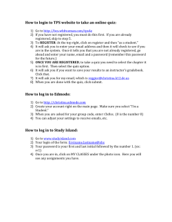


© Copyright 2026