1. health and fitness
2. disorders
3. mental disorder
4. depression

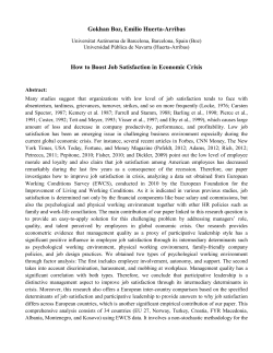
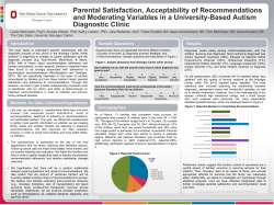
How much should we trust life satisfaction data?
Evidence from the Life in Transition Survey
Elena Nikolova and Peter Sanfey
Summary
We analyse responses to two similar life satisfaction questions asked during the same interview for each respondent
in a major cross-country household survey covering the transition region, Turkey and five western European
countries. We show that while the answers to the two questions are broadly consistent for most people, the
responses for some groups differ significantly. Older and less healthy respondents show systematically lower levels
of self-reported satisfaction in the later question, as do those living under less democratic, more repressive regimes.
We also find evidence that responses to the later question are influenced by preceding questions on socio-economic
status and social capital, and that response precision depends on the interviewee’s socio-economic status. Our
results have important implications for the design and length of household surveys that contain subjective questions.
Keywords: life satisfaction, measurement, Life in Transition Survey.
JEL Classification: D63, I31, P36.
Contact details: Elena Nikolova, One Exchange Square, London EC2A 2JN, United Kingdom
Phone: +44 20 7338 7931; Fax: +44 20 7338 6110; email: [email protected].
Elena Nikolova is Research Economist at the European Bank for Reconstruction and Development. Peter Sanfey is
Deputy Director of Country Strategy and Policy at the European Bank for Reconstruction and Development.
We are grateful to Ralph de Haas, Yannis Georgellis, Sergei Guriev, Milena Nikolova and seminar participants at the EBRD for helpful
comments and suggestions, and to Milena Djourelova and Simon Hess for excellent research assistance.
The working paper series has been produced to stimulate debate on the economic transformation of central and
eastern Europe and the CIS. Views presented are those of the authors and not necessarily of the EBRD.
Working Paper No.174
Prepared in January 2015
1
Introduction
In the past two decades, the study of life satisfaction, or “happiness”, has become a thriving area
of research in economics. There is now a firm body of evidence to support the view that surveys
of well-being can yield meaningful and policy-relevant information about people’s welfare. Increasingly, this research has spilled over into the policy arena, with institutions such as the OECD
routinely constructing cross-country measures of happiness and producing guidelines on the appropriate methodology.1 But what happens when people are asked twice in the same interview
about their well-being? Are the responses consistent or do they differ for some people, and if so,
how? These questions, which have received little attention in the literature so far, are the focus
of our paper.
Our analysis is based on the second round of the EBRD/World Bank Life in Transition Survey
(LiTS II), a nationally representative household-level survey. LiTS II was carried out in late
2010 across 29 transition countries of central and eastern Europe and the former Soviet Union,
Turkey and five western European countries (France, Germany, Italy, Sweden and the United
Kingdom). A unique feature of this survey is that respondents are asked about their overall
satisfaction with life at different points in the same interview, which allows us to study how
intervening questions change the interviewee’s initial life satisfaction answer. The first subjective
well-being question, which asks respondents to agree or disagree with the statement “All things
considered, I am satisfied with my life now” (on a five-point scale), appears relatively early in
the interview. In contrast, the second question, phrased as follows: “All things considered, how
satisfied or dissatisfied are you with your life as a whole these days? Please answer on a scale
of 1 to 10, where 1 means completely dissatisfied and 10 means completely satisfied”, is near
the end of the questionnaire. While the questions are quite similar, there are differences when it
comes to phrasing and scaling which may also drive the observed variation in responses.
Cojocaru and Diagne (2013) have looked at the consistency of the two measures and show that
the answers are highly correlated at the country level. Although our individual-level analysis
is broadly in line with such a conclusion, we also find that for approximately 14 per cent of
respondents the answers to the two life satisfaction questions differ significantly.2 In our analysis,
we test four specific hypotheses related to (1) the direction of the response switch (captured by
the actual response difference) and (2) the precision of the two responses (proxied by the absolute
value of the response difference).
• Responses to life satisfaction questions may be significantly affected by an individual’s
mood, which can change markedly during the interview. The LiTS questionnaire is lengthy,
with interviews typically lasting more than an hour. Therefore, an apparent drop in life
satisfaction between the first and second question could be related to age and health, as
older and less healthy people become tired and fed up as the interview progresses.
1 Life
satisfaction is a key component of the OECD’s “Better Life Initiative”, described in http://www.oecd.
org/statistics/measuring-well-being-and-progress.htm. The United Nations produces an annual report
on world happiness - see Helliwell et al. (2013).
2 We explain below what we mean by a “significant” difference between the two responses.
1
• The responses may be affected by context and framing effects. Some of the questions
and topics addressed between the first and second life satisfaction question may prompt
respondents to evaluate good or bad aspects of their lives. We explore the extent to which
answers to the second question appear to be influenced by socio-economic status, social
capital, views on issues such as trust and corruption, and events from the past.
• Differences in wording of the two questions may be important. Specifically, we test
whether in less democratic countries people who are invited to agree with a statement (the
format of the first subjective well-being question) may be more inclined to give positive
answers than when they are asked to score their response on a numerical scale (which is
what they are asked to do in the second question).
• In addition to leading to a downward bias in self-reported well-being in the second question, certain intervening questions and individual characteristics may affect the recall of
previous information and thus the measurement error in responses.
We find that several groups of people report a decrease in life satisfaction in the second question.
Those aged 63 and above and people who report themselves to be less healthy (on a 1-5 scale)
appear on average to experience a drop in life satisfaction during the interview. Higher education (both individual and parental), income and social capital have a positive effect on responses
to the second well-being question, though favourable opinions about institutions are either insignificant or, surprisingly, seem to bias life satisfaction scores downward in the second question.
Respondents in countries with notoriously weak democratic institutions, such as Tajikistan and
Uzbekistan, are more willing to “agree” that they are satisfied with life (in the first question) than
they are to give a corresponding high score on a 1-10 scale (in the second question). Lastly, our
results suggest that response precision is positively associated with individual socio-economic
status (captured by controls for education, income and employment status).
Since our regressions are based on cross-sectional data, a potential concern is that the results
may be driven by unobservable individual traits (Ferrer-i Carbonell and Frijters, 2004). We adopt
four complementary approaches to deal with such issues. First, by construction, our dependent
variable (the response difference to the two life satisfaction questions) eliminates individualspecific effects, which may otherwise have contaminated the estimates. Second, we control for a
rich set of observable individual characteristics, ranging from health and marital status to political
party membership. Third, we also include country dummies (in the baseline specification) as
well as dummies at the levels of sub-national administrative regions and even primary sampling
units (PSUs) (in the robustness checks). By comparing similar individuals within very narrow
geographical areas, our empirical analysis makes it less likely that the observed effects are driven
by fixed sub-national differences such as geography or culture. Finally, it is reassuring that
our results survive multiple robustness checks, such as the inclusion of interviewer fixed effects
or alternative estimation techniques. Although we cannot eliminate all sources of bias in our
cross-sectional data, our multi-pronged, micro-level approach makes us more confident that the
relationships which we uncover are likely to be causal.
We contribute to the literature in several ways. First, the unique research set-up implemented
in this paper provides us with the rare opportunity to identify the biases associated with data on
2
subjective well-being. More substantively, we complement a small but increasingly important literature which looks at how answers to life satisfaction questions vary with survey characteristics
ranging from order effects and the type of preceding questions to the accessibility and motivation
of respondents.3 While this work is largely based on surveys from single advanced countries,
we show that similar concerns about life satisfaction responses may be applicable in a broader
cross-section. In fact, the magnitude as well as source of biases which we uncover are remarkably similar when we compare the transition region with the six non-transition countries in our
sample (France, Germany, Italy, Sweden, Turkey, United Kingdom).4
Finally, our results have important implications for studies on the economics of happiness. The
finding that answers to two different questions on subjective well-being are broadly consistent for
most people is comforting as it suggests that such data are not unduly driven by random noise and
can in fact capture meaningful variation in life satisfaction. Similarly, our findings that reported
happiness changes little once respondents are asked a battery of sensitive political questions are
encouraging and stand in contrast to other work on the United States, such as Deaton (2012).
However, since life satisfaction responses are subject to non-trivial bias for respondents who are
older, less healthy and of lower socio-economic status, researchers should pay particular attention
to these groups when conducting econometric analyses. More generally, our results show that a
re-think may be needed regarding the design of future rounds of the LiTS (and possibly other
major household surveys that include questions on subjective well-being), which we discuss in
more detail in the conclusion.
3 We
review these contributions in more detail in the following section.
a comparison involves the caveat that the transition sample is much bigger than the non-transition one.
4 Such
3
2
Previous literature
While economists have paid increasing attention to studying the determinants of life satisfaction,
the literature examining issues of measurement has been slower to develop.5 To the best of our
knowledge, there are no prior studies seeking to examine how reported life satisfaction may vary
within the same interview in a large cross-country survey such as the LiTS.
At the same time, we build on several influential contributions seeking to understand the possible biases involved in subjective well-being responses.6 Comparing daily data from the Gallup
World Poll in the United States, Deaton (2012) finds that life satisfaction measures are extremely
dependent on question ordering. He exploits the fact that in early 2009, Gallup randomly split the
sample of respondents, with half of interviewees being asked questions on political preferences
prior to the life satisfaction question, while for the other half of respondents the life satisfaction
question came first. It turns out that the former set-up reduces substantially self-reported wellbeing, and that the magnitude of this reduction is in fact much higher than the perceived impact
of the Great Recession.7 In contrast, using an approach that is perhaps closest to ours, Krueger
and Schkade (2008) find that two different measures of life satisfaction (a standard survey question and data on affective experience collected using the Day Reconstruction Method two weeks
after the interview) have a reasonably high serial correlation (0.6) for a sample of 229 women in
the United States. Although this Chart is lower than the reliability ratios for objective measures
such as education or income, the authors suggest that it is probably sufficient to yield informative
measures in large samples.8
Life satisfaction data may be subject to additional biases. Conti and Pudney (2011) show that
a seemingly minor change in the job satisfaction question in the British Household Panel Survey (BHPS) – the switch from partial use of textual labels (in addition to numerical labels) as
anchors for the response scale (in the 1991 survey) to their full use (in the 1992 survey) – leads
to large inconsistencies in the distribution of responses. In particular, women are more likely
to pick responses accompanied by textual labels. The authors find that survey mode administration (face-to-face or self-administered) and context (presence of partner and children) also
matter, more so for women than for men.9 Interviewer characteristics (including gender and in5 See
Frey and Stutzer (2010), Layard (2005) and Powdthavee (2010) for useful surveys of the literature on the
economics of happiness. There is also a small but growing literature on life satisfaction in the transition region (which
comprises the majority of our sample), some of which has tried to explain the relatively low levels of happiness
compared with other parts of the world (see Sanfey and Teksoz (2007), Guriev and Zhuravskaya (2009), Kornai
(2006), Senik (2009) and Dabalen and Paul (2011)).
6 See Kahneman and Krueger (2006) for an earlier survey of this literature.
7 In the psychology literature, it has long been recognised that self-reported answers on attitudes and feelings
can be affected by context and ordering of questions. See, for example, Schwarz (1999) and Schimmack and Oishi
(2005).
8 See also Studer (2012) who utilises a randomised design in a Dutch internet panel survey to argue that a continuous life satisfaction scale provides more discriminating power than a discrete one.
9 Dolan and Kavetsos (2012) find that in the 2011 Annual Population Survey in the United Kingdom, respondents
who are interviewed over the phone are consistently happier than those in face-to-face interviews, and that the
determinants of subjective well-being depend on survey mode. Using multiple waves of the Eurobarometer data,
Kavetsos et al. (2014) find that life satisfaction depends on the day and month of the interview (but not time of day),
and that subjective well-being is significantly reduced when others are present.
4
terviewing experience) may also sway life satisfaction responses (Chadi, 2013; Kassenboehmer
and Haisken-DeNew, 2012).
Yet another strand of the literature examines to what extent subjective well-being responses vary
with interviewees’ accessibility and motivation. Using the reported number of call attempts in
the University of Michigan’s Survey of Consumers, Heffetz and Rabin (2013) show that lifesatisfaction levels are higher among easy-to-reach women (compared with easy-to-reach men),
but that hard-to-reach men are happier than hard-to-reach women. The authors warn that these
unexpected effects of sample selection are likely to be even more severe when fewer contact
attempts are made. In a similar vein, Chadi (2014) shows that in the German Socio-Economic
Panel Study, respondents with a higher number of interviewer contacts report lower levels of
life satisfaction, possibly because such respondents are less motivated to go through with the
interview.10
10 If
a selected respondent was unavailable, LiTS enumerators conducted up to three follow-up visits, though
unfortunately an exact breakdown for each respondent is not available in our data.
5
3
Data description
Our analysis is based on the second round of the Life in Transition Survey, which covers virtually
all transition countries in central and eastern Europe and the former Soviet Union (as well as
Mongolia and Turkey), except Turkmenistan.11 Unlike the first round of the survey, LiTS II also
includes five western European “comparator” countries. All of these countries are included in
the analysis below, although as we discuss in the robustness section, results are very similar if we
only restrict our sample to countries in the transition region.
Respondents were drawn randomly, using a two-stage sampling method with primary and secondary sampling units. The Primary Sampling Units (PSU) are electoral districts, polling station
territories, census enumeration districts or geo-administrative divisions, while Secondary Sampling Units are households. Each country has a minimum of 50 PSUs with each PSU containing
around 20 households (for a total of approximately 1,000 observations), with the exception of
Poland, Russia, Serbia, Ukraine and Uzbekistan, where 75 PSUs containing around 20 households each were drawn (for a total of approximately 1,500 observations). The head of the household or another knowledgeable household member answered the Household Roster and questions
about housing and expenses, while all other modules – including the two different life satisfaction
question – were answered by a randomly drawn adult (over 18 years of age) from the household
in a face-to-face interview with no substitutions possible.12
In Section 3, interviewees are asked a series of questions about attitudes and values. The section opens with the respondent being asked: “To what extent do you agree with the following
statements?” One of the statements is:“All things considered, I am satisfied with my life now.”
The response could be one of the following: strongly disagree, disagree, neither disagree nor
agree, agree, and strongly agree.13 The answers can be converted to a numerical 1-5 scale, where
1 represents “strongly disagree” and 5 “strongly agree.” Section 7 is entitled “Miscellaneous
questions” and covers various aspects of the interviewee’s background and activities. The final
question in this section is: “All things considered, how satisfied or dissatisfied are you with your
life as a whole these days? Please answer on a scale of 1 to 10, where 1 means completely dissatisfied and 10 means completely satisfied.” Showcards were used to present the answer options to
the respondent for both questions. The LiTS records information on the duration, date and time
of the interview, but inconsistent enforcement means that these data are less reliable (in some
cases, our sample also drops significantly). We also obtained information on the identity of the
interviewer (captured by an interviewer dummy variable) for all countries except Italy. The results from specifications which control for interview duration and interviewer identity (presented
in the online Appendix) are consistent with our baseline findings below.
Charts 1 and 2 show how the scores in these two questions are distributed. The modal response
to the first question is “agree” (score of 4), and the simple average of all responses is 3.18. The
11 Further
details on the Life in Transition Survey, and the full data set, can be accessed at http://www.ebrd.
com/pages/research/economics/data/lits.shtml.
12 The other modules are: Attitudes and Values; Climate Change; Labour, Education and Entrepreneurial Activity;
Governance, Miscellaneous Questions, and Impact of the Crisis (the latter also answered by the household head).
13 “Do not know” and “not applicable” are also allowed, but these answers are disregarded in this paper.
6
modal response to the second question is just 5 (on the 1 to 10 scale) with a simple average of
5.52.
0
10
Per cent
20
30
40
Chart 1: Distribution of responses – first life satisfaction question
0
1
2
3
4
All things considered,I am satisfied with my life now
5
0
5
Per cent
10
15
20
25
Chart 2: Distribution of responses – second life satisfaction question
1
2
3
4
5
6
7
8
9
10
All things considered, how satisfied or dissatisfied are you with your life as a whole these days?
7
To explore this further, we look at how the responses differ at the individual level. We construct
a nine-point index, D1 as follows: define the first satisfaction question as Q1 and the second one
as Q2 . Then:
D1 = S2 − S1 ,
(1)
where S2 = 1 if the answer to Q2 = 1 or 2, S2 = 2 if the answer is 3 or 4,..., S2 = 5 if the answer =
9 or 10, and S1 = [1,...,5], as described above. D1 is therefore on a 9-point scale, ranging from -4
to 4. That is, someone who “strongly agrees” that, all things considered, he/she is satisfied with
life now but scores the second question at 1 or 2 would have a D1 score of -4, whereas “strongly
disagree” on the first question, combined with 9 or 10 on the second question would be a D1
score of 4. Chart 3 shows the distribution of D1 across the entire sample. Not surprisingly, the
modal score is 0 (with a mean of -0.15 and a standard deviation of 1.07), suggesting a relatively
high degree of comparability across the two measures of life satisfaction, consistent with the
findings of Cojocaru and Diagne (2013). However, 14.39 per cent of the sample show a significant
deviation in their answers, as captured by scores of 2 and above or -2 and below. The next
section tries to explain the variation across individuals by testing econometrically the hypotheses
mentioned in the introduction.
0
10
Per cent
20
30
40
Chart 3: Histogram of the nine-point difference in responses
-4
-3
-2
-1
0
1
Nine-point difference
8
2
3
4
4
Econometric analysis
We estimate the following equation:
D1ik = αik + β1 AgeDummiesik + β2 Healthik + β3 MaritalStatusik + Xik β4 + γk + εik ,
(2)
where for each individual i in country k Age Dummiesik is a set of age dummies (with the cohort
aged 42-52 the omitted category), Healthik is the respondent’s self-assessed health on a scale of
1 (very bad) to 5 (very good), and Marital Statusik is a dummy variable taking the value of 1
if the respondent is married and 0 otherwise. Xik is a matrix of additional controls which vary
across specifications and include the following broad categories: (1) individual socio-economic
characteristics (level of education, income and whether the individual was employed in the past
12 months); (2) parental background (father’s education and whether the respondent or his parents/grandparents were injured, killed or displaced during the second world war); (3) perceptions
of institutions (opinion about corruption, trust in institutions, the degree to which the respondent
believes effective institutions exist in the country, and support for income equality); and (4) social capital (how often the respondent meets up with friends, whether he/she is a member of a
political party, and whether he/she is an active member of various social organisations). γk is a
country fixed effect, and standard errors are clustered at the country level. Survey weights, which
ensure that the data are representative at the country level, are used in all specifications. More
information on the variables is available in the online Appendix.
We include age and health on the grounds that older and less healthy people may find their mood,
and hence their feeling of life satisfaction, dropping during the lengthy interview. Therefore, we
test if β1 < 0 (for individuals in the highest age categories) and β2 > 0. In the happiness literature
marital status is usually associated with higher levels of life satisfaction, and inclusion of this
variable shortly before the second life satisfaction question may temporarily raise the mood of
those who are married (implying that β3 > 0). Similarly, the literature shows that life satisfaction
is positively correlated with income, education and employment. Being reminded of one’s status
on these matters before the second life satisfaction question may give a boost to the index for
those who score well on these counts, and conversely may temporarily depress those who are
uneducated, with low income or unemployed. Respondents with a more favourable parental
background, better perceptions of institutions, and more social capital should also be more likely
to report higher levels of life satisfaction in the second question as they are reminded about these
aspects of their lives, so we expect that β4 > 0. Country dummies, in addition to capturing fixed
characteristics like geography or historical factors, may also allow us to understand if respondents
in more repressive, less democratic regimes are inclined to overstate life satisfaction when invited
to agree with the interviewer (on the grounds that people in these countries may be reluctant to
“disagree” with the questioner in an official interview).14
Since our data set is not an individual panel, an important issue relates to the bias associated with
unobservable characteristics, either at the individual, country or locality level. We believe that
such a critique is less convincing in our case for several reasons. First, since we calculate our
14 Even
though LiTS respondents are guaranteed anonymity, some may still be nervous about giving honest re-
sponses.
9
dependent variable using the response difference between the second and first life satisfaction
question, fixed individual characteristics disappear. Moreover, we show that our estimates are
robust to including a wide range of observable characteristics, such as age and marital status,
social capital and interviewer characteristics. Crucially, our specifications include either country
dummies (in the baseline specification) or dummies at the levels of sub-national administrative
regions and even primary sampling units (PSUs) (in the robustness checks). We thus compare
similar individuals within narrow geographical units (such as villages or city neighbourhoods
when we look at within-PSU variation), which makes it less likely that our results are driven by
spurious correlations.
Table 1 empirically tests the first three hypotheses on which we elaborated in the introduction.
Column (1) shows that being in the highest age group (aged 63 and above) has a negative and
statistically significant impact on the difference index, consistent with the notion that subjective well-being dips during the interview among the elderly. On average, older respondents report levels of happiness in the second life satisfaction question which are around 0.09 points
lower, though this magnitude drops slightly when we introduce additional covariates in the other
columns. While such an effect may appear small, one must keep in mind that the dependent variable is distributed with a very small mean (-0.15) but a relatively large standard deviation (1.07).
Similarly, health status is also significantly and positively correlated with the difference index.
However, the coefficient on being married, while positive, is imprecisely estimated.
The (unreported) coefficients of the country dummies are all significantly positive relative to the
reference country, Russia, with the exception of the following countries: Azerbaijan, Belarus,
Bulgaria, Georgia, Kazakhstan, Kyrgyz Republic, Kosovo, Tajikistan, Turkey and Uzbekistan.15
With the exception of Bulgaria, these countries have had a chequered democratic experience
since transition began, as captured by cross-country measures of democratic institutions, such
as the Polity score.16 These results are consistent with our hypothesis that respondents in less
democratic countries may be more likely to agree with the first life satisfaction question and
revise their response downward in the later question.
In the remaining columns of Table 1, we present the results of several specifications with framing
variables, where different groups of variables are added separately to the baseline model of column 1. In column 2, we add the respondent’s level of education (on a scale of 1 to 6, with 1 being
no education and 6 being Master’s and Ph.D.-level education), income (as measured by selfassessment of one’s position on a 10-step income ladder) and a dummy variable for employment
in the past 12 months. Both education and income are positive and statistically significant, pointing to possible framing effects of questions about socio-economic status. A one-unit increase in
education (for instance, from no education to primary education, or from Bachelor-level education to Master’s/Ph.D) makes a respondent nearly 0.03 points happier in the second question, with
a slightly higher effect of a one-standard deviation rise in income (0.042 points). These findings
seem to outweigh a possible countervailing effect whereby richer and more educated people have
a higher opportunity cost of time and hence may become impatient and dissatisfied by the time
of the second life satisfaction question.
15 Estimates
lose significance for Uzbekistan, Kazakhstan, Georgia and Turkey when all covariates are included in
column 6, and the estimate for Belarus turns positive.
16 See http://www.systemicpeace.org/ for more information on the Polity data.
10
Column 3 instead adds to the baseline specification two variables that relate (largely) to the
respondent’s parents and grandparents. One is the level of the father’s education (measured in
years of full-time education), which has a positive impact on the difference index, and suggests
that those whose fathers have on average four more years of education (roughly the difference
between high-school and university) report happiness scores in the second question that are nearly
0.06 points higher. The other variable is a dummy for whether the respondent, or any of his/her
parents or grandparents, were killed, injured or forced to move during the second world war.
Because the latter question is asked just before the second life satisfaction question, one might
expect an impact on responses. It turns out that there is either no impact, or even a positive one
(when only displacement is considered in unreported results). While this may be surprising, it
has been noted in the psychology literature that the recall of negative events in the distant past (as
opposed to more recent ones) can result in higher life satisfaction than for those recalling positive
events.17
In column 4 we add several variables relating to attitudes and beliefs about trust, corruption and
the effectiveness of institutions. Although our expectation was that a negative view on these
issues – for example, a belief that corruption is widespread – would be associated with a drop in
the difference index, the results are either insignificant or go the opposite way. This is a puzzle
that merits further investigation, but one possibility could be that more trustworthy people may be
more likely to agree with the first life satisfaction question and reverse their response afterward.
Interestingly, however, there is a statistically significant and negative relationship between the
dummy variable capturing whether the respondent supports income equality and the difference
in life satisfaction, in the magnitude of around 0.07 points.
In column 5 we introduce several social capital variables: whether the person meets regularly
with friends (on a scale of 1 (never) to 5 (most days)), and participates in a political party (a
dummy variable) or different organisations (ranging from 0 to 9 to capture all the organisations
in which the respondent may be involved). In this case, we find supportive evidence for framing
effects for two out of the three variables. Those who say they rarely or never meet up with friends
tend to record lower life satisfaction scores in the second question, while those who are active in
various organisations record a boost to their numerical life satisfaction. Membership in a political
party is not significant. It is also possible that respondents with social capital find the interview
more enjoyable, prompting them to give a higher answer to the second life satisfaction question.
Lastly, column 6 reports the results of an all-encompassing equation, including simultaneously
all variables from the previous columns. The main conclusions for income, education, father’s
education and the social capital variables, as well as the country dummies, remain broadly valid,
but some other results, including those relating to health and age, lose statistical significance,
possibly because of including multiple controls in the same regression.
To test to what extent intervening questions and individual characteristics affect the recall of
information and measurement error in life satisfaction responses, we next run a version of our
estimating equation in which we simply take the absolute value of the difference as a dependent
variable, thus ignoring whether answers to the second satisfaction question are higher or lower
17 See
Schwarz (1999).
11
than the first one (see Chart A1 in the online Appendix for a snapshot of the distribution of this
variable). The results, which are presented in Table 2, show that individuals with lower socioeconomic status (captured by education, income and employment dummy) are less likely to give
consistent responses. Using the point estimates in column 2, being employed increases response
precision by around 0.03 points (3.8 per cent relative to the mean of the dependent variable), while
the effect of a one-step increase in perceived income (on a ten-step income ladder) is around 0.02
points (2.4 per cent relative to the mean of the dependent variable).18 This suggests that data
on well-being for uneducated, low-income or unemployed groups may be subject to more noise,
implying the need for robustness checks on these groups in life satisfaction studies. Controls
for father’s education, perceptions of institutions and social capital are not significant and do not
change these results, hence they are omitted from the table to conserve space.
Table 1: Determinants of difference in answers to the two life satisfaction questions
(1)
Nine-point difference
(2)
Nine-point difference
(3)
Nine-point difference
Baseline
Health
0.0379∗∗∗
(0.0111)
0.0224∗
(0.0117)
0.0231∗
(0.0122)
Married
0.0162
(0.0144)
0.00764
(0.0144)
0.0109
(0.0163)
Age 18-22
0.0163
(0.0326)
0.0191
(0.0337)
0.00859
(0.0385)
Age 23-32
−0.00759
(0.0225)
−0.0171
(0.0237)
−0.0441
(0.0265)
Age 33-42
0.00501
(0.0158)
0.00836
(0.0161)
−0.00558
(0.0188)
Age 53-62
0.00141
(0.0196)
0.00859
(0.0201)
0.0167
(0.0253)
−0.0937∗∗∗
(0.0213)
−0.0657∗∗∗
(0.0214)
−0.0584∗∗
(0.0258)
Age 63+
Individual SES
Education
0.0253∗∗∗
(0.00609)
Income
0.0254∗∗∗
(0.00771)
Employed
0.00670
(0.0196)
Parental background
Father’s education
0.0141∗∗∗
(0.00263)
Affected by war
0.0128
(0.0204)
Country dummies
Observations
R2
X
X
37792
0.0428
36259
0.0465
X
26045
0.0481
Notes: Dependent variable is the nine-point difference between the second life satisfaction question and the first life satisfaction question. OLS - Coefficients are reported. Standard errors are
clustered at the country level. Significance levels: * p < 0.1, ** p < 0.05, *** p < 0.01.
18 The
absolute difference has a mean of 0.77 with a standard deviation of 0.76.
12
Table 1 (continued)
(4)
Nine-point difference
(5)
Nine-point difference
(6)
Nine-point difference
Baseline
Health
0.0515∗∗∗
(0.00961)
0.0359∗∗∗
(0.0108)
0.0204
(0.0124)
Married
0.0289∗∗
(0.0133)
0.0167
(0.0147)
0.00897
(0.0166)
Age 18-22
0.0240
(0.0315)
0.00679
(0.0320)
−0.00325
(0.0461)
Age 23-32
−0.0126
(0.0224)
−0.0121
(0.0221)
−0.0396
(0.0257)
Age 33-42
0.00282
(0.0177)
0.00542
(0.0157)
−0.00145
(0.0183)
Age 53-62
−0.00403
(0.0226)
−0.000264
(0.0194)
0.0203
(0.0289)
Age 63+
−0.0620∗∗
(0.0263)
−0.0916∗∗∗
(0.0218)
−0.00349
(0.0269)
Individual SES
Education
0.0111∗
(0.00627)
Income
0.0306∗∗∗
(0.00846)
Employed
0.00776
(0.0228)
Parental background
Father’s education
0.00911∗∗∗
(0.00277)
Affected by war
0.0271
(0.0226)
Perception of institutions
Trust institutions
−0.0756∗∗∗
(0.0153)
−0.0889∗∗∗
(0.0181)
Effective institutions exist
−0.102∗∗∗
(0.0179)
−0.0949∗∗∗
(0.0211)
Political liberties exist
0.00966
(0.0200)
0.0112
(0.0227)
Corruption exists
0.00136
(0.00196)
0.00138
(0.00199)
−0.0662∗∗∗
(0.0194)
−0.0610∗∗∗
(0.0209)
Incomes should be more equal
Social capital
0.0174∗∗
(0.00766)
Meet up with friends
−0.0502
(0.0332)
Member of a political party
Active member of organisations
Country dummies
Observations
R2
X
26945
0.0567
0.0260∗∗
(0.0103)
−0.0691
(0.0432)
0.0256∗∗∗
(0.00932)
0.0184
(0.0111)
X
X
37124
0.0435
18939
0.0670
Notes: Dependent variable is the nine-point difference between the second life satisfaction question and the
first life satisfaction question. OLS - Coefficients are reported. Standard errors are clustered at the country
level. Significance levels: * p < 0.1, ** p < 0.05, *** p < 0.01.
13
Table 2: Determinants of absolute difference in answers to the two life satisfaction questions
(1)
Absolute difference
(2)
Absolute difference
Baseline
Health
−0.00678
(0.00732)
−0.0104
(0.00987)
Married
0.00147
(0.0110)
0.00247
(0.0162)
Age 18-22
−0.0195
(0.0137)
−0.0470∗∗
(0.0217)
Age 23-32
−0.00517
(0.0110)
−0.00817
(0.0185)
Age 33-42
−0.0167
(0.0108)
−0.0132
(0.0142)
Age 53-62
−0.0230∗
(0.0127)
−0.0275
(0.0172)
Age 63+
−0.0222
(0.0154)
−0.0297
(0.0204)
Education
−0.00918∗∗
(0.00340)
−0.0100∗∗
(0.00474)
Income
−0.0197∗∗∗
(0.00519)
−0.0183∗∗∗
(0.00594)
Employed
−0.0335∗∗∗
(0.0100)
−0.0293∗
(0.0155)
Individual SES
Parental background
X
Perception of institutions
X
Social capital
X
Country dummies
Observations
R2
X
36259
0.0318
X
18939
0.0385
Notes: Dependent variable is the absolute difference between the second
life satisfaction question and the first life satisfaction question. OLS Coefficients are reported. Standard errors are clustered at the country
level. Significance levels: * p < 0.1, ** p < 0.05, *** p < 0.01.
To assess the salience of the life satisfaction response differences which we have analysed, we
estimate two separate life satisfaction regressions (in levels) similar to those used in the happiness
literature in Table A1. In column 1, we use the first question as a dependent variable, while
in column 2 we run exactly the same specification using the second life satisfaction question
(for comparability, both questions are coded on a 1-5 scale).19 Columns 3 and 4 test for the
equality of each pair of coefficients and show that we can reject equivalence for 5 out of the 10
independent variables. When life satisfaction is proxied with the second question, education,
income and father’s education exhibit a stronger effect (with the latter coefficient turning from
insignificant in column 1 to significant in column 2). The higher coefficient on age and the
lower coefficient on age squared in column 2 suggest that the U-shaped effect is flatter when
the dependent variable is obtained from answers to the second life satisfaction question (both
regressions show that happiness reaches its nadir when respondents are around 42 years old).
In other words, while the correlates of the two well-being questions appear broadly similar in
19 Including
the number of children in the household (in unreported specifications) does not change these results.
14
our data, there are nevertheless several disparities which researchers should take into account. In
addition, the magnitude and sign of the coefficients in Table A1 are very similar to those obtained
in other cross-country work (using the World Values Survey) covering both transition and nontransition countries (Guriev and Zhuravskaya, 2009; Sanfey and Teksoz, 2007), which indicates
that the results in this paper are not driven by the idiosyncrasies of the LiTS.
15
5
Extensions and robustness
Are the life satisfaction biases which we uncover different across transition and non-transition
countries? Keeping in mind the caveat that our sample contains only six non-transition countries
(France, Germany, Italy, Sweden, Turkey and the United Kingdom), in Table A2 we present results from interacting our independent variables with a transition country dummy (only variables
with significant interaction terms are reported to conserve space). We find that in transition countries those who are healthier, married and more trusting of institutions are more likely to report a
lower life satisfaction score in the second question, while those who are richer are more likely to
overreport happiness in the second question. None of the transition dummy interactions with the
other independent variables are significant, suggesting that response inconsistencies are similar
across transition and non-transition countries.
We test the robustness of our results in Table 3. In each case, we take the inclusive version of
the model; that is, the equivalent of column 6 in Table 1. To further alleviate concerns about
local-level unobservable characteristics, column 1 replaces the country dummies with dummies
at the level of sub-national administrative regions. Instead, column 2 includes dummies at the
primary sampling unit level (PSU), which essentially implies that we are comparing individuals
within very small geographic units such as villages or city neighbourhoods (both specifications
cluster the errors at either the regional or PSU level). Finally, column 3 introduces interviewer
dummies.20 In all three cases, the results are broadly consistent with those in Table 1, although
sometimes in columns 2 and 3 they are less precisely estimated, possibly because we are dropping
useful variation from our estimations.21
We implement several additional robustness tests in the online Appendix. In Tables A3 and
A4 we relax the cardinality assumption on which our OLS regressions are based and show that
our results are robust to using ordinal models (multinomial logit and ordered probit; marginal
coefficients are reported in both tables). Following Conti and Pudney (2011), in Table A3 we
distinguish three states: S2 > S1 , S2 < S1 and S2 = S1 (the latter being the reference category). To
conserve space in Table A4, we only report the coefficient estimates for the difference categories
-2, 0 and 2. Results are broadly in line with our baseline specification: respondents with low
socioeconomic status are more likely to under-report happiness in the second question, while
those with social capital are less likely to record a lower life satisfaction score in the second
question. The results on institutional perceptions and income equality also survive.
In Table A5, we control for interview day and time and interview duration. Although results are
largely consistent, estimates should be treated with caution since data limitations shrink our sample considerably.22 In unreported specifications, we failed to find an interaction effect between
20 Interviewer
information is not available for Italy.
income and the extent to which the respondent meets up with friends lose significance in column 2, we
also ran specifications in which we include the average value of these variables for all respondents in the individual’s
PSU (excluding the respondent himself/herself). Our results indicate that this specification explains around 46 per
cent of the observed variation in individual income and around 39 per cent of the observed variation in the individual
propensity to meet up with friends, likely because these variables are highly correlated at the local level.
22 Although interview duration may be endogenous to various individual characteristics, we do not find that any
of our independent variables explain it in our sample.
21 Since
16
interview duration and any of our independent variables, though of course this could arise from
attenuation bias due to measurement error in the duration variable.
We probe the sensitivity of our results to an alternative and more flexible coding scheme of
our dependent variable (which now ranges from -2 to 2) in Table A6. More precisely, if the
respondent gave an answer of 1 or 2 in the first question, we regarded any answer of 1, 2, 3, or
4 in the second question as consistent and coded these cases as having a difference score of 0.
For respondents who picked either 1 or 2 in the first question but 5 or 6 in the second question,
we coded a difference score of 1. If a respondent picked 1 or 2 in the first question but 7, 8, 9 or
10 in the second question, then the difference score takes a value of 2. Following a similar logic,
respondents with a life satisfaction score in the first question of 4 or 5 can pick 7, 8, 9 or 10 in the
second question (for a difference score of 0), 5 or 6 (for a difference score of -1) and 1, 2, 3 or 4
(for a difference score of -2). Respondents who picked the middle category in the first question
(3) can choose either 5 or 6 in the second question (for a difference score of 0), 1, 2, 3 or 4 (for a
difference score of -1), or 7, 8, 9 or 10 (for a difference score of 1). The results in Table A6 are
very similar to those we presented earlier.
In unreported specifications, we recoded our dependent variable as a standardised difference; that
is, converting S1 and S2 to standardised scores (subtracting the mean across all observations and
dividing by the standard deviation) and taking the difference. In a different specification, we
dropped difference scores of -4 and 4. In both variants, the main conclusions derived from the
model estimated earlier still hold.
17
Table 3: Robustness table
(1)
Nine-point difference
(2)
Nine-point difference
(3)
Nine-point difference
Baseline
Health
0.0250∗
(0.0137)
0.0200
(0.0126)
0.0198
(0.0126)
Married
0.00501
(0.0179)
0.0247
(0.0186)
0.0277
(0.0198)
Age 18-22
−0.0126
(0.0417)
−0.00778
(0.0413)
0.0152
(0.0423)
Age 23-32
−0.0440∗
(0.0236)
−0.0264
(0.0270)
−0.0235
(0.0307)
Age 33-42
−0.00109
(0.0219)
0.0106
(0.0251)
0.0115
(0.0279)
Age 53-62
0.0154
(0.0288)
0.00437
(0.0280)
0.00827
(0.0293)
Age 63+
0.00559
(0.0385)
−0.00308
(0.0315)
−0.0379
(0.0318)
Individual SES
Education
0.0136∗
(0.00749)
0.0168∗∗
(0.00767)
0.00975
(0.00811)
Income
0.0243∗∗∗
(0.00687)
0.0101
(0.00732)
0.0131∗
(0.00756)
Employed
0.0188
(0.0190)
0.00749
(0.0213)
Father’s education
0.00823∗∗∗
(0.00292)
0.00882∗∗∗
(0.00260)
0.00977∗∗∗
(0.00273)
Affected by war
0.0157
(0.0197)
0.0109
(0.0209)
0.0167
(0.0220)
Trust institutions
−0.0879∗∗∗
(0.0154)
−0.0839∗∗∗
(0.0165)
−0.0743∗∗∗
(0.0177)
Effective institutions exist
−0.0787∗∗∗
(0.0273)
−0.0645∗∗∗
(0.0189)
−0.0823∗∗∗
(0.0189)
0.0449∗∗
(0.0200)
0.0372∗
(0.0222)
0.0158
(0.0223)
Corruption exists
−0.000257
(0.00181)
−0.000180
(0.00224)
−0.000853
(0.00244)
Incomes should be more equal
−0.0591∗∗∗
(0.0204)
−0.0470∗∗
(0.0218)
−0.0442∗∗
(0.0224)
0.0164∗
(0.00957)
0.0101
(0.0110)
0.00221
(0.0109)
−0.0691∗
(0.0382)
−0.0311
(0.0377)
0.0290∗
(0.0150)
0.0147
(0.0136)
−0.0200
(0.0213)
Parental background
Perception of institutions
Political liberties exist
Social capital
Meet up with friends
Member of a political party
−0.0706
(0.0484)
Active member of organisations
0.0318∗∗
(0.0129)
Region dummies
X
X
PSU dummies
X
Interviewer dummies
Observations
R2
18939
0.131
18939
0.260
18176
0.296
Notes: OLS - Coefficients are reported. Standard errors are clustered at the country level. Significance
levels: * p < 0.1, ** p < 0.05, *** p < 0.01.
18
6
Conclusion
We exploit the rare opportunity to observe answers to two similar life satisfaction questions asked
during the same interview in the LiTS. We conclude that the ordering and wording of questions on
subjective well-being can influence the responses, and that this fact should be taken into account
when designing household questionnaires and interpreting the resulting data. To summarise: we
found that there is a high degree of consistency between the answers to the two questions on
life satisfaction. That is good news for the happiness literature, because it helps to rebut the
view that data on subjective well-being are noisy and unduly influenced by whims. Furthermore,
our findings that sensitive questions on institutions and corruption do not bias responses in the
second life satisfaction question downward is encouraging, particularly in light of the opposite
conclusion reached by Deaton (2012) for the United States.
However, our analysis also shows that for around 14 per cent of respondents, life satisfaction
changed significantly from the first to the second question. Older and less healthy people appear
to experience a drop in satisfaction during the interview, and intervening questions related to individual SES, parental background and social capital can trigger changes in well-being, perhaps
by reminding people of pleasant or unpleasant aspects of their lives. The striking differences in
responses to the two questions in more repressive regimes indicates the need for care in interpreting other questions where the interviewee is invited to agree or disagree with the interviewer.
We also find that the life satisfaction responses of those who have less income, education or are
unemployed are more noisy.
These results point to a number of methodological suggestions for future research in this area.
First, the length of the questionnaire needs to be considered and, if possible, shortened. The fact
that older and relatively unhealthy people show a drop in life satisfaction during the interview
suggests that their responses to other questions that come towards the end may be contaminated
by fatigue. In addition, researchers studying the determinants of life satisfaction may wish to
run robustness tests on those sub-samples of respondents which we identified as more prone to
“imprecise” answers. More broadly, the “gold-standard” approach would be to use two identical
life satisfaction questions whose position is randomly assigned in the survey. Unfortunately, a
research design of this type may be difficult and expensive to carry out in a large cross-country
survey such as the LiTS. In the absence of such an approach, we believe that the research strategy
adopted in this paper provides an important methodological contribution.
19
References
A. Chadi (2013), “The role of interviewer encounters in panel responses on life satisfaction”,
Economics Letters, 121(3), 550–554.
A. Chadi (2014), “Dissatisfied with life or with being interviewed? Happiness and motivation to
participate in a survey”, SOEP Working paper 639, (639).
A. Cojocaru and M. F. Diagne (2013), “How reliable and consistent are subjective measures of
welfare in Europe and Central Asia? Evidence from the second Life in Transition Survey”,
World Bank Policy Research Working Paper 6359, (6359).
G. Conti and S. Pudney (2011), “Survey design and the analysis of satisfaction”, Review of Economics and Statistics, 93(3), 1087–1093.
A. Dabalen and S. Paul (2011), “History of events and life-satisfaction in transition countries”,
World Bank Policy Research Working Paper 5526, (5526).
A. Deaton (2012), “The financial crisis and the well-being of Americans 2011 OEP Hicks Lecture”, Oxford economic papers, 64(1), 1–26.
P. Dolan and G. Kavetsos (2012), “Happy talk: mode of administration effects on subjective
well-being”, CEP Discussion Paper 1159, (1159).
A. Ferrer-i Carbonell and P. Frijters (2004), “How important is methodology for the estimates of
the determinants of happiness?”, The Economic Journal, 114(497), 641–659.
B. S. Frey and A. Stutzer (2010), Happiness and economics: how the economy and institutions
affect human well-being, Princeton University Press.
S. Guriev and E. Zhuravskaya (2009), “Unhappiness in transition”, Journal of Economic Perspectives, 23(2), 143–68.
O. Heffetz and M. Rabin (2013), “Conclusions regarding cross-group differences in happiness
depend on difficulty of reaching respondents”, The American Economic Review, 103(7), 3001–
3021.
J. F. Helliwell, R. Layard, J. Sachs, and E. C. Council (2013), World happiness report 2013,
Sustainable Development Solutions Network.
D. Kahneman and A. B. Krueger (2006), “Developments in the measurement of subjective wellbeing”, The Journal of Economic Perspectives, 20(1), 3–24.
S. C. Kassenboehmer and J. P. Haisken-DeNew (2012), “Heresy or enlightenment? The wellbeing age U-shape effect is flat”, Economics Letters, 117(1), 235–238.
G. Kavetsos, M. Dimitriadou, and P. Dolan (2014), “Measuring happiness: context matters”,
Applied Economics Letters, 21(5), 308–311.
J. Kornai (2006), “The great transformation of central eastern Europe”, Economics of Transition,
14(2), 207–244.
20
A. B. Krueger and D. A. Schkade (2008), “The reliability of subjective well-being measures”,
Journal of Public Economics, 92(8), 1833–1845.
R. Layard (2005), “Happiness: lessons from a new science”, London: Allen Lane.
N. Powdthavee (2010), The happiness equation: the surprising economics of our most valuable
asset, Icon Books.
P. Sanfey and U. Teksoz (2007), “Does transition make you happy?”, Economics of Transition,
15(4), 707–731.
U. Schimmack and S. Oishi (2005), “The influence of chronically and temporarily accessible
information on life satisfaction judgments”, Journal of Personality and Social Psychology,
89(3), 395.
N. Schwarz (1999), “Self-reports: how the questions shape the answers”, American Psychologist,
54(2), 93.
C. Senik (2009), “Direct evidence on income comparisons and their welfare effects”, Journal of
Economic Behavior & Organization, 72(1), 408–424.
R. Studer (2012), “Does it matter how happiness is measured? Evidence from a randomized
controlled experiment”, Journal of Economic and Social Measurement, 37(4), 317–336.
21
ONLINE APPENDIX
Additional charts and tables
0
10
Per cent
20
30
40
50
Chart A1: Histogram of the absolute difference in responses
-1
0
1
2
Absolute difference
22
3
4
Table A1: Life satisfaction regressions using S1 and S2
(1)
S1
(2)
S2
(3)
χ2
(4)
p-value
Health
0.163∗∗∗
(0.0107)
0.169∗∗∗
(0.0120)
0.34
0.560
Married
0.123∗∗∗
(0.0145)
0.121∗∗∗
(0.0170)
0.01
0.933
−0.0273∗∗∗
(0.00293)
−0.0193∗∗∗
(0.00292)
9.74
0.002
14.10
0.000
Age
Age2
0.000319∗∗∗
(0.0000300)
0.000232∗∗∗
(0.0000314)
−0.0569∗∗∗
(0.0176)
−0.0530∗∗∗
(0.0164)
0.06
0.799
Education
0.0312∗∗∗
(0.00711)
0.0470∗∗∗
(0.00821)
6.52
0.011
Income
0.205∗∗∗
(0.0117)
0.226∗∗∗
(0.0125)
7.79
0.053
Employed
0.0372∗∗
(0.0178)
0.0375∗∗
(0.0161)
0.00
0.986
16.05
0.000
0.72
0.395
Male
Father’s education
0.00850∗∗∗
(0.00210)
−0.00184
(0.00255)
Affected by war
0.00630
(0.0190)
0.0241
(0.0197)
Country dummies
X
X
25427
0.266
25666
0.343
Observations
R2
Notes: Dependent variable in column 1 is the first life satisfaction question, while in column
2 it is the second life satisfaction question. Both questions are coded on a 1-5 scale (see text
for more details). OLS - Coefficients are reported. Standard errors are clustered at the country
level. Significance levels: * p < 0.1, ** p < 0.05, *** p < 0.01.
23
Table A2: Examining the difference in response biases between transition and non-transition
countries
(1)
Nine-point difference
−0.0762
(0.309)
Transition
0.0593∗∗∗
(0.0167)
Health
−0.0519∗∗
(0.0241)
Health ∗ Transition
0.0884∗∗∗
(0.0161)
Married
Married ∗ Transition
−0.138∗∗∗
(0.0262)
Income
−0.00616
(0.00713)
0.0532∗∗∗
(0.0114)
Income ∗ Transition
Trust institutions
−0.0549
(0.0369)
Trust institutions ∗ Transition
−0.101∗∗
(0.0423)
Country dummies
Other controls and interactions
Observations
R2
X
18940
0.0381
Notes: Dependent variable is the nine-point difference
between the second life satisfaction question and the
first life satisfaction question. OLS - Coefficients are
reported. Standard errors are clustered at the country
level. Significance levels: * p < 0.1, ** p < 0.05, ***
p < 0.01.
24
Table A3: Multinomial logit specification
(1)
Pr(S2>S1)
(2)
Pr(S2<S1)
Baseline
Health
0.00668
(0.00502)
−0.00768
(0.00684)
Married
0.00998
(0.00639)
−0.00227
(0.00938)
Age 18-22
−0.00773
(0.0193)
−0.0137
(0.0193)
Age 23-32
−0.0111
(0.0112)
0.0157
(0.0127)
Age 33-42
0.00197
(0.00801)
0.00389
(0.0110)
Age 53-62
0.00383
(0.0101)
−0.0128
(0.0127)
−0.00454
(0.0103)
0.0101
(0.0153)
Age 63+
Individual SES
Education
Income
−0.0000309
(0.00275)
−0.00811∗∗∗
(0.00273)
0.00368
(0.00335)
−0.0171∗∗∗
(0.00309)
−0.00259
(0.00871)
Employed
−0.00349
(0.0107)
Parental background
Father’s education
0.00303∗∗∗
(0.000905)
−0.00346∗∗∗
(0.00120)
Affected by war
0.0143∗
(0.00860)
−0.0103
(0.00986)
Trust institutions
−0.0333∗∗∗
(0.00670)
0.0270∗∗∗
(0.00751)
Effective institutions exist
−0.0248∗∗∗
(0.00826)
0.0348∗∗∗
(0.00842)
0.00123
(0.00851)
−0.00650
(0.00798)
Corruption exists
−0.0000553
(0.000586)
−0.00124
(0.000969)
Incomes should be more equal
−0.0192∗∗
(0.00876)
0.0249∗∗∗
(0.00919)
0.00431
(0.00400)
−0.0122∗∗∗
(0.00392)
Perception of institutions
Political liberties exist
Social capital
Meet up with friends
−0.00206
(0.0173)
Member of a political party
0.0379∗∗∗
(0.0137)
−0.0130∗
(0.00732)
Active member of organisations
0.00454
(0.00542)
Country dummies
X
X
18940
18940
Observations
Notes: Marginal coefficients are reported. Standard errors are clustered at the
country level. Significance levels: * p < 0.1, ** p < 0.05, *** p < 0.01.
25
Table A4: Ordered probit specification
(1)
Nine-point difference=-2
(2)
Nine-point difference=0
(3)
Nine-point difference=2
Baseline
Health
−0.00242∗
(0.00142)
0.00115∗
(0.000692)
0.00189∗
(0.00110)
Married
−0.00106
(0.00192)
0.000503
(0.000933)
0.000823
(0.00150)
Age 18-22
0.00000590
(0.00533)
−0.00000281
(0.00254)
−0.00000460
(0.00416)
Age 23-32
0.00447
(0.00297)
−0.00213
(0.00141)
−0.00348
(0.00231)
Age 33-42
0.0000833
(0.00213)
−0.0000397
(0.00101)
−0.0000650
(0.00166)
−0.00250
(0.00333)
0.00119
(0.00159)
0.00195
(0.00259)
0.000403
(0.00315)
−0.000192
(0.00150)
−0.000314
(0.00246)
Age 53-62
Age 63+
Individual SES
Education
−0.00130∗
(0.000707)
0.000618∗
(0.000337)
0.00101∗
(0.000577)
Income
−0.00358∗∗∗
(0.000981)
0.00170∗∗∗
(0.000438)
0.00279∗∗∗
(0.000782)
Employed
−0.000974
(0.00263)
0.000464
(0.00125)
0.000760
(0.00205)
Father’s education
−0.00105∗∗∗
(0.000313)
0.000502∗∗∗
(0.000154)
0.000822∗∗∗
(0.000242)
Affected by war
−0.00318
(0.00266)
0.00152
(0.00123)
0.00248
(0.00203)
Parental background
Perception of institutions
Trust institutions
0.0102∗∗∗
(0.00217)
−0.00484∗∗∗
(0.000960)
−0.00793∗∗∗
(0.00173)
Effective institutions exist
0.0108∗∗∗
(0.00264)
−0.00516∗∗∗
(0.00108)
−0.00845∗∗∗
(0.00201)
Political liberties exist
−0.00132
(0.00256)
0.000629
(0.00120)
0.00103
(0.00199)
Corruption exists
−0.000169
(0.000230)
0.0000805
(0.000109)
0.000132
(0.000180)
0.00703∗∗∗
(0.00251)
−0.00335∗∗∗
(0.00107)
−0.00549∗∗∗
(0.00196)
0.00142∗∗
(0.000559)
0.00232∗∗
(0.000937)
Incomes should be more equa
Social capital
Meet up with friends
Member of a political party
Active member of organisations
−0.00297∗∗
(0.00118)
−0.00377∗
(0.00228)
0.00791
(0.00497)
−0.00212∗
(0.00126)
0.00101
(0.000626)
−0.00617
(0.00396)
0.00166
(0.00101)
Country dummies
Mean
Observations
18940
18940
18940
Notes: Marginal coefficients are reported. Standard errors are clustered at the country level. Significance levels: *
p < 0.1, ** p < 0.05, *** p < 0.01.
26
Table A5: Interview duration and date of interview effects
(1)
Nine-point difference
Interview duration
(2)
Nine-point difference
0.00173
(0.00154)
(3)
Nine-point difference
0.000755
(0.000769)
Baseline
health
−0.00599
(0.0199)
−0.00549
(0.0200)
0.0208
(0.0166)
married
−0.0348
(0.0238)
−0.0350
(0.0240)
−0.0160
(0.0193)
Age 18-22
0.0558
(0.105)
0.0571
(0.105)
−0.0228
(0.0631)
Age 23-32
0.00384
(0.0410)
0.00433
(0.0409)
−0.0408
(0.0315)
Age 33-42
0.0500
(0.0339)
0.0511
(0.0340)
0.0180
(0.0187)
Age 53-62
0.0350
(0.0493)
0.0354
(0.0495)
0.00919
(0.0345)
−0.0486
(0.0545)
−0.0475
(0.0548)
−0.0228
(0.0326)
Education
0.0211
(0.0144)
0.0213
(0.0143)
0.0119
(0.00853)
Income
0.0600∗∗∗
(0.0147)
0.0598∗∗∗
(0.0147)
0.0313∗∗∗
(0.0101)
Employed
0.0120
(0.0505)
0.0112
(0.0504)
0.00866
(0.00726)
0.00864
(0.00726)
Age 63+
Individual SES
−0.00381
(0.0310)
Parental background
Father’s education
0.0111∗∗∗
(0.00402)
−0.0140
(0.0413)
−0.0145
(0.0410)
Trust institutions
−0.0940∗∗∗
(0.0221)
−0.0939∗∗∗
(0.0223)
−0.0831∗∗∗
(0.0239)
Effective institutions exist
−0.134∗∗∗
(0.0333)
−0.134∗∗∗
(0.0332)
−0.139∗∗∗
(0.0257)
Political liberties exist
−0.0348
(0.0297)
−0.0347
(0.0295)
0.0210
(0.0306)
Affected by war
0.0105
(0.0322)
Perception of institutions
Corruption exists
0.00569
(0.00420)
0.00572
(0.00420)
0.00238
(0.00206)
−0.0300
(0.0431)
−0.0319
(0.0435)
−0.0676∗∗
(0.0306)
0.0375
(0.0234)
0.0375
(0.0232)
0.0217
(0.0134)
−0.133∗
(0.0647)
−0.133∗
(0.0645)
−0.0921∗
(0.0538)
Active member of organisations
0.00338
(0.0249)
0.00292
(0.0249)
0.0286∗
(0.0154)
Country dummies
X
X
X
Incomes should be more equal
Social capital
Meet up with friends
Member of a political party
Date of interview dummies
Observations
R2
X
X
4638
0.0711
4638
0.0715
11876
0.0580
Notes: Dependent variable is the nine-point difference between the second life satisfaction question and the
first life satisfaction question. OLS - Coefficients are reported. Standard errors are clustered at the country
level. Significance levels: * p < 0.1, ** p < 0.05, *** p < 0.01.
27
Table A6: Five-point difference
(1)
Five-point difference
(2)
Five-point difference
(3)
Five-point difference
Baseline
Health
0.0137
(0.00826)
0.000602
(0.00777)
0.00199
(0.00882)
−0.00517
(0.0121)
−0.0122
(0.0122)
−0.0111
(0.0135)
Age 18-22
0.0192
(0.0241)
0.0232
(0.0242)
0.0139
(0.0277)
Age 23-32
0.00494
(0.0188)
−0.00161
(0.0201)
−0.0162
(0.0232)
Age 33-42
0.0137
(0.0128)
0.0161
(0.0133)
0.0135
(0.0149)
Age 53-62
−0.00737
(0.0149)
−0.000148
(0.0156)
0.00838
(0.0179)
Age 63+
−0.0925∗∗∗
(0.0151)
−0.0638∗∗∗
(0.0161)
−0.0715∗∗∗
(0.0199)
Married
Individual SES
Education
0.0212∗∗∗
(0.00517)
Income
0.0184∗∗
(0.00708)
Employed
0.0150
(0.0153)
Parental background
Father’s education
0.0108∗∗∗
(0.00216)
Affected by war
0.00411
(0.0172)
Country dummies
Observations
R2
X
X
37795
0.0465
36261
0.0499
X
26044
0.0522
OLS - Coefficients are reported. Standard errors are clustered at the country-administrative
regional level. Significance levels: * p < 0.1, ** p < 0.05, *** p < 0.01.
28
Table A6: Five-point difference (continued)
(4)
Five-point difference
(5)
Five-point difference
(6)
Five-point difference
Baseline
Health
0.0245∗∗∗
(0.00671)
Married
0.00180
(0.0107)
−0.00561
(0.0121)
−0.0149
(0.0140)
Age 18-22
0.0158
(0.0248)
0.0125
(0.0241)
0.00413
(0.0365)
Age 23-32
0.000220
(0.0200)
0.000349
(0.0186)
Age 33-42
0.0148
(0.0146)
0.0143
(0.0126)
0.0227
(0.0164)
Age 53-62
−0.00670
(0.0181)
−0.00900
(0.0146)
0.0160
(0.0222)
Age 63+
−0.0724∗∗∗
(0.0192)
−0.0932∗∗∗
(0.0158)
0.0134
(0.00797)
−0.0000496
(0.00840)
−0.0119
(0.0247)
−0.0258
(0.0213)
Individual SES
Education
0.0135∗∗
(0.00505)
Income
0.0247∗∗∗
(0.00696)
Employed
0.0138
(0.0182)
Parental background
Father’s education
0.00652∗∗
(0.00244)
Affected by war
0.0162
(0.0183)
Perception of institutions
Trust institutions
−0.0604∗∗∗
(0.0106)
−0.0688∗∗∗
(0.0121)
Effective institutions exist
−0.0744∗∗∗
(0.0155)
−0.0724∗∗∗
(0.0172)
Political liberties exist
0.00992
(0.0163)
0.0110
(0.0187)
Corruption exists
0.00186
(0.00146)
0.00182
(0.00152)
−0.0579∗∗∗
(0.0174)
−0.0544∗∗∗
(0.0197)
Incomes should be more equal
Social capital
Meet up with friends
0.00973
(0.00599)
−0.0446∗
(0.0252)
Member of a political party
Active member of organisations
Country dummies
Observations
R2
X
26945
0.0621
0.0153∗
(0.00774)
−0.0482
(0.0350)
0.0172∗∗
(0.00728)
0.00602
(0.00839)
X
X
37127
0.0469
18938
0.0731
Notes: Dependent variable is the five-point difference between the second life satisfaction question and
the first life satisfaction question. OLS - Coefficients are reported. Standard errors are clustered at the
country-administrative regional level. Significance levels: * p < 0.1, ** p < 0.05, *** p < 0.01.
29
Additional data information
Dependent variables: See description in text.
Baseline
Health: Captures the respondent’s self-reported health on a scale of 1 (very bad) to 5 (very good);
LiTS 2010 q.704.
Married: Dummy variable for whether the respondent is married; LiTS 2010 q.701.
Age dummies: Include the following categories: 23-32; 33-42; 43-52; 53-62; and 63 and above;
LiTS 2010 q.104.
Individual SES
Education: Education of the respondent, on a scale of 1 (no education) to 6 (Master’s/PhD); LiTS
2010 q.515.
Income: Income of the respondent’s household, as measured on a 10-step income ladder; LiTS
2010 q.330.
Employed: Dummy variable for employment in the past 12 months; LiTS 2010 q.501.
Parental background
Father’s education: Years of respondent’s father’s full-time education; LiTS 2010 q.718.
Affected by war: Dummy for whether the respondent, or any of his/her parents or grandparents
were killed, injured or forced to move during the second world war; LiTS 2010 q.721.
Perceptions of institutions
Corruption: The degree to which the respondent believes that people like him/her have to make
unofficial payments or gifts when using a range of public services (such as interacting with the
30
road police or going to courts for a civil matter), where 1 is never and 5 is always; LiTS 2010
q.601.
Trust institutions: The degree to which the respondent trusts a list of institutions and outcomes,
such as parliament, courts, or foreign investors, on a scale of 1 (complete distrust) to 5 (complete
trust); LiTS 2010 q.303.
Effective institutions: The degree to which the respondent believes that a list of institutions and
outcomes, such as law and order and freedom of speech, exist in his country (on a scale of 1
(completely disagree) to 5 (completely agree) ; LiTS 2010 q.312.
Income equality: Dummy variable for whether the respondent supports income equality; LiTS
2010 q.316.
Social capital
Meet up with friends: The extent to which the respondent meets up with friends, on a scale of 1
(never) to 5 (on most days); LiTS 2010 q.325.
Member of a political party: Dummy variable for whether the respondent is a member of a
political party; LiTS 2010 q.712.
Active member of organisations: The number of voluntary organisations, such as labour unions
and youth associations, of which the respondent is an active member; LiTS 2010 q.713.
31