1. No category

High Throughput Sequencing:
Microscope in the Big Data Era
Sreeram Kannan and David Tse
Tutorial
ISIT 2014
Research supported by NSF Center for Science of Information.
DNA sequencing
…ACGTGACTGAGGACCGTG
CGACTGAGACTGACTGGGT
CTAGCTAGACTACGTTTTA
TATATATATACGTCGTCGT
ACTGATGACTAGATTACAG
ACTGATTTAGATACCTGAC
TGATTTTAAAAAAATATT…
High throughput sequencing revolution
tech. driver for communications
Shotgun sequencing
read
Technologies
Sequence Sanger
r
3730xl
454 GS
Mechanis
m
Dideoxy
chain
terminatio
n
Read
length
Ion
Torrent
SOLiDv4
Illumina Pac Bio
HiSeq
2000
Pyrose Detection
quencin of
g
hydrogen
ion
Ligation
and twobase
coding
Reversi Single
ble
molecule
Nucleoti real time
des
400-900
bp
700 bp
~400 bp
50 + 50
bp
100 bp
PE
1000~1000
0 bp
Error Rate
0.001%
0.1%
2%
0.1%
2%
10-15%
Output
data (per
run)
100 KB
1 GB
100 GB
100 GB
1 TB
10 GB
High throughput sequencing:
Microscope in the big data era
Genomic variations, 3-D structures, transcription, translation,
protein interaction, etc.
The quantities measured can be dynamic and vary spatially.
Example: RNA expression is different in different tissues and
at different times.
Computational problems
for high throughput data
measure
data
•
Assembly (de Novo)
• Variant calling
(reference-based
assembly)
manage
data
• Compression
utilize
data
• Genome wide
association studies
• Privacy
• Phylogenetic tree
reconstruction
• Pathogen detection
Scope of this tutorial
Assembly: three points of view
• Software engineering
• Computational complexity theoretic
• Information theoretic
Assembly as a software engineering problem
• A single sequencing experiment can generate 100’s
of millions of reads, 10’s to 100’s gigabytes of data.
• Primary concerns are to minimize time and memory
requirements.
• No guarantee on optimality of assembly quality and in
fact no optimality criterion at all.
Computational complexity view
• Formulate the assembly problem as a combinatorial
optimization problem:
– Shortest common superstring (Kececioglu-Myers 95)
– Maximum likelihood (Medvedev-Brudno 09)
– Hamiltonian path on overlap graph (Nagarajan-Pop 09)
• Typically NP-hard and even hard to approximate.
• Does not address the question of when the solution
reconstructs the ground truth.
Information theoretic view
Basic question:
What is the quality and quantity of read data needed to
reliably reconstruct?
Tutorial outline
I.
De Novo DNA assembly.
II.
Reference-based DNA assembly.
III. De Novo RNA assembly
Themes
• Interplay between information and computational
complexity.
• Role of empirical data in driving theory and algorithm
development.
Part I:
De Novo DNA Assembly
Shotgun sequencing model
Basic model : uniformly sampled reads.
Assembly problem: reconstruct the genome given the
reads.
A Gigantic Jigsaw Puzzle
Challenges
Read errors
Long repeats
log(# of `-repeats)
16
15
16.5
16
14
15.5
12
15
10
10
14.5
8
14
13.5
6
5
13
4
12.5
2
12
0
11.5
0
0
20
2
40
60 100080
6
500 4
1001500
8 120
140
10
2000
160 12
Human Chr 22
repeat length histogram
`
Illumina read error profile
Two-step approach
• First, we assume the reads are noiseless
• Derive fundamental limits and near-optimal assembly
algorithms.
• Then, we add noise and see how things change.
Repeat statistics
harder jigsaw puzzle
easier jigsaw puzzle
How exactly do the fundamental limits depend on repeat statistics?
Lower bound: coverage
• Introduced by Lander-Waterman
in 1988.
• What is the number of reads needed to cover the entire
DNA sequence with probability 1-²?
• NLW only provides a lower bound on the number of reads
needed for reconstruction.
• NLW does not depend on the DNA repeat statistics!
Simple model: I.I.D. DNA, G ! 1
(Motahari, Bresler & Tse 12)
normalized # of reads
reconstructable
by greedy algorithm
coverage
1
many repeats
of length L
no repeats
of length L
no coverage
read length L
What about for finite real DNA?
I.I.D. DNA vs real DNA
(Bresler, Bresler & Tse 12)
Example: human chromosome 22 (build GRCh37, G = 35M)
log(# of `-repeats)
16
15
16.5
16
16
14
15
15.5
12
15
10
14
10
14.5
8
1314
13.5
6
12
5
13
4
11
12.5
2
12
10
0
11.5
0
0
i.i.d. fit
20
2 2
40 4
4
500
data
60
80
6 10006 8
100 8 120
10
1500
140
10
122000
160 12
14
`
Can we derive performance bounds on an individual sequence
basis?
Individual sequence
performance bounds
(Bresler, Bresler, Tse
BMC Bioinformatics 13)
Given a genome s
log(# of `-repeats)
GREEDY
DEBRUIJN
ML lower
bound
Lcritical
repeat
length
Human Chr 19
Build 37
SIMPLEBRIDGING
MULTIBRIDGING
Lander-Waterman
coverage
GAGE Benchmark Datasets
http://gage.cbcb.umd.edu/
Rhodobacter sphaeroides
lower
bound
Staphylococcus aureus
Human Chromosome14
G = 2,903,081
G = 88,289,540
G = 4,603,060
MULTIBRIDGING
lower
bound
MULTIBRIDGING
lower
bound
MULTIBRIDGING
Lower bound: Interleaved repeats
Necessary condition:
all interleaved repeats are bridged.
L
m
n
m
n
In particular: L > longest interleaved repeat length (Ukkonen)
Lower bound: Triple repeats
Necessary condition:
all triple repeats are bridged
L
In particular: L > longest triple repeat length (Ukkonen)
Individual sequence
performance bounds
(Bresler, Bresler, T.
BMC Bioinformatics 13)
log(# of `-repeats)
lower
bound
length
Human Chr 19
Build 37
Lander-Waterman
coverage
Greedy algorithm
(TIGR Assembler, phrap, CAP3...)
Input: the set of N reads of length L
1. Set the initial set of contigs as the reads
2. Find two contigs with largest overlap and merge
them into a new contig
3. Repeat step 2 until only one contig remains
Greedy algorithm:
first error at overlap
repeat
contigs
bridging read already merged
A sufficient condition for reconstruction:
all repeats are bridged
L
Back to chromosome 19
lower bound
greedy
algorithm
log(# of `-repeats)
15
10
longest interleaved repeats
at length 2248
non-interleaved repeats
are resolvable!
5
0
0
1000
2000
GRCh37 Chr 19 (G = 55M)
3000
4000
longest repeat
at
Dense Read Model
• As the number of reads N increases, one can recover
exactly the L-spectrum of the genome.
• If there is at least one non-repeating L-mer on the
genome, this is equivalent information to having a
read at every starting position on the genome.
• Key question:
What is the minimum read length L for which the
genome is uniquely reconstructable from its Lspectrum?
de Bruijn graph
CCCT
CCTA
GCCC
(L = 5)
ATAGACCCTAGACGAT
AGCC
CTAG
TAGA
ATAG
AGAC
AGCG
GCGA
CGAT
1. Add a node for each (L-1)-mer on the genome.
2. Add k edges between two (L-1)-mers if their overlap has
length L-2 and the corresponding L-mer appears k times in
genome.
Eulerian path
CCCT
CCTA
GCCC
(L = 5)
ATAGACCCTAGACGAT
AGCC
CTAG
TAGA
ATAG
AGAC
AGCG
GCGA
CGAT
Theorem (Pevzner 95) :
If L > max(linterleaved, ltriple) , then the de Bruijn graph has a
unique Eulerian path which is the original genome.
Resolving non-interleaved repeats
Condensed sequence graph
non-interleaved repeat
Unique Eulerian path.
From dense reads to shotgun reads
[Idury-Waterman 95]
[Pevzner et al 01]
Idea: mimic the dense read scenario by looking at K-mers of
the length L reads
Construct the K-mer graph and find an Eulerian path.
Success if we have K-coverage of the genome and K > Lcritical
De Bruijn algorithm: performance
Loss of info. from the reads!
GREEDY
DEBRUIJN
lower
bound
length
Human Chr 19
Build 37
Lander-Waterman
coverage
Resolving bridged interleaved repeats
bridging read
interleaved repeat
Bridging read resolves one repeat and the unique Eulerian
path resolves the other.
Simple bridging: performance
GREEDY
DEBRUIJN
lower
bound
SIMPLEBRIDGING
length
Human Chr 19
Build 37
Lander-Waterman
coverage
Resolving triple repeats
all copies bridged
neighborhood of triple repeat
triple repeat
all copies bridged
resolve repeat locally
Triple Repeats: subtleties
Multibridging De-Brujin
Theorem: (Bresler,Bresler, Tse 13)
Original sequence is reconstructable if:
1. triple repeats are all-bridged
2. interleaved repeats are (single) bridged
3. coverage
Necessary conditions for ANY algorithm:
1. triple repeats are (single) bridged
1. interleaved repeats are (single) bridged.
2. coverage.
Multibridging: near optimality for Chr 19
GREEDY
DEBRUIJN
lower
bound
SIMPLEBRIDGING
length
MULTIBRIDGING
Human Chr 19
Build 37
Lander-Waterman
coverage
GAGE Benchmark Datasets
http://gage.cbcb.umd.edu/
Rhodobacter sphaeroides
Staphylococcus aureus
Human Chromosome14
G = 2,903,081
G = 88,289,540
G = 4,603,060
Lcritical = length of the longest triple or interleaved repeat.
Lcritical
Lcritical
Lcritical
lower
bound
MULTIBRIDGING
lower
bound
MULTIBRIDGING
lower
bound
MULTIBRIDGING
Gap
Sulfolobus islandicus.
G = 2,655,198
triple repeat
lower bound
interleaved repeat
lower bound
MULTIBRIDGING
algorithm
Complexity: Computational vs
Informational
• Complexity of MULTIBRIDGING
– For a G length genome, O(G2)
• Alternate formulations of Assembly
– Shortest Common Superstring: NP-Hard
– Greedy is O(G), but only a 4-approximation to SCS in the
worst case
– Maximum Likelihood: NP-Hard
• Key differences
– We are concerned only with instances when reads are
informationally sufficient to reconstruct the genome.
– Individual sequence formulation lets us focus on issues
arising only in real genomes.
Confidence
• When the algorithm obtains an answer, can it be
sure?
• Under the dense read model, we can guarantee that
when there is a unique Eulerian cycle, the
reconstructed answer is correct.
– This happens whenever L > max(linterleaved, ltriple)
• Conversely, when L > max(linterleaved, ltriple), there are
multiple reconstructions that are consistent with the
observed data.
• Under the shotgun read model, there is ambiguity in
some scenarios.
Read Errors
ACGTCCTATGCGTATGCGTAATGCCACATATTGCTATGCGTAATGCGT
TATA CTTA
Error rate and nature depends on sequencing technology:
Examples:
• Illumina: 0.1 – 2% substitution errors
• PacBio: 10 – 15% indel errors
We will focus on a simple substitution noise model with noise
parameter p.
Consistency
Basic question:
What is the impact of noise on Lcritical?
This question is equivalent to whether the L-spectrum is
exactly recoverable as the number of noisy reads
N -> 1.
Theorem (C.C. Wang 13):
Yes, for all p except p = ¾.
What about coverage depth?
Theorem (Motahari, Ramchandran,Tse, Ma 13):
Assume i.i.d. genome model. If read error rate p is
less than a threshold, then Lander-Waterman
coverage is sufficient for L > Lcritical
For uniform distr. on {A,G,C,T}, threshold is 19%.
A separation architecture is optimal:
error
correction
assembly
Why?
noise averaging
M
• Coverage means most positions are covered by
many reads.
• Multiple aligning overlapping noisy reads is possible if
• Assembly using noiseless reads is possible if
From theory to practice
Two issues:
1) Multiple alignment is performed by testing joint
typicality of M sequences, computationally too
expensive.
Solution: use the technique of finger printing.
2) Real genomes are not i.i.d.
Solution: replace greedy by multibridging.
Lam, Khalak, T.
Recomb-Seq 14
X-phased multibridging
Prochlorococcus marinus
Lcritical
Substitution errors of rate 1.5 %
More results
Prochlorococcus marinus
Lcritical
Methanococcus maripaludis
Lcritical
Helicobacter pylori
Lcritical
Mycoplasma agalactiae
Lcritical
A more careful look
Mycoplasma agalactiae
Lcritical-approx
Lcritical
Approximate repeat example:
Yersinia pestis
exact triple repeat, length 1662
5608
approximate triple repeat length
Application: finishing tool for PacBio reads
raw_reads.fasta
PacBio
Assembler
HGAP
raw_reads.fasta
contigs.fasta
Our
finishingTool
contigs.fasta
improved_contigs.fasta
https://github.com/kakitone/finishingTool
Experimental results
Before
After
Escherichia coli
Meiothermus ruber
Pedobacter heparinus
More detail of the result
Species
Before
[Ncontigs]
After
[Ncontigs]
% Match with
reference
Time
Size
Escherichia coli
(MG 1655)
21
7
[finisherSC]
99.60
< 3 mins
(laptop)
~ 4.6M
Meiothermus
ruber (DSM
1279)
3
1
[finisherSC]
99.99
< 1 min
(laptop)
~ 3.0M
Pedobacter
heparinus
(DSM 2366)
18
5
[finisherSC]
99.89
< 3 mins
(laptop)
~ 5.1M
S_cerivisea
(fungus)
252
78
[finisherSC]
95.46
< 3 hours
(laptop)
~ 12.4M
S_cerivisea
(fungus)
252
55
[Greedy]
53.91
< 3 hours
(laptop)
~ 12.4M
Part II:
Reference-Based DNA Assembly
(Mohajer, Kannan, Tse ‘14)
Many genomes to sequence…
100 million species
(e.g. phylogeny)
7 billion individuals
(SNP, personal genomics)
1013 cells in a human
(e.g. somatic mutations
such as HIV, cancer)
… but not all independent
courtesy: Batzoglou
Reference Based Assembly: Formulation
Reference
ACGTCCCATGCGTATGCATAATGCCACATATGGCTATGCGTAATGAGT
ACC
Target
ACGTCCTATGCGTATGCGTAATGCCACATATTGCTATGCGTAATGCGT
ACC
Assembler
Side Information
Types of Variations
Substitutions (Single Nucleotide Polymorphisms: SNP)
Reference
ACGTCCCATGCGTATGCATAATGCCACATATGGCTATGCGTAATGAGT
ACC
Target
ACGTCCTATGCGTATGCGTAATGCCACATATTGCTATGCGTAATGCGT
ACC
Types of Variations
Small Indels (Insertions and Deletions)
Reference
ACGTCC___ATGCGTATGC_TAATGCCACATATTGAGCTATGCGTAATGCTG
ACGTCCATGCGTATGCTAATGCCACATATTGAGCTATGCGTAATGCTGTAC
TACC
C
Target
ACGTCCTAGATGCGTATGCGTAATGCCACATAT___GCTATGCGTAATG__
ACGTCCTAGATGCGTATGCGTAATGCCACATATGCTATGCGTAATGGTACC
GTACC
Types of Variations
Structural Variation
Reference
Inversion
Duplication
Duplication (dispersed)
Copy Number Variation
Mathematical Formulation
 Focus on SNP version
 Define SNP rate
 Noiseless reads
 What is Lcritical for this problem?
Dense Reads from target t
r (Reference DNA)
Algorithm
SNP Rate
 Want exact reconstruction
Estimate of
Target DNA
Mathematical Formulation
 For any given reference DNA and SNP rate, what is
the read length required for reconstruction?
 In the worst case among target DNA sequences
Dense Reads from target t
r (Reference DNA)
Algorithm
SNP Rate
 Lcritical is a function of r, SNP rate
Estimate of
Target DNA
Necessary Conditions
Let the reference DNA have a repeat of size lrep > 2L
r
lrep
lrep
Consider two possible target DNA sequences t1 and t2
L
L
t1
t2
Since L < lrep /2, the two targets D1 and D2 indistinguishable from reads
Sanity check: interleaved repeat of length lrep /2 in D1 and D2
Necessary Conditions
Let the reference DNA have an approximate repeat of size lrep,app > 2L
r
Can create r’ close to r but having exact repeat of size lrep,app
r’
t1
t2
If L < lrep,app / 2: the two possible targets t1 and t2 indistinguishable
Tolerance for approximate repeat depends on SNP rate
Algorithm
lrep,app
r
Let L > lrep,app / 2
t
Map reads to r
Keep only uniquely mapped reads
Estimate t
r
ť
lrep,app
Condition for Success
Loci covered by uniquely mapped reads are correctly called.
Algorithm fails at a particular locus =>
None of the (L-1) possible reads uniquely mapped
Case 1
Case 2
2L
2L
r
Second case more typical in real genome =>
2L length approximate repeat in r
L > lrep,app / 2 => The algorithm succeeds.
Assembly Vs. Alignment: I
Necessary condition L ≥ lrep,app (r) / 2
Sufficient condition L > lrep,app (r) / 2 (subject to the assumption)
=> Alignment near optimal and Lref = lrep,app (r) / 2.
De Novo algorithm achieves
Lcrit (t) = max {linterleaved(t), ltriple(t) }
In terms of r, for worst case t
Lde-novo = max {linterleaved,app (r), ltriple,app (r)}
Assembly Vs. Alignment: II
1. Clearly Lde-novo ≥ Lref since Lref is necessary.
2. Lde-novo = max {linterleaved,app (r), ltriple,app (r)} ≤ lrep,app(r) = 2 Lref
Thus gain from reference is at-most a factor of 2 in the read length.
The maximal gain happens when linterleaved,app (r) = lrep,app (r), i.e., when the
largest approximate repeat is an interleaved repeat.
This happens for example, when the DNA is an i.i.d. sequence
Reference based Assembly: Reprise
• Complexity of alignment
– Very fast aligners using fingerprinting available when SNP
rate small
• Better than alignment ?
– Theory shows alignment near optimal
– But alignment is what everyone uses anyway
– Nothing better is possible?
• The limitations of the worst case formulation!
• If we adopt a individual sequence analysis for both reference
and target, better solution possible.
Part III:
RNA (Transcriptome) Assembly
Kannan, Pachter, Tse
Genome Informatics ‘13
RNA: The RAM in Cells
DNA
transcription
RNA
translation
• The instructions from DNA are copied to
mRNA transcripts by transcription
– RNA transcripts captures dynamics of cell
• RNA Sequencing: Importance
–
–
–
–
Clinical purposes
Research: Discovery of novel functions
Understanding gene regulation
Most popular *-Seq
Protein
Alternative splicing
DNA
ATAC
Exon
AC
GAAT
TGAA
AGC
CAAT
TCAG
Intron
1000’s to 10,000’s symbols long
ATAC
CAAT
TCAG
GAAT
RNA Transcript 1
Alternative splicing yields different isoforms.
TCAG
RNA Transcript 2
RNA-Seq
(Mortazavi et al,
Nature Methods 08)
Reads
ATAC CAAT TCAG
TCA
ATAC CAAT TCAG
GAAT TCAG
Assembler
reconstructs
ATT
GAAT TCAG
GAAT TCAG
• Existing Assemblers
– Genome guided: Cufflinks, Scripture, Isolasso,..
– De novo: Trinity, Oasis, TransAbyss,…
GAA
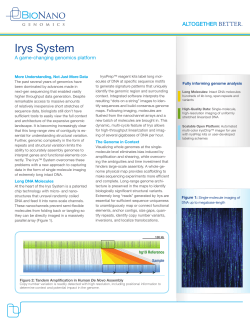
RNA Sequencing: Bottleneck
Popular assemblers diverge significantly when fed the same input
24243
448216
6457
IsoLasso
9741
7553
59647
Cufflinks
5588
Scripture
Is the bottleneck informational or computational or neither?
Source: Wei Li et al, JCB 2011, Data from ENCODE project
78
Informational Limits
• Lcritical for transcriptome assembly
No algo. can
reconstruct
Lcritical
Proposed algo. can
reconstruct in linear time
Read Length, L
0
On many examples, these two bounds match, establishing Lcritical !
• Mouse transcriptome: Lcritical = 4077 revealing complex transcriptome structure
• What can we do at practical values of L?
79
Near-Optimality at Practical L
Fraction of Transcripts Reconstructable
Read Length
Read Length
80
Near-Optimality at Practical L
Fraction of Transcripts Reconstructable
Upper bound
without
Upper
bound
on any algorithm
Upper
Bound
abundance
Read Length
Read Length
81
Near-Optimality at Practical L
Fraction of Transcripts Reconstructable
Proposed Algorithm
Read Length
Read Length
82
Necessity of Abundance Information
Fraction of Transcripts Reconstructable
Upper bound
without
abundance
Upper bound
without
abundance diversity
Read Length
Read Length
83
Transcriptome Assembly: Formulation
•
M transcripts s1,..,sM with relative abundances α1,..,αM
which are generic (rationally independent).
– Dense read model: Look at Lcrit
– Get all substrings of length L along with their relative
weights
s1
α1
s2
α2
α1+α2
αM
αM
sM
.
.
.
What is Lcritical for transcriptome?
• Lcritical is lower bounded by the length of the longest
interleaved repeat in any transcript
• It can potentially be much larger due to inter-transcript
repeats of exons across isoforms.
ATAC CAAT TCAG
GAAT TCAG
The Information Bottleneck
s1
s3
s4
s2
s3
s5
86
The Information Bottleneck
s1
s3
s4
s1
s3
s4
s2
s3
s5
s2
s3
s5
87
The Information Bottleneck
s1
s3
s4
s1
s3
s5
s2
s3
s5
s2
s3
s4
Unless L > s3 these
two transcriptomes
are confused
88
The Information Bottleneck
s1
s3
s4
s1
s3
s5
s2
s3
s5
s2
s3
s4
Sparsity can help rule out
this four transcript
alternative
But first two possibilities still
confusable unless L > s3
89
How to Distinguish the Two
s1
s3
s4
s1
s3
s5
s2
s3
s5
s2
s3
s4
90
Abundance diversity
lymphoblastoid cell line
Geuvadis dataset
Abundance Diversity
s1
s3
s4
s1
s3
s5
92
Abundance Diversity
s1
s3
s5
s1
s3
s4
s1
s3
s4
s1
s3
s5
This transcriptome is not a viable
alternative (non-uniform coverage)
Even if L < s3 these transcriptomes
are distinguishable.
93
Fooling Set under Abundance Diversity
a
s1
s2
s3
s1
s2
s4
s5
s2
s3
b
c
These two transcriptomes are still confusable if L < s2
94
Achievability: Algorithm
• From the reads
– we construct a transcript graph
Reads
0.1
ATTCG
GATTC
ATCCA
0.3
0.3
TCCAT
0.3
0.3
CCATT
CATTC
• Weight edges based on relative frequencies
95
Achievability: Algorithm
• From the reads, we construct a transcript graph
Reads
0.1
ATCCA
ATTCG
GATTC
0.3
0.3
TCCAT
0.3
0.3
CCATT
CATTC
• Weight edges based on relative frequencies
96
Achievability: Algorithm
• From the reads, we construct a transcript graph
Reads
0.1
ATC
GAT
TCG
0.3
0.3
CAT
• Weight edges based on relative frequencies
97
Transcripts from Graph
• Paths correspond to transcripts
GAT
TCG
GAT
0.1
ATC
TCG
0.3
CAT
0.3
ATC
CAT
TCG
• Naïve Algorithm: Output all paths from the
graph
98
Utility of Abundance
• Consider the following splice-graph
– Not all paths are transcripts
– Node frequencies give abundance information
0.12
s1
0.12
0.12
s4
s1
s3
s2
0.88
s3
s4
0.88
0.88
s5
s2
s3
s5
– First idea: Use continuity of copy counts
99
Utility of Abundance: Beyond Continuity
5
• More complex splice graphs:
5
12
s0
s4
7
9
7
9
s1
s3
s5
6
15
s2
s6
6
In general, we are given values on nodes /edges.
Need to find sparsest flow (on fewest paths).
100
General Splice graphs
• Principle for general splice graphs:
– Find the smallest set of paths that corresponds to the node / edge
copy counts
• Network routing, snooping, societal networks
• How to split a flow?
– Edge-flow: Flow value on each edge (satisfying conservation)
– Path-flow: Flow value on each path
– Given a edge-flow, find the sparsest path flow
0.12
0.12
s1
0.12
Start
0.12
s4
0.12
End
s3
0.88
s2
0.88
0.88
0.88
s5
0.88
101
Sparsest Flow Decomposition
• Problem is NP-Hard. [Vatinlen et al’ 08, Hartman et al
’12]
– Closer look at hard instances: most paths have same flow
– Equivalent to: Most transcripts have same abundance (!)
– This is not characteristic of the biological problem
• Our Result:
– Assume that abundances are generic
– Propose a provably correct algorithm that reconstructs
when: L > Lsuff
– Algorithm is linear time under this condition
• Approximately satisfied by biological data !
102
Iterative Algorithm
• The algorithm locally resolves paths using
abundance diversity
– Error propagation?
• Decompose a node only when sure
• If unsure, decompose other nodes before coming back to
this node
• The algorithm solves paths like a sudoku puzzle
– Solving one node can help uniquely resolve other
nodes!
– Can analyze conditions for correct recovery
• L > Lsuff
103
Algorithm: Example Run
a
a
1
a+b
1
b
a
a+b
2
b
5
46
a
a
a
47
c
b+c
a
1
b
3
2
b
2
c
35
47
3
2
34
6
34
7
1
46
b
c
b+c
5
a
7
c
b+c
5
1
6
4
3
7
c
b+c
a
4
3
2
6
5
a
1346
b
2347
c
235
104
Practical Implementation
Multibridging to construct transcript graph
Condensation and intratranscript repeat resolution
Identify and discard
sequencing errors
Aggregate abundance estimation
Node-wise copy count
estimates
Smoothing CC estimates
using min-cost network flow
Transcripts as paths
Sparsest decomposition of
edge-flow into paths
Deals with inter-transcript
repeats
Practical Performance
• Simulated reads from human chromosome
15, Gencode transcriptome
• Hard test case
•
•
•
•
•
1700 transcripts chosen randomly from Chr 15
Abundance generated from log-uniform distribution
Read length=100, 1 Million reads
1% error rates
Single-end reads / stranded protocol
106
Practical Performance
Fraction of Transcripts Missed
False Positives
1
1
0.9
0.9
0.8
0.8
0.7
0.7
0.6
0.6
0.5
Trinity
0.5
0.4
Our
0.4
0.3
0.3
0.2
0.2
0.1
0.1
0
0
1 to 10
10 to 25
25 to 50 50 to 100
Coverage Depth of Transcripts
100+
Trinity
Our
107
Complexity
• Sparsest flow problem known to be NP-Hard
– Can show using similar reduction that RNA-Seq problem under
dense reads is also NP-Hard, assuming arbitrary abundances
• Reasons why our formulation leads to poly-time
algorithm:
– Our assumption that abundances are generic
– Only worry about instances where there is enough information
– Individual sequence formulation lets us focus on issues arising
only in real genomes.
Confidence
• Can we be sure when the produced solution is correct?
– Assume dense read model
– We are finding the sparsest set of transcripts that satisfy the
given L spectrum
• Under the assumption of genericity
– Theorem: If the sparsest solution is unique, then it is the only
generic solution satisfying the L-spectrum (!)
s1
0.12
0.12
s4
0.88
s5
s3
s2
0.88
Summary
• An approach to assembly design based on principles of
information theory.
• Driven by and tested on genomics and transcriptomics
data.
• Ultimate goal is to build robust, scalable software with
performance guarantees.
Problem Landscape
measure
data
•
Assembly (de Novo)
• Noisy reads
• RNA: Finite N
• Variant calling
(reference-based
assembly)
• Indels
• Large variants
• Metagenomic
assembly
manage
data
utilize
data
• Compression
• Compress
memory?
• Genome wide
association studies
• Information
bounds
• Privacy
• Information
theoretic
methods?
• Phylogenetic tree
reconstruction
• Pathogen detection
Acknowledgements
DNA Assembly
RNA Assembly
Abolfazl Motahari
Sharif
Soheil Mohajer
Guy Bresler
MIT
Lior Pachter
Berkeley
Ma’ayan Bresler
Berkeley
Eren Sasoglu
Ka Kit Lam
Berkeley
Asif Khalak
Pacific Biosciences
Joseph Hui
Berkeley
Kayvon Mazooji
Berkeley