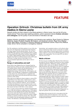
Downloaded from bmj.com on 24 September 2007
Forest plots: trying to see the wood and the trees
Steff Lewis and Mike Clarke
BMJ 2001;322;1479-1480
doi:10.1136/bmj.322.7300.1479
Updated information and services can be found at:
http://bmj.com/cgi/content/full/322/7300/1479
These include:
References
This article cites 6 articles, 1 of which can be accessed free at:
http://bmj.com/cgi/content/full/322/7300/1479#BIBL
12 online articles that cite this article can be accessed at:
http://bmj.com/cgi/content/full/322/7300/1479#otherarticles
Rapid responses
7 rapid responses have been posted to this article, which you can access for free
at:
http://bmj.com/cgi/content/full/322/7300/1479#responses
You can respond to this article at:
http://bmj.com/cgi/eletter-submit/322/7300/1479
Email alerting
service
Topic collections
Receive free email alerts when new articles cite this article - sign up in the box at
the top left of the article
Articles on similar topics can be found in the following collections
Systematic reviews (incl meta-analyses): descriptions (135 articles)
Other Statistics and Research Methods: descriptions (600 articles)
Notes
To order reprints follow the "Request Permissions" link in the navigation box
To subscribe to BMJ go to:
http://resources.bmj.com/bmj/subscribers
Downloaded from bmj.com on 24 September 2007
Education and debate
Forest plots: trying to see the wood and the trees
Steff Lewis, Mike Clarke
Few systematic reviews containing meta-analyses are
complete without a forest plot. But what are forest
plots, and where did they come from?
Summary points
Forest plots show the information from the
individual studies that went into the meta-analysis
at a glance
What is a forest plot?
In a typical forest plot, the results of component studies are shown as squares centred on the point estimate
of the result of each study. A horizontal line runs
through the square to show its confidence interval—
usually, but not always, a 95% confidence interval. The
overall estimate from the meta-analysis and its
confidence interval are put at the bottom, represented
as a diamond. The centre of the diamond represents
the pooled point estimate, and its horizontal tips
represent the confidence interval. Significance is
achieved at the set level if the diamond is clear of the
line of no effect.
The plot allows readers to see the information from
the individual studies that went into the meta-analysis
at a glance. It provides a simple visual representation of
the amount of variation between the results of the
studies, as well as an estimate of the overall result of all
the studies together. Forest plots increasingly feature in
medical journals, and the growth of the Cochrane Collaboration has seen the publication of thousands in
recent years.1
They show the amount of variation between the
studies and an estimate of the overall result
Forest plots, in various forms, have been
published for about 20 years
During this time, they have been improved, but it
is still not easy to draw them in most standard
computer packages
Neurosciences
Trials Unit,
Department of
Clinical
Neurosciences,
University of
Edinburgh, Western
General Hospital,
Edinburgh
EH4 2XU
Steff Lewis
medical statistician
UK Cochrane
Centre, NHS
Research and
Development
Programme,
Oxford OX2 7LG
Mike Clarke
associate director
(research)
Correspondence to:
S Lewis
[email protected]
nication). He based the idea on modified box plots.4
Ideas such as radial plots were also proposed.5 6
The first meta-analyses to include squares of different sizes to show the positions of the point estimates
were probably those produced by the Clinical Trial
Service Unit in Oxford in the 1998 overview of the
prevention of vascular disease by antiplatelet therapy.7
The area of each square was proportional to the weight
that the individual study contributed to the metaanalysis.
BMJ 2001;322:1479–80
History
The origin of forest plots goes back at least to the
1970s. Freiman et al displayed the results of several
studies with horizontal lines showing the confidence
interval for each study and a mark to show the point
estimate. This study was not a meta-analysis, and the
results of the individual studies were therefore not
combined into an overall result.2 In 1982, Lewis and
Ellis produced a similar plot but this time for a
meta-analysis, and they put the overall effect on the
bottom of the plot (fig 1 ).3 However, smaller studies,
with less precise estimates of effect, had larger
confidence intervals and, perversely, were the most
noticeable on the plots.
Means of focusing attention on the larger, more
precise, studies were sought. Replacement of the mark
with a square whose size was proportional to the precision of the estimate may have been first suggested by
Stephen Evans at a Royal Statistical Society medical
section meeting at the London School of Hygiene and
Tropical Medicine in 1983 (S Evans, personal commuBMJ VOLUME 322
16 JUNE 2001
bmj.com
Oxprenolol
Propranolol
Propranolol
Propranolol
Atenolol
Narrow
confidence limits
Alprenolol
Propranolol
Propranolol
Practolol
Oxprenolol
Practolol
Propranolol
Propranolol
Timolol
Metoprolol
Alprenolol
All β blockers
-300
-250
-200
-150
-100
Increase in mortality on treatment
-50
Wilcox
Norris
Multicentre
Baber
Wilcox
Andersen
Balcon
Wilcox
Barber
CPRG
Multicentre
Barber
BHAT
Multicentre
Hjalmarson
Wilhelmsson
Pooled
0
50
100%
Reduction in mortality on treatment
Fig 1 First use of forest plot for meta-analysis of effect of â blockers on mortality3
(reproduced with permission from Physicians World/Thomson Healthcare, Secaucus, NJ)
1479
Education and debate
No (%) of deaths
Study
ß blocker
Downloaded from bmj.com on 24 September 2007
ß blocker deaths
Logrank
Variance
observed of observed
Control – expected – expected
patients
Wilcox
(oxprenolol)
14/157
(8.9)
10/158
(8.9)
2.0
5.6
Norris
(propranolol)
21/226
(9.3)
24/228
(9.3)
-1.4
10.2
Multicentre
(propranolol)
15/100
(15.0)
12/95
(12.6)
1.2
5.8
Baber
(propranolol)
28/355
(7.9)
27/365
(7.4)
0.9
12.7
Andersen
(alprenolol)
61/238
(25.6)
64/242
(26.4)
-1.0
23.2
Balcon
(propranolol)
14/56
(25.0)
15/58
(25.9)
-0.2
5.5
Barber
(practolol)
47/221
(21.3)
53/228
(23.2)
-2.2
19.5
Wilcox
(propranolol)
36/259
(13.9)
19/129
(14.7)
-0.7
10.5
CPRG
(oxprenolol)
9/177
(5.1)
5/136
(3.6)
1.1
3.3
102/1533
(6.7)
127/1520
(8.4)
-13.0
53.0
Barber
(propranolol)
10/52
(19.2)
12/47
(25.5)
-1.6
4.3
BHAT
(propranolol)
138/1916
(7.2)
188/1921
(9.8)
-24.8
74.6
Multicentre
(timolol)
98/945
(10.4)
152/939
(16.2)
-27.4
54.2
Hjalmarson
(metoprolol)
40/698
(5.7)
62/697
(8.9)
-11.0
23.7
Wilhelmsson
(alprenolol)
7/114
(6.1)
14/116
(12.1)
-3.4
4.8
Total*
640/7047
(9.1)
784/6879
(11.4)
-81.6
Multicentre
(practolol)
Ratio of crude death rates (99% CI)
ß blocker: control
and they came from specially produced computer
programs. Even now, most standard statistical packages
cannot easily produce such a plot.
Why a forest plot?
The plot was not called a “forest plot” in print for some
time, and the origins of this title are obscured by
history and myth. At the September 1990 meeting of
the breast cancer overview, Richard Peto jokingly mentioned that the plot was named after the breast cancer
researcher Pat Forrest, and, at times, the name has been
spelt “forrest plot.” However, the phrase actually originates from the idea that the typical plot appears as a
forest of lines. A contender for the first use of the name
“forest plot” in print is a review of nursing
interventions for pain that was published in 1996.9 An
abstract at the Cochrane colloquium later that year
also used this name.10 We would welcome suggestions
of precedents to these uses or any other versions of this
brief history of the plot.
We thank Jon Godwin for preparing figure 2.
Funding: None.
Competing interests: None declared.
Cochrane Collaboration. Cochrane Library. Issue 1. Oxford: Update Software, 2001.
Freiman JA, Chalmers TC, Smith H, Kuebler RR. The importance of beta,
the type II error and sample size in the design and interpretation of the
randomized control trial: survey of 71 “negative trials”. N Engl J Med
1978;299:690-4.
3 Lewis JA, Ellis SH. A statistical appraisal of post-infarction beta-blocker
trials. Prim Cardiol 1982;suppl 1:31-7.
4 McGill R, Tukey JW, Larsen WA. Variations of box plots. Am Stat
1978;32:12-6.
5 DeMets DL. Methods for combining randomized clinical trials: strengths
and weaknesses. Stat Med 1987;6:341-50.
6 Galbraith RL. A note on graphical presentation of estimated odds ratios
from several clinical trials. Stat Med 1988;7:889-94.
7 Antiplatelet Trialists’ Collaboration. Secondary prevention of vascular
disease by prolonged antiplatelet treatment. BMJ 1988;296:320-31.
8 Yusuf S, Peto R, Lewis J, Collins R, Sleight P. Beta blockade during and
after myocardial infarction: an overview of the randomized trials. Prog
Cardiovasc Dis 1985;275:335-71.
9 Sindhu F. Are non-pharmacological nursing interventions for the management of pain effective? A meta-analysis. J Adv Nurs 1996;24:1152-9.
10 Bijnens L, Collette L, Ivanov A, Hoctin Boes G, Sylvester R. Optimal
graphical display of the results of meta-analyses of individual patient
data. In: Proceedings of the 4th Cochrane colloquium, Adelaide, Australia, 1996.
Oxford: Cochrane Collaboration, 1996.
1
2
310.7
0
Reduction 23.1% (SE5.0) P<0.0001
Heterogeneity between 15 trials: χ2 = 13.9; df = 14; P > 0.1
0.5
1.0
1.5
2.0
ß blocker better
ß blocker worse
Treatment effect P < 0.0001
* 95% confidence interval as shown for the odds ratio
Fig 2 Updated version of Lewis and Ellis’s original plot (fig 1 ) showing effect of â blockers
on mortality
We have updated the original Lewis and Ellis plot3
to show how it might look in the modern style (fig 2 ).
We obtained data for most of the component studies
from a subsequent paper.8 In the 1980s, no standard
computer packages could easily produce these plots,
(Accepted 20 February 2001)
A memorable patient
A chandelier and a vat of custard
It was a busy Friday night in casualty. We were one senior house
officer down and there had been a major accident on a nearby
main road. All of us had been looking after seriously injured
patients for the preceding couple of hours—not all of them had
survived, and emotions were running high. During that time, the
backlog of minor injuries had built up to a six hour wait, and
tempers were fraying in the waiting room. The nurses were
fielding angry patients, often with trivial injuries, and were
desperate for one of us to come and help.
I returned to the minor side to start clearing the backlog as
soon as possible. I was in a superefficient and slightly
short-tempered mood—didn’t they realise that we had to deal
with far more important things than cut fingers or drunks? I
picked the next card out of the box and went to the cubicle.
With barely a glance at the patient I said brusquely, “Well,
what’s the matter then?” A middle aged man looked back at me
and said, in a nonchalant tone, “I was preparing for my usual
Friday night sexual activity when the chandelier broke, and I fell
into the vat of custard.”
1480
It took a second or two for me to realise what he’d said. I
looked up at him in disbelief. “Really?” I asked. “No,” he said, “but
I’ve been sitting in the waiting room for two hours trying to pluck
up the courage to say that.”
As a grin broke over my face, I asked what had really
happened, and he told me what he had done. As I treated him, I
relaxed and chatted to him as a real person, not a patient.
I spent the rest of the shift smiling. It inspired me to think that
someone faced with a long wait had thought up something like
that, and kept it in his mind, without getting annoyed or
impatient. He changed my perspective, brightened up my
evening, and reminded me of the fact that people, not patients,
were in the waiting room.
I have long since forgotten his name, but I still think about him
when I’m having a bad day.
Katherine Whybrew GP registrar, 19 Beaumont Street Surgery,
Oxford
BMJ VOLUME 322
16 JUNE 2001
bmj.com