1. No category

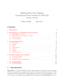
Extracting a Common Stochastic Trend:
Theories with Some Applications 1
Yoosoon Chang 2
J. Isaac Miller 3
and
Joon Y. Park 4
Abstract
This paper investigates the statistical properties of the Kalman filter for state
space models including integrated time series. In particular, we derive the full
asymptotics of maximum likelihood estimation for some prototypical class of
such models, i.e., the models with a single latent common stochastic trend.
Indeed, we establish the consistency and asymptotic mixed normality of the
maximum likelihood estimator and show that the conventional method of inference is valid for this class of models. The models considered explicitly in the
paper comprise a special, yet useful, class of models that we may use to extract
the common stochastic trend from multiple integrated time series. As we show
in the paper, the models can be very useful to obtain indices that represent
fluctuations of various markets or common latent factors that affect a set of
economic and financial variables simultaneously. Moreover, our derivation of
the asymptotics of this class makes it clear that the asymptotic Gaussianity and
the validity of the conventional inference for the maximum likelihood procedure
extends to a larger class of more general state space models involving integrated
time series. Finally, we demonstrate the utility of the state space model by extracting a common stochastic trend in three empirical analyses: interest rates,
return volatility and trading volume, and Dow Jones stock prices.
First Draft: October 2004
This version: August 2005
JEL Classification: C13, C32
Key words and phrases: state space model, Kalman filter, common stochastic trend, maximum likelihood estimation, stock price index, interest rates, return volatility and trading
volume.
1
This paper was prepared for the presentations at Symposium on Econometric Theory and Applications
(SETA) on May 18-20, 2005, at Academia Sinica, Taipei, Taiwan.
2
Department of Economics, Rice University.
3
Department of Economics, University of Missouri.
4
Department of Economics, Rice University and Sungkyunkwan University.
1
1. Introduction
The Kalman filter is perhaps one of the most widely used modeling tools, not only in econometrics and finance, but also in such diverse fields as artificial intelligence, aeronautical
engineering, and many others. Under linear, Gaussian, and stationary assumptions, the
asymptotic properties of the filter are well-known, and the technique works quite well. If
linearity is violated, then the extended Kalman filter is a standard alternative. If Gaussianity is violated, then maximum likelihood is instead pseudo-maximum likelihood. As long as
the distribution of the state (or transition) equation has a finite second moment, then the
filter retains some of its optimal properties. See Caines (1988) and Hamilton (1994) for the
statistical properties of the filter and the maximum likelihood procedure. The filter seems
to generate reasonable parameter estimates even when the distributions have thick tails, as
illustrated in Miller and Park (2004).
In this paper, we focus mainly on a violation of stationarity. Many empirical analyses
in the literature use nonstationary data or assume a nonstationary unobservable variable
or vector. The reader is referred to Kim and Nelson (1999) for an excellent survey and
many concrete examples. The properties of the Kalman filter under such assumptions,
however, are not well-known. To the best of our knowledge, no formal theory has yet been
developed for the Kalman filter applied to models with nonstationary time series. Moving
from stationary to nonstationary processes in any model calls into question rates of convergence of the parameter estimates, if not the parameter estimates themselves. Moreover,
the asymptotic theory of the maximum likelihood estimates may diverge from the standard
Gaussian framework. Consequently, a solid theoretical analysis of the Kalman filter with
nonstationary data is needed.
In this analysis, we focus on an important class of nonstationary models, i.e., models
that include integrated time series. More precisely, we consider the state space models
with a single latent common integrated stochastic trend, and analyze the properties of
the Kalman filter to estimate the parameters in these models. For this class of models, we
derive the full asymptotics of maximum likelihood estimation, and establish the consistency
and Gaussianity of the maximum likelihood estimator. The limit theories for our models
differ from the standard asymptotics for stationary models: The convergence rates are a
√
mixture of n and n, and the limit distributions are generally mixed normals. However, the
Gaussian limit distribution theory makes the conventional method of inference valid also
for our models with integrated time series. Though our theories are explicitly developed
for the simple prototypical models, it is clear that the main results in the paper extend to
more general state space models with integrated time series.
The state space models considered in the paper assume that the included time series
share one common stochastic trend. This, of course, implies that there are (m − 1)-number
of independent cointegrating relationships, if we set m to be the number of the time series
in the models. We show in the paper how our state space models are related to cointegrated
models, especially to their error correction representations. We also discuss decompositions
into the permanent and transitory components of a given time series. Our state space
models suggest a natural choice for such decompositions. However, we may also use the
decomposition based on the error correction representations of our models.
2
We consider three illustrative examples of uses of the Kalman filter to extract a common
stochastic trend. We first take on one of the most common applications in the macroeconomics literature: extracting a common trend from short- and long-term interest rates.
Subsequently, we explore an application which seems popular in the finance literature. We
look at the relationship between stock return volatility and trading volume by extracting
a common stochastic trend from those two series. In the third application, we extract the
common trend from 30 series of prices of those stocks comprising the Dow Jones Industrial
Average.
The rest of the paper is organized as follows. In Section 2, we introduce the state space
model and outline the Kalman filtering technique used to estimate the model. We also
present some preliminary results that simplify the theoretical analysis and are useful in
estimation. We present the main theoretical findings of our analysis in Section 3. Here we
analyze the maximum likelihood procedures and obtain their asymptotics. In particular,
we show that the maximum likelihood estimators are consistent and asymptotically mixed
normal. Section 4 includes some important results on the relationship between our state
space models and the usual error correction representation of cointegrated models. We
also discuss the permanent and transitory decompositions based on our models here. In
Section 5, we present the three empirical applications, and we conclude with Section 6.
Mathematical proofs of our theoretical results are contained in an Appendix.
2. The Model and Preliminary Results
We consider the state space model given by
yt = β 0 xt + u t
xt = xt−1 + vt ,
(1)
where we assume that:
(a) β0 is an m-dimensional vector of unknown parameters,
(b) (xt ) is a scalar latent variable,
(c) (yt ) is an m-dimensional observable time series,
(d) (ut ) and (vt ) are m- and 1-dimensional iid errors that are normal with mean
zero and variances Λ0 and 1, respectively, and independent of each other, and
(e) x0 is independent of (ut ) and (vt ), and assumed to be given.
The variance of (vt ) is set to be unity for the identification of β, which is identified under
this condition up to multiplication by −1. The other conditions are standard and routinely
imposed in the type of models we consider here.
Our model can be used to extract a common stochastic trend in the time series (y t ). Note
that the latent variable (xt ) is defined as a random walk, and may be regarded as a common
stochastic trend in (yt ). Here we do not introduce any dynamics in the measurement
equation, and mainly consider the simplest prototypical state space model. This is purely
for the purpose of exposition. It will be made clear that our subsequent results are directly
3
applicable for a more general class of state space models, where we have an arbitrary number
of lagged differences of the observed time series in the measurement equation.
The model given in (1) may be estimated by the usual Kalman filter. Let F t be the
σ-field generated by y1 , . . . , yt , and for zt = xt or yt , we denote by zt|s the conditional
expectation of zt given Fs , and by ωt|s and Σt|s the conditional variances of xt and yt given
Fs , respectively. The Kalman filter consists of the prediction and updating steps. For the
prediction step, we utilize the relationships
xt|t−1 = xt−1|t−1 ,
yt|t−1 = βxt|t−1 ,
and
ωt|t−1 = ωt−1|t−1 + 1,
Σt|t−1 = ωt|t−1 ββ 0 + Λ.
On the other hand, the updating step relies on the relationships
xt|t = xt|t−1 + ωt|t−1 β 0 Σ−1
t|t−1 (yt − yt|t−1 ),
2
ωt|t = ωt|t−1 − ωt|t−1
β 0 Σ−1
t|t−1 β.
The reader is referred to, e.g., Hamilton (1994) or Kim and Nelson (1999) for more details.
For any given values of β and Λ, we may show that there exist the steady state values
of ωt|t−1 and Σt|t−1 , which we denote respectively by ω and Σ. We have
Lemma 2.1
The steady state values ω and Σ exist and are given by
p
1 + 1 + 4/(β 0 Λ−1 β)
ω =
,
2
p
1 + 1 + 4/(β 0 Λ−1 β)
Σ =
ββ 0 + Λ
2
(2)
(3)
for any m-dimensional vector β and m × m matrix Λ.
From now on, we set
ω0|0 = ω − 1
(4)
so that ωt|t−1 = ω for all t ≥ 1 and becomes time invariant (and therefore, Σ t|t−1 too).
This causes no loss of generality in our asymptotic analysis, since (ω t|t−1 ) converges to its
asymptotic steady state value ω as t increases. The following lemma specifies (x t|t−1 ) more
explicitly as a function of the observed time series (y t ) and the initial value x0 . Here and
elsewhere in the paper, we assume (4). To simplify the presentation, we also make the
convention y0 = 0.
4
Lemma 2.2
We have
xt|t−1
#
"
t−1
X
β 0 Λ−1
k
(1 − 1/ω) 4yt−k + (1 − 1/ω)t−1 x0
= 0 −1
yt −
βΛ β
k=0
for all t ≥ 2.
The result in Lemma 2.2 is given entirely by our prediction and updating steps of the
Kalman filter. In particular, it holds regardless of misspecification of our model in (1).
In addition to the initial value of ω t|t−1 given by (4), we let
x0 = 0
(5)
for the rest of the paper. It is clearly seen from Lemma 2.2 that relaxing this simplifying
assumption would not affect our subsequent asymptotic analyses. Note that ω > 1, and
therefore, 0 < 1 − 1/ω < 1. Subsequently, the magnitude of the term (1 − 1/ω) t−1 x0 is
geometrically declining as t → ∞, as long as x 0 is fixed and finite a.s.
Let ω0 be the value of ω defined with the true values β 0 and Λ0 of β and Λ. If we denote
by x0t|t−1 the value of xt|t−1 under model (1), we may deduce from from Lemma 2.2 that
Proposition 2.3
We have
x0t|t−1 = xt + (1/ω0 )
t−1
X
k=1
t−1
(1 − 1/ω0 )k−1
X
β00 Λ−1
0 ut−k
(1 − 1/ω0 )k vt−k
−
−1
0
β0 Λ0 β0
k=0
for all t ≥ 2.
Proposition 2.3 implies in particular that we have
x0t|t−1 − xt = (1/ω0 )pt−1 − qt ,
where
pt =
∞
X
k=0
(1 − 1/ω0 )k
β00 Λ−1
0 ut−k
0
β0 Λ−1
0 β0
and
qt =
∞
X
k=0
(6)
(1 − 1/ω0 )k vt−k
asymptotically. If we let (ut ) and (vt ) be iid random sequences, then the time series (p t )
and (qt ) introduced in (6) become the stationary first-order autoregressive processes given
by
β00 Λ−1
0
ut
β00 Λ−1
0 β0
qt = (1 − 1/ω0 )qt−1 + vt
pt = (1 − 1/ω0 )pt−1 +
respectively. As we noted earlier, we have 0 < 1 − 1/ω 0 < 1.
Now it is clear that (x0t|t−1 ) is cointegrated with (xt ) with unit cointegrating coefficient,
i.e., (x0t|t−1 ) and (xt ) have a common stochastic trend. The stochastic trend of (x t ) may
5
therefore be analyzed by that of (x0t|t−1 ). It should be emphasized that the result in Proposition 2.3 only assumes our model specification in (1). In particular, it does not rely upon
the iid assumption on (ut ) and (vt ). Our result shows that the Kalman filter extracts the
common stochastic trend of (yt ) as long as (ut ) and (vt ) are general stationary processes,
i.e., as long as (yt ) is a vector of integrated processes. Unlike (x t ), however, (x0t|t−1 ) is not a
pure random walk, even if (ut ) and (vt ) are iid random sequences. The latter deviates from
the former up to the stationary error that is autoregressive of order one. Our results here
assume that the true parameters of the model are known. Of course, the true parameter
values are unknown and have to be estimated in most practical applications. Nevertheless, it is rather clear that our conclusions here continue to be valid as long as we use the
consistent parameter estimates.
The result in Proposition 2.3 is valid also for the state space model with the measurement
equation given by
p
X
Φk 4yt−k + ut
(7)
yt = β 0 xt +
k=1
instead of the one in (1). Under this specification, the Kalman filter has exactly the same
prediction and updating steps except for
yt|t−1 = βxt|t−1 +
p
X
k=1
Φk 4yt−k ,
replacing yt|t−1 = βxt|t−1 . Consequently, Lemma 2.1 continues to hold without modification.
Moreover,Pwe may easily obtain the result corresponding to Lemma 2.2 by substituting (y t )
by (yt − pk=1 Φk 4yt−k ), and as a result, Proposition 2.3 holds as it is. This can be seen
clearly from the proofs of Lemma 2.2 and Proposition 2.3.
3. Asymptotics for Maximum Likelihood Estimation
In this section, we consider the maximum likelihood estimation of our model. In particular,
we establish the consistency and asymptotic Gaussianity of the maximum likelihood estimator of the parameter under normality. Note that our model includes an integrated process,
and therefore, the usual asymptotic theory for the maximum likelihood estimation for the
state space model given by, for instance, Caines (1988), does not apply. We develop our
asymptotic theory in a much more general setting than the one given by our model (1) that
is explicitly considered in the paper. As will be seen clearly in what follows, our general
theory established here would be very useful to obtain the asymptotics for the maximum
likelihood estimation in a variety of models including integrated time series, both latent and
observed. Below we first develop the general asymptotic theories of maximum likelihood
estimation which allow for the presence of nonstationary time series, and then apply them
to obtain the asymptotics of the maximum likelihood estimator in our model (1).
We let θ be a κ-dimensional parameter, and define
εt = yt − yt|t−1
(8)
6
to be the prediction error with conditional mean zero and covariance matrix Σ. Under
normality, the log-likelihood function of y 1 , . . . , yn is given by
n
X
1
n
`n (θ) = − log det Σ − tr Σ−1
εt ε0t ,
2
2
t=1
(9)
ignoring the unimportant constant term. Note that Σ and (ε t ) are in general given as
functions of θ. If we denote by sn (θ) and Hn (θ) the score vector and Hessian matrix, i.e.,
sn (θ) =
∂`n (θ)
∂θ
and Hn (θ) =
∂ 2 `n (θ)
,
∂θ∂θ 0
then it follows directly from (9) that
Lemma 3.1
For the log-likelihood function given in (9), we have
1 ∂(vec Σ)0
n ∂(vec Σ)0
vec (Σ−1 ) +
vec
sn (θ) = −
2
∂θ
2
∂θ
Σ
−1
n
X
εt ε0t Σ−1
t=1
!
−
n
X
∂ε0
t
t=1
∂θ
Σ−1 εt ,
and
2
i
nh
∂
−1 0
Hn (θ) = − Iκ ⊗ vec Σ
⊗ (vec Σ)
2
∂θ∂θ 0
!0 # !
"
n
X
∂2
1
−1
0
−1
εt εt Σ
Iκ ⊗ vec Σ
⊗ (vec Σ)
+
2
∂θ∂θ 0
t=1
∂(vec Σ)
n ∂(vec Σ)0
+
Σ−1 ⊗ Σ−1
2
∂θ
∂θ 0 !
"
!
#
n
n
X
X
1 ∂(vec Σ)0
∂(vec Σ)
Σ−1 ⊗ Σ−1
−
εt ε0t Σ−1 + Σ−1
εt ε0t Σ−1 ⊗ Σ−1
2
∂θ
∂θ 0
t=1
t=1
2
n
n
X
X
∂ε0t −1 ∂εt
∂
0 −1
−
I ⊗ εt Σ
−
⊗ εt
Σ
∂θ
∂θ 0
∂θ∂θ 0
t=1
t=1
X
n n X
∂(vec Σ)
∂(vec Σ)0
∂εt
∂ε0t
−1
−1
0
+
Σ ⊗Σ
⊗ εt +
.
⊗ εt Σ−1 ⊗ Σ−1
0
∂θ
∂θ
∂θ
∂θ 0
t=1
t=1
In Lemma 3.1 and elsewhere in the paper, vec A denotes the column vector obtained by
stacking the rows of matrix A.
Denote by θˆn the maximum likelihood estimator of θ, the true value of which is denoted
by θ0 . As in the standard stationary model, the asymptotics of θˆn in our model can be
obtained from the first order Taylor expansion of the score vector, which is given by
(10)
sn (θˆn ) = sn (θ0 ) + Hn (θn ) θˆn − θ0 ,
7
where θn lies in the line segment connecting θˆn and θ0 . Of course, we have sn (θˆn ) = 0 if θˆn
is an interior solution. Therefore, it is now clear from (10) that we may write
−1 −1 0
νn0 T −1 (θˆn − θ0 ) = − νn−1 T 0 Hn (θn )T νn−10
νn T sn (θ0 )
(11)
for appropriately defined κ-dimensional square matrices ν n and T , which are introduced
here respectively for the necessary normalization and rotation.
Upon appropriate choice of the normalization matrix sequence ν n and rotation matrix
T , we will show that
ML1: νn−1 T 0 sn (θ0 ) →d N as n → ∞,
ML2: −νn−1 T 0 Hn (θ0 )T νn−10 →d M > 0 a.s. as n → ∞
for some M and N , and
ML3: There exists a sequence of invertible normalization matrices µ n such that
µn νn−1 → 0 a.s., and such that
−10 0
H
(θ)
−
H
(θ
)
T
µ
T
sup µ−1
n
n 0
n →p 0,
n
θ∈Θ0
where Θn = θ µ0n T −1 (θ − θ0 ) ≤ 1 is a sequence of shrinking neighborhoods
of θ0 ,
subsequently below.
As shown by Park and Phillips (2001) in their study of the nonlinear regression with
integrated time series, conditions ML1 – ML3 above are sufficient to derive the asymptotics
for θˆn . In fact, under conditions ML1 – ML3, we may deduce from (11) and continuous
mapping theorem that
−1 −1 0
νn T sn (θ0 ) + op (1)
νn0 T −1 (θˆn − θ0 ) = − νn−1 T 0 Hn (θ0 )T νn−10
→d M −1 N
(12)
as n → ∞. In particular, ML3 ensures that s n (θˆn ) = 0 with probability approaching to one
and
νn−1 T 0 Hn (θn ) − Hn (θ0 ) T νn−10 →p 0
as n → ∞. This was shown earlier by Wooldridge (1994) for the asymptotic analyses of
extremum estimators in models including nonstationary time series.
To derive the asymptotics for sn (θ0 ), let ε0t , (∂/∂θ 0 )ε0t and (∂/∂θ 0 )vec Σ0 be defined
respectively as εt , (∂/∂θ 0 )εt and (∂/∂θ 0 )vec Σ evaluated at the true parameter value θ 0 of
θ. We have
" n
#
n
X
X
1 ∂(vec Σ0 )0
∂ε00
t
0 00
−1
−1
sn (θ0 ) =
εt εt − Σ 0 −
Σ0 ⊗ Σ0 vec
Σ−1 ε0 ,
2
∂θ
∂θ 0 t
t=1
for which we note that
t=1
8
Remarks
0
We have ε0t = yt − yt|t−1
= β0 (xt − x0t|t−1 ) + ut . Then for sn (θ0 ) we have
(a) (ε0t , Ft ) is an mds by construction and due to (6) with conditional variance Σ 0 , and
becomes iid N(0, Σ0 ) under the assumption of normality. In particular, we have
n
1 X 0 00
√
(εt εt − Σ0 ) →d N 0, (I + K)(Σ0 ⊗ Σ0 )
n t=1
(13)
as n → ∞, where K is the commutation matrix, and
−1 0
(b) (∂/∂θ 0 )ε0t is Ft−1 -measurable, and consequently, ((∂ε 00
t /∂θ)Σ0 εt ) is an mds and
n
X
t=1
ε0t ε00
t
− Σ0
and
n
X
∂ε00
t
t=1
∂θ
0
Σ−1
0 εt
become independent asymptotically.
For the asymptotic result in (13), see, e.g., Muirhead (1982, pp.90-91).
It is now clear that the asymptotics of s n (θ0 ) can be readily deduced from our remarks
−1 0
above, if our model were stationary. Indeed, if the mds ((∂ε 00
t /∂θ)Σ0 εt ) admits the standard central limit theory (CLT), then we have as n → ∞
n
1 X ∂ε00
t
√
Σ−1 ε0 →d N(0, Ω)
n t=1 ∂θ 0 t
(14)
with the asymptotic variance Ω given by
n
∂ε0t
1 X ∂ε00
t
Σ−1
,
0
0
∂θ
∂θ
n→∞ n
t=1
Ω = plim
(15)
as is well known. The reader is referred to, e.g., Hall and Heyde (1980) for the details. Due
to the nonstationarity of our model, however, the usual CLT for the mds is not applicable
for our model, and therefore, the standard asymptotics given by (14) and (15) do not hold.
Our subsequent asymptotic theories focus on the case where (∂ε 0t /∂θ 0 ) is nonstationary, and
given by a mixture of integrated and stationary processes.
We now look at more specifically our model introduced in (1). The parameter θ in the
model is given by
θ = (β 0 , v (Λ)0 )0 ,
(16)
with the true value θ0 = (β00 , v (Λ0 )0 )0 . Here and elsewhere in the paper we use the notation
v (A) to denote the subvector of vec A with all subdiagonal elements of A eliminated. It is
well known that v (A) and vec A are related by Dv(A) = vec A, where D is the matrix called
the duplication matrix. See, e.g., Magnus and Neudecker (1988, pp.48-49). The dimension
of θ is given by κ = m + m(m + 1)/2, since in particular there are only m(m + 1)/2 number
of nonredundant elements in Λ.
For our model (1), we may easily deduce from Lemma 2.2 and Proposition 2.3 that
9
Lemma 3.2
For our model (1), we have
0
∂ε00
Λ−1
t
0 β0 β0
= − I − 0 −1
xt + at (u, v)
∂β
β0 Λ0 β0
and
∂ε00
t
= bt (u, v),
∂vecΛ
where at (u, v) and bt (u, v) are stationary linear processes driven by (u t ) and (vt ).
It is now clear from Lemma 3.2 that
∂ε00
t
=
∂θ
∂ε0t
∂ε0t
,
∂β 0 ∂v (Λ)0
0
is a matrix time series consisting of a mixture of integrated and stationary processes.
m
To further analyze the nonstationarity in (∂ε 00
t /∂θ), let εt = (εit )i=1 and consider
(∂ε0it /∂θ) individually for each i = 1, . . . , m. It is easy to see for any i = 1, . . . , m that
(∂ε0it /∂β) is an m-dimensional integrated process with a single common trend. Naturally,
there are (m − 1)-cointegrating relationships in (∂ε 0it /∂β) for each i = 1, . . . , m. There is,
however, one and only one cointegrating relationship in (∂ε 0it /∂β) that is common for all
i = 1, . . . , m, which is given by β0 . Notice that
P =I−
0
Λ−1
0 β0 β0
β00 Λ−1
0 β0
(17)
is a (m − 1)-dimensional (non-orthogonal) projection on the space orthogonal to β 0 along
0
Λ−1
0 β0 . Consequently, β0 annihilates the common stochastic trend in (∂ε it /∂β) for all
i = 1, . . . , m, and (β00 (∂ε0it /∂β)) becomes stationary for all i = 1, . . . , m. Unlike (∂ε 0it /∂β),
the process (∂ε0it /∂vecΛ) is purely stationary for all i = 1, . . . , m.
To effectively deal with the singularity of the matrix P in (17), we need to rotate the
score vector sn (θ0 ). To introduce the required rotation, we let Γ 0 be an m × (m − 1) matrix
satisfying the conditions
Γ00 Λ−1
0 β0 = 0
It is easy to deduce that
P =I−
and Γ00 Λ−1
0 Γ0 = Im−1 .
0
Λ−1
0
0 β0 β0
= Λ−1
0 Γ0 Γ0 ,
−1
0
β0 Λ0 β0
(18)
(19)
since P is a projection such that β00 P = P Λ−1
0 β0 = 0. Now we define the κ-dimensional
rotation matrix
T = (TN , TS ),
(20)
where TN and TS are matrices of dimensions κ × κ1 and κ × κ2 with κ1 = m − 1 and
κ2 = 1 + m(m + 1)/2, which are given by


β0
0
Γ0
1/2

TN =
and TS =  (β00 Λ−1
0 β0 )
0
0
Im(m+1)/2
10
respectively. We have from Lemma 3.2 and (18) and (19)
TN0
∂ε00
t
= −Γ00 xt + cN
t (u, v)
∂θ
and TS0
∂ε00
t
= cSt (u, v)
∂θ
(21)
S
for some stationary linear processes c N
t (u, v) and ct (u, v) driven by (ut ) and (vt ). Also, we
may easily deduce that


Γ00 Λ−1
0
0


β00 Λ−1
0

T −1 = 
0
(22)
 (β 0 Λ−1 β )1/2

0
0 0
0
Im(m+1)/2
from our definition of T given above in (20).
Lemma 3.3
defined by
Under our model (1), the invariance principle holds for the partial sums

[nr]
[nr]
[nr]
00
00
X
X
X
1
∂ε
∂ε
1
1
t
0
Σ−1
4TN0
TS0 t Σ−1
Un (r), Vn (r), Wn (r) =  √
,√
ε0 
0 εt , √
n
n
∂θ
n
∂θ 0 t
for r ∈ [0, 1], and we have

t=1
t=1
t=1
Un , Vn , Wn →d U, V, W ,
where U , V and W are (possiblyR degenerate) Brownian motions such that V and W are
1
0
independent of U , and such that 0 V (r)Σ−1
0 V (r) dr is of full rank a.s.
The result in Lemma 3.3 enables us to obtain the joint asymptotics of
Z 1
n
1 0 X ∂ε00
t
−1 0
V (r) dU (r),
T
Σ ε →d
n N t=1 ∂θ 0 t
0
and
(23)
n
X ∂ε00
1
t
√ TS0
Σ−1 ε0 →d W,
n t=1 ∂θ 0 t
(24)
where we denote W (1) simply by W . This convention will be made for the rest of the paper.
Note that the independence of V and U makes the limit distribution in (23) mixed Gaussian.
On the other hand, the independence of W and U renders the two limit distributions in
(23) and (24) to be independent. Clearly, we have W = d N(0, var (W )), where
!
n
0
1 X ∂ε00
t
−1 ∂εt
0
Σ
var (W ) = plim TS
TS .
(25)
n t=1 ∂θ 0 ∂θ 0
n→∞
Moreover, we may in fact represent the limit distribution in (23) as
Z 1
B2 (r) dB1 (r) Iκ1
0
11
as shown in the proof of Lemma 3.3, where B 1 and B2 are two independent univariate
standard Brownian motions.
We also have
Lemma 3.4
If we let
"
#
n
1 X 0 00
1 0 ∂(vec Σ0 )0
−1
−1
εt εt − Σ 0 ,
Σ0 ⊗ Σ0 vec √
Zn = TS
2
∂θ
n
t=1
then we have
Zn →d Z,
where Z =d N(0, var (Z)) with
1 0 ∂(vec Σ0 )0
−1
−1 ∂(vec Σ0 )
var (Z) = TS
Σ0 ⊗ Σ 0
TS ,
2
∂θ
∂θ 0
(26)
and is independent of U , V and W introduced in Lemma 3.3.
Now we are ready to derive the limit distribution for the ML estimator θ n of θ defined in
(16). It is given by (12) with the rotation matrix T in (20) and the sequence of normalization
matrix
√
(27)
νn = diag nIκ1 , nIκ2 ,
as we state below as a theorem.
Theorem 3.5 All the conditions in ML1 – ML3 are satisfied for our model (1). In
particular, ML1 and ML2 hold, respectively, with
 Z 1

−
V (r) dU (r) 
N =
0
Z −W
and
 Z
M =
1
V
0
(r)Σ−1
0 V
0
(r) dr
0
0
var (W ) + var (Z)
in notations introduced in Lemmas 3.3, 3.4, (25) and (26).
Let
and
Q=−
Z
R
S
1
V
0
(r)Σ−1
0 V
0
(r) dr
−1 Z


1
V (r) dU (r)
0
= −[var (W ) + var (Z)]−1 (W − Z),
12
where R and S are 1- and m(m + 1)/2-dimensional, respectively. Note that Q has a mixed
normal distribution, whereas R and S are jointly normal and independent of Q. Now we
may readily deduce from Theorem 3.5
√ ˇ
ˆ n ) − ˇ(Λ0 ) →d S,
n (Λ
and
h
i
ˆn − β0 ) →d Q
n(
β
Γ00 Λ−1
0
h√
i
−1
0
β0 Λ0
ˆn − β0 ) →d R.
n(
β
1/2
(β00 Λ−1
0 β0 )
(28)
(29)
In particular, it follows immediately from (28) and (29) that
√
n(βˆn − β0 ) →d
β0
R,
1/2
(β00 Λ−1
0 β0 )
(30)
ˆ n converge at the
which has degenerate normal distribution. The ML estimators βˆn and Λ
√
standard rate n, and have limit normal distributions. However, the limit distribution
of βˆn is degenerate. In the direction Γ00 Λ−1
0 , it has a faster rate of convergence n and a
mixed normal limit distribution. As will be seen in the next section, Λ −1
0 Γ0 is matrix of
cointegrating vectors for (yt ). The normal and mixed normal distribution theories of the
ML estimators ensure the standard inference to be valid for hypothesis testing in the state
space models with an integrated latent common trend. Hence, the usual t-ratios and the
asymptotic tests such as Likelihood Ratio, Lagrange Multiplier and Wald tests based on
the ML estimates are all valid and can be used in the nonstationary state space models.
It is easy to see that our asymptotic results for the maximum likelihood estimation
hold also, at least qualitatively, for the more general state space model introduced in (7).
In particular, the convergence rates, degeneracy of the limit distribution and asymptotic
Gaussianity that we establish for model (1) are also applicable for model (7). Note that Σ
is still a function of only β and Λ for more general measurement equation in (7). This is
because Lemma 2.1 is valid for model (7) as well as model (1), as we mentioned earlier in the
previous section. The additional parameters Φ 1 , . . . , Φp appearing in the lagged differenced
terms of (yt ) therefore affect the log-likelihood function in (9) only through (ε t ). Moreover,
we may observe that the first-order partial derivative of (ε t ) with respect to (Φk ) yields
(4yt−k ), with all their repeated derivatives vanishing. Consequently, it can be deduced
that the score function in Lemma 3.1 with
θ = (β 0 , vec(Φ1 )0 , . . . , vec(Φp )0 , v (Λ)0 )0
has now only additional stationary terms involving the products of (4y t−k ) and (εt ). In
particular, the presence of the additional parameters Φ 1 , . . . , Φp does not affect the nonstationary component of the score function.
13
4. Cointegration and Error Correction Representation
Our model (1) implies that (yt ) is cointegrated with the matrix of cointegrating vectors
given by an m × (m − 1) matrix Λ−1
0 Γ0 . Recall that Γ0 is the m × (m − 1) matrix satisfying
−1
0
0 −1
the condition Γ0 Λ0 β0 = 0, as defined in (18). We have Γ00 Λ−1
0 yt = Γ0 Λ0 ut , which is
stationary, and therefore Λ−1
0 Γ0 defines the matrix of cointegrating vectors of (y t ). Having
(m − 1)-number of linearly independent cointegrating relationships, (y t ) has one common
stochastic trend. Moreover, it follows from Lemma 2.2 that
Proposition 4.1
We have
4yt = −Γ0 A0 yt−1 −
t−1
X
k=1
where
A = Λ−1
0 Γ0
and Ck =
Ck 4yt−k + ε0t ,
(31)
β0 β00 Λ−1
0
(1 − 1/ω0 )k
−1
0
β0 Λ0 β0
and we follow our previous convention and use ω 0 and (ε0t ) to denote ω and (εt ) evaluated
at the true parameter value.
The result in Proposition 4.1 makes clear the relationship between our model (1) and the
usual error correction representation of a cointegrated model. Our model (1) given in state
space form differs from the conventional error correction model (ECM) in two aspects.
First, our ECM model derived from our SS model is not representable as a finite-order
vector autoregression (VAR). Here (y t ) is given as VAR(t), where the order increases with
time, and therefore it is represented as an infinite-order VAR. Second, our representation
implies that we have rank deficiencies in the short-run coefficients (C k ), as well as in the
error correction term Γ0 A0 . Note that (Ck ) are of rank one and A0 Ck = 0 for all k = 1, 2, . . ..
In the conventional ECM, on the other hand, there is no such rank restriction imposed on
the short-run coefficient matrices.
Our results in the paper for the model (1) can also be used to decompose a cointegrated
time series (yt ) into the permanent and transitory components, say (y tP ) and (ytT ), such
that
yt = ytP + ytT ,
where (ytP ) is I(1) and (ytT ) is I(0). Of course, the permanent-transitory (PT) decomposition
is not unique, and can be done in various ways. The most obvious PT decomposition based
on our model is the one given by
ytP = β0 x0t|t−1
and
ytT = yt − β0 x0t|t−1 ,
(32)
defining (x0t|t−1 ) as the common stochastic trend. The PT decomposition introduced in (32)
has the property that (ytP ) is predictable, while (ytT ) is a martingale difference sequence.
The decomposition introduced in (32) will be referred to as KF-SSM, since we use the
14
Kalman filter to extract a common trend from a state space model. Obviously, we may
estimate the common stochastic trend by (ˆ
x t|t−1 ), i.e., the values of (xt|t−1 ) evaluated at
the maximum likelihood estimates of the parameters. The transitory component can also
be estimated accordingly.
The PT decomposition proposed by Park (1990) and Gonzalo and Granger (1995) is
particularly appealing in our context. The decomposition is based on the error correction
representation of a cointegrated system, and is given by
ytP =
β0 β00 Λ−1
β0 β00 Λ−1
0 ut
0
y
=
β
x
+
t
0 t
−1
−1
0
0
β0 Λ0 β0
β0 Λ0 β0
(33)
and
0 −1
ytT = Γ0 Γ00 Λ−1
0 yt = Γ 0 Γ0 Λ0 ut .
(34)
Clearly, (ytP ) and (ytT ) defined in (33) and (34) are I(1) and I(0), respectively. They decom0 −1
pose (yt ) into two directions, i.e., β0 and Γ0 . Note that β0 β00 Λ−1
0 /β0 Λ0 β0 is the projection
on β0 along Γ0 , and that Γ0 Γ00 Λ−1
0 is the projection on Γ0 along β0 . In particular, we have
β0 β00 Λ−1
0
+ Γ0 Γ00 Λ−1
0 = I,
β00 Λ−1
β
0
0
and yt = ytP + ytT .
The directions that are orthogonal to the matrix of cointegrating vectors characterize
the long-run equilibrium path of (y t ). In fact β0 defines the direction orthogonal to the
0 −1
matrix of cointegrating vectors Λ−1
0 Γ0 since Γ0 Λ0 β0 = 0, and therefore, the shocks in the
direction of β0 lie in the equilibrium path of (yt ). This in turn implies that such shocks
do not disturb the long-run equilibrium relationships in (y t ). On the other hand, Γ0 is
the matrix of error correction coefficients as shown in Proposition 4.1, and as a result,
the shocks in the direction of Γ0 only have a transient effect. The shocks in every other
direction than the direction given by Γ 0 have a permanent effect that may interfere with
the long-run equilibrium path of (y t ), thereby distorting the long-run relationships between
the components of yt . The only permanent shocks that do not disturb the equilibrium
relationships at the outset are those in the direction of β 0 , as discussed above. The reader
is referred to Park (1990) for more details. Moreover, the decomposition given in (33)
and (34) has an important desirable property that is not present in the usual ECM: The
permanent and transitory components are independent of each other. This is because
0 −1
cov(β00 Λ−1
0 ut , Γ0 Λ0 ut ) = 0,
as one may easily check.
In our subsequent empirical applications, we also obtain the decomposition introduced
in (33) and (34). The common stochastic trend and stationary component in the decomposition are given by
0 −1
β00 Λ−1
0 yt and Γ0 Λ0 yt
respectively. These can be readily estimated using the maximum likelihood estimates of
the parameters in our model. However, to be more consistent with the methodology in
15
Park (1990) and Gonzalo and Granger (1995), we rely on the method by Johansen (1988)
and compute them using the maximum likelihood estimates of the parameters based on a
−1
finite-order ECM. Note that the estimates of the parameters Λ −1
0 β0 and Λ0 Γ0 are easily
ˆ and Aˆ respectively of Γ0 and A in ECM (31): Λ−1 β0 is a
obtained from the estimates Γ
0
vector orthogonal to Γ0 and Λ−1
0 Γ0 is given by A. In what follows, the decomposition will
be referred to as ML-ECM, in contrast to KF-SSM.
For the more general state space model with measurement equation in (7), the error
correction representation (31) in Proposition 4.1 is not valid. However, we may readily
obtain
Pa valid representation from the result in Proposition 4.1 simply by replacing (y t ) by
(yt − pk=1 Φk 4yt−k ). This is obvious from the proof of Proposition 4.1 and the discussions
in Section 2. Consequently, for t sufficiently large, we have the error correction representation of (yt ) generated by (7) that is identical to (31) with newly defined coefficients (C k ).
The coefficient A would not change. In sum, the general model (7) would have the same error correction representation as in (31) with no rank restriction in (C k ). The decomposition
in (32) and that in (33) and (34) can be defined accordingly.
5. Empirical Applications
Selection of x0|0 in applications is not as obvious as the selection of ω 0|0 discussed in Section
2. The initial value is asymptotically negligible by Lemma 2.2, but it may still have a
substantial impact on the likelihood for values of t close to zero and finite n. To this end,
Kim and Nelson (1999) and others suggest dropping some of the initial observations when
evaluating the likelihood function. We follow a two-step methodology that avoids dropping
observations in the final step. We drop some initial observations in the first step, so that
we get reasonable parameter estimates regardless of x 0|0 . Once we do this, we re-run the
estimation
with all observations and with a value of x 0|0 that is “close” to where the series
xt|t appears to begin.5 In our applications, x0|0 6= 0. By dropping initial observations,
we are dropping terms in the summation of conditional likelihoods in which t is small. The
effect of the initial condition on the remaining terms is slight. In order to avoid identification
problems, we restrict σv2 = 1 as mentioned in Section 2. To ensure positive semi-definiteness
of Λ, we estimate the Cholesky decomposition Π = (π ij ) of Λ with the restrictions πii > 0
on its diagonal elements.
In order to illustrate the uses of the KF in extracting a common stochastic trend, we
examine three well-known applications from the literature. The first two feature bivariate
(yt ), and the third features thirty-dimensional (y t ). We use a series that is smoothed according to the usual Kalman smoothing technique, rather than the unsmoothed series analyzed
above. The smoothed series utilizes information through the end of the sample. Although
this presents an advantage in empirical analysis, it necessarily complicates theoretical analysis, as (xt|n ) is defined in terms of both past and future information. Nevertheless, these
5
We do not have any
However, comparing the mag2 rigorous methodology for ascertaining “closeness”.
2
nitudes of yt − yt|t−1 for t close to zero with those of yt − yt|t−1 for t close to the end of the sample
provides a rough notion. If the magnitudes are similar at the end of the sample and at the beginning of the
sample, then x0|0 is close enough to x0 so that differences may be attributed to measurement error.
16
Figure 5.1: Log of one plus the federal funds rate and the 30-year mortgage rate (April 9, 1971 –
September 10, 2004).
series should not have noticeably different empirical characteristics. We present the PT
decompositions based on both KF-SSM and ML-ECM.
5.1 Short- and Long-Term Interest Rates
There are a number of analyses in the literature aimed at the linkage between short- and
long-term interest rates. If economic agents have rational expectations, they buy or sell
assets based on expected future interest rates. This means that the rate of return on an
asset with a longer term (long rate) is correlated with the rate of return on that of a shorter
term (short rate), since investors may choose to purchase a long-term asset or a sequence
of short-term assets. We therefore expect a stochastic trend common to rates on assets of
different terms. A more thorough discussion may be found in Modigliani and Shiller (1973)
or Sargent (1979), for example. Early theoretical analyses of cointegration and estimation
using an error correction model, such as Engle and Granger (1987), Campbell and Shiller
(1987), and Stock and Watson (1988), use this application to test the relationship between
short and long rates. More recent applied work, such as Bauwens et al. (1997) and Hafer
et al. (1997), analyze common trends among interest rates in more general international
contexts.
We extract the common stochastic trend from the federal funds rate (short rate) and
the 30-year conventional fixed mortgage rate (long rate), obtained from the Federal Reserve Bank of St. Louis (http://research.stlouisfed.org/fred2/). These series are sampled at
weekly intervals over the period April 9, 1971 through September 10, 2004, 6 and we trans6
The federal funds rate is measured on Wednesday of each week, whereas the mortgage rate is measured
on Friday of each week.
17
Figure 5.2: (a) Common stochastic trend extracted using KF-SSM; (b) Stationary components
extracted using KF-SSM; (c) Common stochastic trend extracted using ML-ECM; (d) Stationary
component extracted using ML-ECM.
form them by taking the natural logarithm of one plus the interest rate. The transformed
series are illustrated in Figure 5.1. The following table shows parameter estimates using
our technique.
Table 5.1: Parameter Estimates
Parameter
Estimate
β1
0.0008
β2
0.0011
π11
0.0191
π12
−0.0003
π22
6.0 × 10−11
from KF-SSM
Std. Error
1.1 × 10−5
1.2 × 10−5
0.0003
0.0002
3.0 × 10−5
All parameter estimates are significant except the last one. This possibly degenerate variance implies that the common trend is very similar to the long rate. This implication is
clearly visible from the trend extracted using our technique, which is represented in Figure
5.2(a), top left panel. Also, note that the more dominant of the two transitory components
[Figure 5.2(b), top right panel] more closely resembles the short rate – although it naturally
appears more stationary.
In contrast to KF-SSM, the trend extracted using ML-ECM [Figure 5.2(c), bottom left
panel] seems to more closely follow the short rate, as does the transitory component [Figure
5.2(d), bottom right panel] – at least up to a negative scale transformation. This transitory
component does not appear to be stationary.
18
Figure 5.3: (a) ρ-tests and (b) t-tests on the log of return volatility and log of trading volume with
increasing p.
5.2 Stock Return Volatility and Trading Volume
There is a large literature on the relationship between stock price volatility and trading
volume. Some notable papers among those from the 1980’s and early 1990’s include Tauchen
and Pitts (1983), Karpoff (1987), and Foster and Viswanathan (1995). These analyses
generally feature structural models intended to model some of the market microstructure
issues involved. More recent analyses, such as Fleming et al. (2004) focus on reduced form
models with one or more unobserved common factors. In light of our theoretical results in
this paper, these approaches are justified when the common factor is nonstationary. One
could conjecture that the approach is also valid with more than one common factor, but
the theoretical justification is beyond the scope of the present analysis.
In order to abstract from market microstructure issues, we look at a stock market index.
To the extent that nonlinearity enters into the model, this approach may introduce aggregation bias. Specifically, squared returns of the index may understate the actual volatility
of the individual stocks, due essentially to Schwartz’s inequality. We obtain qualitatively
similar results using KF-SSM on individual stock data, but we do not report these results.
In contrast to the interest rates considered in the previous application and to the stock
prices considered in the final application, it is not clear that stock return volatility and
transaction volume are nonstationary. As these are very noisy time series, we require
very many observations to detect nonstationarity. In this application, we examine these
measurements with respect to the Dow Jones Industrial Average (DJIA) over the period
October 2, 1928 through October 29, 2004. With weekends and holidays omitted, this daily
series obtained from Yahoo! Finance (http://finance.yahoo.com/) has 19,017 observations.
In order to detect the nonstationarity that is visibly apparent from the data, many lags must
be included in an ADF test. The short-term volatility of each series clouds the long-term
trend when the order of the ADF test is small. Figures 5.3(a) and (b) illustrate the values
of the two ADF tests, ρ-test (test based on normalized unit root coefficient) and t-test (test
based on usual t-ratio on unit root coefficient), for these two time series as the number of
19
Figure 5.4: Log of the DJIA return volatility and trading volume (November 13, 1996 – October
29, 2004).
lags increases. Nonstationarity is more apparent at higher lags.
Figure 5.4 illustrates the last 2, 000 observations of the time series (November 13, 1996
through October 29, 2004). In order to extract a common stochastic trend, we obtain the
following parameter estimates using KF-SSM.
Table 5.2: Parameter Estimates from KF-SSM
Parameter
Estimate
Std. Error
β1
0.1011
0.0013
β2
0.0231
0.0003
π11
0.1655
0.0014
π12
1.1579
0.0356
π22
2.9606
0.0184
Our trend [Figure 5.5(a), top left panel] seems to be more closely correlated with trading
volume. Since the variance parameter π 11 and coefficient β1 associated with trading volume
are relatively small and large, respectively, the stronger correlation with this series is natural.
The transitory components are illustrated in Figure 5.5(b), top right panel.
We obtain a similar stochastic trend using ML-ECM [Figure 5.5(c), bottom left panel],
although the ML-ECM trend appears more volatile. The transitory component extracted
using ML-ECM [Figure 5.5(d), bottom right panel] seems to resemble return volatility,
which we argue is not stationary.
20
Figure 5.5: (a) Common stochastic trend extracted using KF-SSM; (b) Stationary components
extracted using KF-SSM; (c) Common stochastic trend extracted using ML-ECM; (d) Stationary
component extracted using ML-ECM.
5.3 Stock Market Index
In the final application, we consider a stock market index. We wish to extract the common
stochastic trend embedded in 30 series of prices of the stocks that comprise the DJIA. We
may thus compare the common trend with the index itself. This methodology could easily
be used to extract the common stochastic trend from the prices of any set of stocks. The
novelty of this approach is that it may easily be generalized to incorporate any group of
assets. KF-SSM provides an easy way to extract a common stochastic trend or a customized
index, with weights that are optimally chosen by the algorithm. This avoids the need to
weight stocks by market capitalization or by trading volume, as some indices do.
We expect ML-ECM to fail in this application, because the parameters are estimated
using Johansen’s method. Essentially, ML-ECM is designed to extract the best trends,
with the number of trends unrestricted. KF-SSM extracts the best single trend. In twodimensional applications, such as the previous two, both approaches must extract only one
trend. In higher-dimensional applications, only one trend may be desired. In this case,
KF-SSM provides a better approach.
Gonzalo and Granger (1995) recommend dividing such a high-dimensional cointegrated
system into cohorts when analyzing with ML-ECM. 7 Essentially, those authors propose a
two-step methodology to extract a single common trend. A common trend is extracted
7
To put their recommendation in proper context, it should be noted that Gonzalo and Granger (1995)
propose the cohort approach more to justify extracting common trends from cohorts of cointegrated systems
than to actually estimate the parameters of a high-dimensional cointegrated system. They do not propose
the cohort approach as an alternative to one-step estimation.
21
Figure 5.6: Log of the DJIA (December 2, 1999 – April 7, 2004).
from the common trends that are first extracted from each of these cohorts. This reduces
the dimensionality involved in each step. Natural cohorts may be difficult to identify. For
example, in this application, it would be reasonable to group American Express, Citigroup,
and JP Morgan Chase as financial companies. But other companies such as Exxon Mobil
cannot easily be grouped with others. Moreover, with current computing power, this is
unnecessary. Calculations with a 30 × 30 matrix can be accomplished with GAUSS on a
desktop computer in a reasonable amount of time.
In this application, we use prices from Yahoo! Finance (http://finance.yahoo.com/).
These daily closing prices are adjusted to take into account stock splits and dividends
using the methodology developed by the Center for Research in Security Prices. Figure 5.6
illustrates the DJIA observed from December 2, 1999 through April 7, 2004, which is the
longest recent stretch during which the companies comprising the DJIA did not change (we
have 1, 092 observations, excluding weekends and holidays). Figure 5.7 shows the 30 series.
We include this figure to illustrate the behavioral diversity of these 30 stocks comprising
the index. It is not obvious from casual observation of these 30 series how the common
stochastic trend should look.
The implementation of KF-SSM is not as straightforward as that of ML-ECM, since
numerical optimization is required. In order to reduce the complexity and necessary computing time created by the large number of parameters, we restrict Λ to be diagonal in this
application (πij = 0 for i 6= j). This reduces the number of parameters to be estimated
using MLE from 495 to 60. Parameter estimates and standard errors for β using KF-SSM
are given in the following table.
22
Figure 5.7: Log of the 30 stocks comprising the DJIA (December 2, 1999 – April 7, 2004).
Table 5.3: Parameter Estimates from
Parameter Estimate Std. Error
β1
0.0093 5.7 × 10−5
β2
0.0080 4.6 × 10−5
β3
0.0084 5.4 × 10−5
β4
0.0088 5.1 × 10−5
β5
0.0094 7.5 × 10−5
β6
0.0087 5.1 × 10−5
β7
0.0090 5.5 × 10−5
β8
0.0087 5.0 × 10−5
β9
0.0091 5.2 × 10−5
β10
0.0087 5.0 × 10−5
β11
0.0083 4.9 × 10−5
β12
0.0085 4.8 × 10−5
β13
0.0084 4.9 × 10−5
β14
0.0090 5.2 × 10−5
β15
0.0074 4.8 × 10−5
KF-SSM
Parameter
β16
β17
β18
β19
β20
β21
β22
β23
β24
β25
β26
β27
β28
β29
β30
Estimate
0.0087
0.0082
0.0080
0.0107
0.0084
0.0084
0.0091
0.0076
0.0094
0.0080
0.0084
0.0080
0.0098
0.0093
0.0075
Std. Error
5.1 × 10−5
4.8 × 10−5
5.2 × 10−5
6.1 × 10−5
4.9 × 10−5
5.0 × 10−5
5.4 × 10−5
4.5 × 10−5
5.4 × 10−5
4.7 × 10−5
5.1 × 10−5
4.8 × 10−5
5.7 × 10−5
5.4 × 10−5
4.5 × 10−5
In the interest of brevity, we do not report parameter estimates or standard errors for the
variance parameters.
We cannot reproduce the DJIA exactly, because we restrict σ v2 = 1 for the identification
of β.8 In light of this restriction, we expect to extract a common trend resembling the
8
Alternatively, we could set σv2 equal to the variance of the differenced DJIA, which might reasonably
23
Figure 5.8: (a) Common stochastic trend extracted using KF-SSM; (b) Common stochastic trend
extracted using ML-ECM.
DJIA only up to an affine transformation. Figure 5.8(a) shows the common trend extracted
using KF-SSM, and may be directly compared with the actual DJIA shown in Figure 5.6.
The similarity suggests that KF-SSM works quite well. (We do not illustrate the transitory
components in this application, since the thirty-dimensional series generated by KF-SSM
does not contribute anything substantial to our exposition.)
Figure 5.8(b) shows the trend extracted using ML-ECM. The failure of ML-ECM to
replicate anything resembling the actual Dow Jones Industrial Average supports our intuition about the dangers of restricting the number of trends to be estimated when using that
technique. Essentially, it restricts the number of common trends after multiple trends are
extracted. Whereas, KF-SSM imposes the restriction before the trend is extracted. If the
restriction is desired – as it is in this application – KF-SSM is clearly a more appealing
approach.
6. Conclusions
The chief aim of this paper from a theoretical point of view is to justify the use of the Kalman
filter when the underlying state space model contains integrated time series. Specifically,
this class of models is useful when a single stochastic trend is common to a vector of observable cointegrated time series. Our technique is certainly not novel. The literature contains
many applications that employ the Kalman filter when the assumption of stationarity cannot be maintained. The filter seems to work reasonably well in such applications, but there
is no well-known theory to support its use in the nonstationary case. Therein lies the raison
d’ˆetre of our theoretical analysis. Our empirical applications demonstrate how our models
and theories are useful in practice.
yield a common trend more closely resembling the DJIA. However, in more general applications, no obvious
choice for σv2 exists.
24
Our research suggests many avenues for future efforts along these lines. We limit our
focus to extracting a single stochastic trend, but certainly the Kalman filter could be applied
with an unobservable vector of trends. More formal testing procedures could perhaps be
developed to test for the number of trends, as has been done for error correction models.
An advantage of the approach based on the state space models is that it does not require
nonstationarity. It is easily conceivable that a common trend with a near-unit root or an
unobservable vector with a combination of stationary and nonstationary components, for
example, could be extracted using such an approach. Although we find evidence of a unit
root in the common trend extracted from stock return volatility and trading volume, we do
not present a formal test. We leave this and other challenges for future research.
25
Mathematical Proofs
We have
Proof of Lemma 2.1
2
ωt+1|t = 1 + ωt|t−1 − ωt|t−1
β 0 Σ−1
t|t−1 β,
(35)
which follows directly from the prediction and updating steps of the Kalman filter. Moreover, we may easily deduce that
−1
−
Σ−1
t|t−1 = Λ
ωt|t−1
Λ−1 ββ 0 Λ−1 ,
1 + ωt|t−1 β 0 Λ−1 β
(36)
and therefore,
0 −1
β 0 Σ−1
t|t−1 β = β Λ β −
ωt|t−1 (β 0 Λ−1 β)2
β 0 Λ−1 β
=
.
1 + ωt|t−1 β 0 Λ−1 β
1 + ωt|t−1 β 0 Λ−1 β
(37)
Therefore, it follows from (35) and (37) that
ωt+1|t = 1 +
ωt|t−1
,
1 + ωt|t−1 β 0 Λ−1 β
(38)
which defines a first order difference equation for ω t|t−1 .
Now we may readily see that the first order difference equation in (38) has the unique
asymptotic steady state solution given in Lemma 1. For this, consider the function
f (x) = 1 +
x
1 + τx
for x ≥ 1, with any τ ≥ 0. The function has an intersection with the identity function at
p
1 + 1 + 4/τ
x=
2
over its domain x ≥ 1. Moreover, the function is monotone increasing with
f 0 (x) =
1
<1
(1 + τ x)2
for all x ≥ 1. This completes the proof for the existence of the stable value of ω t|t−1 . The
proof of Σt|t−1 follows immediately from that of ωt|t−1 .
Proof of Lemma 2.2
have
From the prediction and updating steps of the Kalman filter, we
xt+1|t = xt|t−1 + ωt|t−1 β 0 Σ−1
t|t−1 (yt − yt|t−1 )
= xt|t−1 + ωt|t−1 β 0 Σ−1
t|t−1 (yt − βxt|t−1 ).
(39)
26
However, it follows from (36) that
Σ−1 = Λ−1 −
ω
Λ−1 ββ 0 Λ−1 ,
1 + ω β 0 Λ−1 β
(40)
where Σ is the asymptotic steady state value of Σ t|t−1 given in (3). Therefore, we have from
(36)
Σ−1 β = Λ−1 β −
ω
Λ−1 ββ 0 Λ−1 β
1 + ω β 0 Λ−1 β
1
Λ−1 β,
1 + ω β 0 Λ−1 β
β 0 Λ−1 β
Λ−1 β
=
1 + ω β 0 Λ−1 β β 0 Λ−1 β
=
(41)
and
β 0 Σ−1 β = β 0 Λ−1 β −
=
ω
β 0 Λ−1 ββ 0 Λ−1 β
1 + ω β 0 Λ−1 β
β 0 Λ−1 β
.
1 + ω β 0 Λ−1 β
(42)
Moreover, we may deduce that
ω β 0 Σ−1 β =
ω β 0 Λ−1 β
1
=
1 + ω β 0 Λ−1 β
ω
(43)
due to (35).
Now we have from (39), (41), (42) and (43) that
1
1 β 0 Λ−1
yt − xt|t−1
xt+1|t = xt|t−1 +
0
−1
ωβΛ β
ω
0
1
1 β Λ−1
= 1−
yt ,
xt|t−1 +
ω
ω β 0 Λ−1 β
and consequently,
xt|t−1
t−1 1X
1 k−1 β 0 Λ−1
1 t−1
=
1−
yt−k + 1 −
x1|0 .
ω
ω
β 0 Λ−1 β
ω
(44)
k=1
Moreover,
X
t−1 t−1 1 k−1
1
1 k−1
1X
1−
yt−k = 1 − 1 −
1−
yt−k
ω
ω
ω
ω
k=1
k=1
t−2 X
1 k
1 t−1
1−
= yt −
4yt−k − 1 −
y1 .
ω
ω
(45)
k=0
The stated result now follows from (44) and (45) in a straightforward manner. Note that
x1|0 = x0|0 = x0 and y0 = 0. The proof is therefore complete.
27
Proof of Proposition 2.3 It follows from Lemma 2.2 that
#
"
t−1 X
1 k
β00 Λ−1
0
0
1−
(β0 vt−k + (ut−k − ut−k−1 ))
(β0 xt + ut ) −
xt|t−1 = 0 −1
ω0
β0 Λ0 β0
k=0
# t−1 "
t−1 −1
0
X
X
β0 Λ0
1 k
1 k
= xt + 0 −1
(ut−k − ut−k−1 ) −
vt−k(.46)
ut −
1−
1−
ω0
ω0
β0 Λ0 β0
k=0
k=0
However, we may easily deduce that
t−1 X
k=0
1
1−
ω0
k
t−1 1 X
1 k−1
(ut−k − ut−k−1 ) = ut −
ut−k .
1−
ω0
ω0
(47)
k=1
The stated result now follows readily from (46) and (47).
Proof of Lemma 3.1 The proof just requires the standard rules of differentiation, and
the details are therefore omitted.
Proof of Lemma 3.2 In the proof, we use the generic notation w t to signify any stationary linear process driven by (u t ) and (vt ). In particular, the definition of w t is different
from line to line. Due to Lemma 2.2, we may write
xt|t−1 =
β 0 Λ−1
yt + w t .
β 0 Λ−1 β
(48)
for all values of β and Λ. Moreover, we may readily deduce that
∂xt|t−1
ββ 0 Λ−1
Λ−1
I − 2 0 −1
yt + w t
= 0 −1
∂β
βΛ β
βΛ β
∂xt|t−1
Λ−1 β ⊗ Λ−1
ββ 0 Λ−1
= −
I − 0 −1
yt + w t
∂vecΛ
β 0 Λ−1 β
βΛ β
(49)
(50)
for all values of β and Λ. As a consequence, if we use the superscript “0” to denote the
derivative ∂xt|t−1 /∂θ evaluated at the true parameter values consistently with our earlier
notations, then we have
∂x0t|t−1
∂β
Λ−1 β0
= − 0 0 −1 xt + wt
β0 Λ0 β0
and
∂x0t|t−1
∂vecΛ
= wt .
(51)
We now note that
∂x0t|t−1 0
∂ε00
t
= −x0t|t−1 I −
β
∂β
∂β
and
from which the stated result follows immediately.
∂x0t|t−1 0
∂ε00
t
=−
β,
∂vecΛ
∂vecΛ
28
Proof of Lemma 3.3
It follows follow immediately from (21) that
Vn (r) =
1
−Γ00 √
n
[nr]
X
vt + op (1).
t=1
Moreover, due to (21), TS0 (∂ε00
t /∂θ) is a stationary linear process. Moreover, it is F t−1 measurable. Consequently, Wn is a partial sum process of the martingale difference sequence
−1 0
TS0 (∂ε00
t /∂θ)Σ0 εt . The stated results can therefore be readily deduced from the invariance
principle for the martingale difference sequence.
To deduce the stated result, we simply note that
"
#
n
X
−1
∂(vec Σ0 )0
−1 1
0 00
vec Σ0 √
ε ε − Σ 0 Σ0
∂θ
n t=1 t t
"
#
n
1 X 0 00
∂v (Σ0 )0 0 −1
−1
D Σ0 ⊗ Σ0 vec √
=
ε ε − Σ0
∂θ
n t=1 t t
∂v (Σ0 )0 0 −1
D Σ0 ⊗ Σ−1
N
0,
(I
+
K)(Σ
⊗
Σ
)
→d
0
0
0
∂θ
0
∂v (Σ0 )
−1
=d
N 0, 2D 0 Σ−1
D
0 ⊗ Σ0
∂θ
∂(vec Σ0 )0
−1
N 0, 2 Σ−1
.
=d
0 ⊗ Σ0
∂θ
Proof of Lemma 3.4
Here we use the fact
KD = D,
as shown in, e.g., Magnus and Neudecker (1988, p.49).
Proof of Theorem 3.5 The proof will be done in three steps, for each of ML1 – ML3. In
the proof, we use the following notational convention:
(a) (wt ) denotes a linear process driven by (u s )ts=1 and (vs )ts=1 that has geometrically decaying coefficients, and
(b) (w t ) is such a process that is Ft -measurable.
The notations wt and wt are generic and signify any processes satisfying the conditions
specified above. In general, wt and w t appearing in different lines represent different processes.
29
First Step We have
"
#
n
0
X
1
1 0
∂(vec
Σ
)
1
0
−1
T sn (θ0 ) = √ TN0
vec √
Σ−1
ε0 ε00 − Σ0
0 ⊗ Σ0
n N
2 n
∂θ
n t=1 t t
n
−
= −
= −
→d −
1 X 0 ∂ε00
TN t Σ−1
ε0
n
∂θ 0 t
1
n
Z
t=1
n
X
TN0
t=1
1
∂ε00
t
Σ−1 ε0 + Op (n−1/2 )
∂θ 0 t
Vn (r) dUn (r) + op (1)
0
Z
1
V (r) dU (r)
(52)
0
as n → ∞. On the other hand, we may deduce that
"
#
n
1 X 0 00
1 0 ∂(vec Σ0 )0
1 0
−1
−1
√ TS sn (θ0 ) = TS
Σ0 ⊗ Σ0 vec √
ε ε − Σ0
n
2
∂θ
n t=1 t t
n
1 X 0 ∂ε00
t
T
−√
Σ−1 ε0
n t=1 S ∂θ 0 t
= Zn − Wn
→d Z − W
(53)
as n → ∞. Consequently, it follows from (52) and (53) that ML1 holds with N given in the
theorem.
Second Step Next we establish ML2. First, we note that
!
n
0
∂ε
1 0 X ∂ε00
1 0
t
T Hn (θ0 )TN = − 2 TN
Σ−1 t TN + Op (n−1 )
n2 N
n
∂θ 0 ∂θ 0
t=1
Z 1
0
Vn (r)Σ−1
= −
0 Vn (r) dr + op (1)
0
Z 1
0
V (r)Σ−1
→d −
0 V (r) dr
(54)
0
as n → ∞, and that
1
n3/2
TN0 Hn (θ0 )TS = Op (n−1/2 )
(55)
30
for large n, which are in particular due to
n
X
∂2
0
I⊗
⊗ εt = Op (n)
∂θ∂θ 0
t=1
n X
∂ε0t
∂(vec Σ0 )0
−1
−1
0
Σ0 ⊗ Σ 0
⊗ εt = Op (n)
∂θ
∂θ 0
t=1
n X
∂ε0t 0
−1 ∂(vec Σ0 )
00
Σ−1
⊗ εt
= Op (n)
0 ⊗ Σ0
∂θ
∂θ 0
t=1
−1
ε00
t Σ0
for large n.
Secondly, we show that
1 0
T Hn (θ0 )TS →p var (W ) + var (Z),
n S
(56)
which establishes ML2, together with (54) and (55). To derive (56), we first write
1 0
T Hn (θ0 )TS = A + Bn + Cn + (Dn + Dn0 ),
n S
(57)
where
A =
Bn =
Cn =
Dn =
1 0 ∂(vec Σ0 )0
−1
−1 ∂(vec Σ0 )
− TS
Σ0 ⊗ Σ 0
TS
2
∂θ
∂θ 0
n
0
1 X 0 ∂ε00
t
−1 ∂εt
TS
TS
Σ
−
n
∂θ 0 ∂θ 0
t=1
2
n
1X 0
∂
00 −1
0
−
TS
⊗ εt
TS I ⊗ ε t Σ0
n
∂θ∂θ 0
"t=1
#
n 0
X
∂ε0t
−1 1
0 ∂(vec Σ0 )
−1
0
TS .
TS
Σ0 ⊗ Σ 0
⊗ εt
∂θ
n
∂θ 0
t=1
As shown earlier, we have
A = var (Z)
and Bn = var (W ) + op (1).
Moreover, since
TS0
(58)
∂ε00
t
= w t−1 ,
∂θ
we have
Dn =
for large n.
TS0
"
n
X
∂(vec Σ0 )0
−1 1
Σ−1
0 ⊗ Σ0
∂θ
n t=1
∂ε0t
TS ⊗ ε0t
∂θ 0
#
= Op (n−1/2 )
(59)
31
Now it suffices to show that
Cn (β, β) Cn (β, Λ)
Cn =
= Op (n−1/2 ),
Cn (Λ, β) Cn (Λ, Λ)
(60)
since (56) follows immediately from (57) – (60). For the subsequent proof, it will be very
useful to note that
∂xt|t−1
xt|t−1 + β 0
= wt−1
∂β
for all β and Λ. Therefore, we have upon differentiating with respect to β and Λ
2
∂xt|t−1
0 ∂ xt|t−1
+
β
= w t−1
∂β 0
∂β∂β 0
2
∂xt|t−1
0 ∂ xt|t−1
+
β
= w t−1 ,
∂(vec Λ)0
∂β∂(vec Λ)0
2
(61)
(62)
which hold for all β and Λ.
For (60), we first prove
n
1X 0
∂2
0
00 −1
Cn (β, β) =
⊗ εt
β0 = Op (n−1/2 ).
β0 (I ⊗ εt Σ0 )
n
∂β∂β 0
t=1
This can be easily derived, since we have
∂
∂ε00
∂2
t
0
β0
⊗ ε t β0 =
vec
∂β∂β 0
∂β 0
∂β
"
#
∂x0t|t−1
∂ 2 x0t|t−1
∂x0t|t−1
= −(vec I)
−
⊗ β0 −
⊗ I β0
∂β 0
∂β∂β 0
∂β
!
"
#
∂x0t|t−1
∂ 2 x0t|t−1
∂x0t|t−1
β0 I +
β0 β00 +
= −vec
β00
∂β 0
∂β∂β 0
∂β
!
#
"
∂x0t|t−1
∂x0t|t−1
β0 I −
β00 + w t−1 ,
= −vec
∂β 0
∂β
and it follows that
∂2
0
0
00 −1
⊗ εt
β0
β0 (I ⊗ εt Σ0 )
∂β∂β 0
!
"
#
∂x0t|t−1
∂x0t|t−1
0
0
0
0
0
β0 I −
= −β0
β0 Σ−1
0 εt + w t−1 εt = w t−1 εt ,
∂β 0
∂β
from which we may deduce (63), upon noticing
n
X
t=1
wt−1 ε0t = Op (n1/2 )
(63)
32
for large n.
Similarly, we have for any vector λ of conformable dimension
∂2
∂
∂ε00
t
0
⊗ εt λ =
vec
λ
∂β∂(vec Λ)0
∂(vec Λ)0
∂β
#
"
∂ 2 x0t|t−1
∂x0t|t−1
−
⊗ β0 λ
= −(vec I)
∂(vec Λ)0 ∂β∂(vec Λ)0
"
!
#
∂x0t|t−1
∂ 2 x0t|t−1
0
= −vec
λ I+
λβ ,
∂(vec Λ)0
∂β∂(vec Λ)0 0
and it follows that
∂2
0
00 −1
0
β0 (I ⊗ εt Σ0 )
⊗ εt
λ
∂β∂(vec Λ)0
#
!
"
∂ 2 x0t|t−1
∂x0t|t−1
0
0
λ I+
λβ 0 Σ−1
= −β00
0 εt = w t−1 εt ,
∂(vec Λ)0
∂β∂(vec Λ)0 0
as was to be shown. The proof for Cn (Λ, Λ) is straightforward, since
∂x0t|t−1
∂vec Λ
= w t−1
and
∂ 2 x0t|t−1
∂vec Λ∂(vec Λ)0
= w t−1 .
(64)
This can be easily deduced after some tedious but straightforward algebra. The proof for
ML2 with given M is therefore complete.
Third Step To establish ML3, we let
µn = νn1−δ
for some δ > 0 small, and let θ ∈ Θn be arbitrarily chosen. Since
−1+δ
)
Γ00 Λ−1
0 (β − β0 ) = O(n
β00 Λ−1
0
(β − β0 ) = O(n−1/2+δ ),
−1
0
1/2
(β0 Λ0 β0 )
we may set
β = β0 + n−1/2+δ β0 + n−1+δ Γ0
Λ = Λ0 + n
without loss of generality.
−1/2+δ
I
(65)
(66)
33
We will show that
1
T0
2(1−δ) N
"
n X
∂ε0
∂ε00
− t
∂θ
∂θ
t
∂ε0t
Σ−1
0
0
#
TN →p 0
∂θ
#
00 0
0
1
∂ε
∂ε
∂ε
∂ε
t
t
TN →p 0
− t Σ−1
− t0
T0
0
∂θ
∂θ 0
∂θ
n2(1−δ) N t=1 ∂θ
" n #
00
0
X ∂ε0
1
∂ε
∂ε
t
t
T0
− t Σ−1
TS →p 0
0
n1−δ S t=1 ∂θ
∂θ
∂θ 0
2
n
−1 ∂
1 X 0
0
0
00
⊗ εt
TS I ⊗ εt − ε t Σ0
TS →p 0
n1−δ
∂θ∂θ 0
t=1
2
n
1 X 0
∂
00 −1
0
TS →p 0
I ⊗ ε t Σ0
⊗ εt − ε t
T
n1−δ t=1 S
∂θ∂θ 0
"
#
n 0
1 X
∂εt ∂ε0t
−1
−1
0 ∂(vec Σ0 )
0
Σ0 ⊗ Σ 0
TS
− 0 ⊗ εt
TS →p 0
∂θ
n1−δ
∂θ 0
∂θ
t=1
"
#
n 0
0
X
∂ε
1
∂(vec
Σ
)
0
t
−1
TS →p 0
⊗ εt − ε0t
Σ−1
TS0
0 ⊗ Σ0
∂θ
n1−δ
∂θ 0
n
t=1
" n X
(67)
(68)
(69)
(70)
(71)
(72)
(73)
t=1
and
"
n X
∂ε0
#
0
∂ε
∂ε
t
TS →p 0
(74)
T0
− t0
Σ−1
0
n1−δ S t=1
∂θ 0
∂θ
2
n
−1 1 X 0
∂
0
00
0
⊗ εt − ε t
TS I ⊗ εt − ε t Σ0
TS →p 0
(75)
n1−δ
∂θ∂θ 0
t=1
"
#
n 0
1 X
∂εt
∂ε0t
−1
−1
0 ∂(vec Σ0 )
0
TS
− 0 ⊗ εt − ε t
Σ0 ⊗ Σ 0
TS →p 0 (76)
∂θ
n1−δ t=1
∂θ 0
∂θ
1
∂ε00
t
− t
∂θ
∂θ
for all β and Λ satisfying (65) and (66).
Here we only prove that the nonstationary components in (67) – (76) satisfy the required conditions. It is rather obvious that the required conditions hold for the stationary
components. In what follows, we use the generic notation ∆(n κ xt ) to denote the terms
which include nκ (or of a lower order) times (xt ). Clearly, we have
εt − ε0t ,
∂2
∂ε0t ∂ε00
⊗ εt − ε0t = ∆(n−1/2+δ xt ) + wt ,
− t ,
0
∂θ
∂θ ∂θ∂θ
(77)
since both β = β0 + O(n−1/2+δ ) and Λ = Λ0 + O(n−1/2+δ ). The results in (67) – (73) follow
immediately from (77).
The proofs for (74) – (76) are more involved. For (75) and (76), we need to show
x0t|t−1 = xt + wt
xt|t−1 − x0t|t−1
= −n
−1/2+δ
(78)
xt ∆(n
−1+2δ
xt ) + w t .
(79)
34
The result in (78) follows directly from (48). To establish (79), note that
xt|t−1 −
x0t|t−1
=
∂x0t|t−1
∂β 0
(β − β0 ) +
∂x0t|t−1
∂(vec Λ)0
(vec Λ − vec Λ0 ) + ∆(n−1+2δ xt ) + wt
= −n−1/2+δ xt + ∆(n−1+2δ xt ) + wt
due to (51). Now it follows immediately from (78) and (79) that
εt − ε0t = −(β − β0 )x0t|t−1 − β xt|t−1 − x0t|t−1 = ∆(n−1+2δ xt ) + wt ,
(80)
from which, together with (77), we may easily deduce (75) and (76).
Finally, we prove (74). To do so, we first show that
β00
β00
∂x0t|t−1
∂β
∂x0t|t−1
∂xt|t−1
−
∂β
∂β
!
= −xt + wt
(81)
= 2n−1/2+δ xt + ∆(n−1+2δ xt ) + wt .
(82)
The result in (81) follows immediately from (51). To derive (82), we note that
0
∂ 2 x0t|t−1
∂ 2 x0t|t−1
∂xt|t−1 ∂xt|t−1
−
=
(β − β0 ) +
(vec Λ − vec Λ0 )
∂β
∂β
∂β∂β 0
∂β∂(vec Λ)0
+ ∆(n−1+2δ xt ) + wt ,
and that
β00
∂ 2 x0t|t−1
∂β∂β 0
= −2β00
∂x0t|t−1
∂β 0
(β − β0 ) + wt
and β00
∂ 2 x0t|t−1
∂β∂(vec Λ)0
= wt ,
(83)
which follow from (51), (61) and (62). Consequently, we have
0
∂x0t|t−1
∂εt ∂ε00
t
0
= − xt|t−1 − x0t|t−1 β00 − β00
β0
−
(β − β0 )0
∂β
∂β
∂β
!
∂x0t|t−1
∂xt|t−1
0
β0
−
− β0
∂β
∂β
= n−1+2δ xt + wt ,
(84)
due to (79), (81) and (82).
Moreover, we have
∂x0t|t−1
∂xt|t−1
−
∂vec Λ
∂vec Λ
∂ 2 x0t|t−1
∂ 2 x0t|t−1
=
(β
−
β
)
+
(vec Λ − vec Λ0 ) + ∆(n−1+2δ xt ) + wt
0
∂vec Λ∂β 0
∂vec Λ∂(vec Λ)0
= ∆(n−1+2δ xt ) + wt ,
(85)
35
due to (64) and (83). Consequently, it follows directly from (85) that
!
0
∂x0t|t−1
∂xt|t−1 ∂xt|t−1
∂ε0t
∂ε00
t
−
= −
−
(β − β0 )0
β0 −
∂vec Λ ∂vec Λ
∂vec Λ
∂vec Λ
∂vec Λ
= ∆(n−1+2δ xt ) + wt .
(86)
Now (84) and (86) yield (74), and the proof is complete.
Proof of Proposition 4.1 The stated result follows immediately from Lemma 2.2 and
the result in (19). Note that we have from Lemma 2.2
#
"
t−1
X
β0 β00 Λ−1
k
0
0
(1 − 1/ω0 ) 4yt−k
yt −
β0 xt|t−1 = 0 −1
β0 Λ0 β0
k=0
under the convention (5), and the stated result may now be easily derived using (19) and
β0 x0t|t−1 = yt − ε0t ,
which is due to the definition of (ε0t ).
References
Anderson, B.D.O. and J.B. Moore (1979). Optimal Filtering. Englewood Cliffs, N.J.:
Prentice Hall.
Bauwens, L., D. Deprins, and J.-P. Vandeuren (1997). “Modelling Interest Rates with a
Cointegrated VAR-GARCH Model,” Discussion Paper 9780, CORE.
Campbell, J.Y. and R.J. Shiller (1987). “Cointegration and Tests of Present Value Models,” The Journal of Political Economy, 95, 1062-88.
Caines, P.E. (1988). Linear Stochastic Systems. New York, N.Y.: John Wiley & Sons.
Engle, R.F. and C.W.J. Granger (1987). “Co-Integration and Error Correction: Representation, Estimation, and Testing,” Econometrica, 55, 251-76.
Fleming, J., C. Kirby, and B. Ostdiek (2004). “Stochastic Volatility, Trading Volume, and
the Daily Flow of Information,” Journal of Business, forthcoming.
Foster, F.D. and S. Viswanathan (1995). “Can Speculative Trading Explain the VolumeVolatility Relation?” Journal of Business and Economic Statistics, 13, 379-96.
Gonzalo, J. and C.W.J. Granger (1995). “Estimation of Common Long-Memory Components in Cointegrated Systems,” Journal of Business & Economic Statistics, 13,
27-35.
36
Hafer, R.W., A.M. Kutan, and S. Zhou (1997). “Linkage in EMS Term Structures: Evidence from Common Trend and Transitory Components,” Journal of International
Money and Finance, 16, 595-607.
Hai, W., N.C. Mark and Y. Wu (1997). “Understanding spot and forward exchange rate
regressions,” Journal of Applied Econometrics, 12, 715-734.
Hall, P. and C.C. Heyde (1980). Martingale Limit Theory and Its Application. New York,
N.Y.: Academic Press.
Hamilton, J.D. (1994). Time Series Analysis. Princeton, N.J.: Princeton University Press.
Johansen, S. (1988). “Statistical Analysis of Cointegration Vectors,” Journal of Economic
Dynamics and Control, 12, 231-54.
Karpoff, J.M. (1987). “The Relation Between Price Changes and Trading Volume: A
Survey,” The Journal of Financial and Quantitative Analysis, 22, 109-26.
Kim, C.-J. and C.R. Nelson (1999). State-Space Models with Regime Switching. Cambridge, M.A.: MIT Press.
Magnus, J.R. and H. Neudecker (1988). Matrix Differential Calculus. Chichester, U.K.:
John Wiley & Sons.
Miller, J.I. and J.Y. Park (2004). “Nonlinearity, Nonstationarity, and Thick Tails: How
They Interact to Generate Persistency in Memory,” mimeographed, Department of
Economics, Rice University.
Modigliani, F. and R. J. Shiller (1973). “Inflation, Rational Expectations and the Term
Structure of Interest Rates,” Economica, 40, 12-43.
Muirhead, R.J. (1982). Aspects of Multivariate Statistical Theory. New York, N.Y.: John
Wiley & Sons.
Park, J.Y. (1990). “Disequilibrium Imputs Analysis,” mimeographed, Department of Economics, Cornell University.
Park, J.Y. and P.C.B. Phillips (2001). “Nonlinear Regressions with Integrated Time Series,” Econometrica, 69, 117-61.
Quah (1992). “The Relative Importance of Permanent and Transitory Components: Identification and Some Theoretical Bounds,” Econometrica, 60, 107-18.
Sargent, T.J. (1979). “A Note on Maximum Likelihood Estimation of the Rational Expectations Model of the Term Structure,” Journal of Monetary Economics, 5, 133-43.
Stock, J.H. and M.W. Watson (1988). “Testing for Common Trends,” Journal of the
American Statistical Association, 83, 1097-107.
37
Stock, J.H. and M.W. Watson (1991). “A probability model of the coincidence economic indicators,” in Leading Economic Indicators: New Approaches and Forecasting Records,
ed. K. Lahiri and G.H. Moore. Cambridge, U.K.: Cambridge University Press, 63-89.
Tauchen, G.E., and M. Pitts (1983). “The Price Variability-Volume Relationship on Speculative Markets,” Econometrica, 51, 485-506.
Wooldridge, J.M. (1994). “Estimation and Inference for Dependent Processes,” in Handbook of Econometrics, Vol. IV, R.F. Engle and D.L. McFadden, ed. Amsterdam:
Elsevier, 2639-738.