1. No category

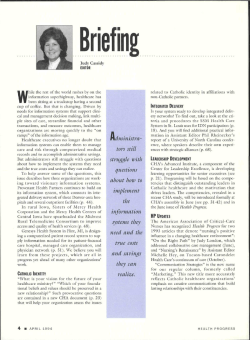
WP 14/26
Going Beyond the Mean in Healthcare Cost Regressions:
a Comparison of Methods for Estimating the Full
Conditional Distribution
Andrew M. Jones, James Lomas and Nigel Rice
August 2014
http://www.york.ac.uk/economics/postgrad/herc/hedg/wps/
Going Beyond the Mean in Healthcare Cost Regressions: a
Comparison of Methods for Estimating the Full Conditional
Distribution
Andrew M. Jones
a
a
James Lomas
a,b,∗
Nigel Rice
a,b
Department of Economics and Related Studies, University of York, YO10 5DD, UK
b
Centre for Health Economics, University of York, YO10 5DD, UK
Summary
Understanding the data generating process behind healthcare costs remains a key empirical issue. Although much research to date has focused on the prediction of the conditional
mean cost, this can potentially miss important features of the full conditional distribution
such as tail probabilities. We conduct a quasi-Monte Carlo experiment using English NHS
inpatient data to compare 14 approaches to modelling the distribution of healthcare costs:
nine of which are parametric, and have commonly been used to fit healthcare costs, and
five others designed specifically to construct a counterfactual distribution. Our results
indicate that no one method is clearly dominant and that there is a trade-off between bias
and precision of tail probability forecasts. We find that distributional methods demonstrate significant potential, particularly with larger sample sizes where the variability of
predictions is reduced. Parametric distributions such as log-normal, generalised gamma
and generalised beta of the second kind are found to estimate tail probabilities with high
precision, but with varying bias depending upon the cost threshold being considered.
JEL classification: C1; C5
Key words: Healthcare costs; heavy tails; counterfactual distributions; quasi-Monte Carlo
*Corresponding author: Tel.: +44 1904 32 1411.
E-mail address: [email protected]
1
1
Introduction
Econometric models of healthcare costs have many uses: to estimate key parameters
for populating decision models in cost-effectiveness analyses (Hoch et al., 2002); to adjust
for healthcare need in resource allocation formulae in publically funded healthcare systems
(Dixon et al., 2011); to undertake risk adjustment in insurance systems (Van de Ven and
Ellis, 2000) and to assess the effect on resource use of observable lifestyle characteristics
such as smoking and obesity (Johnson et al., 2003; Cawley and Meyerhoefer, 2012; Mora
et al., 2014). The distribution of healthcare costs poses substantial challenges for econometric modelling. Healthcare costs are non-negative, highly asymmetric and leptokurtic,
and often exhibit a large mass point at zero. The relationships between covariates and
costs are likely to be non-linear. Basu and Manning (2009) provide a useful discussion of
these issues. The relevance and complexity of modelling healthcare costs has led to the
development of a wide range of econometric approaches, and a description of these can be
found in Jones (2011).
Much of the focus in comparisons of regression methods for the analysis of healthcare
cost data has centered on predictions of the conditional mean of the distribution, E(y|X)
(Deb and Burgess, 2003; Veazie et al., 2003; Basu et al., 2004; Buntin and Zaslavsky, 2004;
Gilleskie and Mroz, 2004; Manning et al., 2005; Basu et al., 2006; Hill and Miller, 2010;
Jones, 2011; Jones et al., 2013, 2014). Applied researchers commonly model cost data using
generalised linear models (GLMs) (Blough et al., 1999). This framework offers a relatively
simple way to incorporate non-linearities in the relationship between the conditional mean
and observed covariates. Furthermore, GLMs allow for heteroskedasticity through a choice
of a ‘distribution’ which specifies the conditional variance as a function of the conditional
mean. GLMs use pseudo-maximum likelihood estimation where the researcher is required
only to specify the form of the mean and the variance. Unlike maximum likelihood estimation, where consistency requires that the whole likelihood function is correctly specified,
pseudo-maximum likelihood is consistent so long as the mean is correctly specified with the
choice of ‘distribution’ affecting the efficiency of estimates. Whilst the GLM framework
has attractive properties for researchers concerned only with E(y|X), there are important
limitations with this method. GLMs have been found to perform badly with heavy-tailed
2
data (Manning and Mullahy, 2001), and they implicitly impose restrictions on the entire
distribution. For example, whatever distribution is adopted, the skewness must be directly
proportional to the coefficient of variation and the kurtosis is linearly related to the square
of the coefficient of variation (Holly, 2009). Whilst they may be well placed to estimate
E(y|X) and V ar(y|X), they cannot produce estimates of F (y|X) or P (y > k|X).
While the mean is an important feature of a distribution, which is essential when
the analysis is concerned with the expected total cost, it is generally not the only aspect
that is of interest to policymakers (Vanness and Mullahy, 2007). Analysis based solely on
the mean misses out potentially important information in other parts of the distribution
(Bitler et al., 2006). As a result, a growing literature in econometrics has developed
techniques to model the entire distribution, F (y|X), thus ‘going beyond the mean’ (Fortin
et al., 2011). In health economics there is a particular emphasis on identifying individuals
or characteristics of individuals that lead to very large costs and there is a demand for
empirical strategies to “target the high-end parameters of particular interest” including
tail probabilities, P (y > k) (Mullahy, 2009).
In this paper we conduct a quasi-Monte Carlo experiment to compare the fit of the
entire conditional distribution of healthcare costs using competing approaches proposed in
the economics literature. We therefore consider approaches which offer greater flexibility in
terms of their potential applications by estimating F (y|X), imposing fewer restrictions on
skewness and kurtosis and allowing for a greater range of estimated effects of a covariate.
We first consider developments in the use of flexible parametric distributions for modelling healthcare costs (Manning et al., 2005; Jones et al., 2014), which have been applied
to healthcare costs principally in order to overcome the challenge posed by heavy-tailed
data. Unlike the GLM framework, these models impose a functional form for the entire
distribution with estimation by maximum likelihood. As a result, an estimate of f (y|X)
is produced, which can then be used to calculate E(y|X), V ar(y|X)1 and P (y > k|X) as
required. By using flexible distributions, the restrictions on skewness and kurtosis can be
relaxed somewhat (McDonald et al., 2013), which is likely to lead to a better fit of the full
distribution (Jones et al., 2014).
1
Note that population moments may not be defined for all ranges of parameter estimates (Mullahy,
2009).
3
A related development is the use of finite mixture models (FMM), which allow the distribution to be estimated as a weighted sum of distribution components (Deb and Trivedi,
1997; Deb and Burgess, 2003). These are also estimated using maximum likelihood, but
are often referred to as semi-parametric, since the number of components could, in principle, be increased to approximate any distribution. In this paper we group FMM with the
fully parametric distributions given the similarities to these approaches, especially since
we use a fixed number of components.
Other developments regarding the estimation of f (y|X) for healthcare costs are less
parametric, typically involving dividing the outcome variable into discrete intervals and
estimating parameters for each of these intervals. Gilleskie and Mroz (2004) propose using
a conditional density approximation estimator for healthcare costs to calculate E(y|X) and
other moments, with the density function approximated by a set discrete hazard rates. To
implement this, Jones et al. (2013) use an approach based on Han and Hausman (1990),
where F (y|X) is estimated by creating a categorical variable that denotes the cost interval
into which each observation falls, and running an ordered logit with this as the dependent
variable. This implementation is slightly different from what is proposed by Gilleskie and
Mroz (2004), but has the advantage of being conceived in order to fit F (y|X) and ties
into a related literature on semi-parametric estimators for conditional distributions (Han
and Hausman, 1990; Foresi and Peracchi, 1995; Chernozhukov et al., 2013). While the
ordered logit specification used in the Han and Hausman (1990) method allows for flexible
estimation of the thresholds in the latent scale, methods such as Foresi and Peracchi (1995)
instead estimate a series of separate logit models.
More recently, Chernozhukov et al. (2013) propose that a continuum of logits should
be estimated (one for each unique value of the outcome variable) to allow for an even
greater range of estimates for the effect of a covariate. In an application to Dutch health
expenditures, de Meijer et al. (2013) use the Chernozhukov et al. (2013) method to decompose changes in the distribution of health expenditures between two periods. The
authors find that the effect of covariates varies across the distribution of health expenditures, which would have been missed if analysis had focused solely on the mean. They
also find that pharmaceutical costs are growing mainly at the top of the distribution due
to structural effects, whereas growth in hospital care costs is observed more in the mid4
dle of the distribution and can be explained by changes in the observed determinants of
expenditure.
The methods described above seek to estimate the full distribution, by modelling
F (y|X) for different values of y (interval thresholds) and imposing varying degrees of
flexibility on the covariate effects for these. An alternative is to construct F (y|X) through
the inverse of the distribution function, the quantile function qτ (X).2 We consider two
methods which estimate a range of quantiles separately as functions of the covariates to
allow for flexibility as to the estimated effects of each regressor across the full range of
the distribution. The first was proposed by Machado and Mata (2005) and Melly (2005)
and uses a series of quantile regressions to estimate the full range of quantiles across
the distribution (hereafter MM method). Quantile regressions have been used where the
outcome variable was healthcare costs for analysing the varying effects of race at different
points of the distribution (Cook and Manning, 2009). However we were unable to find
any applications of the MM method to construct a complete estimate of F (y|X) with
healthcare costs as the outcome variable, although the applications in the original papers
were to wages, which share similar distributional characteristics. Quantile functions can
alternatively be estimated using recentred-influence-function (RIF) regression (Firpo et al.,
2009), where the outcome variable is first transformed according to the recentred-influencefunction and then regression used to model the effects of covariates.
This paper provides a systematic comparison of parametric and distributional methods3 for fitting the full distribution of healthcare costs using real data in a quasi-Monte
Carlo experiment. As such, it is novel in two ways: firstly, it provides a methodology
for comparing the distributional fit of models which are neither special cases nor estimated using the same procedure, and secondly it is the first paper to compare competing
econometric approaches for modelling the distribution of healthcare costs. We find that
distributional methods demonstrate significant potential in modelling tail probabilities,
particularly with larger sample sizes where the variability of predictions is reduced. Parametric distributions such as log-normal, generalised gamma and generalised beta of the
second kind are found to estimate tail probabilities with high precision, but with varying
2
3
τ ∈ (0, 1) denotes the quantile being considered.
This term was used in Fortin et al. (2011).
5
bias depending upon the cost threshold being considered.
The study design is described in the next section, followed by a detailed description
of the methods compared. We then discuss the results, and place these in the context
of related research, and remark upon some of the limitations of our study and possible
extensions for future work.
2
Methodology and Data
2.1
Overview
Rather than comparing competing approaches for estimating E(y|X), which is the
focus of most empirical work in this area (Mullahy, 2009), we assess performance in terms
of tail probabilities, P (y > k), for varying levels of k to assess the fit of the entire distribution, F (y|X). We compare a number of different regression methods, each with a different
number of estimated parameters. Since more complex methods may capture idiosyncratic
characteristics of the data as well as the systematic relationships between the dependent
and explanatory variables, there is a concern that better fit will not necessarily be replicated when the model is applied to new data (Bilger and Manning, 2014). To guard against
this affecting our results, we use a quasi-Monte Carlo design where models are fitted to a
sample drawn from an ‘estimation’ set and performance is evaluated on a ‘validation’ set.
This means that methods are assessed when being applied to new data.4 Each method
is used to produce an estimate of the whole distribution F (y|X), which can then be used
to produce a counterfactual distribution given the covariates in the ‘validation’ set. We
evaluate performance based on forecasting tail probabilities, P (y > k).5
2.2
Data
Our data comes from the English administrative dataset, Hospital Episode Statistics
(HES)6 , for the financial year 2007-2008. We have excluded spells which were primarily
4
There are substantial precedents for using split-sample methods to evaluate different regression methods for healthcare costs, for example Duan et al. (1983); Manning et al. (1987).
5
The values of k are not used in estimating the distribution F (y|X).
6
HES is maintained by the NHS Information Centre, now known as the Health and Social Care Information Centre.
6
mental or maternity healthcare and all spells taking place within private sector hospitals.7
The remaining spells constitute the population of all inpatient episodes, outpatient visits
and A&E attendances that were completed within 2007-2008 for all patients who were
admitted to English NHS hospitals (where treatment was not primarily mental or maternity healthcare). Spells are costed using tariffs from 2008-20098 by applying the relevant
tariff to the most expensive episode within the spell (where a spell can be thought of as a
discrete admission).9 Our analysis is undertaken at the patient level and so we sum the
costs in all spells for each patient to create the dependent variable, giving us 6,164,114
observations in total. The empirical density and cumulative distribution of the outcome
variable can be seen in Figure 1 and descriptive statistics are found in Table 1.10
N
Mean
Median
Standard deviation
Skewness
Kurtosis
Minimum
Maximum
> £500
> £1, 000
> £2, 500
> £5, 000
> £7, 500
> £10, 000
6, 164, 114
£2, 610
£1, 126
£5, 088
13.03
363.18
£217
£604, 701
% observations
82.96%
55.89%
27.02%
13.83%
6.92%
4.09%
% of total costs
97.20%
89.80%
72.35%
54.65%
38.67%
29.35%
Table 1: Descriptive statistics for hospital costs
In order to tie in with existing literature on comparisons of econometric methods for
healthcare costs, we use a set of morbidity characteristics which we keep constant for
each regression method. In addition, we control for age and sex using an interacted,
cubic specification, which leaves us with a set of regressors similar to a simplified resource
7
This dataset was compiled as part of a wider project considering the allocation of NHS resources
for secondary care services. Since a lot of mental healthcare is undertaken in the community and with
specialist providers, and hence not recorded in HES, the data is incomplete. In addition, healthcare budgets
for this type of care are constructed using separate formulae. Maternity services are excluded since they
are unlikely to be heavily determined by ‘needs’ (morbidity) characteristics, and accordingly for the setting
of healthcare budgets are determined using alternative mechanisms.
8
Reference costs for 2005-2006, which were the basis for the tariffs from 2008-2009, were used when
2008-2009 tariffs were unavailable.
9
This follows standard practice for costing NHS activity.
10
Costs above £10, 000 are excluded in these plots to make illustration clearer.
7
Figure 1: Empirical density and cumulative distribution of healthcare costs
allocation formula where health expenditures are modelled as a function of need (proxied
using detailed socio-demographic and morbidity information) (Dixon et al., 2011). In total
we use 24 morbidity markers, adapted from the ICD10 chapters (WHO, 2007), which are
coded as one if one or more spells occur with any diagnosis within the relevant subset of
ICD10 chapters (during the financial year 2007-2008) and zero otherwise.
To give some illustration of the features of the data conditional upon these covariates
we construct an index using these regressors and divide the data from the ‘estimation’
set into five quantiles (quintiles) according to the value of the index.11 For each quintile
we display the empirical distribution of log-costs12 in Figure 2, and in particular pick out
those that exceed ln(£10, 000). It is clear from Figure 2 that the conditional distributions
of log-costs (and thus costs) vary dramatically by quintile of covariates in terms of their
shape, range and number of high cost patients, with 17% of observations with annual costs
greater than £10, 000 in the most morbid patients, compared to a population average of
4.09% (and 0.14% in the least morbid quintile). An analysis looking only at the mean of
each quintile would overlook these features of the data.
We also carry out a similar analysis, this time using untransformed costs and dividing
11
This is constructed by regressing cost against the regressors using OLS and taking the predicted cost.
A log-transformation is used to make the whole distribution easier to illustrate and P (y > k) =
P (ln(y) > ln(k)) since it is a monotonic transformation.
12
8
0.30%
0.74%
2.36%
16.89%
10
ln(10,000)
6
pop average 8
ln(healthcare costs)
12
14
0.14%
frequency by quintile according to index of covariates
%s given above are % observations with costs > £10,000 for each quintile
Figure 2: Empirical distribution of log-costs for each of the 5 quintiles of the linear index
of covariates
the ‘estimation’ set into 10 quantiles (deciles) of the linear index of covariates, where we
plot the kurtosis of each decile against its skewness. Parametric distributions impose restrictions upon possible skewness and kurtosis: one-parameter distributions are restricted
to a single point (e.g. the normal distribution imposes a skewness of 0 and a kurtosis of 3),
two-parameter distributions allow for a locus of points to be estimated, and distributions
with three or more parameters allow for spaces of possible skewness and kurtosis combinations. Figure 313 shows that the data is non-normal and provides motivation for flexible
methods, since they appear better able to model the higher moments of the conditional
distributions of the outcome variable analysed here.14 We do not represented the other
approaches used in this paper in this Figure, since the skewness and kurtosis space is not
defined for these approaches. This is because they discretise the distribution or estimate
several models, or both, and the effects on implied skewness and kurtosis is unclear.
13
Key for abbreviations: GB2 – generalised beta of the second kind, SM – Singh-Maddala, B2 – beta of
the second kind, GG – generalised gamma, LN – log-normal, WEI – Weibull.
14
A similar analysis can be found in Pentsak (2007). Note also that the lower bound of the Pearson
Type IV distribution, used in Holly and Pentsak (2006), is equal to the upper bound for the beta of the
second kind distribution (also known as Pearson Type VI).
9
DAGUMU=SMU=FISK
B2U
LOMAX
GB2U
SML=WEI
GGU=LN
1600
Full sample
1400
Quantiles
1200
Kurtosis
1000
B2L=GAMMA
800
GB2L=GGL=DAGUML
600
400
200
0
0
5
10
15
20
25
Skewness
Figure 3: Kurtosis against skewness for each of the 10 deciles of the linear index of
covariates
Note: Taken from Jones et al. (2014) and adapted from McDonald et al. (2013). The dots shown on Figure 3
were generated as follows: the data were divided into ten subsets using the deciles of a simple linear predictor for
healthcare costs using the set of regressors used in this paper. Figure 3 plots the skewness and kurtosis coefficients
of actual healthcare costs for each of these subsets, the skewness and kurtosis coefficient of the full estimation
sub-population (represented by the larger circle with cross) and theoretically possible skewness-kurtosis spaces and
loci for parametric distributions considered in the literature.
10
2.3
Quasi-Monte Carlo design
In order to fully exploit the large dataset at our disposal, before we undertake analysis
we randomly divide the 6,164,114 observations into two equally sized groups: an ‘estimation’ set and a ‘validation’ set (each with 3,082,057 observations). Because researchers
using observational data from social surveys typically have fewer observations in their
datasets than are present in our ‘estimation’ set, we draw samples from within the ‘estimation’ set. On these samples we estimate the regressions that will later be evaluated
using the ‘validation’ set data. In total we randomly draw 300 samples with replacement:
100 samples of each size Ns (Ns ∈ 5,000; 10,000; 50,000), where samples with Ns =
5,000 or 10,000 may be thought of as having a similar number of observations as small
to moderately sized datasets (Basu and Manning, 2009). We estimate 14 methods using
the outcome and regressor data from each sample, where each method can be used to
construct a counterfactual distribution of costs F (y|X) (more details on each method are
found in the Empirical Models section).
Then using all 3,082,057 observations in the ‘validation’ set, we use the covariates from
the data (but not the outcome variable) to construct F (y|X) for each method. Depending
upon which method is being considered, we can either directly obtain P (y > k|X), which
we then integrate out over values of X to produce an estimate of P (y > k), or we can
use F (y|X), which we integrate out over values of X, to give F (y), to then estimate
P (y > k). Once the estimate of P (y > k) is produced for the ‘validation’ set using either
method, it can be compared to the observed empirical proportion of costs in the data that
exceeds the threshold k.15 In this paper we choose round values for k throughout the
distribution of the outcome variable (numbers in brackets correspond to % of population
mean): k ∈ £500 (19%); £1,000 (38%); £2,500 (96%); £5,000 (192%); £7,500 (287%);
£10,000 (383%).16 Results displayed look at performance across each replication for given
method with a given sample size. We construct a ratio of predicted P (y > k) to observed
P (y > k) and look at the average of these across all replications. In addition, we analyse
15
It is worth noting that the practice of comparing observed versus empirical probabilities forms the
basis of the Andrews (1988) chi-square test, although this is designed for use with parametric methods
only, and as such is not implemented in this paper, where we are interested in the performance of both
parametric and semi-parametric approaches.
16
Table 1 gives the proportion of observations in the population that exceed these thresholds.
11
the variability of these ratios, for each method and a given sample size, using the average
absolute deviation from the average computed ratio, as well as their standard deviation
and their range.
3
Empirical models
3.1
Overview
We compare, in total, the performance of 14 different estimators, which we divide into
two groups: parametric methods and distributional methods. First we describe each of the
parametric distributions and provide its conditional probability density function – f (y|X)
– the equation to calculate P (y > k|X), as well as the procedure for integrating over X in
order to produce an estimate of P (y > k). For the remaining five methods, the procedure
is more varied and complex, so we provide a detailed account of the steps required to
produce estimates of P (y > k) for all of these distributions. Table 2 provides a key for
the abbreviations used for each method throughout the remainder of the paper.
GB2 LOG
GB2 SQRT
GG
GAMMA
LOGNORM
WEIB
EXP
FMM LOG
FMM SQRT
HH
FP
CH
MM
RIF
generalised beta of the second kind (log link)
√
generalised beta of the second kind ( -link)
generalised gamma (log link)
two-parameter gamma (log link)
log-normal (log link)
Weibull (log link)
exponential (log link)
two-component finite mixture of gamma densities (log link)
√
two-component finite mixture of gamma densities ( -link)
Han and Hausman
Foresi and Peracchi
Chernozhukov, Fern´
andez-Val and Melly (linear probability model)
Machado and Mata – Melly (log-transformed outcome)
recentered-influence-function regression (linear probability model)
Table 2: Key for method labels
3.2
Parametric methods
All nine of the parametric approaches that we consider, including two variants of finite
mixture models17 , are estimated by specifying the full conditional distribution of healthcare costs using between one and five parameters. While it is possible in principle to allow
shape parameters to vary with covariates, preliminary work showed that this produced
17
These are elsewhere considered to be semi-parametric, since the number of components can vary, but
we fix the number of components as two, meaning that they are essentially parametric.
12
unreliable and uninterpretable results, so in all cases we only specify location parameters
as functions of covariates. This means that all models have only one parameter depending upon covariates, except FMM LOG and FMM SQRT which have scale parameters
in each component that are allowed to vary with covariates.18 All other parameters are
estimated as scalars. In Table 3 we give the conditional probability density function and
the conditional survival function for each model we compare.
18
It is also possible to specify multiple parameters as functions of regressors to allow for more complex
covariate effects.
13
Model
f (y|X) =
P(y > k|X) =
GB2 LOG
ay ap−1
y
ap
exp (Xβ) B(p,q)[1+( exp (Xβ)
)a ](p+q)
1 − IZ (p, q)* where z =
GB2 SQRT
ay ap−1
(Xβ)2ap B(p,q)[1+(
1 − IZ (p, q)* where z =
GG
κ
σyΓ(κ−2 )
GAMMA
LOGNORM
WEIB
EXP
FMM LOG
14
FMM SQRT
y
)a ](p+q)
(Xβ)2
κ−2
κ−2
κ/σ
y
exp (Xβ)
−2
κ
y
1
κ−2 exp (Xβ)
yΓ(κ−2 )
−(ln y−Xβ)2
1
√
exp
2σ 2
σy 2π
1
σy
y
exp (Xβ)
1
σ
exp −
j
πj
exp −κ−2
y αj
yΓ(αj )(Xβj )2αj
κ/σ
y
exp (Xβ)
y
exp (Xβ)
1 exp −
ln k−Xβ
σ
exp −
exp −
y
exp (Xβ
j )
y
(Xβj )2
k
exp (Xβ)
k
exp − exp (Xβ)
κ > 0: 1 − Γ z; κ−2 ** if κ < 0:Γ z; κ−2 ** where z = κ−2
σ
a
k
exp (Xβ)
a
k
2
(Xβ)
if κ > 0: 1 − Γ z; κ−2 ** if κ < 0: Γ z; κ−2 ** where z = κ−2
1−Φ
R z tp−1
1
B(p,q) 0 (1+t)p+q dt is the incomplete
R
−2
**where Γ z; κ−2 = Γ(κ1−2 ) 0z t(κ −1) exp (−t)dt.
1 R z (αj −1)
***where Γ (z; αj ) = Γ(α
t
exp (−t)dt.
j) 0
*where IZ (p, q) =
y
exp (Xβ)
−y
1
exp (Xβ) exp (Xβ)
P2
y αj
j πj yΓ(αj ) exp (Xβj )αj
P2
exp −κ−2
1 σ
P2
j
πj (1 − Γ (z; αj ))*** where z =
k
exp (Xβj )
P2
πj (1 − Γ (z; αj ))*** where z =
k
(Xβj )2
j
beta function ratio.
Table 3: Forms of density functions and survival functions for parametric distributions
k
exp (Xβ)
k
exp (Xβ)
κ/σ
The generalised beta of the second kind19 is a four-parameter distribution that was
applied to modelling healthcare costs by Jones (2011) specifying the location parameter as a linear function of covariates using software developed by Jenkins (2009). Jones
et al. (2014) estimated the distribution with a log link (GB2 LOG) making it more comparable with commonly used approaches. With this specification, for example, GG (as
proposed by Manning et al., 2005) becomes a limiting case of GB2 LOG. Jones et al.
(2013) also compared GB2 SQRT as well as GB2 LOG against a broad range of models,
finding that the GB2 SQRT performed particularly well in terms of accurately predicting
mean individual healthcare costs. GG has been compared more extensively in terms of
predicting mean healthcare costs, having been found to out-perform a GLM log link with
gamma-distribution in the presence of heavy tails using simulated data (Manning et al.,
2005), and a number of models within the GLM framework when a log link is appropriate
using American survey data; the Medical Expenditures Panel Survey (Hill and Miller,
2010). GB2 LOG, GG and LOGNORM are compared in Jones et al. (2014), with some
indication that GB2 LOG better fits the entire distribution with lower AIC and BIC, although LOGNORM better predicts tail probabilities associated with the majority of high
costs considered. We also consider further special cases of GG (and GB2 LOG) with two
parameters (GAMMA and WEIB) and with one parameter (EXP).
Finite mixture models have been used in health economics in order to allow for heterogeneity both in response to observed covariates and in terms of unobserved latent
classes (Deb and Trivedi, 1997). Heterogeneity is modelled through a number of components, denoted C, each of which can take a different specification of covariates (and
shape parameters, where specified), written as fj (y|X), with an associated parameter for
the probability of belonging to each component, πj . The general form of the probability
density function of finite mixture models is given as:
f (y|X) =
C
X
πj fj (y|X)
(1)
j
We use two gamma-distributed components in our comparison.20 In one of the models
19
Also known as generalised-F, see Cox (2008).
Preliminary work showed that models with a greater number of components lead to problems with
convergence in estimation. Empirical studies such as Deb and Trivedi (1997) provide support for the two
components specification for healthcare use.
20
15
used, we allow for log links in both components (FMM LOG), and in the other we allow
for a square root link in both components (FMM SQRT). In both, the probability of
class membership is treated as constant for all individuals. Unlike the other parametric
methods, this approach can allow for a multi-modal distribution of costs. In this way, finite
mixture models represent a flexible extension of parametric models (Deb and Burgess,
2003). Using increasing numbers of components, it is theoretically possible to fit any
distribution, although in practice researchers tend to use few components (two or three)
and achieve good approximation to the distribution of interest (Heckman, 2001).
Once we have obtained estimates of location parameters (all βs for each regressor)
and shape parameters for each distribution, these are stored in memory and then used
to generate estimates of P (y > k|X), where values for X are the observed covariates in
the ‘validation’ set. These estimated conditional tail probabilities will vary across each
possible combination of X, and hence for any given individual i, and so we take the average
in order to ‘integrate out’ these to provide us with a single estimate of P (y > k) for each
method and replication, which can be compared to the proportion of costs empirically
observed to exceed k. We then take the average across all replications of P (y > k) for
each method in order to assess bias and analyse the variability across replications as an
indicator of precision.
3.3
Distributional methods
3.4
Methods using the cumulative distribution function
Of the remaining five methods that we compare, three involve estimation of the conditional distribution function and two operate through the quantile function. First we
consider the methods which estimate the conditional distribution function F (y|X). Han
and Hausman (1990) adopts a proportional hazards specification, where the baseline hazard is allowed to vary non-parametrically across a number, denoted DHH , of intervals
of a discretised continuous outcome variable. The logarithm of the integrated baseline
hazard for each of the DHH − 1 intervals (one is arbitrarily omitted for estimation) is
estimated as a constant δDHH . The effects of covariates are estimated using a particular
functional form, which is typically linear. This approach is similar to the semi-parametric
16
Cox proportional hazard model (Cox, 1972), but differs in that the baseline hazard is not
regarded as a nuisance parameter and is better suited to data with many ties of the outcome variable (or in the case of a discrete outcome). In order to implement this method,
we construct a categorical variable for each observation, indicating the interval into which
the value of the outcome variable falls. This is then used as the dependent variable in
an ordered logit regression on the covariates. The cut-points are estimates of the baseline
hazard within each interval δDHH . The authors argue that given a large sample size, finer
intervals should improve the efficiency of the estimator, without providing guidance on a
specific number of intervals to be used. As a result we carried out preliminary work to
establish the largest number of intervals that could be used for each sample size whilst
maintaining good convergence performance,21 which resulted in a maximum of 33 intervals
for sample sizes 5,000 and 10,000, and 36 intervals for a sample size of 50,000.
Foresi and Peracchi’s (1995) method is similar to Han and Hausman’s (1990) in that
it divides the data into a set of discrete intervals. Rather than using an ordered logit
specification, Foresi and Peracchi (1995) estimate a series of logit regressions. For each
upper boundary of the DF P − 1 intervals (the highest value interval is excluded), an
indicator variable is created which is equal to one if the observation’s observed cost is
less than or equal to the upper boundary, and zero otherwise. These are then used as
dependent variables in DF P − 1 logit regressions each using the full set of regressors. In
their application to excess returns in their paper they use zero, as well as the 10th, 15th,
20th, ... , 80th, 85th and 90th percentiles as boundaries. While we do not have information
on patients with zero costs in our dataset, we base our intervals on their specification of
the dependent variables by using the 5th, 10th, 15th, ... , 85th, 90th and 95th percentiles
(vigiciles).
The third approach that we compare is an extension of Foresi and Peracchi (1995) and
is described in Chernozhukov et al. (2013). The crucial difference between the methods
is that Chernozhukov et al. (2013) argue that a logit regression should be used for each
unique value of the outcome variable. A continuum of indicator variables needs to be
generated and then regression models are used to construct the conditional distribution
functions for each value. Given the computational demand of this approach, and lack
21
This was taken to mean that the model converges at least 95 times out of the 100 samples.
17
of variation in the indicator variables at low and high costs, de Meijer et al. (2013) use
linear probability models in place of logit regressions. We also adopt this approach in our
comparison, since preliminary work showed that, where it was possible to estimate both
logit and linear probability models, there was little difference between the methods.
All of these methods are similar in that they can produce estimates of P (y > k ∗ |X),
where k ∗ represents one of the boundaries of the intervals generated using either Han and
Hausman (1990) or Foresi and Peracchi (1995), or any cost value observed in the sample
when implementing Chernozhukov et al. (2013). Since models are estimated without
knowing what thresholds (k) the policymaker might be interested in, it is not always the
case that k ∗ = k. Therefore, for all three methods described above, we use a weighted
average of P (y > k ∗ |X) for the nearest two values of k ∗ to k when k ∗ 6= k. Our weight is
based on a simple linear interpolation:
P (y > k|X) = P (y > ka∗ |X) +
k − ka∗
kb∗ − ka∗
P (y > kb∗ |X) − P (y > ka∗ |X)
(2)
where ka∗ and kb∗ represent the thresholds analysed in estimation closest below and closest
above k, respectively.22
Since we end up with an estimate for each observation of P (y > k|X), we carry out
the same procedure as with the parametric distributions. This means that we take the
average of P (y > k|X), thus ‘integrating out’ over all possible combinations of X and
giving us an estimate of P (y > k) to be compared against the empirical proportion.
3.5
Methods using the quantile function
Machado and Mata (2005) propose a method for constructing a counterfactual distribution based on a series of quantile regressions using the logged outcome variable. They
suggest that a quantile (τ ) is chosen at random by drawing from a uniform probability
distribution between zero and one. After running the quantile regression for the drawn
value, the set of estimated coefficients is used to predict the quantile given the covariate
values observed for a randomly selected observation. The authors repeat this process 4500
22
This should work well when there are a large number of k∗ spaced throughout the distribution. When
interested in high values of k this linear interpolation may be inappropriate if there are few high values of
k∗ , given the often large distances between a high cost and the next highest observed cost.
18
times with replacement, generating a full counterfactual distribution. The theoretical motivation for this procedure is that each predicted quantile based on qτ (X) represents a
draw from the conditional distribution of healthcare costs (f (y|X)). Therefore drawing a
random observation and forecasting qτ enough times with random τ effectively integrates
out X. Running such a large number of quantile regressions is computationally expensive,
and so Melly (2005) suggest running a regression for a fixed number of quantiles spread
over the full range of the distribution, e.g. for each percentile, rather than drawing a quantile at random. We use the Melly (2005) approach for the MM method, running quantile
regressions for each percentile on the ‘estimation’ set, after log-transforming the outcome
variable, and randomly choosing one of these quantiles to forecast for each observation
in the ‘validation’ set.23 Once this has been done, the forecasted values represent the
counterfactual distribution of healthcare costs belonging to the ‘validation’ set. Therefore
to produce an estimate of P (y > k) we observe the proportion of the observations in the
counterfactual distribution that exceed k.
Another method to estimate quantiles of the distribution is developed by Firpo et al.
(2009), which employs recentred-influence-function regressions. For a given observed quantile (qτ ), a recentred-influence-function (RIF) is generated, which can take one of two values depending upon whether or not the observation’s value of the outcome variable is less
than or equal to the observed quantile:
RIF (y; qτ ) = qτ +
τ − 1 [y ≤ qτ ]
fy (qτ )
(3)
Here, qτ is the observed sample (τ ) quantile, 1 [y ≤ qτ ] is an indicator variable which
takes the value one if the observation’s value of the outcome variable is less than or equal
to the observed quantile and zero otherwise, and fy (qτ ) is the estimated kernel density
of the distribution of the outcome variable at the value of the observed quantile. The
recentred-influence-function is then used as the dependent variable in an OLS regression
on the chosen covariates, which effectively constitutes a rescaled linear probability model.
These estimated coefficients can then be used to predict the quantile being analysed for
a given observation’s covariates. Following the same thought process as MM, predictions
23
The prediction is exponentiated to achieve the quantile of the distribution of the levels of healthcare
costs.
19
based on qτ (X) represent a draw from f (y|X). This means that we can use the estimated
quantile functions to predict a counterfactual distribution in the same way for the RIF
method as we do for the MM method.24
4
Results
When analysing the performance of the methods, we calculate a ratio of the estimated
P (y > k) to the actual proportion of costs in the ‘validation’ set observed to exceed
the threshold value k (see Table 4). Using a ratio allows for greater comparability when
looking at performance at different thresholds. We will look at the average ratio across
replications (with methods estimated on different samples drawn from the ‘estimation’
set25 ) as well as the variability of the ratios. The former indicates the bias associated
with each method at a given k, while the latter indicates precision of the method. First
we will look at results across methods for a given sample size and threshold cost value:
Ns = 5, 000 and k = £10, 000.26 Second we consider performance for a given sample size,
with a range of values for the threshold cost value, since different methods may be better
at fitting different parts of the distribution of healthcare costs: Ns = 5, 000 and (k ∈ £500;
£1,000; £2,500; £5,000; £7,500; £10,000). Lastly performance at different sample sizes is
evaluated at a given threshold cost value: (Ns ∈ 5,000; 10,000; 50,000) and k = £10, 000.
k
£500
£1, 000
£2, 500
£5, 000
£7, 500
£10, 000
% observations in ‘validation’ set > k
82.93%
55.89%
27.04%
13.84%
6.94%
4.10%
Table 4: Actual empirical proportion of observations greater than k in the ‘validation’ set
In Figure 4 we present the performance of the 14 methods in predicting the probability of a cost exceeding £10,000 in the validation set, when samples with Ns = 5, 000
24
We calculate the recentred-influence-function using the level of costs and so no re-transformation is
required unlike when using MM.
25
Three samples were discarded when Ns = 5, 000, due to being unable to form the categorical variable
for HH. Only one sample was discarded when Ns = 10, 000 and Ns = 50, 000.
26
We choose these values of Ns and k since they are the smallest and most challenging sample size and
the largest and most economically interesting threshold value, respectively.
20
IF
R
M
M
H
C
FP
H
H
_L
O
G
M
_S
Q
R
T
EX
P
FM
M
FM
B
EI
M
R
O
W
A
M
N
G
G
G
G
AM
LO
G
G
B2
_
LO
B2
G
_S
Q
R
T
.6
.8
1
1.2
1.4
Pr(y>£10,000): sample size 5,000
Figure 4: Performance of methods predicting the probability of a cost exceeding £10,000
at sample size 5,000
observations are used. The bars indicate the ratio of estimated to actual probability, and
the capped spikes indicate the range of ratios across all of the replications. A ratio of one
represents a perfect fit, i.e. the method correctly predicted that 4.10% of observations
would exceed £10,000.
From Figure 4, it is clear that performance of the methods varies both in terms of bias
(the point – the average ratio) and precision (the variability of ratios as depicted by the
capped spikes showing the range). There is no clear pattern in terms of parametric versus
distributional methods, since in both groups there are methods where the average ratio
is seen to be near the desired value of one, as well as methods in both groups where the
range of computed ratios does not contain one. In terms of bias, the best method is CH
with an average ratio of almost exactly one. It appears that this is not the most precise
method for k = £10, 000, however, with a range of ratios: 0.82 − 1.14, that is the fifth
largest of all methods compared (the largest belongs to FMM SQRT). To more clearly
represent the tradeoff between bias and precision, see Table 5, which gives the rankings of
each method in terms of bias (absolute value of one minus the average ratio), the range of
ratios and also the standard deviation of ratios.
21
Method
GB2 LOG
GB2 SQRT
GG
GAMMA
LOGNORM
WEIB
EXP
FMM LOG
FMM SQRT
HH
FP
CH
MM
RIF
Bias
5th
12th
9th
4th
11th
7th
10th
3rd
8th
6th
13th
1st
2nd
14th
Range
6th
5th
4th
11th
1st
12th
9th
13th
14th
7th
3rd
10th
2nd
8th
Standard deviation
6th
3rd
2nd
11th
1st
12th
8th
14th
13th
9th
4th
10th
5th
7th
Table 5: Rankings of methods based on threshold of £10,000 at sample size 5,000
From Table 5 it can be seen that three of the parametric distributions – GB2 SQRT,
GG and LOGNORM – demonstrate significant potential in terms of the variability of
their predictions as the three methods with the lowest standard deviations of ratios. MM
performs consistently well across all three measures of performance, especially when variability is measured by the range of ratios, although the standard deviation is still among
the five lowest of methods compared. From these results it is unclear which method is the
best for forecasting costs greater than £10,000, since there is no outright winner over the
three metrics.
Whilst the results outlined previously give some indication of the methods’ respective
abilities to forecast high costs, we are interested in the performance of the regression
methods at all points in the distribution. For this reason we carry out a similar analysis
across a range of cost threshold values. To present these results, once again we plot the
average ratio and the range of ratios across the replications. The results presented in
Figure 5 are undertaken using samples with 5,000 observations.
22
HH
1
.8
.6
4000
6000
8000
10000
4000
6000
8000
10000
0
2000
4000
6000
8000
10000
1.4
.6
.8
EXP
1
WEIB
1
.8
.6
2000
0
2000
4000
6000
8000
10000
0
2000
4000
6000
8000
10000
0
2000
4000
6000
8000
10000
0
2000
4000
6000
8000
10000
1.4
2000
0
1.2
0
1.2
1.4
1.2
1.4
1.2
.8
.6
10000
RIF
1
10000
8000
.8
8000
6000
.6
6000
4000
1.4
4000
2000
1.2
2000
0
MM
1
0
1.2
1.2
.8
.6
LOGNORM
1
1.2
GAMMA
1
.6
10000
.8
10000
8000
.6
8000
6000
1.4
6000
4000
1.2
4000
2000
CH
1
2000
FMM_SQRT
1
1.2
FMM_LOG
1
.8
.6
.8
GG
1
.8
0
0
.8
10000
10000
.6
8000
8000
1.4
6000
6000
1.2
4000
4000
FP
1
2000
2000
.8
0
0
.6
10000
1.4
8000
.6
.8
.6
6000
1.4
4000
1.4
1.4
1.2
1.4
GB2_SQRT
1
1.2
1.4
1.2
GB2_LOG
1
.8
.6
2000
1.4
0
Figure 5: Performance of methods predicting the probability of costs exceeding various thresholds at sample size 5,000
There is a clear pattern in Figure 5: the higher the cost threshold being considered,
the greater the variability in ratio of estimated to actual probability. Besides this, the way
in which performance varies across different thresholds, including by how much variability
increases with higher thresholds, is different for all methods.
Beginning with the parametric distributions, with log links, there seems to be little
difference in the performance of GB2 LOG and GG, except for that GB2 LOG performs
slightly better at the higher costs considered in terms of bias. Looking at the gamma-type
models, LOGNORM demonstrates potential in terms of producing precise estimates of tail
probabilities if not in terms of bias. Since FMM LOG represents a two-component version
of GAMMA, comparing the performance of these methods provides some insight into the
returns from using more complex mixture specifications. The pattern of performance at
different thresholds is quite similar for these, and the main difference seems to be that
FMM LOG produces more variable estimates, especially at low cost thresholds. WEIB
and EXP seem to perform similarly, with high variability forecasts. It is interesting to
note that the square-root link methods differ from their log link counterparts, particularly
in terms of having worse high cost forecasts.
There is considerable variation in performance between the distributional methods.
The methods that use the cumulative distribution function seem to vary predominantly
according to the number of intervals that are used, rather than the specification for predicting interval membership. CH is practically unbiased for all cost thresholds, illustrating
the strength of this method in forecasting P (y > k) for a range of values of k. As pointed
out earlier, however, the variability of the forecasts across replications is wider than the
majority of other methods considered in this paper. It seems therefore that much of the
bias in HH and FP stems from when ka∗ and kb∗ are not close to the value of k being
investigated. This is more likely to be the case with FP than with HH, since FP has fewer
intervals (and is highly unlikely using CH – in our application). This is particularly clear
with k = £10, 000, since with HH and FP in this case kb∗ will often be the highest observed
cost in the sample. When this occurs, the linear interpolation that we employ is likely to
lead to an overestimation of the forecasted probability (see equation 2 for details). For
these three methods the variability of ratios is roughly similar, but when looking also at
the methods using the quantile function, it is clear that MM offers an improvement upon
24
M
R
IF
M
FP
C
H
H
H
G
G
AM
M
A
N
O
R
M
W
EI
B
FM EX
M P
_
FM LO
G
M
_S
Q
R
T
G
G
LO
G
G
B2
_L
B2 OG
_S
Q
R
T
.6
.8
1
1.2
1.4
Pr(y>£10,000): sample size 5,000
M
IF
R
M
H
C
H
FP
H
G
G
AM
M
A
N
O
R
M
W
EI
B
FM EX
M P
_
FM LO
G
M
_S
Q
R
T
G
G
LO
G
G
B2
_L
B2 OG
_S
Q
R
T
.6
.8
1
1.2
1.4
Pr(y>£10,000): sample size 10,000
M
IF
R
M
H
C
H
FP
H
G
G
AM
M
A
N
O
R
M
W
EI
B
FM EX
M P
_
FM LO
G
M
_S
Q
R
T
G
G
LO
G
G
B2
_L
B2 OG
_S
Q
R
T
.6
.8
1
1.2
1.4
Pr(y>£10,000): sample size 50,000
Figure 6: Performance of methods predicting the probability of a cost exceeding £10,000
at different sample sizes
the variability. Its performance, however, in terms of bias varies across values of k. RIF
seems to perform badly both in terms of bias and precision.
Finally, we look into how our analysis is affected by the number of observations that
are present in the drawn samples. To do this, we return to the style of graph used for
Figure 4, but illustrate performances for the three sample sizes analysed (Ns ∈ 5,000;
10,000; 50,000). The results are therefore only for one value of k, but results at other
values followed a similar pattern.
From Figure 6 we can see that there is a clear effect of sample size on the performance of
the regression methods fitting the whole distribution. Having more observations does not
particularly affect the bias of each method, but, as expected, it reduces the variability of
the estimates. This therefore means that methods such as CH perform relatively better at
bigger sample sizes since they remain unbiased, but forecast costs with increased precision.
25
5
Discussion
The results of this paper are the first to provide a comparative assessment of paramet-
ric and distributional methods designed to estimate a counterfactual distribution. This
makes them different to most studies concerning econometric modelling of healthcare costs
where performance has largely been judged on the basis of the ability to predict conditional means. Jones et al. (2014) compare parametric distributions (but not distributional
methods) against one another for predicting tail probabilities as well as in-sample fit of the
whole distribution based on log-likelihood statistics. The analysis presented here builds
on this work with a range of thresholds for tail probabilities as well as a broader range
of parametric distributions including mixture distributions and models with a square-root
link as well as those with a log link.
As mentioned in the methodology section of the paper, some of these methods have
been automated in order to make the quasi-Monte Carlo study design feasible. For instance, we only allow location parameters to vary with covariates and we restrict the
number of mixtures used in FMM LOG and FMM SQRT. In practice, analysts are likely
to train their model for a given sample – testing the appropriateness of covariates in the
specification as well as the number of mixtures that are required etc. Since all methods
have been restricted to some degree, e.g. the regressors are the same for all methods, the
results of this paper give some indication of the relative performance of these methods and
illustrate their pitfalls and strengths.
For our application, CH demonstrates potential even for forecasting probabilities of
high costs – such as costs that exceed £10,000. A function of the methodology is that
CH (as well as HH and FP) is unable to extrapolate beyond the observed sample, and
so in applications where sample size is small, or if the decision-maker is interested in the
probability of extremely high costs beyond the largest observed, this method would be
unable to provide any information on this parameter. This represents a limitation for this
type of method for fitting the distribution of healthcare costs, where the underlying data
generating process is heavy-tailed, and any observed sample is unlikely to contain some of
the potential extreme outcomes.
There is considerable variation in the best performing parametric distributions accord-
26
ing to the specific tail probability being considered. When considering costs that exceed
£10,000, FMM LOG is the least biased parametric method, but is the most imprecise of
all methods considered. At other thresholds, the distribution with the best fit on average
varies: for example WEIB performs best among parametric distributions for costs that
exceed £7,500. This means that the preferred parametric distribution would depend upon
the decision-maker’s loss function. Some distributions are particularly imprecise at all
tails investigated, notably the mixture models – FMM LOG and FMM SQRT – as well
as some of the more restrictive distributions – GAMMA, WEIB and EXP. LOGNORM is
the most precise and thus demonstrates its potential for modelling the whole distribution
of costs. Whilst other papers have focused on the importance of the link function, which
seems to have a large impact on performance when it comes to predicting mean healthcare
costs (see for example Basu et al., 2006), this paper finds that when we are concerned with
predicting tail probabilities the link function is less of an issue than are the distributional
assumptions more generally.
The distributional methods show promise for modelling the full distribution of healthcare costs. In particular, CH is practically unbiased in terms of all forecasted tail probabilities considered. The related methods of FP and HH also perform well in terms of
bias, but not when considering costs that exceed £10,000, because £10,000 is likely to fall
in the highest quantile of costs in either method. CH is better placed to model this tail
probability, since each unique value of costs that is encountered in the sample is used as
the basis for an indicator variable for a separate regression, and using a linear probability model does not require variation across all covariates for each value of the dependent
variable. At the smallest sample size of 5,000 observations, these three methods exhibit
highly imprecise forecasted probabilities, but this becomes less of an issue at larger sample
sizes where the variability is lower for all 14 methods. MM delivers better precision, but
its performance on average varies across the different tail probabilities. RIF appears to be
the worst among the distributional methods for this dataset and specification.
Acknowledgements
The authors gratefully acknowledge funding from the Economic and Social Research
27
Council (ESRC) under grant reference RES-060-25-0045. We would also like to thank
members of the Health, Econometrics and Data Group (HEDG), at the University of
York, and John Mullahy for useful discussions.
28
References
Andrews DW. 1988. Chi-square diagnostic tests for econometric models: Introduction and
applications. Journal of Econometrics 37: 135 – 156.
Basu A, Arondekar BV, Rathouz PJ. 2006. Scale of interest versus scale of estimation:
comparing alternative estimators for the incremental costs of a comorbidity. Health
Economics 15: 1091–1107.
Basu A, Manning WG. 2009. Issues for the next generation of health care cost analyses.
Medical Care 47: S109–S114.
Basu A, Manning WG, Mullahy J. 2004. Comparing alternative models: log vs Cox
proportional hazard? Health Economics 13: 749–765.
Bilger M, Manning WG. 2014. Measuring overfitting in nonlinear models: A new method
and an application to health expenditures. Health Economics In Press.
Bitler MP, Gelbach JB, Hoynes HW. 2006. What mean impacts miss: Distributional
effects of welfare reform experiments. The American Economic Review 96: 988–1012.
Blough DK, Madden CW, Hornbrook MC. 1999. Modeling risk using generalized linear
models. Journal of Health Economics 18: 153–171.
Buntin MB, Zaslavsky AM. 2004. Too much ado about two-part models and transformation? comparing methods of modeling medicare expenditures. Journal of Health
Economics 23: 525–542.
Cawley J, Meyerhoefer C. 2012. The medical care costs of obesity: An instrumental
variables approach. Journal of Health Economics 31: 219 – 230.
Chernozhukov V, Fernndez-Val I, Melly B. 2013. Inference on counterfactual distributions.
Econometrica 81: 2205–2268.
Cook BL, Manning WG. 2009. Measuring racial/ethnic disparities across the distribution
of health care expenditures. Health Services Research 44: 1603–1621.
Cox C. 2008. The generalized F distribution: An umbrella for parametric survival analysis.
Statistics in Medicine 27: 4301–4312.
Cox DR. 1972. Regression models and life-tables. Journal of the Royal Statistical Society.
Series B (Methodological) 34: 187–220.
de Meijer C, ODonnell O, Koopmanschap M, van Doorslaer E. 2013. Health expenditure
growth: Looking beyond the average through decomposition of the full distribution.
Journal of Health Economics 32: 88 – 105.
Deb P, Burgess JF. 2003. A quasi-experimental comparison of econometric models for
health care expenditures. Hunter College Department of Economics Working Papers
212.
Deb P, Trivedi PK. 1997. Demand for medical care by the elderly: A finite mixture
approach. Journal of Applied Econometrics 12: 313–336.
29
Dixon J, Smith P, Gravelle H, Martin S, Bardsley M, Rice N, Georghiou T, Dusheiko
M, Billings J, Lorenzo MD, Sanderson C. 2011. A person based formula for allocating
commissioning funds to general practices in england: development of a statistical model.
BMJ 343: d6608.
Duan N, Manning WG, Morris CN, Newhouse JP. 1983. A comparison of alternative
models for the demand for medical care. Journal of Business & Economic Statistics 1:
115–126.
Firpo S, Fortin NM, Lemieux T. 2009. Unconditional quantile regressions. Econometrica
77: 953–973.
Foresi S, Peracchi F. 1995. The conditional distribution of excess returns: An empirical
analysis. Journal of the American Statistical Association 90: 451–466.
Fortin N, Lemieux T, Firpo S. 2011. Decomposition methods in economics. volume 4,
Part A of Handbook of Labor Economics. Elsevier, 1 – 102.
Gilleskie DB, Mroz TA. 2004. A flexible approach for estimating the effects of covariates
on health expenditures. Journal of Health Economics 23: 391–418.
Han A, Hausman JA. 1990. Flexible parametric estimation of duration and competing
risk models. Journal of Applied Econometrics 5: 1–28.
Heckman JJ. 2001. Micro data, heterogeneity, and the evaluation of public policy: Nobel
lecture. Journal of Political Economy 109: 673–748.
Hill SC, Miller GE. 2010. Health expenditure estimation and functional form: applications
of the generalized gamma and extended estimating equations models. Health Economics
19: 608–627.
Hoch JS, Briggs AH, Willan AR. 2002. Something old, something new, something borrowed, something blue: a framework for the marriage of health econometrics and costeffectiveness analysis. Health Economics 11: 415–430.
Holly A. 2009. Modeling risk using fourth order pseudo maximum likelihood methods. Institute of Health Economics and Management (IEMS), University of Lausanne, Switzerland.
Holly A, Pentsak Y. 2006. Maximum likelihood estimation of the conditional mean e(y|x)
for skewed dependent variables in four-parameter families of distribution Technical report, Institute of Health Economics and Management (IEMS), University of Lausanne,
Switzerland.
Jenkins S. 2009. GB2FIT: stata module to fit generalized beta of the second kind distribution by maximum likelihood. Statistical software components S456823. Boston
College Department of Economics.
Johnson E, Dominici F, Griswold M, L Zeger S. 2003. Disease cases and their medical
costs attributable to smoking: an analysis of the national medical expenditure survey.
Journal of Econometrics 112: 135–151.
Jones AM. 2011. Models for health care. In Clements MP, Hendry DF (eds.) Oxford
Handbook of Economic Forecasting. Oxford University Press.
30
Jones AM, Lomas J, Moore P, Rice N. 2013. A quasi-Monte Carlo comparison of developments in parametric and semi-parametric regression methods for heavy tailed and
non-normal data: with an application to healthcare costs. Health Econometrics and
Data Group Working Paper 13/30.
Jones AM, Lomas J, Rice N. 2014. Applying beta-type size distributions to healthcare
cost regressions. Journal of Applied Econometrics 29: 649–670.
Machado JAF, Mata J. 2005. Counterfactual decomposition of changes in wage distributions using quantile regression. Journal of Applied Econometrics 20: 445–465.
Manning WG, Basu A, Mullahy J. 2005. Generalized modeling approaches to risk adjustment of skewed outcomes data. Journal of Health Economics 24: 465–488.
Manning WG, Duan N, Rogers W. 1987. Monte Carlo evidence on the choice between
sample selection and two-part models. Journal of Econometrics 35: 59 – 82.
Manning WG, Mullahy J. 2001. Estimating log models: to transform or not to transform?
Journal of Health Economics 20: 461 – 494.
McDonald JB, Sorensen J, Turley PA. 2013. Skewness and kurtosis properties of income
distribution models. Review of Income and Wealth 59: 360–374.
Melly B. 2005. Decomposition of differences in distribution using quantile regression.
Labour Economics 12: 577 – 590.
Mora T, Gil J, Sicras-Mainar A. 2014. The influence of obesity and overweight on medical
costs: a panel data perspective. European Journal of Health Economics In press.
Mullahy J. 2009. Econometric modeling of health care costs and expenditures: a survey
of analytical issues and related policy considerations. Medical Care 47: S104–S108.
Pentsak Y. 2007. Addressing skewness and kurtosis in health care econometrics. PhD
Thesis, University of Lausanne.
Van de Ven WP, Ellis RP. 2000. Risk adjustment in competitive health plan markets. In
Culyer AJ, Newhouse JP (eds.) Handbook of Health Economics, volume 1 of Handbook
of Health Economics, chapter 14. Elsevier, 755–845.
Vanness DJ, Mullahy J. 2007. Perspectives on mean-based evaluation of health care. In
Jones AM (ed.) The Elgar Companion to Health Economics. Elgar Original Reference.
Veazie PJ, Manning WG, Kane RL. 2003. Improving risk adjustment for medicare capitated reimbursement using nonlinear models. Medical Care 41: 741–752.
WHO. 2007. International statistical classification of diseases and related health problems,
10th revision, version for 2007.
31
6
Appendix A
We use the variables shown in Table A1 to construct our regression models. They are
based on the ICD10 chapters, which are given in Table A2.
Variable name
epiA
epiB
epiC
epiD
epiE
epiF
epiG
epiH
epiI
epiJ
epiK
epiL
epiM
epiN
epiOP
epiQ
epiR
epiS
epiT
epiU
epiV
epiW
epiX
epiY
epiZ
Variable description
Intestinal infectious diseases, Tuberculosis, Certain zoonotic bacterial diseases, Other bacterial diseases, Infections with a predominantly sexual mode of transmission, Other spirochaetal diseases, Other diseases caused
by chlamydiae, Rickettsioses, Viral infections of the central nervous system, Arthropod-borne viral fevers and
viral haemorrhagic fevers
Viral infections characterized by skin and mucous membrane lesions, Viral hepatitis, HIV disease, Other viral
diseases, Mycoses, Protozoal diseases, Helminthiases, Pediculosis, acaiasis and other infestations, Sequelae of
infectious and parasitic diseases, Bacterial, viral and other infectious agents, Other infectious diseases
Malignant neoplasms
In situ neoplasms, Benign neoplasms, Neoplasms of uncertain or unknown behaviour and III
IV
V
VI
VII and VIII
IX
X
XI
XII
XIII
XIV
XV and XVI
XVII
XVIII
Injuries to the head, Injuries to the neck, Injuries to the thorax, Injuries to the abdomen, lower back, lumbar
spine and pelvis, Injuries to the shoulder and upper arm, Injuries to the elbow and forearm, Injuries to the
wrist and hand, Injuries to the hip and thigh, Injuries to the knee and lower leg, Injuries to the ankle and
foot
Injuries involving multiple body regions, Injuries to unspecified part of trunk, limb or body region, Effects of
foreign body entering through natural orifice, Burns and Corrosions, Frostbite, Poisoning by drugs, medicaments and biological substances, Toxic effects of substances chiefly nonmedicinal as to source, Other and
unspecified effects of external causes, Certain early complications of trauma, Comlications of surgical and
medical care, not elsewhere classified, Sequelae of injuries, of poisoning and of other consequences of external
causes
XXII
Transport accidents
Falls, Exposure to inanimate mechanical forces, Exposure to animate mechanical forces, Accidental drowning
and submersion, Other accidental threats to breathing, Exposure to electric current, radiation and extreme
ambient air temperature and pressure
Exposure to smoke, fire and flames, Contact with heat and hot substances, Contact with venomous animals and plants, Exposure to forces of nature, Accidental poisoning by and exposure to noxious substances,
Overexertion, travel and privation, Accidental exposure to other and unspecified factors, Intentional selfharm, Assault by drugs, medicaments and biological substances, Assault by corrosive substance, Assault by
pesticides, Assault by gases and vapours, Assault by other specified chemicals and noxious substances, Assault
by unspecified chemical or noxious substance, Assault by hanging, strangulation and suffocation, Assault by
drowning and submersion, Assault by handgun discharge, Assault by rifle, shotgun and larger firearm discharge, Assault by other and unspecified firearm discharge, Assault by explosive material, Assault by smoke,
fire and flames, Assault by steam, hot vapours and hot objects, Assault by sharp object
Assault by blunt object, Assault by pushing from high place, Assault by pushing or placing victim before
moving object, Assault by crashing of motor vehicle, Assault by bodily force, Sexual assault by bodily force,
Neglect and abandonment, Other maltreatment syndromes, Assault by other specified means, Assault by
unspecified means, Event of undetermined intent, Legal intervention and operations of war, Complications
of medical and surgical care, Sequelae of external causes of morbidity and mortality, Supplementary factors
related to causes of morbidity and mortality classified else
XXI
Table A1: Classification of morbidity characteristics
ICD10 codes beginning with U were dropped because there were no observations in the
6,164,114 used. Only a small number (3,170) were found of those beginning with P and
so these were combined with those beginning with O - owing to the clinical similarities.
32
Chapter
I
II
III
Blocks
A00-B99
C00-D48
D50-D89
IV
V
VI
VII
VIII
IX
X
XI
XII
XIII
XIV
XV
XVI
XVII
E00-E90
F00-F99
G00-G99
H00-H59
H60-H95
I00-I99
J00-J99
K00-K93
L00-L99
M00-M99
N00-N99
O00-O99
P00-P96
Q00-Q99
XVIII
R00-R99
XIX
XX
XXI
XXII
S00-T98
V01-Y98
Z00-Z99
U00-U99
Title
Certain infectious and parasitic diseases
Neoplasms
Diseases of the blood and blood-forming organs and certain disorders
involving the immune mechanism
Endocrine, nutritional and metabolic diseases
Mental and behavioural disorders
Diseases of the nervous system
Diseases of the eye and adnexa
Diseases of the ear and mastoid process
Diseases of the circulatory system
Diseases of the respiratory system
Diseases of the digestive system
Diseases of the skin and subcutaneous tissue
Diseases of the musculoskeletal system and connective tissue
Diseases of the genitourinary system
Pregnancy, childbirth and the puerperium
Certain conditions originating in the perinatal period
Congenital malformations, deformations and chromosomal abnormalities
Symptoms, signs and abnormal clinical and laboratory findings, not
elsewhere classified
Injury, poisoning and certain other consequences of external causes
External causes of morbidity and mortality
Factors influencing health status and contact with health services
Codes for special purposes
Table A2: ICD10 chapter codes
33
Appendix B
Method
GB2 LOG
GB2 SQRT
GG
GAMMA
LOGNORM
WEIB
EXP
FMM LOG
FMM SQRT
HH
FP
CH
MM
RIF
500
1.045
1.038
1.044
1.004
1.032
0.955
0.899
1.030
1.024
1.006
1.000
0.999
1.043
0.836
Cost threshold (£k)
1000 2500 5000 7500
1.076 0.927 0.759 0.859
1.095 0.969 0.753 0.789
1.082 0.935 0.745 0.821
1.138 1.089 0.868 0.950
1.103 0.970 0.754 0.814
1.091 1.101 0.911 1.011
1.018 1.061 0.913 1.028
1.058 0.995 0.844 0.927
1.074 1.013 0.842 0.892
1.018 1.003 0.977 1.021
0.999 1.007 0.990 1.084
0.999 0.999 0.999 0.998
1.011 0.929 0.806 0.920
0.751 0.800 0.860 1.078
10000
0.950
0.809
0.887
1.022
0.866
1.097
1.125
0.984
0.898
1.078
1.209
0.999
1.013
1.223
Table B1: Mean ratios of predicted to actual survival probabilities, sample size 5,000
Method
GB2 LOG
GB2 SQRT
GG
GAMMA
LOGNORM
WEIB
EXP
FMM LOG
FMM SQRT
HH
FP
CH
MM
RIF
500
0.016
0.017
0.017
0.025
0.019
0.037
0.028
0.072
0.065
0.032
0.026
0.030
0.041
0.060
Cost threshold (£k)
1000 2500 5000 7500
0.048 0.081 0.104 0.161
0.040 0.080 0.113 0.174
0.044 0.080 0.108 0.156
0.039 0.135 0.153 0.245
0.034 0.089 0.109 0.140
0.042 0.113 0.156 0.255
0.060 0.121 0.137 0.204
0.073 0.163 0.198 0.279
0.110 0.191 0.242 0.318
0.051 0.094 0.144 0.231
0.054 0.082 0.163 0.219
0.050 0.103 0.140 0.220
0.073 0.100 0.119 0.144
0.061 0.095 0.131 0.184
10000
0.232
0.229
0.206
0.342
0.169
0.371
0.295
0.407
0.431
0.254
0.195
0.312
0.184
0.275
Table B2: Range of ratios of predicted to actual survival probabilities, sample size 5,000
34
Method
GB2 LOG
GB2 SQRT
GG
GAMMA
LOGNORM
WEIB
EXP
FMM LOG
FMM SQRT
HH
FP
CH
MM
RIF
500
0.003
0.003
0.003
0.005
0.003
0.009
0.006
0.016
0.018
0.007
0.005
0.006
0.006
0.012
Cost threshold (£k)
1000 2500 5000 7500
0.008 0.015 0.021 0.034
0.007 0.015 0.021 0.031
0.008 0.015 0.021 0.031
0.008 0.027 0.034 0.047
0.007 0.016 0.021 0.030
0.009 0.022 0.034 0.049
0.012 0.024 0.029 0.040
0.016 0.029 0.042 0.071
0.020 0.035 0.036 0.056
0.010 0.021 0.029 0.049
0.011 0.017 0.035 0.045
0.011 0.019 0.030 0.042
0.012 0.019 0.024 0.034
0.014 0.022 0.028 0.040
10000
0.047
0.041
0.040
0.061
0.039
0.065
0.053
0.095
0.089
0.057
0.045
0.060
0.045
0.053
Table B3: Standard deviation of ratios of predicted to actual survival probabilities, sample
size 5,000
Method
GB2 LOG
GB2 SQRT
GG
GAMMA
LOGNORM
WEIB
EXP
FMM LOG
FMM SQRT
HH
FP
CH
MM
RIF
500
1.045
1.037
1.043
1.004
1.032
0.953
0.900
1.034
1.028
1.006
0.999
0.999
1.043
0.836
Cost threshold (£k)
1000 2500 5000 7500
1.077 0.928 0.759 0.859
1.095 0.970 0.753 0.789
1.083 0.936 0.745 0.820
1.138 1.092 0.871 0.954
1.103 0.971 0.755 0.814
1.088 1.102 0.914 1.015
1.019 1.063 0.916 1.031
1.055 0.988 0.845 0.931
1.076 1.002 0.835 0.890
1.018 1.001 0.978 1.020
0.999 1.004 0.988 1.083
0.999 0.999 1.000 0.997
1.010 0.929 0.804 0.915
0.747 0.800 0.862 1.080
10000
0.950
0.808
0.885
1.026
0.867
1.101
1.128
0.989
0.901
1.083
1.209
1.002
1.007
1.222
Table B4: Mean ratios of predicted to actual survival probabilities, sample size 10,000
35
Method
GB2 LOG
GB2 SQRT
GG
GAMMA
LOGNORM
WEIB
EXP
FMM LOG
FMM SQRT
HH
FP
CH
MM
RIF
500
0.012
0.010
0.011
0.019
0.011
0.036
0.016
0.054
0.073
0.022
0.020
0.020
0.019
0.043
Cost threshold (£k)
1000 2500 5000 7500
0.031 0.059 0.075 0.111
0.028 0.058 0.070 0.093
0.026 0.055 0.081 0.122
0.027 0.077 0.105 0.166
0.029 0.062 0.075 0.107
0.039 0.068 0.101 0.166
0.034 0.070 0.088 0.140
0.050 0.126 0.149 0.265
0.096 0.112 0.135 0.213
0.038 0.073 0.102 0.161
0.036 0.060 0.125 0.145
0.035 0.064 0.094 0.138
0.052 0.076 0.074 0.100
0.062 0.104 0.103 0.158
10000
0.144
0.126
0.159
0.224
0.135
0.233
0.195
0.363
0.321
0.191
0.144
0.238
0.136
0.225
Table B5: Range of ratios of predicted to actual survival probabilities, sample size 10,000
Method
GB2 LOG
GB2 SQRT
GG
GAMMA
LOGNORM
WEIB
EXP
FMM LOG
FMM SQRT
HH
FP
CH
MM
RIF
500
0.002
0.002
0.002
0.004
0.002
0.006
0.004
0.013
0.013
0.005
0.004
0.004
0.004
0.009
Cost threshold (£k)
1000 2500 5000 7500
0.006 0.011 0.014 0.022
0.005 0.011 0.015 0.021
0.005 0.010 0.014 0.022
0.006 0.017 0.023 0.033
0.005 0.011 0.014 0.021
0.007 0.014 0.023 0.035
0.008 0.016 0.020 0.028
0.010 0.021 0.027 0.050
0.015 0.020 0.024 0.042
0.007 0.015 0.022 0.035
0.008 0.011 0.026 0.032
0.008 0.012 0.021 0.032
0.009 0.015 0.015 0.021
0.012 0.017 0.020 0.032
10000
0.030
0.027
0.029
0.044
0.027
0.047
0.038
0.069
0.064
0.042
0.028
0.046
0.030
0.043
Table B6: Standard deviation of ratios of predicted to actual survival probabilities, sample
size 10,000
36
Method
GB2 LOG
GB2 SQRT
GG
GAMMA
LOGNORM
WEIB
EXP
FMM LOG
FMM SQRT
HH
FP
CH
MM
RIF
500
1.045
1.037
1.043
1.004
1.032
0.951
0.900
1.038
1.033
1.004
0.999
1.000
1.043
0.834
Cost threshold (£k)
1000 2500 5000 7500
1.078 0.928 0.758 0.857
1.096 0.970 0.753 0.787
1.084 0.937 0.744 0.817
1.139 1.092 0.871 0.954
1.103 0.971 0.754 0.813
1.086 1.101 0.914 1.015
1.020 1.063 0.915 1.031
1.053 0.981 0.845 0.935
1.079 0.996 0.828 0.885
1.017 0.998 0.984 1.011
1.001 1.004 0.985 1.076
1.000 0.999 0.999 0.994
1.010 0.929 0.803 0.908
0.745 0.803 0.861 1.072
10000
0.945
0.806
0.879
1.025
0.864
1.102
1.128
0.997
0.899
1.072
1.211
0.995
0.997
1.204
Table B7: Mean ratios of predicted to actual survival probabilities, sample size 50,000
Method
GB2 LOG
GB2 SQRT
GG
GAMMA
LOGNORM
WEIB
EXP
FMM LOG
FMM SQRT
HH
FP
CH
MM
RIF
500
0.006
0.006
0.006
0.010
0.005
0.015
0.009
0.024
0.008
0.011
0.011
0.010
0.011
0.019
Cost threshold (£k)
1000 2500 5000 7500
0.013 0.029 0.034 0.055
0.011 0.030 0.037 0.052
0.012 0.028 0.037 0.053
0.012 0.045 0.064 0.087
0.011 0.028 0.038 0.053
0.017 0.034 0.064 0.093
0.018 0.041 0.055 0.075
0.019 0.082 0.099 0.114
0.016 0.034 0.059 0.101
0.022 0.028 0.040 0.060
0.021 0.026 0.053 0.075
0.016 0.026 0.041 0.079
0.024 0.038 0.036 0.044
0.025 0.038 0.049 0.080
10000
0.075
0.064
0.070
0.107
0.065
0.119
0.093
0.150
0.136
0.074
0.063
0.088
0.069
0.112
Table B8: Range of ratios of predicted to actual survival probabilities, sample size 50,000
37
Method
GB2 LOG
GB2 SQRT
GG
GAMMA
LOGNORM
WEIB
EXP
FMM LOG
FMM SQRT
HH
FP
CH
MM
RIF
500
0.001
0.001
0.001
0.002
0.001
0.003
0.002
0.002
0.001
0.002
0.002
0.002
0.002
0.004
Cost threshold (£k)
1000 2500 5000 7500
0.003 0.005 0.007 0.010
0.003 0.006 0.007 0.010
0.003 0.005 0.007 0.010
0.002 0.008 0.010 0.015
0.002 0.005 0.007 0.010
0.003 0.006 0.011 0.016
0.003 0.007 0.009 0.013
0.004 0.009 0.013 0.019
0.003 0.007 0.010 0.016
0.004 0.006 0.008 0.012
0.005 0.005 0.012 0.014
0.004 0.006 0.009 0.015
0.004 0.007 0.007 0.010
0.005 0.009 0.010 0.017
10000
0.014
0.013
0.013
0.020
0.013
0.022
0.017
0.025
0.022
0.017
0.011
0.019
0.013
0.022
Table B9: Standard deviation of ratios of predicted to actual survival probabilities, sample
size 50,000
38