
EXPLORING THE RELATIONSHIP BETWEEN ECONOMIC
EXPLORING THE RELATIONSHIP BETWEEN ECONOMIC INSECURITY AND HEALTH OUTCOMES by Barry Watson Submitted in partial fulfilment of the requirements for the degree of Doctor of Philosophy Dalhousie University Halifax, Nova Scotia April 2015 c Copyright by Barry Watson, 2015 Table of Contents List of Tables . . . . . . . . . . . . . . . . . . . . . . . . . . . . . . . . . . . . . . . vi List of Figures . . . . . . . . . . . . . . . . . . . . . . . . . . . . . . . . . . . . . . viii Abstract . . . . . . . . . . . . . . . . . . . . . . . . . . . . . . . . . . . . . . . . . . ix List of Abbreviations Used . . . . . . . . . . . . . . . . . . . . . . . . . . . . . . x Acknowledgments . . . . . . . . . . . . . . . . . . . . . . . . . . . . . . . . . . . . xi Chapter 1: Introduction . . . . . . . . . . . . . . . . . . . . . . . . . . . . . . . . 1 Chapter 2: Is Job Insecurity Associated with Mental Health for Working Age Adults? . . . . . . . . . . . . . . . . . . . . . . . . . . . . . . . . 2.1 Introduction . . . . . . . . . . . . . . . . . . . . . . . . . . . . . . . . . . . . 6 6 2.2 Background . . . . . . . . . . . . . . . . . . . . . . . . . . . . . . . . . . . . 10 2.2.1 Economic Burden of Mental Health . . . . . . . . . . . . . . . . . . 10 2.2.2 Literature Review . . . . . . . . . . . . . . . . . . . . . . . . . . . . 13 2.3 Hypothesis . . . . . . . . . . . . . . . . . . . . . . . . . . . . . . . . . . . . 15 2.4 Data . . . . . . . . . . . . . . . . . . . . . . . . . . . . . . . . . . . . . . . . 15 2.4.1 Sample Restrictions . . . . . . . . . . . . . . . . . . . . . . . . . . . 17 Methodology . . . . . . . . . . . . . . . . . . . . . . . . . . . . . . . . . . . 19 2.5.1 Dependent Variable: Mental Health . . . . . . . . . . . . . . . . . . 19 2.5.2 Perceived Job Insecurity . . . . . . . . . . . . . . . . . . . . . . . . . 20 2.5.3 Econometric Model . . . . . . . . . . . . . . . . . . . . . . . . . . . . 21 2.5.4 Additional Explanatory Variables . . . . . . . . . . . . . . . . . . . . 23 Results . . . . . . . . . . . . . . . . . . . . . . . . . . . . . . . . . . . . . . . 30 2.5 2.6 ii 2.7 2.8 2.9 2.6.1 Pooled Descriptive Statistics . . . . . . . . . . . . . . . . . . . . . . 30 2.6.2 Within Variation Descriptive Statistics . . . . . . . . . . . . . . . . . 33 2.6.3 Regression Results - Pooled OLS . . . . . . . . . . . . . . . . . . . . 34 2.6.4 Regression Results - Fixed Effects (FE) . . . . . . . . . . . . . . . . 37 Results Based on Respondent Being a Parent . . . . . . . . . . . . . . . . . 40 2.7.1 Results . . . . . . . . . . . . . . . . . . . . . . . . . . . . . . . . . . 41 Discussion & Limitations . . . . . . . . . . . . . . . . . . . . . . . . . . . . 42 2.8.1 Discussion . . . . . . . . . . . . . . . . . . . . . . . . . . . . . . . . . 42 2.8.2 Limitations . . . . . . . . . . . . . . . . . . . . . . . . . . . . . . . . 46 Conclusion . . . . . . . . . . . . . . . . . . . . . . . . . . . . . . . . . . . . 47 Appendix I . . . . . . . . . . . . . . . . . . . . . . . . . . . . . . . . . . . . . . . 56 Appendix II . . . . . . . . . . . . . . . . . . . . . . . . . . . . . . . . . . . . . . . 60 Appendix III . . . . . . . . . . . . . . . . . . . . . . . . . . . . . . . . . . . . . . 64 Chapter 3: Is There an Association Between Economic Insecurity and Body Mass for Canadian Labour Force Participants? . . . . . . 3.1 Introduction . . . . . . . . . . . . . . . . . . . . . . . . . . . . . . . . . . . . 67 67 3.2 Literature Review . . . . . . . . . . . . . . . . . . . . . . . . . . . . . . . . 71 3.3 Economic Rationale . . . . . . . . . . . . . . . . . . . . . . . . . . . . . . . 75 3.4 Data . . . . . . . . . . . . . . . . . . . . . . . . . . . . . . . . . . . . . . . . 77 3.5 The Economic Insecurity Index . . . . . . . . . . . . . . . . . . . . . . . . . 81 3.5.1 25 percent Short Fall Dummy Variable . . . . . . . . . . . . . . . . . 82 3.5.2 Probability of a 25 percent Short Fall Variable . . . . . . . . . . . . 84 3.5.3 Probability of Short Fall Explanatory Variables . . . . . . . . . . . . 87 3.5.4 Results . . . . . . . . . . . . . . . . . . . . . . . . . . . . . . . . . . 90 Econometric Model Predicting Body Mass . . . . . . . . . . . . . . . . . . . 94 3.6 iii 3.7 3.8 3.9 3.6.1 Econometric Specification . . . . . . . . . . . . . . . . . . . . . . . . 94 3.6.2 Dependent Variable Specification . . . . . . . . . . . . . . . . . . . . 95 3.6.3 Additional Explanatory Variables . . . . . . . . . . . . . . . . . . . . 96 Results . . . . . . . . . . . . . . . . . . . . . . . . . . . . . . . . . . . . . . . 101 3.7.1 Descriptive Statistics . . . . . . . . . . . . . . . . . . . . . . . . . . . 101 3.7.2 Pooled Ordinary Least Squares Results (Males) . . . . . . . . . . . . 104 3.7.3 Pooled Ordinary Least Squares Results (Females) . . . . . . . . . . . 106 Quantile Regression . . . . . . . . . . . . . . . . . . . . . . . . . . . . . . . 108 3.8.1 Results . . . . . . . . . . . . . . . . . . . . . . . . . . . . . . . . . . 109 Discussion & Limitations . . . . . . . . . . . . . . . . . . . . . . . . . . . . 111 3.9.1 113 Limitations . . . . . . . . . . . . . . . . . . . . . . . . . . . . . . . . 3.10 Conclusion . . . . . . . . . . . . . . . . . . . . . . . . . . . . . . . . . . . . 115 Chapter 4: Is There a Relationship Between Economic Security and Body Mass for Canadian Adults? A Natural Experiment Approach 128 4.1 Introduction . . . . . . . . . . . . . . . . . . . . . . . . . . . . . . . . . . . . 128 4.2 Hypothesis . . . . . . . . . . . . . . . . . . . . . . . . . . . . . . . . . . . . 132 4.3 Literature Review . . . . . . . . . . . . . . . . . . . . . . . . . . . . . . . . 132 4.3.1 Economic Insecurity and Obesity . . . . . . . . . . . . . . . . . . . . 133 4.3.2 A Brief History of Unemployment Insurance in Canada . . . . . . . 134 4.3.3 1996 Legislation: Bill C-12 . . . . . . . . . . . . . . . . . . . . . . . 135 4.4 Data . . . . . . . . . . . . . . . . . . . . . . . . . . . . . . . . . . . . . . . . 137 4.5 Methodology . . . . . . . . . . . . . . . . . . . . . . . . . . . . . . . . . . . 137 4.5.1 Extension: Low Education Sample Restriction . . . . . . . . . . . . 141 4.5.2 Additional Explanatory Variables . . . . . . . . . . . . . . . . . . . . 143 4.5.3 Dependent Variable Specification: Body Mass Index . . . . . . . . . 149 iv 4.5.4 Sample Restrictions . . . . . . . . . . . . . . . . . . . . . . . . . . . 149 Results . . . . . . . . . . . . . . . . . . . . . . . . . . . . . . . . . . . . . . . 151 4.6.1 Descriptive Statistics . . . . . . . . . . . . . . . . . . . . . . . . . . . 151 4.6.2 Regression Results . . . . . . . . . . . . . . . . . . . . . . . . . . . . 153 4.6.3 Placebo Regression . . . . . . . . . . . . . . . . . . . . . . . . . . . . 157 4.7 Robustness Check . . . . . . . . . . . . . . . . . . . . . . . . . . . . . . . . 158 4.8 Discussion & Conclusion . . . . . . . . . . . . . . . . . . . . . . . . . . . . . 160 4.8.1 Limitations . . . . . . . . . . . . . . . . . . . . . . . . . . . . . . . . 163 4.8.2 Conclusion . . . . . . . . . . . . . . . . . . . . . . . . . . . . . . . . 164 4.6 Chapter 5: Conclusion . . . . . . . . . . . . . . . . . . . . . . . . . . . . . . . . . 178 References . . . . . . . . . . . . . . . . . . . . . . . . . . . . . . . . . . . . . . . . . 180 v List of Tables Table 2.1a. Pooled Descriptive Statistics - Males . . . . . . . . . . . . . . . . . . 49 Table 2.1b. Pooled Descriptive Statistics - Females . . . . . . . . . . . . . . . . . 50 Table 2.2. Percentage of Respondents with Variation in their Responses for Each Variable During the Study Period . . . . . . . . . . . . . . . . . . . . . . . . 51 Table 2.3. Pooled OLS Model Results . . . . . . . . . . . . . . . . . . . . . . . . 52 Table 2.4. FE Model Results . . . . . . . . . . . . . . . . . . . . . . . . . . . . . 54 Table 3.1. Descriptive Statistics - Mean Values . . . . . . . . . . . . . . . . . . . 117 Table 3.2a. Probability of a 25 Percent Short Fall in Actual Versus Trend Real Equivalent Household Income . . . . . . . . . . . . . . . . . . . . . . . . . . 118 Table 3.2b. Average Marginal Effects (∂y/∂x) for the Probability of a 25 Percent Short Fall in Actual Versus Trend Real Equivalent Household Income . . . 119 Table 3.3. BMI Pooled Ordinary Least Squares Model - Males . . . . . . . . . . 120 Table 3.4. BMI Pooled Ordinary Least Squares Model - Females . . . . . . . . . 121 Table 3.5. BMI Quantile Regression - Males . . . . . . . . . . . . . . . . . . . . . 122 Table 3.6. BMI Quantile Regression - Females . . . . . . . . . . . . . . . . . . . . 123 Table 4.1. Bill C-12 Revisions . . . . . . . . . . . . . . . . . . . . . . . . . . . . . 166 Table 4.2. Mean Values - Males . . . . . . . . . . . . . . . . . . . . . . . . . . . . 167 Table 4.3. Mean Values - Females . . . . . . . . . . . . . . . . . . . . . . . . . . . 168 Table 4.4. Difference-In-Difference Regression Model . . . . . . . . . . . . . . . . 169 Table 4.5. Difference-In-Difference Regression Model with Education Restriction 170 Table 4.6. Difference-In-Difference Regression - Placebo Model . . . . . . . . . . 171 vi Table 4.7. Robustness Check: Difference-In-Difference Regression Model . . . . . 172 Table 4.8. Robustness Check: Difference-In-Difference Regression Model with Education Restriction . . . . . . . . . . . . . . . . . . . . . . . . . . . . . . 173 vii List of Figures Figure 2.1. Mean Standardized Psychological Distress Scores Based on Response to the Question: “My job security is good ” . . . . . . . . . . . . . . . . . . . Figure 3.1. Male Average and Median BMI Across Years 9 . . . . . . . . . . . . . 68 Figure 3.2. Female Average and Median BMI Across Years . . . . . . . . . . . . 68 Figure 3.3. Average Male BMI Across Age Groups for 1998-99 and 2008-09 . . . 124 Figure 3.4. Average Female BMI Across Age Groups for 1998-99 and 2008-09 . . 124 Figure 3.5. Male BMI Score at each Percentile by Year . . . . . . . . . . . . . . . 125 Figure 3.6. Female BMI Score at each Percentile by Year . . . . . . . . . . . . . 125 Figure 3.7. BMI Kernel Density - Males . . . . . . . . . . . . . . . . . . . . . . . 126 Figure 3.8. BMI Kernel Density - Females . . . . . . . . . . . . . . . . . . . . . . 126 Figure 3.9. Ordinary Least Squares and Quantile Regression Estimates - Males . 127 Figure 3.10. Ordinary Least Squares and Quantile Regression Estimates - Females 127 Figure 4.1a. Male Average Change in BMI (Full Sample) . . . . . . . . . . . . . 131 Figure 4.1b. Female Average Change in BMI (Full Sample) . . . . . . . . . . . . 131 Figure 4.2a. Male Average Change in BMI (Low Education Sample) . . . . . . . 131 Figure 4.2b. Female Average Change in BMI (Low Education Sample) . . . . . . 131 Figure 4.3. Change in BMI and Employment Status Before and After Bill C-12 . 174 Figure 4.4. Unemployment Rate for Males Aged 25-64 in Canada . . . . . . . . . 175 Figure 4.5. Unemployment Rate for Females Aged 25-64 in Canada . . . . . . . . 176 Figure 4.6. Beneficiary to Unemployed Ratio (B/U Ratio) . . . . . . . . . . . . . 177 viii Abstract This dissertation examines the relationship between economic insecurity and health outcomes for Canadians age 25 to 64 using the National Population Health Survey (NPHS) - a longitudinal dataset. Chapter 2 examines the relationship between perceived job insecurity and mental health (measured as psychological distress) using a person-specific fixed effects model. I find that for males and females, the occurrence of perceived job insecurity is associated with an increase in psychological distress of 0.14 and 0.09 standard deviations respectively. If the sample is restricted to those who are parents of children under 18, perceived job insecurity is associated with a 0.18 standard deviation increase in psychological distress for fathers. For mothers, this relationship is statistically insignificant (P-value = 0.15). These findings are consistent with a “breadwinner” role for fathers whereby increased psychological distress occurs in light of perceived job insecurity. Chapters 3 and 4 examine whether an increase in economic insecurity is associated with an increase in body mass (measured using self-reported height and weight). Chapter 3 defines economic insecurity as the probability of experiencing a 25 percent short fall in actual versus predicted income. For males and females, a 1 percent increase in this probability is associated with a 0.05 and 0.04 point increase in BMI respectively. However, for females the result is statistically insignificant at the 5 percent level (P-value = 0.07). A quantile regression model produces results statistically similar to pooled OLS results. Chapter 4 uses a difference-in-difference model to evaluate a natural experiment. In July 1996, a major policy change (Bill C-12) reduced Canadian unemployment insurance benefits considerably. For males with a high school education or less, the onset of unemployment in the post-policy period increases BMI by 3.2 points. For low education females, the result regarding the onset of unemployment in the post-policy period is statistically insignificant at the 5 percent level (P-value = 0.16). These results are again consistent with the hypothesis that male self-identification with a breadwinner role means that economic insecurity has greater adverse health impacts for men than women. ix List of Abbreviations Used BMI Body Mass Index B/U Beneficiary-to-Unemployed Ratio CPI Consumer Price Index ESI Rockefellers Economic Security Index FE Fixed Effects MET Metabolic Energy Cost NAICS North American Industrial Classification System NPHS National Population Health Survey OLS Ordinary Least Squares PD Psychological Distress UE Unemployed x Acknowledgments I wish to humbly thank Dr. Lars Osberg, Dr. Shelley Phipps and Dr. Courtney Ward for all their help and insight throughout this entire process. Their guidance during these past 4 years has been invaluable. Furthermore, I would like to thank my partner Amy Tanner for her help, encouragement and patience during this time. I would also like to acknowledge Nan Zhou from the Research Data Centre in Fredericton New Brunswick for his help in allowing me to disclose all the results presented in this paper. Given the rules and regulations of data disclosure, his expertise was greatly appreciated. Last but certainly not least, I would like to thank my parents for all their support during this time. I am truly grateful to be surrounded by such great people during these past years as a thesis student at Dalhousie University. Without these individuals I can safely say my time as a PhD student would have undoubtedly suffered. xi Chapter 1 Introduction This dissertation examines the relationship between economic insecurity and the health of working age Canadians using data collected by the National Population Health Survey (NPHS) - a longitudinal dataset. Economic research on the determinants of health outcomes have largely focused on the occurrence, and not the probability of, negative economic shocks. This dissertation addresses this gap in the literature by focusing on the probability of a negative economic shock - a concept known as economic insecurity - as a determinant of health. Two health outcomes are analyzed in this dissertation: (i) mental health and (ii) body mass. About 1 in 5 individuals in Canada and the United States are estimated to be affected by a mental health problem in any given year (Center for Disease Control, 2004; Smetanin et al., 2011; World Health Organization, 2001). Estimates of the economic burden of mental health in Canada range from 1 to 4 percent of Canadian GDP - i.e. $18.9 to $75.8 billion Canadian dollars annually (in 2014 dollars). Furthermore, over the past 20 to 30 years there has also been a dramatic increase in the prevalence of obesity in North America (Obesity in Canada, 2010; Tremblay et al., 2002; World Health Organization, 2011). The report “Obesity in Canada” (2010) suggests that during the past 25 years, the prevalence of obesity has roughly doubled in Canada. Additionally, they estimate the current economic burden of obesity in Canada to be about 0.3 percent of Canadian GDP - i.e. about $5.7 billion Canadian dollars annually (in 2014 dollars). 1 Economic insecurity is defined as “inability to obtain protection against subjectively significant potential economic losses” (Osberg, 1998, p.17). In particular, Osberg & Sharpe (2009) outline four key aspects of economic insecurity; the probability of: (i) unemployment, (ii) illness and disability, (iii) divorce and (iv) poverty in old age. Moreover, Hacker et al. (2010) defines the occurrence of economic insecurity as a 25 percent drop in year over year real household income after adjusting for medical expenses and debt servicing. Both authors have found compelling evidence that economic insecurity has increased in Canada over the past 20 to 30 years. Currently, there is no universally accepted metric for economic insecurity. While several well-accepted measures for a related concept, income inequality, exist (e.g. Gini Coefficient, Atkinson Index, Coefficient of Variation, etc.), there is no generally accepted measure of economic insecurity. As a result, researchers have used a variety of models to capture this concept of economic insecurity. As mentioned above, Hacker et al. (2010) measure economic insecurity as the occurrence of a 25 percent drop in year over year real household income after a set of adjustments. Moreover, Smith et al. (2009) evaluate economic insecurity using four methods: (i) the probability of becoming unemployed in a particular time period, (ii) the number of 50 percent or greater drops in real household income over a period of time, (iii) the volatility of an individual’s income over time, and (iv) the existence (or lack thereof) of social safety nets such as health insurance. Based on the above, it is clear that past research has used various proxies to capture the concept of economic insecurity. For instance, the perceived likelihood of job loss is a key component of economic insecurity. Those who feel their job is in jeopardy are likely to be facing an elevated probability of a severe negative shock to their income stream. In Chapter 2, I explore the potential link between perceived job insecurity and mental health using a person-specific fixed effects regression model to control for unobserved heterogeneity. I measure mental health using the K6 questionnaire developed by Kessler and colleagues (2002) - a well-known and validated index of psychological distress. 2 Results for males age 25 to 64 suggest the onset of perceived job insecurity is associated with an increase in psychological distress of 0.14 standard deviations. For working age females, the occurrence of perceived job insecurity is associated with an increase in psychological distress of approximately 0.09 standard deviations. When the sample is restricted to those who are parents of children under the age of 18, an interesting result emerges: the association between perceived job insecurity and mental health intensifies for fathers (in comparison to working age males) and is statistically insignificant for mothers. This result suggests the possibility of a defined “breadwinner” role for fathers which when jeopardized through the presence of perceived job insecurity, deteriorates mental health. That is, given their breadwinner role (whether perceived or actual), the onset of perceived job insecurity is associated with a greater increase in psychological distress in comparison to mothers. Chapters 3 and 4 evaluate the association between economic insecurity and body mass. While some argue that obesity is the result of consumer choice (i.e. an evaluation of the marginal benefits and costs of weight gain), recent work suggests optimized decision-making may be greatly affected by an evolutionary biological response (Smith, 2009). That is, as an individual experiences stress, their optimal response is driven by an evolutionary trait to store fat which is in turn, driven by the possibility of starvation. Therefore, obesity may no longer be considered the result of an optimal set of decisions given the presence of stressors within the environment. Additionally, Blundell (1977) examines the relationship between serotonin, a neurotransmitter, and body mass. When humans eat a large quantity of food, there appears to be a sharp increase in serotonin release which helps relax the individual. Furthermore, Wurtman & Wurtman (1989) suggest that given the spike in serotonin after the consumption of foods rich in carbohydrates, people are essentially self-medicating by over-eating these foods in order to feel better. Thus, based on both neurotransmission theory (Blundell, 1977; Wurtman & Wurtman, 1989) and evolutionary traits (Smith, 2009), I hypothesize that an increase in economic insecurity is associated with an increase in body mass. 3 In Chapter 3, I examine a dimension of economic insecurity associated with the probability of a negative shock to household income. Specifically, I measure the probability an individual experiences a 25 percent short fall in actual verses trend income. Given the longitudinal nature of NPHS, trend income is determined based on a simple ordinary least squares (OLS) regression whereby income is regressed on a time trend for each respondent in the study. These regressions allow for the construction of a prediction of income (i.e. trend income) for each individual in each year they are surveyed. Compared against actual income, a severe economic shock occurs if actual income is 25 percent below trend in a given year. The probability of this occurring is determined using a pooled probit regression model whereby the occurrence of a 25 percent short fall is regressed on a set of individual and environmental characteristics - this probability represents this chapter’s measure of economic insecurity. Results using a pooled OLS model suggest a 1 percent increase in the economic insecurity index for adult males is associated with a 0.05 point increase in body mass index (BMI). For adult females, a 1 percent increase in the economic insecurity index is associated with a 0.04 point increase in BMI but statistical significance at the 5 percent level is not established (P-value = 0.074). As a robustness test, a quantile regression model is specified allowing for differing results across different percentiles of the BMI distribution. Results for the economic insecurity variable from this test suggest no statistical difference between quantile regression results and the pooled OLS result. Returning to the concept of job loss, the negative financial shock from job loss can be mitigated through an employment insurance program. Although Canada possesses such a program, re-structuring over the past few decades has increased the eligibility criteria while reducing both the replacement ratio and the duration of benefits. As a result, job loss, especially for those who are not as employable, becomes a more stressful event. In Chapter 4, I examine one policy in particular: Bill C-12. Enacted in 1996, Bill C-12 is considered by many to be one of the largest cut-backs to the program since its inception in 1940. To address causation I derive a difference-in-difference model. For males aged 25 4 to 64 with a high school education or less (i.e. a relatively low level of education), results suggest that the onset of unemployment in the post-policy period increases BMI by 3.2 points. For females, regardless of educational background, results are not statistically significant at the 5 percent level. Results from this dissertation support the hypothesis that an increase in economic insecurity is associated with a deterioration of health outcomes for working age males. For working age females, the association between the onset of perceived job insecurity and an increase in psychological distress is the only avenue within which this hypothesis holds. However, this relationship between perceived job insecurity and psychological distress is stronger for males in terms of magnitude. Results regarding the relationship between economic insecurity and body mass are statistically insignificant at the 5 percent level for females in both Chapters 3 and 4. Yet, it could be argued that given a P-value of 0.074, the relationship between economic insecurity and BMI for females in Chapter 3 is borderline statistically significant. Moreover, the parameter estimate is relatively similar to that of males (0.04 vs. 0.05). As a result, there appears to some extent to be a relationship between economic insecurity and BMI for females given this particular model. However, in Chapter 4, the relationship between economic insecurity and BMI for females, regardless of education level, is statistically insignificant at even the 10 percent level. This gender discrepancy could be explained based on traditionally defined gender roles. Perhaps less true now than in the past, traditional gender roles view the male as the family breadwinner. A rise in a male’s economic insecurity may cause them overwhelming stress given their breadwinner role is at risk. To the extent this culture persists today, we would expect results to show a larger magnitude of association for males relative to females regarding the relationship between economic insecurity and various health outcomes. 5 Chapter 2 Is Job Insecurity Associated with Mental Health for Working Age Adults? 2.1 Introduction Job loss is a very stressful event in an individual’s life. Several studies show a link between the occurrence of unemployment and poor mental health outcomes (Blakely et al., 2003; Goldman et al., 2010; McKee-Ryan et al., 2005; Murphy & Athanasou, 1999; Paul & Moser, 2009). However, is it the actual occurrence of job loss that is the reason for poor mental health? Or does stress increase, with implications for mental health, when an individual recognizes that the probability of unemployment and/or loss of income has become increasingly likely. That is, is the anticipation of unemployment and/or income loss associated with poor mental health? The World Health Organization (2001) suggests that 20 to 25 percent of all people will experience a mental health problem in their lifetime. A similar finding is reported by the Center for Disease Control (2004) for the United States. Additionally, Smetanin et al. (2011) estimate that 1 in 5 Canadians, in any given year, are affected by mental health 6 illness. The study also estimates the prevalence of mental illness for working age adults is even higher at 2 of every 9 Canadians. Excluding dementia, this paper suggests the probability of having poor mental health peaks during middle age - i.e. in the middle of person’s working career. This reinforces the importance of studying the mental health of working age adults and its key determinants. Is it possible that mental health problems are peaking during middle age due in part to heightened concerns over job instability or catastrophic financial loss? Notably, this is the time when most households are experiencing maximum financial requirements (children, mortgage, vehicles, etc.) - thus, the threat of a major financial shock could pose significant stress. The level of stress caused by job loss can be somewhat mitigated by social safety nets such as unemployment insurance programs and social assistance. For example, Paul & Moser (2009) find that the negative effect unemployment has on mental health is worse in countries with “ weak unemployment protection systems” (p. 278). Unemployment insurance programs allow the individual to collect transfer payments during the time in which they are unemployed. Canada has possessed a federal level unemployment insurance system since the 1940s. However, during the past few decades Canada has undergone a series of amendments to their employment insurance program (Lin, 1998; Pal, 1988). Since the 1970s, eligibility requirements have increased along with decreases in the replacement ratio and duration of benefits (See Chapter 4). Although it is clear that Canadian social safety nets have been eroded, whether or not job insecurity is on the rise has been debated in the literature. For instance, Cranford et al. (2003) report the prevalence of Canadians reporting job insecurity has been increasing over the past two decades. Additionally, they note that the growth in temporary and part-time wage work in Canada has outpaced that of full-time permanent positions. However, Brochu & Zhou (2009) argue that from 1977 to 2006, perceptions of job insecurity tend to change only in light of business cycle fluctuations - hence, there appears to be no structural change in perceptions of job insecurity over this time period. 7 Using the longitudinal National Population Health Survey (NPHS), I address the impact of job insecurity on mental health for working age Canadian adults. Job insecurity is measured based on the respondent’s subjective assessment of their current job security. Specifically, job insecurity is defined as a dichotomous variable equal to unity if the respondent disagrees (i.e. “strongly disagrees” or “disagrees”) with the statement “my job security is good”; zero otherwise. Mental health is measured using a widely used standardized psychological distress scale derived by Kessler and colleagues (2002). This scale is based on a set of questions regarding depressive and anxiety symptoms respondent’s age 18 and older may have experienced during the four weeks preceding the survey and is standardized to have a mean of zero and a standard deviation of one (see Section 2.5.1 for a complete description). Average standardized psychological distress scores based on response to the question “my job insecurity is good” are presented in Figure 2.1 for working age males and females using NPHS data. The error bars represent 95 percent confidence intervals around the means. Comparatively, those who report strong disagreement with this statement have the highest average distress scores while those strongly agreeing with the statement possess the lowest average scores. Given these cross-tabulations for working age males and females, average psychological distress scores are monotonically decreasing based on agreement with this statement. Using a person-specific fixed effects regression model to control for unobserved heterogeneity, key results (Table 2.4) suggest job insecurity is associated with an increase in psychological distress for males and females age 25-64. Specifically, the occurrence of perceived job insecurity is associated with an increase in psychological distress of 0.14 standard deviations for working age males and 0.09 standard deviations for working age females. Comparatively, regression results find no statistical link between actual unemployment at the time of the survey and psychological distress. Thus, it is possible that it is the perceived risk and not the actual occurrence of unemployment that is associated psychological distress for working age males and females. 8 Figure 2.1. Mean Standardized Psychological Distress Scores Based on Response to the Question: “My job security is good ” The differences between male and female perceived job insecurity results are further explored whereby respondents who report being the parent of at least one child under 18 years of age are examined. Results using a person-specific fixed effects regression model suggest that for fathers, the onset of perceived job insecurity is associated with a psychological distress score that is 0.18 standard deviations higher. However, for mothers, there appears to be no statistical relation between the onset of perceived job insecurity and psychological distress. These results suggest the possibility of a defined “breadwinner” role which when jeopardized through the presence of job insecurity, increases psychological distress. To my knowledge, this is the first paper to evaluate the link between job insecurity and mental health for both working age Canadian adults and parents of children under the age of 18. All results are robust to the inclusion and exclusion of a host of other potential determinants including income, education, and various health measures. A summary of key results from this chapter as addressed above are presented in Box 1. The chapter is laid out as follows. Section 2.2 presents background on the economic burden of mental health along with an overview of the literature examining the 9 association between job insecurity and mental health. Following that Section 2.3 explains the chapter’s hypothesis. Next are the data and methodology sections respectively (Sections 2.4 and 2.5). Section 2.6 evaluates the results of the econometric model while Section 2.7 discusses results based on the respondent being a parent. In Section 2.8, the chapter’s results, limitations, and avenues for future research are discussed. Lastly, Section 2.9 highlights the key findings of this chapter. Box 1. Summary of Key Results Dependent Variable: Psychological Distress Males and Females age 25-64 FE result: Perceived Job Insecurity Parents age 25-64 FE result: Perceived Job Insecurity Males Females 0.1365*** (0.04) 0.0857* (0.04) 0.1762*** (0.05) 0.0712 (0.05) Standard errors in parentheses *** p < 0.001, ** p < 0.01, * p < 0.05 2.2 2.2.1 Background Economic Burden of Mental Health Several studies, as discussed below, have evaluated the economic costs associated with poor mental health and/or mental illness in Canada. Results vary greatly given the parameters of the analysis. For example, some studies only look at the working age population (Lim et al., 2008; Moore et al., 1997) while others examine a larger population (Smetanin et al., 2011; Stephens & Joubert, 2001). Additionally, the definition of cost also differs between papers. Regardless of the methodology, relative to other illnesses, mental health appears to be an exceptionally costly burden to Canada. One of the first studies in Canada to assess the economic burden of mental health was by Moore and colleagues (1997). Their estimate of the mental health burden for Canadian 10 adults is about $7.8 billion Canadian dollars per year (in 1993 current dollars) - over 1 percent of Canadian GDP. This estimate is based on direct medical costs (e.g. hospital and physician visits and lost workplace productivity measured by absenteeism. Their estimate suggests mental health ranks among the costliest illnesses in Canada (7th out of the 20 disease categories for which estimates have been published). However, more recent reports suggest the economic burden of mental health is in fact higher. Stephens & Joubert (2001) developed a measure of the economic burden of poor mental health in Canada for those aged 12 and older. The authors broadened their scope to include both medical and non-medical services (e.g. social worker and psychologist visits) along with lost productivity in both the workplace and at home. As a result, their estimate of the total burden is approximately $14.4 billion Canadian dollars per year (in 1998 current dollars) - about 1.5 percent of Canadian GDP. In 2008, Lim and colleagues estimated the economic burden of mental illness including both those diagnosed with a mental illness and those who although undiagnosed with a mental health illness, report comparable symptoms. They evaluated the costs associated with all medical services incurred (e.g. general practitioner visits, hospital days, etc.) in additional to lost productivity in the workplace (however, they did not look at household production). Lastly, they included the loss of health-related quality of life from mental illness. Their estimate of the total burden from mental illness for those aged 20 or older is approximately $51 billion Canadian dollars per year (in 2003 current dollars) -equivalent to about 4.1 percent of Canadian GDP. While this number represents a large increase from the previously reported two studies, 30 percent of the cost incurred comes from respondents with undiagnosed mental health problems - a group not included in the other two studies. Additionally, of the $51 billion reported, 55 percent comes from the loss in health-related quality of life - a variable normally not included in economic burden calculations. Looking at the entire population, Smetanin and colleagues (2011) estimate the cost of 11 mental health illness in Canada at $42.4 billion Canadian dollars per year (in 2011 current dollars) - about 2.4 percent of Canadian GDP. Of this amount, they estimate that $21.3 billion are direct costs to the Canadian health care system (e.g. physician visits, medication, care and support, etc.). The authors suggest this value to be a conservative estimate given they exclude the costs incurred by the justice system, social services, informal care giving, and costs attributable to loss in health-related quality of life. Additionally, they estimate the annual wage impact on productivity loss from mental illness to be approximately $6.3 billion Canadian dollars (in 2011 current dollars). The remainder is costs associated with private based health care. Ball and colleagues (2009) report that mental health problems have the highest level of direct care costs of the seven major health conditions and illnesses in Canada.1 Additionally, of these conditions and illnesses, the same paper found mental health to be the third leading contributor to the total annual economic burden of these conditions. In terms of morbidity, Sarinen et al. (2011) find that mental health problems typically account for 30 percent of short and long-term disability claims in Canada. While these studies tend to examine the costs associated with increased morbidity (e.g. lost productivity from early retirement, sick days, etc.), mental health also influences mortality rates. A study by Chesney et al. (2014) finds that in comparison to heavy smoking, which can decrease life expectancy by 8 to 10 years, mental health diagnoses decrease life expectancy by 7-24 years. Notably, issues such as depression and anxiety are predicted to reduce life expectancy the most. They conclude that the importance of mental health issues surrounding mortality and suicide have not been taken seriously enough as a public health problem. 1 These seven conditions include: musculoskeletal diseases, cardiovascular diseases, neuropsychiatric conditions, malignant neoplasms, injuries, digestive diseases, and respiratory illness 12 2.2.2 Literature Review A seminal paper by Kasl (1982) finds that the anticipated closure of a Michigan plant is associated with mental health problems amongst its employees. The authors derived a questionnaire on mental health that was administered directly by nurses. A similar study in the United Kingdom finds a comparable result in that anticipated job loss negatively affected health, including psychiatric morbidity, prior to the actual change in employment status (Ferrie et al., 1995). Both studies use a natural experiment design, examining a factory closure to a comparable going concern factory in order to test the hypothesis that job insecurity causes mental health problems. Ferrie (2001) reviews past research measuring the association between job insecurity and mental health. Although most of the research is cross-sectional, the results tend to show a positive relationship between job insecurity and both self-reported and psychological morbidity. In a cross-sectional study, Meltzer and colleagues (2010) find that job insecurity, measured by the respondent’s agreement to the question “my job security is poor”, is strongly associated with depression even after controlling for a set of demographic and socioeconomic variables. Performing a meta-analysis, Sverke et al. (2002) find job insecurity is associated with poor mental health. Akin to Ferrie (2001), the studies used in the analysis are largely cross-sectional. Furthermore, Stansfeld & Candy (2006) also performed a meta-analysis, finding that increased job insecurity leads to modest decreases in mental health. Unlike the previous study, this finding is largely the result of causal studies using longitudinal datasets. Given the difficulty in identifying natural experiment opportunities and issues surrounding causation in cross-sectional datasets, research in this area has begun to use longitudinal datasets. Using a Canadian longitudinal dataset, Marchand et al. (2005) find that job insecurity, measured using the same method as in this chapter, is an important workplace 13 determinant of mental health - measured using a psychological distress index. In an Australian study, Rohde et al. (2014) use longitudinal data and conclude that an increase in a related variable, economic insecurity, is associated with poor mental health for working age adults. Using a series of econometric techniques including fixed effects and instrumental variables, they find that an increase in perceived job insecurity is predicted to reduce mental health as measured by two well-known indices - the Mental Component Summary (SF-36) and the Kessler Psychological Distress (K10) score. Godin et al. (2005) evaluate Dutch workers using a longitudinal dataset and find that their index of job stress, which includes job insecurity, is a strong predictor of: depression, anxiety, somatization, psychotropic drug consumption and chronic fatigue - all indicators of poor mental health. Using a fixed effects model and measuring job insecurity as the respondent’s subjective probability of losing their job in the next 12 months, Green (2011) finds that “high job insecurity substantially lowers subjective well-being, but less so if the employee is more employable” (p. 266). Specifically the author finds that employability has the potential to reduce the negative impact of job insecurity on mental health (measured using the SF-36 index) for Australian adults. Job insecurity has been found to not only be linked with poor mental health but also several other facets of health. Caroli & Godard (2013) use an instrumental variable approach and find that job insecurity, based on the respondent’s opinion of losing their job in the next 6 months, predicts poor self-reported health and physiological issues such as eye strain and headaches. Smith (2009) report that an increase in the probability of unemployment increases body mass for working age males. Similarly, Chapter 4 of this thesis uses a natural experiment design to demonstrate a link between weight gain and job loss in light of a reduction in employment insurance generosity. Lastly, Barnes & Smith (2009) explore the potential link between job insecurity and tobacco use in the United States suggesting that an increase in the probability of unemployment predicts a decision to continue or resume tobacco use. 14 2.3 Hypothesis Known as the effort-reward imbalance model, Siegrist (1996) provides a theoretical link between elevated work stress and poor mental health. The model suggests that when there is a lack of reciprocity between a worker’s efforts and the accompanying rewards, mental health will be adversely affected. One particular workplace reward is that of job security. Therefore, as a worker’s efforts fail to produce job security, a perception of imbalance arises, causing the worker to experience an erosion of mental health. As a result, this model suggests a fundamental link between increased job insecurity and poor mental health. Given the model, I hypothesize that perceived job insecurity increases the probability of poor mental health. Using the K6 questionnaire developed by Kessler and colleagues (2002), I evaluate mental health using a well-known index of psychological distress (See Section 2.5.1 for a discussion on this index).2 Thus, for individual i at time t, the following relationship is hypothesized: ∂(P sychological Distressi,t ) >0 ∂(P erceived Job Insecurityi,t ) 2.4 Data For this analysis, I use five cycles of data collected from the National Population Health Survey (NPHS). The survey is longitudinal in its design and commenced in 1994-95 (cycle 1). Every two years a new cycle of data was released with the most last having occurred in 2009-10 (cycle 9). The survey’s objective is to measure the health status of Canadian residents of all ages. This survey is intended to provide a “...concerted effort to improve the information available to support the development and evaluation of health policies and programs in Canada during a time of economic and fiscal pressures on the health care system” (National Population Health Survey, pg. 1). 2 Recent papers published using this questionnaire as a measure of mental health include: Hilton et al. (2008), Marchand & Blanc (2011), Marchand et al. (2005), Orpana et al. (2009), and Stephens & Joubert (2001). 15 In addition to health questions, NPHS also surveys Canadian residents regarding their socio-demographic and economic backgrounds (e.g. sex, age, race, place of birth, employment status and occupation). During the 1994-95 (cycle 1) and 1996-97 (cycle 2) surveys, NPHS did not ask individuals to report their actual annual household income. Instead, respondents were asked to report the interval within which their income, after transfers but before taxes, existed. It was not until the 1998-99 survey (cycle 3) that the actual (or best guess) annual income variable was added. NPHS suggests a methodology for estimating annual household income. Their recommendation is to estimate annual income for each respondent by assigning a random number based on a uniform distribution with the upper and lower values of the income interval representing the limits. Such a method may not be best suited within a linear regression framework where changes in income are being examined. Especially at the low end of the income scale, even small deviations in income which could be the artificial result of random income assignment could cause statistically significant results - thus producing misleading results. For this reason, observations from 1994-95 and 1996-97 (cycles 1 and 2) are dropped from the analysis.3 Furthermore, during the 1996-07 and 1998-99 surveys (cycles 2 and 3), NPHS did not ask respondents to report their perceived job insecurity. Nor were questions on social support asked - a right hand side variable thought to influence psychological distress. Thus, in addition to cycles 1 and 2, cycle 3 is also excluded from the analysis. As a result, 5 cycles of data are used in the analysis beginning in 2000-01 (cycle 4) and ending in 2008-09 (cycle 8).4 Therefore, the earliest a respondent is observed occurs in January of 2000 while the latest is December of 2009. 3 Given two variables of interest, perceived job insecurity and social support, are not asked in cycles 2 and 3, it is not possible to test whether the inclusion of cycle 2 data changes key results. Moreover, the inclusion of cycle 1 data can only occur if the marital transition variables (see below) are excluded from the analysis. Regressions excluding the marital transition variables were subsequently run with and without the inclusion of cycle 1. Results regarding key results were little changed. 4 It should be noted that cycle 9 was recently released. However, NPHS data is highly classified and is only released given a proposed and accepted research proposal. At the time of acceptance, cycle 9 data had yet to be released and therefore cannot be included in the analysis. 16 The National Population Health Survey uses a stratified sampling procedure. Specifically, the survey over-samples certain population groups. For example, residents from provinces with small populations (e.g. Prince Edward Island) are over sampled as are certain ethnic groups. The rationale is based on adequate representation of Canada’s many diverse populations. As such, Statistics Canada provides a set of longitudinal population weights, allowing data users to adjust for the sampling design. Additionally, given the longitudinal nature of the data, these weights are also designed to help adjust for attrition. As a result, longitudinal population weights are applied to all statistical analyses to make it more representative of the Canadian population. If an individual is missing any applicable data during a particular cycle, that observation is classified as missing for that time period. However, if that individual answers all appropriate questions in the following cycle, they are once again included in the analysis for that specific time period. Given missing data, the overall result is a non-balanced panel dataset. Like any longitudinal study with missing data, attrition and item non-response are a concern. This is addressed in the Limitations section of this chapter (Section 2.8.2). Notably, a test examining attrition bias suggests attritors do not statistically differ from those who remain in the sample. Lastly, all information from NPHS is self-reported. As a result, it is possible that the data may possess potential reporting errors. This issue is further addressed in Section 2.8.2 of this chapter. 2.4.1 Sample Restrictions The dataset is restricted to those between and including the ages of 25 and 64. The study begins with a sample of respondents aged 25 to 55 in cycle 4. Given the longitudinal nature of this data, these respondents are analyzed over the study period. By cycle 8, the youngest a respondent can be is 34 while the oldest is 64. Thus, the age range of the 17 pooled data set is 25 to 64.5 This age restriction is based on the conventional age bracket for the study of adult labour force behavior. Only respondents who report being part of the labour force are examined - that is, those who report being employed or unemployed at the time of the survey. However, as a robustness check, those not in the labour force were also included in the analysis. Those who report not being in the labour force at the time of the survey were included as a dummy variable. Key results regarding the onset of perceived job insecurity and unemployment remain very similar for both working age males and females. However, given the fixed effects model, females who report the onset of being out of the labour force are associated with an elevated level of psychological distress (0.11 standard deviations). Notably, this increase in psychological distress is similar in magnitude to that experienced given the onset of perceived job insecurity (0.09 standard deviations). This finding is further discussed in Section 2.8.1. Results for models that do not restrict the sample size to only those in the labour force can be found in Appendix I. Note that labour force data is only in reference to the respondent’s actual employment state at the time of survey. Unfortunately, data on unemployment spells during the previous 52 weeks is not available. Thus, the potential relationship between a lagged unemployment variable and psychological distress cannot be measured. Specifically, it is not possible to test whether respondents who experienced an unemployment spell at any point during the previous year relative to the survey date are associated with more psychological distress. As a result, this study examines the contemporaneous association between unemployment and psychological distress. Given their small sample size (less than 0.3 percent of the sample), those residing in the Canadian Territories are excluded from the analysis. Furthermore, NPHS does not include 5 Regressions examining those age 18 to 25 show no statistical link between perceived job insecurity and psychological distress. This is likely due to people in this age group taking on jobs that may not be viewed as careers - thus, potential job loss may not be as great of a concern. Additionally, many of these respondents are unlikely to have families or even mortgages thereby potentially reducing the stress associated with potential job loss. The age group 65 and over contain too few observations to make any conclusions. 18 Aboriginal peoples living on reserve in its survey. 2.5 2.5.1 Methodology Dependent Variable: Mental Health Within the realm of psychopathology, mental health is often characterized by measuring “psychological distress” (Dohrenwend et al., 1980; Furukawa et al., 2003). Specifically, psychological distress is defined as an emotional state involving negative views of oneself, others, and the environment within which they exist. This variable can be characterized by a respondent’s subjective attitude toward negative states such as: feeling tense, worried, worthless and irritable (Barlow & Durand, 2005). The National Population Health Survey derives a mental health index using the K6 questionnaire - a set of six questions concerning depressive and anxiety symptoms the respondent may have experienced during the four weeks preceding the survey. In particular, this scale measures “non-specific psychological distress” for respondents age 18 and older. This survey was developed by Kessler and colleagues (2002) and has been widely validated (Arnaud et al., 2010; Kessler et al., 2010; Kubiak et al., 2010; Prochaska et al., 2012). Questions used to derive this index pertain to the following statements: “felt so sad that nothing could cheer you up”, “felt nervous”, “felt restless/fidgety”, “felt hopeless”, “felt worthless”, and “felt everything was an effort”. Respondents are asked to evaluate each statement on a 5 point Likert scale ranging from “strongly disagree” to “strongly agree”. Increasing by a value of 1 for each response, a value of zero is assigned to “strongly disagree” while a value of 4 is given to “strongly agree”. Summation of the responses from this set of questions produces an index that ranges from a minimum value of 0 to a maximum of 24 with higher values indicating a higher level of psychological distress. For interpretation purposes, this variable is standardized to have a mean of zero and a standard deviation of one: z = P Di,t P Di,t − P D σP D 19 (2.1) where P Dz is the transformed psychological distress measure, P D is the sample mean and σP D is the sample standard deviation. Therefore, a change in the psychological distress index associated with a ceteris paribus change to an independent variable can be interpreted in terms of standard deviations from the mean.6 2.5.2 Perceived Job Insecurity Perceived job insecurity measures the respondent’s subjective assessment of their current level of job security. The respondent is asked to rate their job security based on the statement “my job security is good”. On a 5 point Likert scale, choices range from “strongly agree” to “strongly disagree”. In numerical terms, a value of 1 suggests the individual is not concerned about job insecurity while a value of 5 suggests otherwise thus, higher values indicate higher job insecurity. Although, the cross-tabulations presented in Figure 2.1 show the mean standardized scores for each possible response, small sample sizes for some categories prevents the inclusion of a set of dummy variables representing each possible response.7 Standard errors would be exceptionally inflated if this question were to be modelled as such. Therefore, I derive a dichotomous perceived job insecurity variable equal to unity if respondent i in time period t answers this question with “disagree” or “strongly disagree” (values 4 and 5 respectively); 0 otherwise (values 1, 2 and 3 which correspond to “strongly agree”, “agree” and “neutral” respectively).8 Thus, the following result is produced: JIi,t = 1 if the respondent disagrees with the statement “my job security is good” 0 otherwise (2.2) Given those who are unemployed at the time of the survey do not have a perceived level of job insecurity, a separate dummy variable is included to account for this particular 6 The distribution of the distress variable has a negative skew. To test for robustness, analyses were also carried out measuring distress using the 0 to 24 point scale - results were virtually unchanged. 7 The combined observation total from those strongly agreeing or strongly disagreeing with this question represents less than 3 percent of the sample. 8 This derivation is akin to past research including Marchand et al. (2005) and Meltzer et al. (2010). 20 employment state. Otherwise, those who are unemployed at the time of the survey would be lumped in with the reference category - those who are not job insecure. This creates a third category whereby a respondent can be either job secure, insecure or unemployed. The unemployment variable is further discussed in Section 2.5.4 of this chapter. 2.5.3 Econometric Model The following pooled ordinary least squares (OLS) model (Equation (2.3)) represents the basis for evaluating psychological distress. Notably, this model pools all 5 cycles of longitudinal NPHS data and is used in developing the fixed effects model which serves as the key model for this chapter. z P Di,t = α + β1 JIi,t + β2 U Ei,t + γ ln Yi,t + SDi,t + Hi,t π + Ti,t ϕ + Wi,t ψ + Mi,t ω + ei,t (2.3) Where: P Dz is the transformed psychological distress variable JI is the perceived job insecurity variable U E is a dummy variable equal to unity if the respondent is unemployed at the time of the survey; 0 otherwise Y is an income control variable (real equivalent annual household income at the time of survey) SD is a set of socio-demographic variables (education, household size, single parent household, region of residence, race, immigration/native born, primary language spoken, region of residence, age, calendar time, and social support) H is a set of health-related variables (physical activity, chronic illness and self-reported health)9 9 Models that included controls for body mass, smoking, and alcohol use were also tested. Given these 21 T is a set of marital transition variables (onset of marriage, onset of separation, death of spouse) W is a set of variables identifying a respondent’s hours of work during a typical week M is a set of variables evaluating the season during which the respondent was surveyed e is the error term i indexes the individual and t indexes time Results for this pooled OLS model can be found in Table 2.3. However, individuals possess a set of unobservable fixed personal characteristics (e.g. genes, parental education, etc.) that may either inhibit or intensify psychological distress. Such characteristics are constant during the study period and will be included in the error term (e). Given data on these characteristics is not available, regression results may be biased due to an omitted variable bias (e.g. a trait such as neuroticism is likely to influence both perceived job insecurity and psychological distress). Hence, Equation (2.3) does distinguish between unobservable person-specific permanent characteristics and the idiosyncratic component of the error term. Thus, to control for this endogeneity, I apply a person-specific fixed effects estimator whereby all time-invariant heterogeneity is removed from the model. The fixed effects model is presented below in Equation (2.4). z P Di,t = α+β1 JIi,t +β2 U Ei,t +γ ln Yi,t +SDi,t + Hi,t π + Ti,t ϕ + Wi,t ψ + Mi,t ω+ai +ui,t (2.4) Where: variables are likely to suffer from endogeneity and possibly reverse causality, they were later omitted from the final model. After their omission, results remained virtually unchanged. 22 a represents permanent unobservable person-specific characteristics of the respondent u is the idiosyncratic error term Fixed effects estimation removes this endogeneity as follows. First, for each individual i, the average of each variable in Equation (2.4) is computed over the study period (i.e. cycles 4 through 8). Next, subtracting this computation from Equation (2.4) time demeans all variables in the regression. Thus, variables that are time-constant in terms of within-person observations (e.g. permanent unobservable person-specific characteristics captured in the term a) are swept out of the equation. Estimation of Equation (2.4) is performed using a “fixed-effects” estimator (otherwise known as the “within estimator”). Fixed effects estimation uses time variation in the dependent and independent variables within each person-specific set of observations to obtain estimates for the above parameters. As noted above, all time-constant variables, including the time-constant person-specific variable (a), are removed from the equation. Time invariant variables such as race, immigration status, and primary language spoken in the household cannot be included. Moreover, variables whose change over time is constant (e.g. age and time) are also eliminated of the equation.10 Results for the fixed-effects estimator can be found in Table 2.4. 2.5.4 Additional Explanatory Variables The World Health Organization (2001) suggests the determinants of mental health include: poverty, sex, age, conflict and disasters, major physical diseases, and family and social environment. With the exception of conflict and disasters (which are assumed to have minimal impact in Canada), the following variables are included to control for these issues. 10 Although the linear components of age and time are removed from the equation, their quadratic counterparts can be included in the fixed effects model. 23 Unemployment. As reported in the introduction, several papers report a relationship between heightened psychological distress and unemployment (see Section 2.1 for a list of references). Notably, a respondent can only be job insecure if they report being employed at the time of the survey. Therefore, to control for the possibility of unemployment, a dummy variable equal to unity if the respondent reports being unemployed at the time of the survey (0 otherwise) is included in the model. Given the inclusion of this variable along with the job insecurity variable, the reference category is those who are employed at the time of the survey and perceive their job to be secure. Income. Studies have found low annual household income to be negatively associated with good mental health (Kahn et al., 2000; Sturm & Gresenz, 2002). One explanation for this finding is those with high level of household income can afford treatment for mental health problems such as depression and anxiety (Wang et al., 2005). To control for level of income, the respondent’s best estimate of total household income is included in the analysis. This measure identifies income after transfers but before taxes and deductions of all household members from all sources in the 12 months preceding the survey. Income is measured at the household level; however, the analysis takes place at the individual level. Economies of scale therefore become of considerable importance. For instance, can a household of individuals live as cheaply as one - i.e. perfect economies of scale? Or at the other extreme, does a household experience no financial reduction from pooling resources - i.e. no economies of scale? The most appropriate level of economies of scale likely exists between these two extremes. I use one of the most popular methods for measuring household income at the individual level - “equivalent income”. Established by the Luxembourg Income Study, equivalent income is derived as follows: EquivalentIncome = T otal Real Household Income √ Household Size (2.5) By dividing total household income by the square root of the household size, this method assumes that there are some economies of scale within the household. To account for 24 inflation, income is also measured in real terms. For this study, I measure income as the natural logarithm of real equivalent household income. Socio-Demographics. Jorn (2012) finds higher levels of education enable the individual to have stronger mental health literacy skills (i.e. knowledge, recognition and prevention of mental disorders) thereby helping improve mental health. Additionally, in a study across several European countries, McNamus et al. (2005) notes that higher frequencies of depression and anxiety are associated with lower educational attainment. The National Population Health Survey asks respondents to report their highest level of education at the time of the survey. With the completion of high school as the reference category, three dummy variables are included in the model: (i) Education: Less Than High School Completion (ii) Education: Some Post-Secondary Education (iii) Education: Post-Secondary Education Completion Nomaguchi & Milkie (2003) find that while unmarried new mothers have a higher likelihood of being depressed, married new mothers actually report a lower likelihood of depression. For males, results are statistically insignificant. Moreover, there is a large literature suggesting that single mothers are more likely to experience mental health problems in comparison to married mothers (Cairney et al., 1999, 2003; Davies et al., 1997; Wang, 2004). Undoubtedly, the presence of children increases both the responsibilities and stresses faced by a parent. Furthermore, I hypothesize that being a single parent places even greater mental stress on the parent than otherwise. To control for this, I include a dichotomous variable equal to unity if the respondent is a single parent; zero otherwise. In addition, I hypothesize that a larger number of people residing in a respondent’s household will put greater stress on this individual. Thus, a continuous variable to control for household size is also included in the analysis. 25 Past research has found discrimination against people based on race or ethnicity leads to increases in mental health problems among these individuals (D’Anna et al., 2010; Kessler et al., 1999; Paradies, 2006; Williams & Mohammed, 2009; Williams et al., 1997). As a result, controls for both visible minority status and immigration are included in the analysis. As Canada has two official languages (English and French), I also control for first language learned, spoken and still understood. With the reference category being English, three language dummy variables are included in the model: (i) First language: French (ii) First language: Both English and French (iii) First Language: Other To control for region of residence, I include a set of dummy variables. These variable represent the region of residence at the time of the survey. These regions include Atlantic Canada, Quebec, Ontario, the Prairies and British Columbia. Each region represents a group of people hypothesized to be distinct from the other regions based on culture, geography, climate and economics. For instance, Atlantic Canada is characterized by relatively higher levels of unemployment (and lower levels of economic growth) and a maritime climate. For this analysis, I set Ontario as the reference category. Additionally, a set of age and calendar time variables are included in the model. Both sets of variables consist of a linear and quadratic term to capture potential non-linearities in the relationship. Research by Cohen & McKay (1984) suggests an individual’s social support network can act as a buffer against the development of mental health problems - especially in light of stressors. The “buffer hypothesis” has been found in a number of empirical studies (Axelsson & Ejlertsson, 2002; Dalgard & Tambs, 1995; Lee et al., 2004; Olstad et al., 2001; Takizawa et al., 2006). For this study, I measure social support using a scale that identifies “information or emotional support” based on research by Sherbourne & Stewart 26 (1991). Higher values on the scale represent higher levels of social support with a range of 0 to 32. The scale is based on the summation of 8 questions, each with a 5 point scale (zero for “none of the time” to 4 indicating “all the time”). The questions relate to the respondent having someone to: (i) listen to (ii) help them in a crisis, (iii) provide information, (iv) provide advice, (v) provide suggestions, (vi) share their most private worries and fears, (vii) confide in and (viii) understand their problems. Health. There is a rich literature on the mental health benefits from physical activity (Landers & Arent, 2001; Pauluska & Schwenk, 2000; Penedo & Dahn, 2005; Stephens, 1988; Taylor et al., 1985). This research overwhelmingly suggests that an increase in physical activity is associated with improvements in mental health (e.g. decreases in depression and anxiety). Consequently, I include the Energy Expenditure Index derived by NPHS. This index measures the daily energy expenditure of a respondent during leisure time activities over the three months preceding the survey using the frequency and duration of physical activity. Each physical activity is adjusted to reflect its metabolic energy cost (MET value). This adjustment is based on a multiple of the metabolic rate when the body is at rest. For instance, a physical activity that has a MET value of 5 would require five times the amount of energy in comparison to when the body is at rest. MET values are specified for each activity based on the Canadian Fitness and Lifestyle Research Institute. For example, walking possesses a MET value of 3 while running has a MET value of 9.5. As a result, energy expenditure is defined as: EE = X (N I)(DI)(M ET )i 365 i Where: N I is the frequency a respondent engaged in activity i over a 12 month period DI is the average duration of activity i (in hours) M ET is the metabolic energy cost of activity i 27 (2.7) Strine et al. (2007) find that respondents with a chronic illness are more likely to report life dissatisfaction. Notably, NPHS asks a series of questions related to an individual’s physical health (e.g. do you have asthma, allergies, arthritis, high blood pressure, etc.).11 Should the respondent report having any of these conditions, they are classified as having a chronic condition. As a result, I include a variable in the analysis equal to unity if the individual reports having a chronic illness; 0 otherwise. Those with poor mental health have also been found to have a low perceived general state of health (Andrew & Dulin, 2007; Lassenius et al., 2012). The National Population Health Survey asks respondents to report on their general health using a 5 point likert scale ranging between “poor” and “excellent”. A dummy variable for poor self-reported health equal to unity if the respondent reports “fair” or “poor” is included in the analysis. Those reporting, “good”, “very good” or “excellent” health represent the reference category. Marital Transitions. Wade & Pevalin (2004) find that in the time period following a transitions out of marriage (i.e. separation and widowhood), respondents are more likely to have poor mental health. Three variables representing the onset of: marriage, separation, and death of a spouse are included in the analysis. The onset of these three occurrences is in relation to the previous cycle of data. For instance, did the respondent get married since the last interview? These variables represent major life transitions assumed to be associated with mental health.12 Specifically, I hypothesize those who separate from their spouse or become widowed will be more likely to experience a higher level of psychological distress. Hours of Work. Harrington (2001) finds that extended work hours (measured in overtime hours) are associated with adverse mental health outcomes. Moreover, Kim et al. (2006) 11 NPHS classifies the respondent as having a chronic illness if they report any of the following issues: allergies, asthma, fibromyalgia, arthritis, back problems, high blood pressure, migraines, bronchitis/emphysema, diabetes, epilepsy, heart disease, intestinal/stomach ulcers, urinary incontinence, bowel disorder, dementia, cataracts, glaucoma, or thyroid problems. 12 Rohde et al. (2014) control for an additional set of life events including being a victim of violence and pregnancy/birth. Unfortunately, NPHS does not ask questions on violence and pregnancy/birth questions are only asked to the female respondents. As a test, pregnancy and birth variables were included in the female regression, however, results for both variables were statistically insignificant and key results were little changed from the presented model. 28 report those in part-time employment positions are more likely to be mentally ill. For this study, I include a set of dummy variables controlling for hours of work during a typical week. Two dummy variables are included in the model: (i) Hours of Work per Week: Less than 30 (ii) Hours of Work per Week: More than 45 The reference category is those working 30 to 45 hours per week. I posit that those working more than 45 hours in a typical week will be more likely to experience higher levels of psychological distress given the strain additional hours of work places on their life. Additionally, those working less than 30 hours per week (i.e. part-time hours) are also hypothesized to be more likely to experience an increase in psychological distress. Assuming the majority of working age adults would prefer a full-time over a part-time job, those working under 30 hours in a typical week are more likely to be dissatisfied with their employment situation. As a result, their probability of psychological distress is hypothesized to increase. For respondents who report being unemployed, a value of 0 hours of work is specified - i.e. these respondents are classified as belonging to group (i) above. Seasonality. Respondents are surveyed throughout the calendar year. Magnusson (2000) overviews a set of epidemiological papers and finds that mental health problems such as depression are more likely to occur during the winter months. Known as ”seasonal affective disorder”, several papers suggest that mental health problems are most likely to occur during the winter (Ayers et al., 2013; Privitera et al., 2010; Schlager et al., 1995). To account for seasonality I include a set of dummy variables to account for when the respondent was interviewed. With a reference category being the respondent was interviewed during the summer (i.e. June to September), the following set of dummy variables are included in the analysis: (i) Respondent Interviewed During Winter (i.e. December to March) 29 (ii) Respondent Interviewed During Spring (i.e. April and May) (iii) Respondent Interviewed During Fall (i.e. September to November) 2.6 Results All statistical analyses are performed using Stata version 11. Separate analyses are run for males and females. Results specified below include all sample restrictions as noted above. To account for the stratified sampling design and attrition, longitudinal population weights are applied throughout. Both Equations (2.3) and (2.4) are fitted using ordinary least squares (OLS). For presentation purposes, Equation (2.3) is referred to as the pooled OLS model while Equation (2.4) is denoted as the FE model. Robust standard errors (clustering by individual) are employed in all regressions to account for potential heteroskedasticity and cluster effects (cov(ui,s , ui,t ) 6= 0 for s 6= t).13 As discussed in Section 2.5.3, for the pooled OLS model, parameter estimates are derived based on both the between and within individual variation in the variables. However, in the case of the fixed effects model, only the within individual variation over the study period is used in determining the parameter estimates. Thus, given their lack of within-person variation, controls for race, whether or not the respondent is an immigrant, and first language learned and still spoken cannot be included in the FE model. Additionally, given the change in age and time are constant for each individual over the study period (i.e. changing by a value of 2 every survey), these variables are also not included in the FE model. 2.6.1 Pooled Descriptive Statistics Descriptive results for the pooled dataset are presented in Table 2.1a for males and Table 2.1b for females. Both the pooled overall standard deviation and the time 13 In Stata, robust standard errors are clustered around the respondent’s id variable using the vce(robust) command, the aweight option is used to apply analytical weights to the descriptive statistics, and the pweight option is used to apply population weights to the regression models. 30 demeaned within-person standard deviation are reported. The average distress level is higher for working age females than males. Additionally, the standard deviation (both overall and within) is higher for females indicating more variation in psychological distress. For both males and females the distribution of distress has a positive skew with respondents generally reporting a low level of distress (i.e. a mean value of less than 3 on a 24 point scale for males and females). The prevalence of respondent’s reporting perceived job insecurity is about 13 percent for males and 12 percent for females. With respect to those in the labour force, about 95 percent of males and females report being employed at the time of the survey with remaining 5 percent reporting unemployment.14 Moreover, average household income in real equivalent terms is almost 42,000 Canadian dollars for males and almost 35,000 Canadian dollars for females. The difference is notable with working age males having an average real equivalent household income that is over 17 percent higher than their female counterparts. In terms of education, almost half of the working age males (48 percent) and females (47 percent) report having completed post-secondary education. Approximately 12 percent of males and 10 percent of females report having less than a high school education. For both males and females, the percent with some post-secondary education is comparable at about 27 percent. Lastly, approximately 13 percent of males and 16 percent of females report their highest level of education to be high school completion. While 12 percent of the female sample report being a single mother, only about 3 percent of males report being a single father. Average household size is relatively similar for males and females at about 3 people per household. Approximately 10 percent of males and 9 percent of females report being a visible minority. Moreover, around 17 percent of males and females are immigrants to Canada. In terms of the respondent’s first language, about 14 These values are comparable to those reported by the Canadian Labour Force Survey which collects monthly employment data on approximately 54,000 Canadian households. 31 58 percent of males report being English and 27 percent report being French. Almost 15 percent report a first language other than French or English while less than 1 percent report their first language as both English and French. Comparatively, about 62 percent of females report being English and 24 percent report being French. About 14 percent of females report a first language other than English or French and less than 1 percent report both official languages as their first language. About 36 percent of the respondents reside in Ontario - Canada’s most populated province. Only about 8 percent report residing in Atlantic Canada - Canada’s least populated region. About a quarter of males and females report residing in the province of Quebec, 18 percent report residing in the Prairie region and 12 percent report residing in the province of British Columbia. The average age of male and female respondents is just over 44 years. Lastly, on a 32 point scale, both males and females report comparable levels of social support - the average score for both being approximately 27 points. According to the energy expenditure index, working age males are on average slightly more active than females. Just over 62 percent of the male sample report having a chronic illness. For females, about 72 percent report a chronic illness. However, only about 7 percent of males and 9 percent of females report their general health level to be “fair” or “poor”. Approximately 4 percent of males and females report having married since the previous cycle of data. Furthermore, about 5 percent of males and 4 percent of females report having separated from their spouse since the last survey. Lastly, about 2 percent of males and 3 percent of females report their spouse passed away since the last survey. Regarding hours of work, approximately 45 percent of males report working more than 45 hours during a typical work week while only 17 percent of females report working the same number of hours. Just over 16 percent of males report working less than 30 hours a week, while about 40 percent of the female sample report working such hours. The remaining 39 percent of males and 42 percent of females report working between 30 and 32 45 hours per week. Lastly, about 30 percent of the surveys took place in the winter (December to March) and about 1 percent took place in the spring (April and May) for working age males and females. Just under 28 percent of the surveys for males took place in the fall (September to November) while about 24 percent took place during this time for females. The remaining 42 percent of males and 44 percent of females were interviewed during the summer (June to August). 2.6.2 Within Variation Descriptive Statistics The fixed effects model evaluates the person-specific (i.e. within) variation in calculating the parameter estimates for explanatory variables. As discussed previously, variables such as race and immigrant status do not vary for an individual - thus, they are dropped from the fixed effects estimation. Furthermore, some variables such as education and region of residence are largely time-invariant for working age adults. To ensure the variables included in the fixed effects model possess some degree of person-specific variation, I evaluate a set of within variation descriptive statistics. Specifically, I calculate the percentage of respondents who report variation in their responses for each variable during the study period.15 These results are presented in Table 2.2. Almost 78 percent of the male respondents and just over 82 percent of the female respondents have some variation in the standardized psychological distress variable over the study period. In terms of perceived job insecurity, about 30 percent of male and female respondents report at least some variation in their response. With respect to the actual occurrence of unemployment, working age males and females possess just over 11 percent person-specific variation over the study period. Specifically, just over 11 percent of the sample report transitioning into or out of unemployment during this time frame. Furthermore, almost 90 percent of working age males and females possess at least some 15 With respect to sets of dummy variables such as education level and region of residence, I do not make any distinction as whether they transition into or out of a particular state. For instance, variation in the residence of Quebec variable suggests the respondent either moved to or out of the province of Quebec. 33 variation in the natural log of real equivalent household income over the study period. The two variables of concern are that of education and region of residence. For the education level, less than high school completion, there is less than 1 percent person-specific variation in this variable over the study period for working age males and females. Part of the reason for this small percentage is the lack of respondents who have this level of education - less than 12 percent of the pooled sample of males and females. The bulk of the sample possesses a higher level of education and thus variation within this variable is not applicable for these individuals. Just over 7 percent of working age males and 10 percent of working age females report variation in the set of post-secondary education variables. The similarity in these statistics suggests a lot of respondents likely transitioned from having some post-secondary education to post-secondary completion. The remaining are likely those who previously held a high school diploma and have since moved on to a post-secondary institution. In terms of region of residence, within-person variation is relatively small. Across all regions, only about 1-2 percent of working age males and females report within-variation over the study period. Thus, it would seem the bulk of working age males and females either do not move or move within their region of residence during this time. This is especially true for the province of Quebec where less than 1 percent of males and females report within-variation over the study period. 2.6.3 Regression Results - Pooled OLS Results for the pooled OLS model (Equation (2.3)) are presented in Table 2.3. For males, the regression includes 9,260 observations with approximately 16 percent of the variation explained. For females, the regression evaluates 9,580 observations and just over 17 percent of the variation is explained.16 16 These observation totals are rounded to the nearest 10 given the confidentiality rules with Statistics Canada data. 34 Males. For working age males, the occurrence of perceived job insecurity appears to be associated with an increase in psychological distress. The magnitude of this relationship is about one quarter of a standard deviation and is statistically significant at the 0.1 percent level. Respondents who report being unemployed at the time of the survey are also associated with an increase in psychological distress of about 0.24 standard deviations. Other socio-economic variables, namely income and education, appear to have no statistical relationship with psychological distress given (2.3). Working age males residing in larger households are associated with a lower level of psychological distress. The size of the parameter estimate is about 0.02 standard deviations. In comparison to those who reside in Ontario, for working age males, living in Quebec is associated with a psychological distress score that is approximately 0.19 standard deviations higher. For working age males, a higher level of social support is associated with a lower level of psychological distress. Specifically, a 1 point increase on this 32 point scale is associated with a level of psychological distress that is about 0.04 standard deviations lower. Males who have a higher energy expenditure index score are associated with lower psychological distress. Additionally, males reporting a chronic illness or claim to have “fair”/“poor” general health are associated with a higher level of psychological distress. The size of the coefficients associated with these variables are about 0.13 and 0.58 standard deviations respectively. Working age males who report having married since the last survey are associated with a psychological distress score that is about 0.16 standard deviations higher. Females. For working age females, the occurrence of perceived job insecurity is associated with an increase in psychological distress of about 0.23 standard deviations. This relationship is statistically significant at the 0.1 percent level. Moreover, for females, unemployment is associated with a psychological distress score that is about 0.2 standard deviations higher. Like males, there appears to be no relationship between psychological 35 distress and level of income or education. A larger household size is associated with a decrease of about 0.04 standard deviations in psychological distress for working age females. Additionally, visible minority status is associated with a psychological distress score that is about 0.23 standard deviations lower. Females, who possess a first language other than Canada’s two official languages (English and French), are associated with a psychological distress score that is about 0.23 standard deviations higher than those with English as their first language. Additionally, females who report a first language of French are associated with a psychological distress score that is about 0.13 standard deviations higher than those who report English as their first language. Those who reside in Quebec are associated with a psychological distress score that is approximately 0.15 standard deviations higher than those living in Ontario. In terms of calendar time, psychological distress for females appears to be increasing by 0.05 standard deviations per year. A higher level of social support is associated with a decrease in psychological distress for working age females. A 1 point increase on this 32 point scale is associated with a 0.04 standard deviation decrease in psychological distress. Females with a relatively higher level of energy expenditure are associated with a lower level of psychological distress. Additionally, those who report having a chronic illness or claim their general health level is “fair” or “poor” are associated with a higher level of psychological distress. These variables are associated with increases in psychological distress of 0.14 and 0.70 standard deviations respectively. Lastly, females who report working more than 45 hours per week are associated with a psychological distress score that is about 0.07 standard deviations higher than those working 30 to 45 hours during a typical week. 36 2.6.4 Regression Results - Fixed Effects (FE) Fixed effects regression results (Equation (2.4)) are presented in Table 2.4 for males and females.17 The fixed effects estimator examines the determinants of within-person variation in psychological distress.18 With a fixed effects model, there is a slight change in the intuition of the results. While the pooled OLS model evaluates levels, the FE model evaluates change. To illustrate the difference, consider the unemployment dummy variable. The pooled OLS model uses both between and within-person variation of this variable in determining the parameter estimate - thus, comparing who is unemployed with who is employed during each cycle of data. In turn, the FE model uses only within-person variation of the variable in question. Therefore, the FE model develops a parameter estimate for the unemployment variable based on individual’s transitioning into and out of the state of unemployment. As a result, all parameter estimates in this section represent a within-person change with respect to the variable in question. For working age males, the regression examines 9,260 observations from 2,800 respondents. The model explains about 6 percent of the within-person variation of psychological distress. For working age females, the regression model examines 9,580 observations from 3,070 respondents and explains about 5 percent of the within-person variation of psychological distress.19 Males. Given the fixed effects model, the onset of perceived job insecurity is statistically associated with an increase in psychological distress for working age males. The size of this association is about 0.14 standard deviations - a slight decrease from the pooled OLS result. This parameter estimate is statistically significant at the 0.1 percent level. The onset of unemployment does not appear to be statistically associated with psychological 17 While the intercept in Equation (2.4) would theoretically be swept out of the equation, Stata computes an intercept by reformulating the results such the intercept represents the average value of the fixed effects. 18 Using Stata, the data is first declared to be longitudinal using the xtset command based on the respondent’s id and the cycle of data. For the regression, the xtreg command is specified with the inclusion of the fe option in order for fixed, as opposed to random effects (the default), to be performed. 19 These observation totals are rounded to the nearest 10 given the confidentiality rules with Statistics Canada data. 37 distress for working age males. Although the parameter estimate has the hypothesized direction of association, it is not statistically significant at the 5 percent level. Additionally, education and income variables are also statistically insignificant. Relative to Ontario, males moving to Atlantic Canada are more likely to have a lower level of psychological distress with a parameter estimate of 0.54 standard deviations. Moving to Quebec is associated with a 0.6 standard deviation increase in psychological distress relative to males residing in Ontario. Higher levels of social support are strongly associated with a decrease in psychological distress for males. On the 32 point scale, a 1 point increase is associated with a decrease in distress of about 0.02 standard deviations. In terms of health, the onset of a chronic condition for a male respondent is associated with an increase in psychological distress. The magnitude of this relationship is approximately 0.08 standard deviations. Additionally, males whose general health falls to “fair” or “poor” are associated with a psychological distress score that is about 0.31 standard deviations higher than the reference category (those reporting their health to be “good” or “excellent”). In relation to the pooled OLS model, there is a noticeable decline in the strength of this relationship. The pooled OLS model estimates an association between “fair”/“poor” general health and psychological distress that is approximately 0.58 standard deviations. The difference between these parameter estimates is statistically significant at the 5 percent level using a test suggested by Paternoster et al. (1996).20 This health result is further discussed in Section 2.8.1. Males who report having separated from their spouse since the last cycle of data are associated with a lower level of psychological distress. The parameter estimate associated with this variable is approximately 0.13 standard deviations and is statistically significant at the 5 percent level. 20 z= The authors suggested formula for testing the statistical difference between regression coefficients is β1 −β2 . (se(β )2 +se(β )2 )1/2 1 2 38 Females. Working age females who report a transition into a state of perceived job insecurity are associated with higher levels of psychological distress given the fixed effects model. The impact is about 0.09 standard deviations and is statistically significant at the 5 percent level. This represents a noticeable decline from the result in the pooled OLS model where the parameter estimate is approximately 0.23 standard deviations. Like males, the onset of unemployment does not appear to be statistically associated with psychological distress for working age females. While the coefficient is positive as expected, the parameter estimate is relatively small (under 0.04 standard deviations) and statistically insignificant. Moreover, income and education variables are all statistically insignificant at the 5 percent level. Like males, an increase in social support for working age females is strongly associated with a decrease in psychological distress - a result that is statistically significant at the 0.1 percent level. Specifically, a 1 point increase on the 32 point social support index is associated with a 0.03 standard deviation decrease in psychological distress. In terms of health, females whose general health falls to “fair” or “poor” are associated with a 0.39 standard deviation increase in psychological distress. While the other health variables have the hypothesized direction of relationship, none are statistically significant at even the 10 percent level. Similar to males, an interesting result emerges when comparing the general health parameter estimate in the pooled OLS and FE models. In the pooled OLS model, the presence of “fair”/“poor” self-reported health is statistically associated with a 0.70 standard deviation increase in psychological distress. However, once fixed effects is applied, the parameter estimate’s size is reduced to 0.39 standard deviations - a statistically significant decline from the OLS result given the test suggested by Paternoster et al. (1996). This finding is further discussed in Section 2.8.1. 39 2.7 Results Based on Respondent Being a Parent For the fixed effects regressions (Table 2.4), the male coefficient associated with perceived job insecurity is almost 60 percent larger than the female coefficient.21 The male parameter estimate is also statistically significant at the 0.1 percent level while the female parameter estimate is only statistically significant at the 5 percent level. The question now becomes, why is perception of job insecurity more strongly associated with poor psychological distress for working age males? Specifically, do working age males experience more psychological distress in light of perceived job insecurity due to a defined “breadwinner” role within the household? To investigate this question, consider parents of children under the age of 18. These parents are most likely and at the very least, financially responsible for their children. As a result, concerns over the role of household breadwinner are more likely to be present in such households. Therefore, parents of children under the age of 18 become an intriguing group to study regarding the breadwinner hypothesis. Notably, past research finds that the onset of unemployment for fathers is associated with poor child health outcomes (i.e. schooling, self-esteem and behaviour) more so than it is for mothers (Kalil & Ziol-Guest, 2008; Rege et al., 2011). This research makes the conjecture that given an expectation that fathers are to maintain a role of primary provider, job loss will cause them additional stress which contributes to poorer child outcomes. In order to test this breadwinner premise, I run a set of regressions conditional on the respondent being a parent throughout the study period. In all cases the children must be under the age of 18 and live in the respondent’s household. The hypothesis is that, given their breadwinner role (whether perceived or actual), fathers will experience a greater increase in psychological distress in light of perceived job insecurity in comparison to mothers. This hypothesis is supported by past research which finds that males experience relatively worse mental health outcomes in light of job insecurity (De Witte, 1999; Kim et 21 It should be noted that based on work by Paternoster et al. (1996), these regression coefficients cannot 1 −β2 be considered statistically different given their suggested formula of z = (se(β )2β+se(β . )2 )1/2 1 40 2 al., 2006).22 2.7.1 Results Results for the perceived job insecurity variable are presented in Box 2 using Equations (2.3) and (2.4) respectively.23 The same control variables are included as in the previous regressions along with all sample restrictions. Additionally, appropriate population weights are used and robust standard errors (clustering by individual) are calculated to control for potential heteroskedasticity. Results from the pooled OLS model suggest that both working age fathers and mothers experience an increase in psychological distress in light of perceived job insecurity. In terms of size of the coefficients, the parameter estimates for perceived job insecurity are relatively similar to one another; 0.23 standard deviations for fathers and 0.22 standard deviations for mothers. However, fixed effects results present a slightly different story. In this case, only fathers experience a statistically significant association between perceived job insecurity and psychological distress. For mothers, the parameter estimate is statically insignificant at even the 10 percent level with a relatively small magnitude of association - just over 0.07 standard deviations. For fathers, the parameter estimate associated with perceived job insecurity is about 0.18 standard deviations. Moreover, using the model suggested by Paternoster et al. (1996), the fixed effects result regarding perceived job insecurity is statistically different for mothers and fathers at the 10 percent level of significance. Box 2. OLS and Fixed Effects Model Results Based on Respondent Being a Parent Dependent Variable: Psychological Distress Pooled OLS: Perceived Job Insecurity FE: Perceived Job Insecurity 22 23 Males 0.2301*** (0.05) 0.1762*** (0.05) See Section 2.8.1 for further discussion on this research. Results for all variables can be found in Appendix II in Tables A3 and A4. 41 Females 0.2171*** (0.05) 0.0712 (0.05) Standard errors in parentheses *** p < 0.001, ** p < 0.01, * p < 0.05 2.8 2.8.1 Discussion & Limitations Discussion Recent research (see Section 2.1) suggests the economic burden of mental health in Canada is extremely high with some estimates suggesting it is in excess of $50 billion annually - i.e. over 4 percent of current GDP. Thus, from a societal perspective, understanding the determinants of poor mental health is important. For this analysis, I evaluate the relationship between job insecurity and mental health for Canadian working age adults. Using the reward-imbalance theory, I hypothesize that perceived job insecurity is associated with the erosion of mental health, measured by a psychological distress index, for working age males and females. For this analysis, I use Canadian longitudinal data collected by the National Population Health Survey (NPHS). To control for time-invariant unobserved personal characteristics, I employ a person-specific fixed effects model. Job insecurity is measured based on the respondent’s subjective perception of their job security. Specifically, perceived job insecurity is based on response to the question “my job security is good”. After controlling for a host of factors thought to influence psychological distress, key results (Table 2.4) suggest that perceived job insecurity is associated with an increase in psychological distress for working age males and females. In particular, after controlling for person-specific unobserved heterogeneity using fixed effects, I find that for working age males, the onset of perceived job insecurity is associated with a 0.14 standard deviation increase in psychological distress. For working age females, the onset of perceived job insecurity is associated with an increase in psychological distress of 0.09 standard deviations. The regressions in this study also control for employment status. Given the person-specific 42 fixed effects model, respondents who report becoming unemployed, appear to be statistically no different than those who are employed in terms of psychological distress. This outcome is of considerable interest given past research suggests there is a link between poor mental health and unemployment (See Section 2.1). Thus, my findings in this chapter suggest the threat of unemployment is more so associated with a heightened degree of psychological distress than the actual occurrence of unemployment. This analysis looks only at those who are in the labour force. When the sample restriction of labour force participation is relaxed, females who report the onset of being out of the labour force at the time of the survey are associated with an increase in psychological distress of 0.11 standard deviations - for males, this association is statistically insignificant. This result is found in the fixed effects model (Table A2).24 The magnitude of this association is comparable to that of the increase in psychological distress from the onset of job insecurity at about 0.09 standard deviations. Thus, relative to those who are employed and perceive their job to be secure, females who report the onset of not being in the labour force or the perception of job insecurity are more likely to report an elevated level of psychological distress. Otherwise, key results when this sample restriction is relaxed remain relatively unchanged. It is possible, that many of the working age females who are not part of the labour force are discouraged workers. If these individuals are in fact discouraged workers, they may feel additional stress from this long-term duration of unemployment. It is also possible that this result is not found for working age males given the relatively small number of males who are not part of the labour force (an 8 percent increase in sample size for males versus a 20 percent increase in sample size for females once the labour force sample restriction is relaxed). Notably, research by McKee-Ryan and colleagues (2005) suggests duration is a key moderator of the relationship between unemployment and mental health - specifically, a decrease in unemployment duration reduces the strength of the association between unemployment and poor mental health. 24 Regression results using both a pooled OLS and fixed effects specification can be found in Tables A1 and A2 respectively. 43 For females, the relationship between the onset of perceived job insecurity and psychological distress is not as strong as it is for males. The discrepancy between male and female job insecurity results is further explored in Section 2.7 where additional regressions are run conditional on the respondent being a parent of at least one child under the age of 18 throughout the study period. Results using fixed effects suggest that the onset of perceived job insecurity for working age fathers is associated with an increase in psychological distress of 0.18 standard deviations. For females, it appears that perceived job insecurity and psychological distress are not statistically related. In comparison with working age males, fathers appear to experience greater psychological distress from the onset of perceived job insecurity (0.18 vs. 0.14 standard deviations). However, unlike working age females, the relationship between perceived job insecurity and psychological distress for mothers is not apparent (P-value = 0.16). One possible explanation for the perceived job insecurity outcome is that fathers view work as a dominant factor in their lives whereas mothers view employment as only one component in the sphere of factors affecting their identity. Hence, when a father’s role as the “breadwinner” (either actual or perceived) is jeopardized, it causes them relatively more psychological distress. Given the majority of fathers in households with children are the primary income earner, the threat of job loss would likely lead to elevated psychological distress given their actual breadwinner role is jeopardized. However, as noted by Kalil & Ziol-Guest (2008), even in families where the father is not the main income earner, there still appears to be relatively more stress in the household given paternal job loss (in comparison to maternal job loss). The authors argue that this may be due to the father’s concern that unemployment will further erode their probability of being the household breadwinner. Previous studies also find the relationship between elevated job insecurity and poor mental health to be stronger for males than females and link this result with the possibility of a defined breadwinner role (De Witte, 1999; Kim et al., 2006; Rege et al., 2011). In the pooled OLS model, results regarding the perceived job insecurity variable are 44 relatively similar for working age males and females (0.25 and 0.23 standard deviations respectively). However, once the fixed effects model is run, thereby removing unobserved, time-invariant heterogeneity, both parameter estimates are noticeably smaller in magnitude (0.14 and 0.09 standard deviations respectively). Based on these results, it would appear the person-specific, time-invariant omitted variable(s) (ai ) have a positive correlation with the perceived job insecurity variable. Consider the issue of neuroticism. Broadly defined, neuroticism is a long-term personalty trait characterized by anxiety, fear, worry, frustration and loneliness. Neuroticism has been found to be a predictor of psychological distress (Ormel & Wohlfarth, 1991; Ploubidis & Frangou, 2011; Rantanen et al., 2005). Therefore, if we posit that neuroticism is a person-specific time-invariant trait that has a strong positive association with psychological distress then these results suggest that respondents who are neurotic are also more likely to have a perception of job insecurity.25 This is supported by Tivendell & Bourbonnais (2000) who find that job insecurity is associated with neuroticism. This argument is further supported based on the health-related parameter estimates in this study. For both males and females reporting a chronic illness and those with “fair” or “poor” self-reported health, pooled OLS results suggest psychological distress scores are expected to be higher than otherwise. However, the fixed effects model suggests the relationship between these health variables and psychological distress is not as strong given both the size of the coefficients and their statistical significance decreases. Like above, consider neuroticism is an unobserved person-specific time-invariant variable that is likely associated with psychological distress. The decrease in the parameter estimates associated with the health variables once fixed effects is applied suggests these variables are also positively correlated with neuroticism. This is a very plausible outcome given those who are prone to neuroticism are also likely to be more prone to poor health outcomes. This is supported by Goodwin & Engstrom (2002) who find that neuroticism is 25 Notably, a set of time-invariant variables were also swept out of the equation after the fixed effects application. To test that the difference in coefficients is not at least partially attributable to these timeinvariant variables, OLS regressions were run omitting these variables. Results for the job insecurity variable remained relatively unchanged. 45 associated with perceptions of poor health. 2.8.2 Limitations This analysis uses NPHS data which is self-reported. As a result, the data may be prone to reporting errors. Even though confidentiality is ensured, respondents may tend to respond in ways that are inaccurate. For instance, Atkinson et al. (1997) find that the validity of self-reported measures of life satisfaction can be prone to errors among those with poor mental health. The direction of this bias depends on the current state of the individual in question (e.g. depressive versus manic episodes). It is possible those who are depressed may feel compelled to lie about their mental health, thereby under-reporting their actual level of psychological distress. Future research using measured, as opposed to self-reported data may shed additional light on this topic. Respondents with missing data are dropped from the analysis. Approximately 40 percent of the total number surveyed during this time period have some missing data that is relevant to this study. It is possible that individuals may choose to not answer questions that are sensitive in nature (e.g. questions pertaining to psychological distress, job security and income). For instance, if individuals in poverty are less likely to report information on their socioeconomic status, data can no longer be assumed to be missing at random. If this is the case, results may possess a bias as these individuals are not included in the analysis and could very likely be suffering from psychological distress given their financial situation. To see if those who leave the study are statistically different than those who remain, a test akin to that performed by Burton et al. (2014) and Ding & Lehrer (2010) is performed. For this test, Equation (2.3) is run for only cycle 4 observations using OLS (for obvious reasons calendar time variables are excluded). Thus, the regression is conditional on the respondent having no missing data in cycle 4 - i.e. the baseline cycle. This model also includes an attrition variable equal to unity if the respondent attrits at some point in the future (i.e. possesses some missing data relevant to the study during future cycles of data); zero otherwise. The attrition variable is then interacted with all explanatory variables in the model. Longitudinal weights are applied to these regressions. 46 Results are presented in Appendix III in Table A5 and suggest that the attrition variable and all interaction terms are statistically insignificant. Based on this test, it appears attritors do not statistically differ from those who remain. This model uses a person-specific fixed effects estimator. As a result, all omitted time-invariant factors are eliminated from the error term. However, it is possible that there exist time varying determinants of psychological distress that have been omitted from the model. There is also a possibility that reverse causality exists - that is, psychological distress is a determinant of perceived job insecurity. For example, individuals with high levels of psychological distress may seek employment in a low stress environment (e.g. high job security positions). Alternatively, it is possible individuals with high levels of psychological distress find it difficult to secure gainful employment given their mental state and are therefore prone to positions that provide little in the way of job protection. While endogeneity due to time varying covariates and reverse causality can be mitigated through the use of instrumental variables, I was unable to find valid set of instruments. Using a set instrumental variables similar to that of Smith (2009) and Rohde et al. (2014) did not produce valid instruments and therefore are excluded from the analysis. All potential instrument sets (e.g. regional job insecurity measures and instruments based on socioeconomic status) failed validity tests as instruments were found to be too weak. In the absence of instrumental variables one must observe the associations between job insecurity and psychological distress without definite proof of causality. 2.9 Conclusion The enduring nature of job insecurity represents an on-going event which has the potential to continually erode an individual’s stock of mental health. As a result, it becomes very hard to recover as this on-going event continues to occur. Thus, job insecurity has the ability to continuously erode a person’s stock of mental health thereby increasing the probability of mental illness and causing potential flow-on effects such as obesity (Dallman et al., 2003), heart disease (Stansfeld et al., 2002) and suicide (Stravynski & Boyer, 2001). 47 Given these findings, the importance of job insecurity as a determinant of poor mental health for working age Canadians should not be overlooked. Recent research has begun to show the economic benefits from initiatives aimed at improving mental health. For instance, in the United Kingdom, the National Institute for Health and Clinical Excellence (2009) found that a decrease in productivity loss of almost 30 percent occurred when a workplace aimed to improve the mental health of its workers. Moreover, Latimer et al. (2006) found that those who received individual support for serious mental health illness conditions are 3 times more likely to find competitive employment relative to those who did not receive this support. As discussed in Section 2.1, the economic burden of mental health, regardless of the method of measurement, is substantial in Canada. My findings in this chapter suggest that perceived job insecurity is associated with increases in psychological distress for working-age Canadians. As a result, policy initiatives designed to enhance job security, increase the job finding rate, or improve social safety nets could prove to significantly reduce the economic burden of mental health in Canada. 48 Table 2.1a. Pooled Descriptive Statistics - Males Variable Psychological Distress Scale (0-24 point scale: P Di,t ) z ) Psychological Distress Scale (Transformed: P Di,t Perceived Job Insecurity (JI) Respondent is Unemployed at Time of Survey Real Equivalent Household Income ln(Real Equivalent Household Income) Education: Less than High School Education: Some Post-Secondary Education: Post-Secondary Completion Reference Category: Education: High School Respondent is a Single Parent Household Size Race: Visible Minority Respondent is an Immigrant First Language: French First Language: Both English and French First Language: Other Reference Category First Language: English Region of Residence: Atlantic Canada Region of Residence: Quebec Region of Residence: Prairies Region of Residence: British Columbia Reference Category: Region of Residence: Ontario Age Age Squared Social Support Index Energy Expenditure Index Respondent has a Chronic Illness Poor/Fair Self-Reported General Health Respondent Married Since Last Survey Respondent Separated Since Last Survey Death of Spouse Since Last Survey Hours of Work per Week: Less than 30 Hours of Work per Week: More than 45 Reference Category: Hours of Work per Week: 30-45 Respondent Interviewed During Winter Respondent Interviewed During Spring Respondent Interviewed During Fall Reference Category: Respondent Interviewed During Summer Observations 49 Mean 2.2638 -0.0148 0.1261 0.0473 41,953 10.4379 0.1184 0.2757 0.4759 0.1300 0.0296 3.0933 0.0998 0.1683 0.2700 0.0077 0.1468 0.5754 0.0791 0.2675 0.1676 0.1188 0.3670 44.4891 2,060 26.9102 2.0759 0.6233 0.0745 0.0369 0.0530 0.0197 0.1606 0.4507 0.3887 0.2952 0.0113 0.2786 0.4150 9,260 Overall Std. Dev. 2.9773 0.9026 0.3320 0.2123 30,456 0.6968 0.3231 0.4469 0.4994 0.3363 0.1694 1.4173 0.2997 0.3741 0.4440 0.0875 0.3539 0.4943 0.2700 0.4427 0.3735 0.3236 0.4820 8.9656 792 6.1565 2.0201 0.4846 0.2626 0.1884 0.2240 0.1388 0.3672 0.4976 0.4875 0.4561 0.1055 0.4483 0.4927 Within Std. Dev. 1.8320 0.5553 0.2531 0.1486 15,012 0.3768 0.0284 0.1294 0.1262 0.0526 0.1094 0.6409 0.0569 0.0372 0.0526 0.0493 0.0601 244 3.7140 1.2867 0.3015 0.1656 0.1688 0.1870 0.1177 0.2402 0.3280 0.3381 0.2216 0.0876 0.2681 0.2637 Table 2.1b. Pooled Descriptive Statistics - Females Variable Psychological Distress Scale (0-24 point scale: P Di,t ) z ) Psychological Distress Scale (Transformed: P Di,t Perceived Job Insecurity (JI) Respondent is Unemployed at Time of Survey Real Equivalent Household Income ln(Real Equivalent Household Income) Education: Less than High School Education: Some Post-Secondary Education: Post-Secondary Completion Reference Category: Education: High School Respondent is a Single Parent Household Size Race: Visible Minority Respondent is an Immigrant First Language: French First Language: Both English and French First Language: Other Reference Category First Language: English Region of Residence: Atlantic Canada Region of Residence: Quebec Region of Residence: Prairies Region of Residence: British Columbia Reference Category: Region of Residence: Ontario Age Age Squared Social Support Index Energy Expenditure Index Respondent has a Chronic Illness Poor/Fair Self-Reported General Health Respondent Married Since Last Survey Respondent Separated Since Last Survey Death of Spouse Since Last Survey Hours of Work per Week: Less than 30 Hours of Work per Week: More than 45 Reference Category: Hours of Work per Week: 30-45 Respondent Interviewed During Winter Respondent Interviewed During Spring Respondent Interviewed During Fall Reference Category: Respondent Interviewed During Summer Observations 50 Mean 2.9515 0.0603 0.1202 0.0514 34,904 10.2628 0.1002 0.2740 0.4674 0.1584 0.1155 3.1244 0.0919 0.1738 0.2365 0.0075 0.1404 0.6157 0.0864 0.2424 0.1817 0.1262 0.3632 44.0572 2,017 27.3893 1.8587 0.7188 0.0897 0.0403 0.0381 0.0291 0.4030 0.1736 0.4234 0.3027 0.0125 0.2439 0.4409 9,580 Overall Std. Dev. 3.5023 1.0618 0.3252 0.2208 22,699 0.7036 0.3003 0.4460 0.4990 0.3652 0.3197 1.3722 0.2889 0.3790 0.4249 0.0861 0.3474 0.4865 0.2810 0.4285 0.3856 0.3321 0.4809 8.7371 769 5.6979 1.7456 0.4496 0.2858 0.1967 0.1914 0.1680 0.4905 0.3788 0.4941 0.4594 0.1111 0.4295 0.4965 Within Std. Dev. 2.1400 0.6487 0.2579 0.1316 10,554 0.3328 0.0405 0.1496 0.1503 0.0649 0.1701 0.5894 0.0379 0.0337 0.0630 0.0578 0.0629 240 3.3590 1.1145 0.2673 0.1790 0.1751 0.1681 0.1512 0.3073 0.2763 0.3530 0.1986 0.0921 0.2443 0.2430 Table 2.2. Percentage of Respondents with Variation in their Responses for Each Variable During the Study Period Variable z ) Psychological Distress Scale (Transformed: P Di,t Perceived Job Insecurity (JI) Respondent is Unemployed at Time of Survey ln(Real Equivalent Household Income) Education: Less than High School Education: Some Post-Secondary Education: Post-Secondary Completion Reference Category: Education: High School Respondent is a Single Parent Household Size Region of Residence: Atlantic Canada Region of Residence: Quebec Region of Residence: Prairies Region of Residence: British Columbia Reference Category: Region of Residence: Ontario Social Support Index Energy Expenditure Index Respondent has a Chronic Illness Poor/Fair Self-Reported General Health Respondent Married Since Last Survey Respondent Separated Since Last Survey Death of Spouse Since Last Survey Hours of Work per Week: Less than 30 Hours of Work per Week: More than 45 Reference Category: Hours of Work per Week: 30-45 Respondent Interviewed During Winter Respondent Interviewed During Spring Respondent Interviewed During Fall Reference Category: Respondent Interviewed During Summer Observations 51 Males 77.83 29.11 11.23 89.19 0.41 7.45 7.12 1.28 5.75 49.14 1.49 0.66 1.37 1.19 1.58 76.79 88.27 41.11 13.66 14.80 19.38 7.57 40.60 52.15 55.30 26.53 4.27 35.24 35.87 9,260 Females 82.17 30.19 11.78 88.45 0.83 10.29 10.28 2.16 13.15 50.00 0.70 0.53 1.97 1.59 1.90 75.39 90.31 33.05 16.38 16.85 15.96 12.47 51.68 35.04 60.10 22.10 5.06 30.68 30.89 9,580 Table 2.3. Pooled OLS Model Results Dependent Variable: Psychological Distress Perceived Job Insecurity Respondent is Unemployed at Time of Survey ln(Real Equivalent Household Income) Education: Less than High School Completion Education: Some Post-Secondary Education: Post-Secondary Completion Respondent is a Single Parent Household Size Race: Visible Minority Respondent is an Immigrant First Language: French First Language: Both English and French First Language: Other Region of Residence: Atlantic Canada Region of Residence: Quebec Region of Residence: Prairies Region of Residence: British Columbia Age Age Squared Calendar Time Calendar Time Squared Social Support Index Energy Expenditure Index Respondent has a Chronic Illness Poor/Fair Self-Reported General Health Respondent Married Since Last Survey Respondent Separated Since Last Survey Death of Spouse Since Last Survey Hours of Work per Week: Less than 30 Hours of Work per Week: More than 45 Respondent Interviewed During Winter Respondent Interviewed During Spring 52 Males 0.2454*** (0.04) 0.2355** (0.09) -0.0176 (0.02) -0.0270 (0.06) 0.0323 (0.04) 0.0243 (0.04) -0.0222 (0.08) -0.0216* (0.01) -0.0088 (0.05) 0.0217 (0.04) -0.0179 (0.06) 0.2034 (0.17) -0.0026 (0.05) -0.0472 (0.04) 0.1897** (0.06) 0.0044 (0.04) -0.0185 (0.04) 0.0019 (0.02) -0.0001 (0.0001) -0.0061 (0.01) 0.0022 (0.0013) -0.0366*** (0.00) -0.0120* (0.01) 0.1254*** (0.03) 0.5778*** (0.07) 0.1571* (0.07) -0.0068 (0.05) 0.0511 (0.08) -0.0058 (0.06) 0.0031 (0.02) 0.0174 (0.03) 0.0380 (0.09) Females 0.2330*** (0.04) 0.1957** (0.07) -0.0432 (0.02) -0.0105 (0.08) -0.0401 (0.05) -0.0084 (0.05) 0.0033 (0.05) -0.0435** (0.01) -0.2322** (0.08) 0.0489 (0.06) 0.1332* (0.07) -0.1434 (0.11) 0.2260** (0.08) -0.0531 (0.06) 0.1527* (0.07) -0.0111 (0.04) -0.0316 (0.05) -0.0282 (0.02) 0.0002 (0.0002) 0.0533** (0.02) -0.0030 (0.0016) -0.0445*** (0.00) -0.0195** (0.01) 0.1437*** (0.03) 0.7014*** (0.08) 0.0049 (0.07) 0.0582 (0.06) 0.0562 (0.06) 0.0635 (0.04) 0.0676* (0.03) -0.0135 (0.04) 0.1413 (0.10) Dependent Variable: Psychological Distress Respondent Interviewed During Fall Constant Observations R2 Males 0.0222 (0.03) 1.0096* (0.43) 9,260 0.1603 Females -0.0494 (0.03) 2.2757*** (0.43) 9,580 0.1716 Estimation Technique: Pooled OLS using 5 cycles of pooled NPHS data Standard errors in parentheses *** p < 0.001, ** p < 0.01, * p < 0.05 Given confidentiality rules with Statistics Canada data, observation totals are rounded to the nearest 10 53 Table 2.4. FE Model Results Dependent Variable: Psychological Distress Perceived Job Insecurity Males 0.1365*** (0.04) 0.1280 (0.09) 0.0300 (0.02) -0.5730 (0.30) -0.0346 (0.16) -0.1356 (0.16) 0.0117 (0.07) 0.0124 (0.02) Omitted Females 0.0857* (0.04) 0.0386 (0.07) -0.0416 (0.03) -0.1489 (0.37) 0.1684 (0.20) 0.1006 (0.19) 0.0710 (0.07) -0.0029 (0.02) Omitted Respondent is an Immigrant Omitted Omitted First Language: French Omitted Omitted First Language: Both English and French Omitted Omitted First Language: Other Omitted Omitted Region of Residence: Atlantic Canada -0.5403** (0.17) 0.5970** (0.21) -0.2561 (0.15) -0.2899 (0.18) Omitted -0.2956 (0.18) -0.2843 (0.15) 0.1322 (0.12) 0.1706 (0.11) Omitted -0.0002 (0.0001) Omitted 0.0003 (0.0002) Omitted 0.0018 (0.0012) -0.0243*** (0.00) -0.0009 (0.01) 0.0753* (0.03) 0.3110*** (0.08) 0.0392 (0.05) -0.1261* (0.05) 0.0041 (0.08) 0.0529 (0.07) 0.0494 (0.03) 0.0158 (0.05) -0.0951 (0.11) -0.0013 (0.0013) -0.0289*** (0.00) -0.0100 (0.01) 0.0559 (0.04) 0.3876*** (0.09) -0.0699 (0.06) 0.0746 (0.07) 0.0736 (0.06) 0.0498 (0.04) 0.0684 (0.05) -0.0838 (0.08) 0.0417 (0.10) Respondent is Unemployed at Time of Survey ln(Real Equivalent Household Income) Education: Less than High School Completion Education: Some Post-Secondary Education: Post-Secondary Completion Respondent is a Single Parent Household Size Race: Visible Minority Region of Residence: Quebec Region of Residence: Prairies Region of Residence: British Columbia Age Age Squared Time Time Squared Social Support Index Energy Expenditure Index Respondent has a Chronic Illness Poor/Fair Self-Reported General Health Respondent Married Since Last Survey Respondent Separated Since Last Survey Death of Spouse Since Last Survey Hours of Work per Week: Less than 30 Hours of Work per Week: More than 45 Respondent Interviewed During Winter Respondent Interviewed During Spring 54 Dependent Variable: Psychological Distress Respondent Interviewed During Fall Constant Observations Number of Individuals Within R2 Between R2 Overall R2 ρ(fraction of the variance due to ui ) Males 0.0639 (0.04) 0.3370 (0.39) 9,260 2,800 0.0569 0.0646 0.0571 0.6006 Females -0.0344 (0.05) 0.6323 (0.51) 9,580 3,070 0.0469 0.0342 0.0289 0.5748 Estimation Technique: Fixed effects using 5 cycles of pooled NPHS data Standard errors in parentheses *** p < 0.001, ** p < 0.01, * p < 0.05 Given confidentiality rules with Statistics Canada data, observation totals are rounded to the nearest 10 55 APPENDIX I Table A1. Pooled OLS Model Results for Respondents Both In and Out of the Labour Force Dependent Variable: Psychological Distress Perceived Job Insecurity Respondent is Unemployed at Time of Survey Respondent is Not in the Labour Force at the Time of Survey ln(Real Equivalent Household Income) Education: Less than High School Completion Education: Some Post-Secondary Education: Post-Secondary Completion Respondent is a Single Parent Household Size Race: Visible Minority Respondent is an Immigrant First Language: French First Language: Both English and French First Language: Other Region of Residence: Atlantic Canada Region of Residence: Quebec Region of Residence: Prairies Region of Residence: British Columbia Age Age Squared Calendar Time Calendar Time Squared Social Support Index Energy Expenditure Index Respondent has a Chronic Illness Poor/Fair Self-Reported General Health Respondent Married Since Last Survey Respondent Separated Since Last Survey 56 Males 0.2342*** (0.04) 0.2241* (0.09) 0.1951* (0.08) -0.0424* (0.02) -0.0225 (0.06) 0.0211 (0.04) 0.0442 (0.04) -0.0740 (0.08) -0.0326** (0.01) -0.0064 (0.05) 0.0127 (0.04) 0.0045 (0.05) 0.2029 (0.17) 0.0090 (0.05) -0.0679 (0.04) 0.1787** (0.06) 0.0024 (0.04) -0.0227 (0.04) 0.0098 (0.01) -0.0002 (0.0002) -0.0065 (0.01) 0.0022 (0.0013) -0.0391*** (0.00) -0.0145** (0.01) 0.1322*** (0.03) 0.6502*** (0.06) 0.1571* (0.07) -0.0109 (0.05) Females 0.2208*** (0.04) 0.1706* (0.07) 0.1283* (0.05) -0.0631** (0.02) -0.0127 (0.08) 0.0070 (0.05) 0.0217 (0.05) 0.0056 (0.05) -0.0505*** (0.01) -0.2330** (0.08) 0.0113 (0.06) 0.0539 (0.07) 0.1090 (0.18) 0.1703* (0.07) -0.0392 (0.06) 0.2026** (0.07) -0.0493 (0.04) -0.0437 (0.05) -0.0113 (0.02) -0.0001 (0.0002) 0.0435** (0.02) -0.0020 (0.0015) -0.0499*** (0.00) -0.0184** (0.01) 0.1515*** (0.03) 0.8137*** (0.07) -0.0159 (0.06) 0.0440 (0.06) Dependent Variable: Psychological Distress Death of Spouse Since Last Survey Hours of Work per Week: Less than 30 Hours of Work per Week: More than 45 Respondent Interviewed During Winter Respondent Interviewed During Spring Respondent Interviewed During Fall Constant Observations R2 Males 0.0987 (0.08) -0.0115 (0.06) 0.0077 (0.02) 0.0041 (0.03) 0.0536 (0.09) 0.0147 (0.03) 1.2109** (0.41) 10,030 0.1928 Females 0.0371 (0.06) 0.0631 (0.04) 0.0711* (0.03) -0.0106 (0.04) 0.1576 (0.11) -0.0393 (0.03) 2.3760*** (0.41) 11,510 0.2105 Estimation Technique: Pooled OLS using 5 cycles of pooled NPHS data Standard errors in parentheses *** p < 0.001, ** p < 0.01, * p < 0.05 Given confidentiality rules with Statistics Canada data, observation totals are rounded to the nearest 10 57 Table A2. FE Model Results for Respondents Both In and Out of the Labour Force Race: Visible Minority Males 0.1217** (0.04) 0.1219 (0.09) 0.1286 (0.08) 0.0287 (0.02) -0.6487 (0.34) -0.0254 (0.15) -0.1246 (0.16) -0.0195 (0.07) 0.0064 (0.02) Omitted Females 0.0908* (0.04) 0.0456 (0.07) 0.1146* (0.05) -0.0159 (0.03) -0.0861 (0.32) 0.0925 (0.17) 0.0490 (0.17) 0.0866 (0.06) -0.0024 (0.02) Omitted Respondent is an Immigrant Omitted Omitted First Language: French Omitted Omitted First Language: Both English and French Omitted Omitted First Language: Other Omitted Omitted Region of Residence: Atlantic Canada -0.4658** (0.16) 0.3760 (0.22) -0.2153 (0.15) -0.2403 (0.17) Omitted -0.1777 (0.17) -0.2867* (0.14) 0.0936 (0.14) 0.1184 (0.12) Omitted -0.0001 (0.0001) Omitted 0.0002 (0.0001) Omitted 0.0014 (0.0011) -0.0240*** (0.00) -0.0046 (0.01) 0.0656* (0.03) 0.3349*** (0.07) 0.0353 (0.05) -0.1008* (0.05) 0.0244 (0.08) 0.0117 (0.06) 0.0433 (0.03) 0.0093 -0.0011 (0.0012) -0.0329*** (0.00) -0.0137 (0.01) 0.0502 (0.04) 0.4478*** (0.07) -0.0965 (0.06) 0.0404 (0.06) 0.0701 (0.06) 0.0477 (0.04) 0.0705 (0.05) -0.0791 Dependent Variable: Psychological Distress Perceived Job Insecurity Respondent is Unemployed at Time of Survey Respondent is Not in the Labour Force at the Time of Survey ln(Real Equivalent Household Income) Education: Less than High School Completion Education: Some Post-Secondary Education: Post-Secondary Completion Respondent is a Single Parent Household Size Region of Residence: Quebec Region of Residence: Prairies Region of Residence: British Columbia Age Age Squared Time Time Squared Social Support Index Energy Expenditure Index Respondent has a Chronic Illness Poor/Fair Self-Reported General Health Respondent Married Since Last Survey Respondent Separated Since Last Survey Death of Spouse Since Last Survey Hours of Work per Week: Less than 30 Hours of Work per Week: More than 45 Respondent Interviewed During Winter 58 Dependent Variable: Psychological Distress Respondent Interviewed During Spring Respondent Interviewed During Fall Constant Observations Number of Individuals Within R2 Between R2 Overall R2 ρ(fraction of the variance due to ui ) Males (0.05) -0.0663 (0.11) 0.0624 (0.04) 0.3472 (0.38) 10,030 2,930 0.0541 0.0805 0.0702 0.6018 Females (0.08) 0.0908 (0.11) 0.0032 (0.05) 0.6855 (0.47) 11,510 3,430 0.0596 0.0935 0.0729 0.5724 Estimation Technique: Fixed effects using 5 cycles of pooled NPHS data Standard errors in parentheses *** p < 0.001, ** p < 0.01, * p < 0.05 Given confidentiality rules with Statistics Canada data, observation totals are rounded to the nearest 10 59 APPENDIX II Table A3. Pooled OLS Model Results Based on Respondent Being a Parent Dependent Variable: Psychological Distress Perceived Job Insecurity Respondent is Unemployed at Time of Survey ln(Real Equivalent Household Income) Education: Less than High School Completion Education: Some Post-Secondary Education: Post-Secondary Completion Respondent is a Single Parent Household Size Race: Visible Minority Respondent is an Immigrant First Language: French First Language: Both English and French First Language: Other Region of Residence: Atlantic Canada Region of Residence: Quebec Region of Residence: Prairies Region of Residence: British Columbia Age Age Squared Calendar Time Calendar Time Squared Social Support Index Energy Expenditure Index Respondent has a Chronic Illness Poor/Fair Self-Reported General Health Respondent Married Since Last Survey Respondent Separated Since Last Survey Death of Spouse Since Last Survey Hours of Work per Week: Less than 30 Hours of Work per Week: More than 45 Respondent Interviewed During Winter 60 Males 0.2301*** (0.05) 0.3223* (0.13) -0.0014 (0.02) -0.0469 (0.06) 0.0392 (0.05) -0.0132 (0.05) -0.0859 (0.08) -0.0226 (0.02) -0.0081 (0.07) 0.0428 (0.05) -0.1004 (0.07) 0.2829 (0.15) -0.0484 (0.06) 0.0101 (0.05) 0.2866*** (0.07) 0.1036* (0.04) 0.0043 (0.05) 0.0043 (0.02) -0.0001 (0.0002) -0.0274 (0.02) 0.0032 (0.0016) -0.0333*** (0.00) -0.0181** (0.01) 0.1572*** (0.03) 0.5604*** (0.09) -0.0426 (0.08) 0.0389 (0.12) 0.4255** (0.15) -0.0744 (0.09) -0.0067 (0.03) 0.0880* (0.04) Females 0.2171*** (0.05) 0.2512** (0.09) -0.0386 (0.03) -0.0789 (0.09) -0.0732 (0.07) -0.0304 (0.07) -0.0079 (0.05) -0.0398* (0.02) -0.2350* (0.12) 0.1185 (0.08) 0.1099 (0.07) -0.0778 (0.14) 0.2307* (0.10) -0.0561 (0.05) 0.2146** (0.08) -0.0149 (0.05) -0.0029 (0.06) -0.0511 (0.03) 0.0005 (0.0003) 0.0521* (0.02) -0.0035 (0.0020) -0.0453*** (0.00) -0.0129 (0.01) 0.1174*** (0.03) 0.7310*** (0.11) -0.0427 (0.12) 0.1911 (0.11) 0.0868 (0.09) 0.0316 (0.04) 0.0845* (0.04) -0.0200 (0.05) Dependent Variable: Psychological Distress Respondent Interviewed During Spring Respondent Interviewed During Fall Constant Observations R2 Males -0.0452 (0.14) 0.0186 (0.03) 0.6764 (0.51) 5,240 0.1520 Females -0.0420 (0.11) -0.0483 (0.04) 2.6592*** (0.63) 5,880 0.1928 Estimation Technique: Pooled OLS using 5 cycles of pooled NPHS data Standard errors in parentheses *** p < 0.001, ** p < 0.01, * p < 0.05 Given confidentiality rules with Statistics Canada data, observation totals are rounded to the nearest 10 61 Table A4. FE Model Results Based on Respondent Being a Parent Dependent Variable: Psychological Distress Perceived Job Insecurity Males 0.1762*** (0.05) 0.1103 (0.15) 0.0253 (0.02) -0.9478* (0.42) -0.0990 (0.19) -0.2196 (0.19) -0.0611 (0.08) 0.0221 (0.02) Omitted Females 0.0712 (0.05) 0.0889 (0.10) -0.0421 (0.04) 0.6709 (0.36) 0.2369 (0.22) 0.2262 (0.21) 0.0714 (0.07) -0.0235 (0.03) Omitted Respondent is an Immigrant Omitted Omitted First Language: French Omitted Omitted First Language: Both English and French Omitted Omitted First Language: Other Omitted Omitted Region of Residence: Atlantic Canada -0.4122* (0.16) 0.5548 (0.47) -0.3591 (0.19) -0.5572 (0.33) Omitted -0.4781** (0.16) -0.1691 (0.25) 0.1266 (0.16) 0.2294 (0.18) Omitted -0.0002 (0.0002) Omitted 0.0002 (0.0002) Omitted 0.0021 (0.0014) -0.0226*** (0.00) -0.0003 (0.01) 0.0771 (0.04) 0.3107** (0.10) -0.1805 (0.11) 0.0379 (0.16) 0.2682* (0.14) 0.1145 (0.10) 0.0630 (0.03) -0.0222 (0.06) -0.0207 (0.15) 0.0000 (0.0017) -0.0352*** (0.00) 0.0021 (0.01) -0.0402 (0.04) 0.5116*** (0.13) -0.1786* (0.08) 0.0816 (0.12) -0.0145 (0.07) 0.0853 (0.05) 0.0958 (0.05) -0.0566 (0.08) -0.0955 (0.12) Respondent is Unemployed at Time of Survey ln(Real Equivalent Household Income) Education: Less than High School Completion Education: Some Post-Secondary Education: Post-Secondary Completion Respondent is a Single Parent Household Size Race: Visible Minority Region of Residence: Quebec Region of Residence: Prairies Region of Residence: British Columbia Age Age Squared Time Time Squared Social Support Index Energy Expenditure Index Respondent has a Chronic Illness Poor/Fair Self-Reported General Health Respondent Married Since Last Survey Respondent Separated Since Last Survey Death of Spouse Since Last Survey Hours of Work per Week: Less than 30 Hours of Work per Week: More than 45 Respondent Interviewed During Winter Respondent Interviewed During Spring 62 Dependent Variable: Psychological Distress Respondent Interviewed During Fall Constant Observations Number of Individuals Within R2 Between R2 Overall R2 ρ(fraction of the variance due to ui ) Males 0.0180 (0.04) 0.5006 (0.46) 5,240 1,740 0.0604 0.0381 0.0365 0.6312 Females -0.0127 (0.05) 0.8928 (0.56) 5,880 2,050 0.0854 0.0731 0.0625 0.6100 Estimation Technique: Fixed effects using 5 cycles of pooled NPHS data Standard errors in parentheses *** p < 0.001, ** p < 0.01, * p < 0.05 Given confidentiality rules with Statistics Canada data, observation totals are rounded to the nearest 10 63 APPENDIX III Table A5. Analysis of Attrition Dependent Variable: Psychological Distress Perceived Job Insecurity Respondent is Unemployed at Time of Survey ln(Real Equivalent Household Income) Education: Less than High School Completion Education: Some Post-Secondary Education: Post-Secondary Completion Respondent is a Single Parent Household Size Race: Visible Minority Respondent is an Immigrant First Language: French First Language: Both English and French First Language: Other Region of Residence: Atlantic Canada Region of Residence: Quebec Region of Residence: Prairies Region of Residence: British Columbia Age Age Squared Social Support Index Energy Expenditure Index Respondent has a Chronic Illness Poor/Fair Self-Reported General Health Respondent Married Since Last Survey Respondent Separated Since Last Survey Death of Spouse Since Last Survey Hours of Work per Week: Less than 30 hours Hours of Work per Week: More than 45 hours Respondent Interviewed During the Winter Respondent Interviewed During the Spring Respondent Interviewed During the Fall 64 Males 0.0981 (0.09) -0.0922 (0.21) -0.0226 (0.03) -0.1183 (0.11) -0.0478 (0.08) -0.0547 (0.08) 0.1187 (0.19) -0.0055 (0.02) 0.1880 (0.13) -0.0228 (0.11) -0.0950 (0.11) 0.6761 (0.48) -0.0259 (0.11) 0.0300 (0.07) 0.2639* (0.12) 0.0401 (0.08) 0.1107 (0.10) -0.0136 (0.03) 0.0001 (0.0004) -0.0282*** (0.01) -0.0110 (0.01) 0.0628 (0.05) 0.7482*** (0.20) 0.1629 (0.14) 0.1369 (0.09) 0.0769 (0.13) 0.0620 (0.17) 0.0145 (0.05) 0.0749 (0.06) 0.1191 (0.13) 0.0454 (0.07) Females 0.3323*** (0.10) -0.0499 (0.14) -0.0026 (0.05) 0.1278 (0.13) -0.0033 (0.08) 0.0004 (0.07) -0.0636 (0.09) -0.0181 (0.03) -0.0986 (0.18) 0.1138 (0.10) 0.1559 (0.11) -0.2636 (0.19) 0.2181 (0.14) -0.0634 (0.07) 0.2443* (0.12) 0.1563* (0.08) 0.1482 (0.10) -0.0361 (0.04) 0.0003 (0.0004) -0.0227** (0.01) -0.0240 (0.02) 0.1780** (0.05) 0.6012*** (0.16) 0.1045 (0.13) 0.1537 (0.08) 0.0623 (0.11) 0.0077 (0.08) -0.0933 (0.07) 0.0361 (0.07) 0.4274 (0.40) 0.0858 (0.07) Dependent Variable: Psychological Distress Attrition (Perceived Job Insecurity) X (Attrition) (Respondent is Unemployed at Time of Survey) X (Attrition) (ln(Real Equivalent Household Income) X (Attrition) (Education: Less than High School) X (Attrition) (Education: Some Post-Secondary) X (Attrition) (Education: Post-Secondary Completion) X (Attrition) (Respondent is a Single Parent) X (Attrition) (Household Size) X (Attrition) (Race: Visible Minority) X (Attrition) (Respondent is an Immigrant) X (Attrition) (First Language: French) X (Attrition) (First Language: Both English and French) X (Attrition) (First Language: Other) X (Attrition) (Region of Residence: Atlantic Canada) X (Attrition) (Region of Residence: Quebec) X (Attrition) (Region of Residence: Prairies) X (Attrition) (Region of Residence: British Columbia) X (Attrition) (Age) X (Attrition) (Age Squared) X (Attrition) (Social Support Index) X (Attrition) (Energy Expenditure Index) X (Attrition) (Respondent has a Chronic Illness) X (Attrition) (Poor/Fair Self-Reported General Health) X (Attrition) (Respondent Married Since Last Survey) X (Attrition) (Respondent Separated Since Last Survey) X (Attrition) (Death of Spouse Since Last Survey) X (Attrition) (Hours of Work per Week: Less than 30) X (Attrition) (Hours of Work per Week: More than 45) X (Attrition) (Respondent Interviewed During Winter) X (Attrition) (Respondent Interviewed During Spring) X (Attrition) (Respondent Interviewed During Fall) X (Attrition) Constant Observations 65 Males -0.1832 (0.96) 0.1000 (0.12) 0.4440 (0.25) -0.0106 (0.05) 0.1267 (0.13) 0.1533 (0.11) 0.0836 (0.10) -0.0544 (0.23) 0.0117 (0.03) -0.1181 (0.16) -0.0616 (0.14) 0.1765 (0.14) -0.6928 (0.51) 0.0121 (0.14) -0.0328 (0.09) -0.0576 (0.15) 0.1358 (0.10) -0.0281 (0.12) 0.0233 (0.04) -0.0004 (0.0005) -0.0064 (0.01) -0.0017 (0.02) 0.0595 (0.07) -0.2921 (0.24) -0.2073 (0.16) -0.1726 (0.11) -0.0139 (0.17) -0.1059 (0.19) 0.0081 (0.07) -0.0788 (0.08) -0.1239 (0.18) -0.0366 (0.09) 0.9296 (0.74) 2,260 Females 1.1212 (1.07) -0.1099 (0.12) 0.2475 (0.18) -0.0672 (0.06) -0.2004 (0.17) -0.0965 (0.11) -0.0648 (0.10) 0.1488 (0.13) -0.0265 (0.03) 0.0177 (0.21) -0.0827 (0.13) 0.0110 (0.15) 0.2034 (0.36) -0.2740 (0.16) -0.0374 (0.10) -0.1972 (0.16) -0.1513 (0.10) -0.1290 (0.12) 0.0299 (0.04) -0.0004 (0.0006) -0.0216 (0.02) 0.0142 (0.02) -0.0250 (0.07) 0.0585 (0.20) -0.0968 (0.15) -0.0910 (0.11) -0.0651 (0.15) 0.0565 (0.09) 0.1447 (0.09) -0.0681 (0.08) -0.4247 (0.42) -0.1082 (0.09) 1.1164 (0.85) 2,350 Dependent Variable: Psychological Distress R2 Males 0.1558 Females 0.1851 Estimation Technique: OLS Standard errors in parentheses *** p < 0.001, ** p < 0.01, * p < 0.05 Given confidentiality rules with Statistics Canada data, observation totals are rounded to the nearest 10 66 Chapter 3 Is There an Association Between Economic Insecurity and Body Mass for Canadian Labour Force Participants? 3.1 Introduction The term “comfort food” captures the idea of food which is eaten to reduce feelings of stress. While the actual definition of comfort food is ambiguous, the term is generally levied upon foods that are hearty and energy dense. Recent trends suggest such foods are gaining in popularity (Wells & Buzby, 2008). Is it possible that social pressures imply people need more “comforting” and use food to provide that feeling? Are comfort foods subject to endogenous preferences? In this chapter, I examine the hypothesis that a rise in economic insecurity is, at the individual level, correlated with gains in body mass. There is no doubt that the prevalence of obesity in North Americans is growing. Reports conducted by governments, world bodies, and academia show that since roughly 1980, there has been a significant increase in average body mass along with an accompanied rise 67 Studies Collaboration, 2009). Diseases that are attributed to obesity include: type-two diabetes, cardiovascular disease and even some forms of cancer. From an economic perspective, the societal costs of obesity are very important. Finkelstein et al. (2009) find that medical care costs for obesity were approximately $147 billion in the United States in 2008, representing almost 10 percent of US medical costs. The report, Obesity in Canada (2010), suggests that the economic burden of obesity in real terms is approximately $4.6 billion annually in Canada- representing about 0.3 percent of real Canadian GDP in 2014. This figure includes direct healthcare costs associated with obesity and indirect costs through reduced workplace productivity. Coinciding with the accumulation of body mass by North Americans, economic insecurity has been rising over the past 20 to 30 years (Hacker et al., 2010; Osberg & Sharpe, 2009; Sharpe & Osberg, 2009). Osberg (1998) defines economic insecurity as the “inability to obtain protection against subjectively significant potential economic losses” (pg. 17). Broadly defined, economic insecurity is increased by the removal of economic safety nets. Notably, economic insecurity is a forward-looking concept which encompasses issues such as the probability of a substantial income drop and/or the probability of job loss. To date, economic research on the determinants of obesity have primarily focused on variables that measure the level of economic well-being (Ball & Crawford, 2005; Baltrus et al., 2005; Chang & Lauderdal, 2005; Villar & Quintana-Domeque, 2009). The majority of these studies look at determinants such as income and socioeconomic status. Only a few studies measure the potential effect of economic insecurity on obesity (Offer et al., 2010; Smith, 2009; Smith et al., 2009). They argue that obesity is at least in part, determined by an individual’s subjective concerns over the potential for economic loss. Additionally, no paper to my knowledge has evaluated the relationship between economic insecurity and body mass for various levels of body mass. This paper addresses this literature gap by not only examining the relationship between economic insecurity and body mass but further examining this relationship for differing percentiles of the BMI distribution. 69 Given neurological behaviour regarding stress and evolutionary traits derived from food scarcity (see Section 3.3), I hypothesize that a heightened probability of an economic shock is associated with an increase in an individual’s body mass. My objective is to test this potential association in Canada using a nationally representative longitudinal dataset. The central question I wish to investigate is: is economic insecurity correlated with an individual’s body mass index? I derive an index of economic insecurity which I then use in analyzing the association between economic insecurity and an individual’s body mass index score. Using an ordinary least squares (OLS) model consisting of 6 pooled cycles of NPHS data, I find that a 1 percent increase in economic insecurity is associated with a 0.05 point increase in BMI for adult males (Table 3.3). For adult females, a 1 percent increase in the economic insecurity index is associated with a 0.04 point increase in BMI but statistical significance at the 5 percent level is not established (P-value = 0.074) (Table 3.4). Quantile regression results (Tables 3.5 and 3.6) indicate that the magnitude of this association does not statistically change with the individual’s body mass - thus, pooled OLS results concerning economic insecurity are statistically no different than those produced by quantile regression. These findings are robust to several different model specifications. The remainder of the chapter is laid out as follows. Section 3.2 presents a review of existing literature while Section 3.3 discusses the economic rationale regarding the association between economic insecurity and body mass. The data for this analysis is then discussed in Section 3.4. Derivation of the economic insecurity index is discussed in Section 3.5. Next, Section 3.6 defines the econometric model with the accompanying results presented in Section 3.7. In Section 3.8, a quantile regression analysis is evaluated. A discussion section is then presented in Section 3.9 where the limitations of this analysis are outlined. Lastly, Section 3.10 presents my concluding remarks. 70 3.2 Literature Review The primary contributors to obesity are known as the “Big Two”, specifically, over eating and lack of exercise. The first factor is based on the cost and availability of food while the second factor concerns the rise in sedentary lifestyles. Economic theory suggests that as technology improvements decrease the price of food and increase production yields, consumption will increase. Moreover, industrial and technological advancements generally require less strenuous labour to carry out production processes. Therefore, there is an increase in the consumption of calories and a decrease in caloric expenditure. The result is a net gain in calories which consequently leads to gains in body mass. Cutler et al. (2003) suggest that a falling time cost of food preparation predicts an increase in obesity. Chou et al. (2004) find that the price and availability of fast food cause increases in body mass. Lakdawalla & Philipson (2002) note that the prevalence of sedentary lifestyles is related to the observed weight gains. However, as Baum & Chou (2011) find, such variables do not explain a very large proportion of the overall gain in obesity. Their findings suggest that food prices, socioeconomic and demographic factors collectively explain a very minor portion of the increase in body mass witnessed over the past 30 years. Finkelstein et al. (2005) note that while obesity rates were roughly constant from 1960 until 1980, food prices increased faster than inflation. However, from 1980 until 2000, food prices fell relative to inflation while the obesity rate climbed at a very fast pace. Therefore, relatively cheaper prices predict an increase in the overall demand of food. However, Burke & Heiland (2007) find that price per calorie of food was relatively stable during the 1980-2000 time period. Hence, the increase in the demand for food argument may not be valid. Finkelstein et al. (2005) also find that during the 1960 to 1980 time period, there was a noticeable drop in the number of workers in physically demanding industries. The authors 71 also note that during this time period there was a rapid introduction of labour-saving devices such as washing machines and dishwashers to the household. Such machines created a dramatic decline in the need for rigorous household labour. However, obesity rates remained stable throughout this period even with the onset of a more sedentary lifestyle. While some posit that genetics may in part influence the general rise in obesity (Bouchard, 2010; Farooqi & O’Rahilly, 2006), the prevailing understanding of genetics is that their change is gradual and unlikely to manifest substantial change over the course of only thirty years. It is entirely possible that genes may explain variations in body mass in cross-sectional studies, yet their longitudinal influence is questionable. In turn, this has led many researchers, as discussed following, to pursue new avenues that may explain this recent and dramatic rise in body mass. Notably, only a few papers explore the concept of economic insecurity and its impact on body mass. Theoretically there is a plausible cause and effect explanation for the relationship between economic insecurity and body mass. Overeating has been shown to cause biochemical reaction within the brain that acts as a “self-medication” (Smith, 2009) - i.e. over-eating helps to relax the body. This reaction is plausibly due to an evolutionary response to food scarcity - i.e. when there is a realistic probability that an individual will encounter a food shortage in the near future, they respond by increasing their food intake so to create a protectionist response. Therefore, the concept of declining economic security causing elevated obesity levels may be hypothesized as the result of “self-medication” through an over-eating response (Dietz, 1995). Offer et al. (2010) suggest that when economic insecurity and/or inequality increase, the response is elevated stress levels among individuals which in turn leads to over-eating and weight gain. They note: (i) obesity prevalence is higher among lower income individuals, (ii) body mass has been increasing over the past 20 to 30 years (the same period during which protection of the welfare state had been cut), and (iii) obesity is approximately 50 72 percent higher in countries that tend to emphasize liberal market regimes. At the country level, their preliminary results suggest that “economic insecurity and ‘market-liberal’ welfare regime are the two strongest determinants of the level of obesity” (pg. 32). Similarly, Rohde et al. (2010) find that economic insecurity is dramatically higher in the United States as compared to that of Germany and Great Britain. Moreover, OECD data suggests obesity rates are by far higher in the United States as compared to these two nations. Smith (2009) find that among U.S. working age men, a drop in economic security causes a rise in body mass. They also find an increase in insurance programs (either health or employment based) tends to prevent weight gain. In terms of tobacco use, Barnes & Smith (2009) suggest that decreasing economic security predicts a decision to continue or resume tobacco use in the United States. Wisman & Capehart (2010) suggest in a qualitative study that increased economic insecurity has arisen from the gain in capitalism’s importance in modern society. They propose that elevated levels of insecurity increase the stress level of individuals who in turn self-medicate through the consumption of high-fat, high-sugar diets. Hence, they suggest there is a causal link economic insecurity and obesity. Looking at children across Canada, Norway, and the United States, Phipps et al. (2006) find that poor children living in Canada, and even more so in the United States, are far more likely to be obese than non-poor children. The authors note that the economic structure of these economies does not promote risk pooling and hence the individual assumes the bulk of risks such as potential job loss. This finding is also supported by Hacker (2006) in his book The Great Risk Shift. The author suggests that many of society’s risks were at one time pooled and managed by over-arching institutions. However, in recent years, many risks have been shifted to the individual within the North American economy e.g. the decline in number of firms offering health insurance and pension plans to their employees. 73 A related topic is the role of inequality. Wilkinson & Pickett (2009) note that rising inequality levels in developed countries have caused a host of negative social and health outcomes. Economic inequality is about the distribution of wealth, consumption, and/or income across society. Economic security, on the other hand, refers to a society’s or individual’s perceived level of economic safety (or lack thereof). Although the two are inevitably linked, perceived safety, whether it be on private (job protection) or public (social safety nets) grounds, differs from inequality. While inequality is measured at various points in time, economic insecurity is forward looking as individuals assess their insecurity in a temporal manner. Research on business cycles and its association with health outcomes is mixed. Brenner (1973, 1984) notes that gains in unemployment are positively associated with adverse health outcomes. Additionally, Bockerman et al. (2007) find that economic slumps are associated with weight gain. However, Ruhm (2006) finds the opposite, suggesting that body mass actually falls during recessionary periods. Moreover, Ruhm (1996, 2009) also finds that mortality rates (with the exception of suicide) decline with rising unemployment rates. However, macroeconomic fluctuations also differ from that of economic insecurity. A downturn in the economy is temporary. Based on Statistics Canada data, the average technical recession (i.e. 2 or more consecutive quarters of negative real GDP growth) has historically only lasted around 9 months. With respect to economic insecurity, the effects are generally longer lasting. The Rockefellers Economic Security Index (ESI) for instance notes that when an individual incurs an income drop of 25 percent or greater, the approximate time until recovery to an income level comparable to that of prior to the shock is 6 years (Hacker et al., 2010). 74 3.3 Economic Rationale Weight gain occurs when calories consumed exceed calories burned. Thus, the general rise in body mass is due to increases in food intake and/or lack of physical exercise but, why is food intake increasing? It is conceivable that issues such as the increase in food intake, or the increased preference for energy-dense foods are due to a broader set of societal changes. A key societal change has been the rise in economic insecurity throughout the developed world. As mentioned previously, Offer et al. (2010) find an association between economic insecurity and weight gain at the country level. This has been dubbed the “welfare regime hypothesis” where countries with more enveloping social welfare policies tend to also experience lower rates of obesity. In addition to the welfare regime hypothesis, Smith (2009) suggests consumer decision making may be greatly affected by an evolutionary response to food scarcity. As an individual experiences stress, they are susceptible to an evolutionary trait to store fat. During the time of hunter gathers, periods of famine were not uncommon. In anticipation of possible starvation, a hunter gatherer would overeat as there was uncertainty regarding the availability of their next meal. Additionally, humans possess an evolutionary acquired genotype that promotes the efficient storage of fat (Chakravarthy & Booth, 2004). Survival probability during periods of famine was much higher with the ability to efficiently store food. As a result, humans today have a heightened ability to store fat in the presence of a possible famine. Although, the threat of a famine in the developed world is negligible at best, humans still possess this genotype (Chakravarthy & Booth, 2004; Neel, 1962). The consumption of energy dense or carbohydrate rich foods such as sugars, potatoes or grain products reduces the speed of an individual’s metabolism (Smith, 2009). Upon consumption of these rich carbohydrate foods, the body begins to increase the storage of fat. Historically, these foods were reserved for periods of food scarcity, when meats, fruits 75 and certain vegetables were not available. As a result, the human body evolved to prepare for a potential shock by slowing the metabolism given the consumption of carbohydrate rich foods. Thus, human beings possess an evolutionary response in the event of heightened probability of food scarcity. However, such energy dense foods are now common place in the modern diet and research by Neel (1962) suggests that current human beings have yet to adapt to the modern diet as they are still predisposed to such evolutionary acquired traits. Accompanying the evolutionary response hypothesis is the neurotransmitter hypothesis. Blundell (1977) examines the relationship between serotonin - a neurotransmitter, and body mass. When humans eat a large quantity of food, there appears to be a sharp increase in serotonin release. Furthermore, Wurtman & Wurtman (1989) suggest that given the spike in serotonin after the consumption of foods rich in carbohydrates, people are essentially self-medicating by over-eating these foods in order to feel better. Abramson (1998) suggests that stressful events cause a decrease in serotonin levels while an increase in serotonin release leaves the individual feeling more relaxed. Additionally, Asberg & Forslund (2000) find that very low levels of serotonin are a strong predictor of depressive and suicidal behaviour. The majority of antidepressant drugs target serotonin release. In fact, as Schloss & Williams (1998) note, approximately 62 percent of antidepressant drugs work through the release of serotonin. It has also been found that weight loss and smoking cessation drugs both work through the release of serotonin (Halford et al., 2004; Smith, 2009). Therefore, given the occurrence of stress in an individual’s life, overeating will act as a self-medicating response through the release of serotonin. Putting these hypotheses together, the link between body mass, stress, and serotonin release may be simple: people cope with stress by overeating. If the stress persists (e.g. economic insecurity), weight gain may be the result. 76 3.4 Data For this study, I use six cycles of data (cycles 3-8) collected from the National Population Health Survey (NPHS). The survey is longitudinal in its design and commenced in 1994-95 (cycle 1). Every two years a new cycle of data is released with the most recent having occurred in 2009-10 (cycle 9).1 The survey’s objective is to measure the health status of Canadian residents of all ages. As indicated by Statistics Canada, this survey is intended to provide a “...concerted effort to improve the information available to support the development and evaluation of health policies and programs in Canada during a time of economic and fiscal pressures on the health care system” (National Population Health Survey, pg. 1). All information gathered from the NPHS surveys is self-reported. As a result, it is possible that the data possesses reporting errors. Body mass is a particular area of concern as people’s self-perception can differ from actuality. For instance, Mokhad et al. (1999) and Niedhammer et al. (2000) find that adults tend to under-report their mass but not their height. One particular test of reliability is a comparison of Canadian body mass averages from surveys that rely on self-reported data with those that use measured data. The 2007/08 Canadian Community Heath Survey uses self-reported data while the Canadian Health Measures Survey uses actual measured health data. Based on the Canadian Health Measures Survey (2008), during 2007-2008, 37 percent of Canadian adults were considered overweight and 24 percent were obese. Using the 2007/08 Canadian Community Health Survey (2008), 33.7 percent of Canadian adults were classified as overweight and 17.4 percent were considered obese. Thus, it is apparent that self-reported data tends to underestimate body mass. However, as reported throughout the literature, regardless of the method of data collection, body mass is on rise (Obesity in Canada, 2010). Yet, it must be cautioned that under-reporting of body mass is still likely to have occurred. 1 Cycle 9 was only recently released. However, the NPHS dataset is highly classified and is only released given a proposed and accepted research proposal. At the time of acceptance, cycle 9 data had yet to be released and therefore cannot be included in the analysis. 77 In addition to health questions, NPHS also surveys Canadian residents regarding their socio-demographic and economic backgrounds (e.g. sex, age, race, place of birth, employment status and occupation). This set of questions allows for the computation of an economic insecurity variable which is central to this analysis. The particular question of interest is regarding that of household annual income. During the 1994-95 and 1996-97 surveys, NPHS did not ask individuals to report their actual annual household income. Instead, respondents were asked to report the interval within which their income after transfers but before taxes occurred. It was not until 1998-99 that the actual (or best guess) annual income variable was added. NPHS suggests a methodology for estimating annual income. Their recommendation is to estimate annual income for each respondent by assigning a random number based on a uniform distribution with the upper and lower values of the income interval representing the limits. Such a method may not be best suited for a simple linear regression framework (a method used in this chapter) to accurately predict a respondent’s income over time. Especially at the low end of the income scale, even small deviations which may be the artificial result of random income assignment could produce inaccurate values in the derivation of the economic insecurity index (see Section 3.5). As a result, observations from 1994-95 and 1996-97 are dropped from the analysis. Students have a current income that may not be reflective of their long-term income path. Should an respondent claim to be a student in the first year of the analysis, but then report working full time in the proceeding years, their income trend may not be representative of their long-term earnings profile. Low to zero income during schooling years, followed by career level income represents a jump that could bias results. The effects of low income during schooling years on body mass are unlikely to be representative of economic insecurity. Hence, full-time students are excluded from the analysis. However, if a respondent leaves school at some point during the study period (1998-99 to 2008-09), the post school observations are considered in the analysis. 78 Only respondents who are part of the labour force at the time of the survey are studied. If a respondent is not part of the labour force at the time of survey for any particular cycle of data, they are classified as missing for that time period. However, if they report being part of the labour force at the time of survey during a future cycle of data, they are once again included during that time period.2 Hence, individuals must be ready, willing and able to work, if not already working at the time of survey. This restriction is chosen due to the potential disconnect between economic insecurity and body mass. Individuals not in the labour force reporting household income which is not social assistance based, likely report an income earned by someone else in the household. It is possible the stress endured by the income earner regarding economic insecurity is passed on to the household member(s) outside the labour force. However, the objective of this analysis is to make a direct link between labour force participants, economic insecurity and its association with body mass. Therefore, only those in the labour force are studied.3 The sample is restricted to those between and including the ages of 25 and 64. The lower bound is chosen as it assumes individuals during their first years few years in the labour force are more likely to be concerned about finding employment that suits their interests and skill set instead of a job that allows them to avoid a position of economic insecurity. This is exemplified by those who take apprenticeship positions during their first years of employment in order to enhance their credentials and improve their return on educational investment. Furthermore, those in their early 20s are less likely to face significant financial burdens (e.g. mortgage, child rearing, etc.) in relation to those who are older. As a result, low income during this period of time may not have as great a level of stress as it would later in life. The upper bound approximates the date of retirement and the onset of transfer payments 2 A robustness check was performed restricting to the sample to only those who were part of the labour force throughout the entire study period. Results remained virtually unchanged. 3 Classification of the respondent’s labour force status is based on a derived variable in NPHS that classifies a respondent’s current labour force status as “Employed”, “Unemployed”, and “Not in the Labour Force”. The survey notes their method of classification is similar to that of the Canadian Labour Force Survey. If a respondent is not working, they must be looking for employment in order to be classified as part of the labour force; otherwise they are deemed out of the labour force. 79 (e.g. Old Age Security). Given the dataset contains no variable pertaining to the occurrence of retirement, approximation is used. Even if an individual continues to work after turning 65, it is possible that their income may begin to erode as they cut back their hours of work. Thus, individuals over 65 may be more likely to report what appears to be a significant economic loss in terms of household income. However, many of these individuals begin to rely on their savings and therefore may not be in an economically insecure position. While pensions and transfer payments are included within the NPHS income question, savings and wealth are not. Outliers are removed from the data. Regarding the dependent variable, BMI, less than 0.3 percent of the distribution is below a value of 10. For a person of average height, this translates to body weight of less than 32 kilograms (approximately 70 pounds). These observations are removed from the study. The World Health Organization suggests that a BMI value below 15 is an indicator of starvation. Upon close inspection of these observations, body weight values appear suspect. For instance, some individuals report a body weight of zero kilograms. Additionally, some individuals report a height that is within a normal range but a weight that seems very unusual and vice versa. Notably, there do not appear to be any outliers on the high end of the BMI scale - thus, no observations are excluded on this end of the BMI distribution. Given their small sample size (less than 0.25 percent of the sample), those residing in the Canadian Territories are excluded from the analysis. Furthermore, NPHS does not include Aboriginal peoples living on reserve in its surveying. As a result, these individuals are not included in the analysis. The National Population Health Survey uses a stratified sampling procedure. Specifically, the survey over-represents certain population groups. For example, residents from provinces with small populations (e.g. Prince Edward Island). The rationale is based on adequate representation of Canada’s provinces and age groups. As such, Statistics Canada provides a set of longitudinal population weights, allowing data users to adjust for this 80 sampling design. Additionally, given the longitudinal nature of the data, these longitudinal weights are also designed to help adjust for attrition. Thus, to account for this sampling design and attrition, appropriate longitudinal population weights are provided for each observation in the sample. As a result, longitudinal population weights are applied to all statistical analyses. Regional unemployment data is collected from the Labour Force Survey. Gross Domestic Product and the Consumer Price Index, both at the provincial level are collected from Statistics Canada. The overall result is a pooled dataset consisting of 6 cycles of NPHS data. The earliest an observation can exist is 1998 while the latest is 2009. As a result, an individual can appear up to 6 times in the dataset. If an individual is missing any data in a particular year, that observation is classified as missing for that time period. However, if that individual answers all appropriate questions in the next survey, they are once again included in the analysis for that specific time period. 3.5 The Economic Insecurity Index There are several ways to measure economic insecurity.4 Based on the definition of economic insecurity, it is clear that the measure must emphasize the probability, and not the actual occurrence of a severe economic loss. As a result, my objective is to measure the hazard of a downside economic shock. Osberg & Sharpe (2009) outline four key aspects of economic insecurity; the probability of: (i) unemployment, (ii) illness and disability, (iii) divorce and (iv) poverty in old age. Given I am only evaluating the working age population, the last avenue will be excluded in construction of the index. The term “probability” is of particular interest as it suggests an appropriate index must be forward looking, not a report of something that has already 4 See Hacker et al. (2010), Bucks (2010), and Osberg & Sharpe (2009) for current examples. 81 occurred. Hacker and his colleagues (2010) measure economic insecurity as a 25 percent drop in year over year real household income after adjusting for medical expenses and debt servicing. Also of note, if an individual has adequate liquid wealth to compensate for the negative shock, they are not counted as economically insure. The authors use 25 percent as the threshold suggesting that going forward, “drops of that magnitude are large enough to induce hardship in the typical household” (p. 7). Construction of the economic insecurity index uses the above conceptual frameworks in a unique manner. The index measures the probability that an individual will experience a 25 percent short fall in real equivalent household income based on a set of circumstances related to those outlined in Osberg & Sharpe (2009). Thus, I use a threshold akin to that of Hacker et al. (2010) whose probability of occurrence can be predicted based on a set of variables thought to influence economic insecurity.5 Derivation of economic insecurity is as follows. 3.5.1 25 percent Short Fall Dummy Variable In setting up the index, a dummy variable is derived specifying whether or not the individual experienced a severe income shock in a given year. Measured in real equivalent terms, the shock is derived based on an individual’s actual versus trend household income. If actual income falls short of trend income by 25 percent or more, the individual is classified as having experienced a severe income shock. Income is measured at the household level; however, the analysis takes place at the individual level. Economies of scale therefore become of considerable importance. For instance, can a household of individuals live as cheaply as one - i.e. perfect economies of scale? Or at the other extreme, does a household experience no financial reduction from pooling resources - i.e. no economies of scale? The most appropriate level of economies of 5 Alternative thresholds were also tested (e.g. 10 percent and 50 percent). Results were strikingly similar. 82 scale likely exists between these two extremes. I use one of the most popular methods for measuring household income at the individual level - “equivalent income”. Established by the Luxembourg Income Study, equivalent Income is derived as follows: EquivalentIncome = T otal Real Household Income √ Household Size (3.1) This method assumes that there are some economies of scale within the household. In addition, to account for inflation, income is measured in real terms. It is this measure of individual income that is used throughout the study. Given the longitudinal nature of the dataset, a simple OLS regression is run with real equivalent household income regressed on a time trend (measured as year of NPHS data) for each respondent in the study. yi,t = α0 + α1 T REN D + ei,t (3.2) Where: y is real equivalent household income T REN D is a time trend measured in years e is the error term i indexes the individual t indexes time After the regressions are run, a set of parameter estimates is produced such that there is a corresponding constant and slope estimate for each individual in the data. Using these estimates it is possible to construct an individual’s trend income for each observation in the study period. Using the parameter estimates from Equation (3.2), the following equation produces an estimate of an individual’s trend income for each cycle of data: yˆi,t = α ˆ0 + α ˆ 1 T REN D 83 (3.3) A respondent’s trend income is then compared to actual income for each observation during the study period. If actual income is less than trend income, the individual experiences below trend income during that time period. If this short fall exceeds 25 percent, the individual is classified as having suffered a severe shock for that period of time. This cut-off is chosen based on past literature suggesting a 25 percent short fall in income from one year over the next is evidence of a material change in a household’s consumption and saving habits (Hacker et al., 2010). Therefore, based on actual and trend income, a short fall occurs if: (yi,t − yˆi,t ) <0 yˆi,t (3.4) If there is a 25 percent or greater short fall, it is presumed there is a significantly large economic shock. A realized economic shock occurs and the economic shock variable (Si,t = 1) equals unity if: (yi,t − yˆi,t ) < −0.25 ; 0 Otherwise yˆi,t (3.5) As a result, a dummy variable is generated where a value of unity is given to a respondent who experiences a 25 percent short fall in actual versus trend real equivalent household income during a particular time period; zero otherwise. This dummy variable represents the actual occurrence of a severe economic shock. Given the pooled dataset, about 8 percent of males and females experienced a 25 percent short fall in actual versus trend real equivalent household income over the study period. 3.5.2 Probability of a 25 percent Short Fall Variable To calculate the probability of a severe economic shock, a hazard model is specified which represents the economic insecurity variable for this study. The economic insecurity variable is calculated as the predicted probability that an individual experiences a 25 percent short fall in actual versus trend income (measured in real equivalent household terms) conditional on a set of explanatory variables. That is, based on observational individual characteristics in a given year, what is the probability an individual’s real 84 equivalent household income is 25 percent below their trend income for that same year? Note that some of the observable characteristics are permanent in the sense that each time the individual appears in the data, the variable will have the same value (e.g. long run income and race) while others can vary year by year (e.g. changes in job hours, marital status, and health). The derivation of the probability of a 25 percent short fall variable using a pooled probit specification is as follows. P r(Si,t = 1|Xi,t ) = φ(U Ei,t α + Hi,t β + Mi,t γ + Di,t δ + Yi,t + ui,t ) (3.6) Where: S is a dummy variable representing the occurrence of a 25 percent short fall in actual versus trend income U E is a set of variables relating to the individual’s probability of unemployment H is a set of variables relating to the individual’s overall health M is a set of variables representing the individual’s marital status D is a set of variables representing the individual’s social demographic information Y is a set of variables measuring the macroeconomic environment u is the error term i indexes the individual and t indexes time φ is the cumulative distribution function of the standard normal distribution Given a set of parameter estimates from Equation (3.6), the probability of a 25 percent short fall in actual verses trend income for each individual based on their observable characteristics is: ˆ + Mi,t γ Sˆi,t = φ(U Ei,t α ˆ + Hi,t β ˆ + Di,t δˆ + Yi,t ˆ) 85 (3.7) This is my estimate of economic insecurity. Without including a regression for the probability of economic insecurity, the model would only pick up the incidence of a 25 percent short fall in actual versus trend income; not the probability of 25 percent below trend income during a particular time period. As a result, the model would not measure economic insecurity, only the existence of a severe economic shock. As a result of the above calculation, I have a continuous variable of economic insecurity with higher values suggesting an elevated probability of 25 percent below trend income. This variable represents an economic insecurity variable that suggests an individual’s current personal and environmental characteristics predispose them to a potential severe economic shock. The variables included in the model, as discussed, are hypothesized to be associated with the probability of a 25 percent short fall in actual versus trend income. For example, a higher level of long run income is expected to be associated with a reduction in the odds of a 25 percent short fall while other issues such as poor health are expected to be associated with an increase in the odds. However, it is important to note that income is measured at the household level and in real equivalent terms as described above. As a result, certain major events may not necessarily lead to a 25 percent short fall in real equivalent income. For instance, consider a significant reduction in working hours. Although this will lead to a 25 percent short fall for many respondents, consider those in dual income families. In such circumstances, income is pooled and a reduction in one income earners hours may not be as influential to their total household’s income. This is especially true if the respondent is not the dominant income earner. Thus, it is not automatic that a large reduction in work hours will lead to a 25 percent short fall. Moreover, consider the onset of a serious health issue. Such a condition may prevent the individual from being able to work. Without any further consideration, a 25 percent short fall is likely. However, with income being measured in real equivalent household terms, a 25 percent short fall may not necessarily occur. If the respondent has a spouse, it is 86 possible their income is high enough to prevent the occurrence of a 25 percent short fall. Additionally, the spouse may choose to take on additional hours of work so to prevent a large decline in their household’s income. Thus, while a health issue may increase the probability of a 25 percent short fall, it is not assured the shock will occur. The same is true in the case of divorce. If two income earners separate, both the numerator (i.e. real household income) and denominator (i.e. square root of household size) of the real equivalent income measure could be reduced. If there is a reduction in both the numerator and denominator, it is not assured that a 25 percent short fall will ensue for the respondent in question. It is also possible that the individual has a social network of friends and family that could financially aid them during times of stress - e.g. divorce, reduction in work hours, health problems, etc. Without such a network the individual would be more likely to experience a 25 percent below trend income during such events. Thus, a strong social network may buffer the individual from such negative events as described above. Furthermore, given income is measured at the household level and adjusted for household size, it is important to keep in mind that such negative events are not automatically going to cause a 25 percent short fall in actual versus trend income. Specifically, changes in household size or labour adjustments made by households in light of negative events may prevent the onset of a 25 percent short fall in actual versus trend income. However, these events are very likely to influence the odds of a 25 percent short fall and hence form a set of explanatory variables used in modelling economic insecurity as discussed below. 3.5.3 Probability of Short Fall Explanatory Variables The economic insecurity index for this chapter looks at the probability an individual experiences a 25 percent short fall in actual verses trend income (measured in real equivalent household terms). The probability of experiencing such a short fall is associated with a host of factors - e.g. level of education, occupation, age, etc. Therefore, a set of explanatory variables thought to be associated with the incidence of 25 percent 87 below trend income are specified based on research by (Osberg & Sharpe, 2009). As previously noted, their research identifies four avenues of economic insecurity: (i) the probability of unemployment, (ii) the probability of incurring medical expenses, (iii) probability of divorce and (iv) the probability of poverty in old age. Given I restrict the sample to those between age 25 and 64, the fourth avenue is eliminated from the analysis. Using this set of criteria as a guideline, the following variables are used to predict the probability of 25 percent below trend income for each observation in the dataset. The first avenue of economic insecurity based on work by Osberg (2009) looks at the issue of unemployment. In this instance, I use a set of explanatory variables I hypothesize to be correlated with unemployment and furthermore, socio-economic status. The first variable is average long run real equivalent household income measured in natural log form. Given the longitudinal nature of the NPHS dataset, long run real equivalent household income is calculated as the average of the respondent’s annual real equivalent household income over the duration of the study period. The second variable measures education as a set of dummy variables (less than high school, high school completion, some postsecondary and postsecondary completion). The next variable, occupation, evaluates the primary job of the respondent at the time of the survey. In particular, this variable is measured based on the occupation index establish by the North American Industrial Classification System (NAICS) with higher values on this scale indicating more prestigious employment. A dummy variable measuring whether or not the individual has multiple jobs at the time of the survey is also incorporated. This variable is included given many households will take on additional work in light of events that reduce the household’s income (e.g. spousal job loss, a pay cut, etc.). Lastly, the change in average weekly hours of work from previous to current cycle of data is included in the model given a reduction in a respondents paid labour hours of work will likely be correlated with a 25 percent short fall.6 The next component identifies the individual’s health status at the time of the survey. In 6 Although cycle 2 data is not included in this study given the issues discussed in Section 3.4, it is used in obtaining change in job hour data for cycle 3 - thus, cycles 3 through 8 are used in this analysis. 88 this instance, a “health utility index” is included in the model which measures the individual’s self-reported overall health. The index includes self-reported assessments of vision, hearing, speech, mobility, dexterity, cognitive ability and pain. The index ranges from 0 to 1 with higher values being associated with better health. I hypothesize that individuals with a low health utility index are more likely to experience a 25 percent below trend income given their difficulty in maintaining a consistent work schedule and given the potential for large medical expenses.7 Regarding divorce, this index includes a set of variables based on the marital status of the individual at the time of the survey. With the reference category being the respondent is married, three dummy variables are included: a) the respondent is single, b) the respondent is divorced, and c) the respondent is a widow. Relative to the reference category, I hypothesize that all three marital states will be associated with a higher probability of a 25 percent short fall in actual versus trend income. Additional controls are also included as follows. A set of age variables (linear and quadratic) are included as I hypothesize that increases in age will bring about more seniority in employment, additional work experience, and thus, a lower probability of 25 percent below trend income. Time is also controlled for as many researchers (see Section 3.2) suggest that economic insecurity is on the rise. In addition, a set of socio-demographic variables are included in the model which control for race, whether the respondent is native-born or an immigrant, and geographic location at the time of the survey (region of residence). An index measuring social support at the time of the survey is included. I hypothesize that those with strong social support networks will be able to shield themselves from severe negative economic shocks (see above as an example). For this study, I derive social support using a scale that identifies “information or emotional support” based on research 7 Although Canada’s healthcare system provides universal access to healthcare, some items such as pharmaceutical drugs are not covered under the plan with the burden being placed on the individual. 89 by Sherbourne & Stewart (1991). Higher values on the scale represent higher levels of social support with a range of 0 to 32. The scale is based on the summation of 8 questions, each with a 5 point scale (zero for “none of the time” to 4 indicating “all of the time”). The questions relate to the respondent having someone to: (i) listen to (ii) help them in a crisis, (iii) provide information, (iv) provide advice, (v) provide suggestions, (vi) share most private worries and fears, (vii) confide in and (viii) understand their problems. A set of macroeconomic variables are also included. Regardless of personal characteristics, business cycle fluctuations may impact an individual’s financial situation. Average real equivalent household income in each economic region in Canada is matched with the respondent’s year of interview and place of residence at that time. This variable is specified in natural log form. A higher level of regional average income is hypothesized to reduce the probability that an individual experiences a 25 percent short fall in actual versus trend income given a more prosperous economic region will likely put upward pressure on individual income. In addition, annual unemployment rate deviations from the long run average at the economic region level were collected from Statistics Canada. Like above, this variable is matched with the respondent’s year of interview and place of residence at that time. Regions with positive deviations in the regional unemployment rate (i.e. unemployment rises above its long run average) are hypothesized to increase the probability of a 25 percent short fall in income given a negative employment shock is likely to be felt throughout the economic region. 3.5.4 Results Using Stata version 11, the regression models evaluate Equation (3.6) using a pooled probit specification consisting of 6 cycles of pooled NPHS data.8 NPHS provides a set of 500 individual-specific longitudinal bootstrapping weights which are applied to the regressions.9 These weights are used to account for the stratified sampling design and attrition. Separate regressions are run for males and females. Given the parameter 8 Both logit and c-log-log were also tested to ensure robustness - results remained virtually unchanged. Pooled probit regressions were run in Stata using the probit command. The bootstrapping weights were applied with the svyset command. 9 90 estimates from these equations, each respondent’s actual characteristics are used to calculate a predicted probability of a 25 percent short fall in actual versus trend income in each year of data. For this set of predictions, the dependent variable is assumed to be normally distributed. Results for the economic insecurity model can be found in Tables 3.2a and 3.2b whereby Table 3.2a presents the pooled probit results and Table 3.2b reports the average marginal effects. Specifically, the average marginal effect evaluates the marginal effect of an infinitesimal change in the variable of interest on the probability of experiencing a 25 percent short fall while holding all other variables at their exact values. This procedure is performed for each observation in the sample. Then, the average for all the marginal effects that have been computed is calculated which results in the average marginal effect for a particular variable.10 Thus, average marginal effects evaluate the average change in the probability of observing a 25 percent short fall given a change in the independent variable of interest while holding all other variables constant and at their actual values.11 Males. A higher level on the occupation index is associated with a decline in the probability of a 25 percent short fall in actual versus trend income (both measured in real equivalent household terms). Hence, more prestigious employment is related to a lower probability of a downside economic shock. Additionally, if an individual reports having multiple jobs, their probability of experiencing 25 percent short fall increases by about 4.2 percentage points. Moreover, those who experience an increase in job hours from the previous year are associated with a decrease in the probability of a 25 percent below trend income. Results regarding the health utility index suggest that healthier individuals have a lower probability of a 25 percent short fall in actual versus trend income. Given the health utility index is a continuous variable ranging from a value of 0 to 1, I treat this index as if 10 Average marginal effects is calculated in Stata using the margins, dydx(*) command. In Stata, I use the i. prefix for dummy variables so that the change in these variables is treated treated as discrete as opposed to infinitesimally small changes which is the case for continuous variables. 11 91 it were a discrete variable in calculating the marginal effect of a health utility increase on the probability of a 25 percent short fall. Thus, relative to a state of being very unhealthy (i.e. a health utility index of 0), being completely healthy (i.e. a health utility index of 1) decreases the probability of a 25 percent short fall by approximately 5.3 percentage points. While the parameter estimate associated with being divorced is positive, statistical significance suggests this variable does not impact the probability of a 25 percent short fall. It is possible that the lower share of female earnings as a fraction of household income, which is often the case in Canadian households, results in a scenario whereby males are not as financially affected by divorce. Moreover, males are less likely to have custody of children which would, to some degree, offset any loss in equivalent household income that a male would experience in light of divorce. In turn, if the respondent is widowed, the probability of experiencing a 25 percent below trend income increases by almost 4 percentage points relative to those who report being married. As age increases, the probability of a 25 percent short fall in actual versus trend income falls at a declining rate. With the progression of time, the probability of a short fall increases at a declining a rate - reaching a maximum at around the midpoint of the study period (2002/03) and decreasing thereafter. Provincially, those who reside in the Prairies are about 2 percentage points more likely than those residing in Ontario to experience a 25 percent below trend income. From a macroeconomic perspective, individuals living in prosperous places (i.e. a higher average real equivalent income at the economic regional level) have a lower probability of experiencing a 25 percent short fall in actual versus trend income. Although those residing in economic regions that experience positive deviations from the long run unemployment rate appear to be positively associated with the probability of a short fall, the result is statistically insignificant at the 5 percent level. Females. For females, having multiple jobs is associated with a 2.7 percentage point 92 increase in the probability of experiencing a 25 percent short fall in actual versus trend income relative to those with one place of employment. Unlike males, a change in job hours is not statistically associated with a 25 percent short fall. While one would expect a drop in paid hours of work to increase the probability of a short fall, note that females are more likely to earn a lower share of household income relative to their male counterparts. Thus, their reduction in paid work hours may not erode household income to the point of a severe economic shock. It is also possible that in dual income households, the other income earner (typically the husband) increases their paid labour supply to offset such a reduction. Like males, healthier females (measured by the health utility index variable) are associated with a lower probability of experiencing a 25 percent below trend income. As noted above, in calculating the marginal effect, this variable is assumed to be discrete. As such, the transition from having very poor health (a health utility index of 0) to excellent health (a health utility index of 1), reduces the probability of a 25 percent short fall by about 5.5 percentage points. In comparison to married women, single, divorced and widowed women are all more likely to experience a short fall in income. The associated increase in the probability of a 25 percent short fall for these three groups are 7.2, 2.5 and 3.7 percentage points respectively. This is of interest as both single and divorced males are statistically no different than married males in terms of the the probability of a 25 percent short fall. Thus, it would seem that while females are financially negatively affected by divorce, the same cannot be said about males. As suggested above, this result may be due to the fact that females are (i) more likely to have a lower income relative to their former husband and (ii) more likely to have custody of their children. Such circumstances put downward pressure on a female’s real equivalent household income. Moreover, relative to married females, it is worth noting the large increase in the probability of a 25 percent short fall for those who report being single. Hence, it appears that single females are much more exposed to the possibility of a severe negative economic shock than those who are married. 93 As females age, the probability of a 25 percent short fall in income decreases at a declining rate. Furthermore, with the passage of calendar time, the probability of experiencing a short fall of 25 percent in actual verses trend income increases at a decreasing rate and like males, reaches a maximum during the midpoint of the study period (2004/05) and decreases thereafter. Similar to males, females who reside in the Prairie region are almost 2 percentage points more likely to experience a 25 percent below trend income relative to those residing in Ontario. More prosperous economic regions are less likely to have female residents experiencing a 25 percent short fall in actual versus trend income. Notably, this association is larger in magnitude for females than for males (marginal effect sizes of -7.3 and -5.6 percent points respectively). Lastly, females residing in economic regions with positive deviations from the long run unemployment rate are associated with an increase the probability of a short fall - this result is much different than that of males whereby the size of the association is quite small and statistically insignificant. 3.6 Econometric Model Predicting Body Mass 3.6.1 Econometric Specification Now that the economic insecurity variable has been derived, its association with body mass (measured as BMI) can be tested: BM Ii,t = β0 + β1 Sˆi,t + Ii,t γ + SDi,t δ + SAi,t + Pi,t ζ + υi,t Where: BM I is the body mass index Sˆ is the predicted economic insecurity index I is a set of income controls 94 (3.8) SD is a set of socio-demographic variables SA is a set of health-related behaviours (smoking and alcohol) P is a set of time and price variables υ is the error term i indexes the individual and t indexes time Results for this model are presented for males and females in Tables 3.3 and 3.4 respectively. 3.6.2 Dependent Variable Specification The outcome variable is derived body mass index (BMI) and is calculated as follows: BM I = mass(kg) height(m)2 (3.9) Pregnant women are excluded from the analysis given their BMI score is a misleading indication of obesity. Also, the Canadian Guidelines for Body Weight Classification in Adults recommends that BMI not be calculated for lactating women. However, NPHS does not ask females respondents if they are lactating. Thus, women who are lactating are possibly included in the sample. In this sample, BMI ranges from 0 to a score above 80. As noted previously, the bottom 0.3 percent of the distribution contains outliers. These outliers are due to weight measurements. In some instances, both males and females report weighing less than 50 pounds. Whether these were key stroke errors, or mistakes due to the nature of self-reported data, these results are very likely incorrect. To control for the effects outliers may have on the results; I remove the bottom 0.3 percent of the distribution. After the adjustment, BMI values range from 10 to just over 80. In terms of body weight the range is 36 (approximately 80 pounds) to 192 kilograms (approximately 425 pounds). 95 3.6.3 Additional Explanatory Variables Income. The general hypothesis is that there is a negative relationship between obesity and income. The hypothesized reasoning includes low income individuals: consuming low cost energy intensive foods (Drewnowski & Specter, 2004), accruing wage penalties either through loss of productivity or discrimination (Averett & Korenman, 1996; Baum & Ford, 2004; Cawley, 2004), and/or lack of involvement in physical activity (Ford et al., 1991; Pate et al., 1995). It is important to distinguish between economic insecurity and level of income. Economic insecurity is about the possibility of downside variation in income while current income measures the present level of income. It may be the case that an individual experiences extreme variations in income (e.g. entrepreneur) where some years he/she earns a very large income coupled with other years of low income. Alternatively, another individual may experience an income that is constant across time but relatively low. In any particular year these individuals may have similar levels of income but over time, income variation between these individuals is very different. Thus, I make a distinction between level and variation in income by separately controlling for level of income in this study. Income is measured based on the respondent’s best estimate of total household income over the year preceding the survey. Specifically, this is income after transfers but before taxes and deductions of all household members from all sources in the 12 months preceding the survey. Income is also adjusted for inflation. To adjust for household composition, income is measured in equivalent terms with income divided by the square root of household size. This variable is measured with both a linear and quadratic term in an attempt to capture non-linearity with respect to income and body mass. Although it is likely an increase in income would be associated with a lower body mass, I hypothesize that it is unlikely that this association would be constant. Therefore, I hypothesize that income will be negatively 96 associated with body mass but this relationship will diminish at higher incomes. Education. Education is often considered part of the overall socio-economic makeup and is hypothesized to be positively correlated with a healthy lifestyle. Zhang & Wang (2004) find there is an inverse relationship between education and obesity, although this relationship has weakened over recent years. Additional research has found this inverse relationship but argues that an unobserved factor namely, time discounting, determines both body mass and educational attainment (Borghans & Golsteyn, 2006; Smith et al., 2005). That is, individual’s with a relatively higher preference for future outcomes, discount the future to a lesser degree and are therefore more likely to engage in current behaviours that have a positive long term pay off - e.g. eating healthy and attaining a high level of education. The survey asks respondents to report their highest level of education. Based on their response, I estimate their years of education. For those who have not completed high school, a value of 8 is given. For the completion of high school, 12 years of schooling is assumed. Trade school diplomas are classified as 13 years of education while those who completed community college or are in the midst of a university degree are assumed to have 14 years of education. A university degree is classified as 16 years of education while a masters or professional designation is assumed to be 18 years of education. The completion of a PhD or Medical Doctorate is set at 20 years of education. Presence of Children. The presence of children greatly affects a parent’s leisure time. This is even more apparent when the children are young and high levels of supervision are necessary. Given a respondent has only so much time, the pressure of a child in the household may reduce an individual’s ability to be physically active and provide nutritious meals. Laroche et al. (2007) find there is a positive associated between the presence of young children in the household and the consumption of foods that are high in fat. Using meta-analysis techniques, Bellows-Riecken & Rhodes (2008) find that parents with dependent children are more likely to be physically inactive than non-parents. Therefore, I 97 include a dichotomous variable controlling for the presence of children under the age of 5. Smoking. Chou et al. (2004) suggest that tobacco use and obesity are substitute goods. Additionally, smoking cessation has been linked with weight gain (Filozof et al., 2004; Williamson et al., 1991). Nicotine is known to increase the release of serotonin (Quattrocki et al., 2000). Moreover, many pharmaceutical drugs that promote weight loss act through the release of serotonin as well (Halford et al., 2005). There is convincing evidence that overeating is linked with the release of serotonin (Hart, 1996). Additionally, compulsive eaters tend to possess levels of serotonin that are significantly lower than otherwise (Hoffman, 1994). Thus, smokers may be able to self-medicate the release of serotonin through smoking as opposed to overeating. For this reason, smoking may play a crucial role as a determinant of an individual’s body mass. For this study, three dummy variables are specified: those who have never been a daily smoker, those who are currently daily smokers and those who used to be daily smokers but have since quit. Alcohol Consumption. A caloric intake can be classified as a: protein, fat, carbohydrate, or alcohol. However, while alcohol is a unit of calorie intake, its relationship with other caloric intake is questionable. Specifically, is alcohol consumed as a substitute to other calories, namely food items, or are they consumed in a complementary fashion? Wakabayashi (2011) finds that BMI is lower among light and moderate alcohol drinkers in comparison to non-drinkers. Regarding heavier drinking, Lourenco et al. (2012) finds that those who consume more than 6 drinks per day (greater than 60 grams) are more likely to be obese than non-drinkers. Moreover, Ryu et al. (2010) find that having more than 2 drinks per day is associated with a higher waist circumference. A continuous variable measuring alcohol consumed in an average week by the individual is specified. However, given the empirical evidence above, a quadratic term is also included. Notably, the variable does not distinguish between types of alcoholic beverages as NPHS considers one and a half ounces of liquor equivalent to one glass of wine or one bottle or can of beer. This serves as a slight limitation given research does suggest that certain 98 types of alcohol are more prone to causing obesity than others. For instance, Vadstrup et al. (2003) find that moderate to high consumption of beer and spirits is positively associated with body mass while moderate to high consumption of wine predicts reduced body mass. Age. An individual will likely gain body mass over their adult life. The human body metabolism slows with age which also increases the probability an individual gains weight (Keys et al., 1973; Piers et al., 1998). Moreover, heightened work and family responsibilities may limit an individual’s leisure time which thus reduces their ability to be physically active. To account for the aging process, a set of continuous age variables are included in the model. Age is entered in both its linear and squared form to account for the possibility of a quadratic relationship. Year. As an individual ages, it is hypothesized their body mass also increases. Without a control for time, we may mistakenly over-attribute the rise in body mass to increases in age. It is very possible that secular trends may also persist that are beyond the control of this study. For instance, Baillie-Hamilton (2002) finds a link between the increased use of certain chemicals in day-to-day life and obesity. As a result, the inclusion of time variables allow for the partitioning of variance between age and that of a time trend. The time trend is measured in years. A value of 1 is given to a respondent’s data in 1998 while a value of 12 is given to a respondent’s data in 2009. A quadratic component is also included in the regression to capture a potential non-linear relationship with body mass. Socio-Demographics. Several demographic groups are thought to be more susceptible to weight gain than others. Tremblay et al. (2005) find recent immigrants are less likely to be overweight. Additionally, Johnston & Lee (2011) find that visible minorities in the United States possess a higher BMI than Caucasians. However, research by Burke & Heiland (2008) concludes that no such gap exists. As a result, controls for both visible minority status and immigration are included in the analysis. If the respondent is married their financial position along with their lifestyle may differ greatly from that of someone who is 99 unmarried. For instance, the pooling of resources between spouses may limit their exposure to downside risk. Thus, a dummy variable equal to unity is included if the individual reports being married, zero otherwise. With Canada having two official languages (English and French), this study controls for first language learned, spoken and still understood using a set of four dummy variables controlling for: English, French, both official languages, and a language other than English or French. Lastly, in all but the province of Quebec is English an official language.12 Not only is Quebec a Francophone province, it also possesses a set of cultural and political characteristics that make it distinct from the rest of Canada. Given Quebec’s distinct culture, this study sets a dummy variable equal to unity if the individual resides in Quebec; zero otherwise. Food Prices. Increased food intake without a corresponding increase in energy expenditure will elevate body mass. Ledikwe et al. (2005) note that the increase in body mass over the last 30 years has coincided with a rise in the portion size of many foods. Additionally, Nielsen & Popkin (2003) find that the portions of restaurant servings increased over time. Unfortunately it is very hard to measure the amount of food someone consumes over a period of time. Moreover, the variety of food choices makes it exceedingly difficult to categorize all food types based on nutrients and caloric intake. However, consumer demand theory suggests prices changes have a direct impact on the quantity of food an individual consumes. If the price of food becomes cheaper relative to other consumer goods; consumer choice models would suggest individuals will increase their consumption of food. Statistics Canada publishes annual data measuring the Consumer Price Index (CPI) at the provincial level. Within this index, Statistics Canada also partitions out several items including that of food prices. Thus, the change in food prices is measured against the change in overall consumer prices. Increases in food prices relative to overall consumer prices, should theoretically reduce an individual’s expenditure on food. The result is a reduction in calorie intake which, holding 12 In the province of New Brunswick, both English and French are recognized as official languages. 100 energy expenditure constant, would produce a decline in body mass. For this study, a variable that ratios food inflation against overall inflation (as measured by the percentage change in CPI) is included. Thus, increases (decreases) in the price of food relative to consumer prices are predicted to decrease (increase) body mass. 3.7 Results All statistical analyses are performed in Stata version 11. Separate analyses are run for males and females and include all sample restrictions and population weights as noted above. Regression models in this section evaluate Equation (3.8) using an OLS specification consisting of 6 cycles of pooled NPHS data. As noted in the previous section, NPHS provides a set of 500 individual-specific longitudinal bootstrapping weights which are applied to the regressions. These weights are used to adjust for the stratified sampling design and attrition.13 3.7.1 Descriptive Statistics The sample means for each year of NPHS data can be found in Table 3.1. Average BMI for males increases by about 1 point over this time frame (26.6 to 27.5). BMI also increases for females over this period going from about 25 in 1998-99 to 26.1 in 2008-09. As noted in the introduction, in all cases, average BMI exceeds the median for both males and females. Thus, it appears the average is being pulled upward by higher reported BMI values. This statistic is not surprising given the prevalence and growth of obesity in society, particularly in North America. The average BMI level across age groups for males and females in 1998-99 and 2008-09 is depicted in Figure 3.3 and Figure 3.4 respectively. For both genders, the average BMI level for each age group in 2008-09 is above that of 1998-99. For males, BMI begins to 13 Pooled OLS regressions are run in Stata using the reg command. The bootstrapping weights are applied with the svyset command. 101 decrease from the age of 55 onward. However, for females aged 25 to 64, there is no point at which BMI begins to decrease with age. Figures 3.5 and 3.6 present a percentile analysis by year for BMI. From 1998-99 to 2008-09, the general trend is an increase in BMI at each percentile for both males and females. Additionally, the gap between the selected years widens as the percentile increases for both genders. Thus, it appears that individuals who are on the higher end of the percentile distribution are getting heavier over time. For instance, at the 80th percentile for both men and women, the BMI score in 1998-99 is below the obesity cut-off. However, by 2008-09 the 80th percentile BMI values are above the obesity threshold for both genders. Kernel Density figures are presented in Figures 3.7 and 3.8 for males and females respectively.14 Much like the previous set of figures, the overall indication is that those who are among the heaviest in Canada are getting heavier over time. Specifically, the density for high BMI values increases from 1998-99 to 2008-09. Moreover, the maximum density point shifts to the right over the study period suggesting that people are gaining body weight over time. Given the descriptive statistics presented in Table 3.1, the probability of a male experiencing a 25 percent or greater decline in actual versus trend income increases until it reaches a maximum of 8.7 percent in 2002-03. After this point in time, there is a dramatic decline in the probability of a male experiencing an income short fall as the percentage falls to just over 4.8 percent by 2008-09. This trend is similar for females (Table 3.2) where the probability of experiencing a short fall in actual versus trend income by a magnitude of 25 percent of greater increases until 2004-05 where it reaches a maximum of just over 10.2 percent. After 2005, the probability of a female experiencing a 25 percent short fall in actual versus trend income decreases, reaching 5.3 percent by 2008-09.15 14 Kernel density figures were derived in Stata using the kdensity command. This trend is likely due, in part, to a notable drop in unemployment in Canada during this period. Statistics Canada data suggests the unemployment rate fell over 2 percentage points from 2002 to 2008. 15 102 Over the study period, real household equivalent average and median income increases in every period for males. For females, with the exception of median income in 2002-03, average and median real equivalent income also grows during the study period. Both average and median income is greater for males than females in all periods. The difference in the first period of study (cycle 1) is relatively small, but subsequent periods show the difference to have increased. From 2004-05 until 2008-09 the difference appears to stabilize at a level much higher than in 1998-99. However, from 2006-07 to 2008-09 average female income growth outpaced that of males; a result that does not occur prior to this time in the study. Notably, median income is below the average and this difference slightly increases over the years of study for both males and females. This reflects a growing income inequality gap in Canada consistent with past research (Osberg, 2008). The average percentage of respondents having an adjusted income that is below the Low Income Cut Off as calculated by Statistics Canada decreased during every year of data for both genders. However, the percentage of females who are considered low income is almost double that of males in 2008-09 (4.7% versus 8.2%). The average level of education, as measured in years, increases for both genders across all years of data. For males, average years of education increases from 13.3 years in 1998-99 to 13.9 years in 2008-09. The increase for females is similar as the average level of education rises from 13.4 years to 14 years. In all 6 periods, average education for females is greater than that of males. In 1998-99, approximately 31 percent of males report being a daily smoker. In comparison, 28 percent of females report daily smoking. For both genders the percentage of those who smoke falls during the study period. For males, about 25.8 percent report being a daily smoker in 2008-09 while 21.6 percent of females report daily smoking during the same period. In turn, the percentage of respondents reporting having quit increases 103 during the study period. In 1998-99, about 37.7 percent of males report being a former smoker in comparison to 31.9 percent of females. By 2008-09, 44.7 percent of males and 43.8 percent of females report being a former smoker. Mean alcohol consumption increases for both males and females over the study period. In 1998-99, males consumed about 5.8 drinks per week. By 2008-09 this average increases to 6.8 drinks per week. For females, the increase is not as great, going from 2.4 drinks per week in 1998-99 to 3.1 drinks in 2008-09. The average age of males in the study period, increases from 42.1 in 1998-99 to 45.0 in 2008-09. For females the average age increases from 41.5 years in 1998-99 to 44.3 years in 2008-09. The percentage of males with children in the household under the age of 5 falls from 20 percent in 1998-99 to just over 13 percent in 2008-09. For females, about 18.5 percent report having a child under the age of 5 present in the household in 1998-99, falling to 14.3 percent in 2008-09. Notably, about 15-19 percent of the sample has immigrated to Canada. Approximately 8-10 percent report being a visible minority and about three-quarters of males are married while just over 70 percent of females are married. Regarding place of residence, just under one-quarter of all respondents report residing in Quebec. Lastly, food prices increase over the study period relative to that of consumer goods. Until 2006-07, food prices were below that of consumer products (as measured by CPI). However, since then, the general price of food has risen above that of other consumer products. This is especially apparent in 2008. 3.7.2 Pooled Ordinary Least Squares Results (Males) Pooled ordinary least squares results for males are found in Table 3.3 using Equation (3.8). Note that Table 3.3 presents two models evaluating the determinants of BMI. In the first model, the economic insecurity variable is omitted. In the second model, economic insecurity is measured as the probability of a 25 percent short fall in actual 104 versus trend income (measured in real equivalent household terms). The inclusion of economic insecurity increases the explained variation in the model with the adjusted R2 value increasing from 0.0689 to 0.0701. In the second model, the economic insecurity variable is positive and statistically significant at the 5 percent level. The statistic is relatively large in magnitude. For instance a 10 percent increase in the probability of a 25 percent short fall is associated with an increase in BMI of about 0.5 points while a 50 percent increase is associated with a 2.6 point increase in BMI. Income variables appear to have no statistical association with body mass for males. Additionally, the inclusion of the economic insecurity variable has no noticeable effect on the income covariates. Without the economic insecurity variable, the income variables are statistically insignificant at the 5 percent level. Once economic insecurity is controlled for, not only do the income variables remain insignificant, but the size of these parameter estimates remain virtually unchanged. Higher levels of education (measured in years) are associated with a lower BMI. While the parameter estimate is larger in the model without the economic insecurity variable, the difference is very small. For every additional year of education, there is an associated 0.15 point drop in BMI. The coefficient on this statistic is rather small, suggesting the association, while statistically significant, is not relatively large. For instance, the predicted difference between having a high school diploma and a 4-year university degree is about 0.6 BMI points. The presence of children under the age of five in the household is not statistically associated with BMI at the 5 percent level. Moreover, males who are immigrants to Canada do not appear to be statistically different than native born Canadians in terms of BMI. Being a visible minority is associated with a BMI score that is about 1.2-1.3 points lower in comparison to Caucasians. Respondents who are married are associated with a 105 higher BMI score. Parameter estimates are consistent in both pooled OLS models. Notably, males who are married are predicated to have a BMI score that is just over 0.64-0.67 points higher than those who are not married. In reference to region of residence, those who reside in Quebec are associated with a BMI score that is statistically no different than any other region in Canada. This finding is consistent in both models. However, those who report having French as their first language learned and still understood are associated with a BMI score that is approximately three-quarters of a BMI point lower than those who report English as their first language. Male smokers are associated with a BMI score that is about 0.6 points lower than those who have never been daily smokers. The relationship between former daily smoking and BMI is statistically insignificant in both models. With respect to alcohol consumption, both models suggest an increase in alcohol consumption is associated with a reduction in BMI. This decrease occurs at a declining rate until weekly consumption reaches just over 23 drinks - i.e. just over 3 drinks per day. An increase in age for males is associated with an increase in BMI - however this increase is estimated to occur at a declining rate. While the parameter estimates in the two models are different, BMI in both models is expected to reach a maximum at approximately 48 years of age. An increase in calendar time is also associated with an increase in BMI. The parameter estimate is statistically significant in both models and remains relatively consistent with the inclusion of economic insecurity. For each additional year in the study period, BMI is estimated to increase by 0.11-0.12 points. Lastly, in the case of food prices, increases in the price of food relative to general consumer prices have no statistical association with BMI. 3.7.3 Pooled Ordinary Least Squares Results (Females) Pooled ordinary least squares results for females are found in Table 3.4 using Equation (3.8). Like males, two models are presented. In the first model, the the economic 106 insecurity variable is not controlled for. In the second model, economic insecurity measured as the probability of experiencing a 25 percent short fall in actual versus real equivalent household income - is included. As discussed below, the inclusion of the economic insecurity variable slightly changes the results for females. Notably, the inclusion of the economic insecurity variable increases the explained variance of the model (adjusted f of 0.0717 versus 0.0708). Like males, the parameter estimate for the economic insecurity variable is positive for working age females. Specifically, a 1 percent increase in the probability of economic insecurity is associated with a 0.04 point increase in BMI. However this variable is statistically insignificant at the 5 percent level (P-value = 0.074). Moreover, the size of the parameter estimate is also slightly smaller relative to males (0.0519 versus 0.0429). After the addition of the economic insecurity variable, there is a small change to the income variables. While in both cases the quadratic term is statistically insignificant, the inclusion of the economic insecurity variable slightly reduces the absolute value of the parameter estimate for the linear term. An increase of 1,000 dollars in real equivalent terms is associated with reduction in BMI of 0.023 points with the inclusion of the economic insecurity variable. With the omission of the economic insecurity variable the absolute value of the parameter estimate is just over 0.025 BMI points. Additional years of education are associated with lower BMI values. In particular, an extra year of schooling is associated with a decrease in BMI of approximately 0.11-0.12 points. The magnitude of this association is smaller than that for males. In this case, a 4 year university degree is associated with a BMI score that is less than half a BMI point lower in comparison to those with a high school diploma. The presence of children while having a positive association with BMI does not appear to be statistically significant at the 5 percent level. Women who are immigrants or visible minorities appear to have a lower BMI than their native-born and Caucasian 107 counter-parts. However, in both cases, the estimates are statistically insignificant. Moreover, the association between being married and BMI appears to be statistically insignificant at the 5 percent level. Females who reside in Quebec are associated with a BMI value that is 1.5-2.0 points lower than those who reside elsewhere in Canada. Furthermore, those who have a first language other than French or English, are associated with a BMI score that is almost 1 point lower than those who have English as their first language. A first language of French does not appear to be statistically associated with BMI for females. Daily smoking and former daily smoking do not appear to be statistically associated with BMI at the 5 percent level. However, in terms of alcohol, each additional drink per week is associated with a reduced BMI level. In both models each additional drink is associated with a 0.15 point decrease in BMI in both cases the quadratic term is statistically insignificant. Age appears to be linearly associated with BMI. A one year increase in age is associated with a 0.2 point increase in BMI. Moreover, a one year increase in calendar time is associated with a 0.11-0.12 point increase in BMI. This statistic is statistically significant and relatively consistent in both models. Lastly, increases in food prices are statistically insignificant in both BMI models. 3.8 Quantile Regression Given a continuous dependent variable, OLS has been the method of choice in performing empirical analyses. The parameters of the model are estimated based on a linear model. This method does not allow for a set of estimates to be produced for specific groups of the dependent variable without first truncating the model. Given truncation, the model can then suffer from inflated standard errors given the potential lack of observations that may exist in regions of the dependent variable distribution. As an alternative, quantile 108 regression can produce more efficient estimates for specific quantiles of the dependent variable conditioned a set of explanatory variables (Koenker & Hallock, 2001). Separating the dataset based on BMI quantiles allows for the examination of the association between economic insecurity and body mass for differing points along the outcome distribution. This is based on the concept that economic insecurity may have differing associations with BMI at different BMI levels. Notably, Figures 3.5 and 3.6 show “fanning out” trajectories, with larger increases in BMI occurring at the top percentiles over time. It is thus possible that the estimated association of economic insecurity on the conditional mean of BMI underestimates this association on the upper tail of the BMI distribution. Quantile regression acts as a robustness test for the pooled OLS estimates in this study. Pooled OLS results are assumed to be the same for all percentiles of the BMI distribution. Alternatively, quantile regression results allow for differing results across different percentiles of the BMI distribution. Key results from this section suggest that the parameter estimate in the pooled OLS model regarding economic insecurity is statistically no different than what is produced using quantile regression - a result that is applicable to both working age males and females. That is, the pooled OLS economic insecurity coefficient is picking up what is happening for the bulk of the sample. Thus, I an unable to reject the hypothesis that pooled OLS results for the economic insecurity variable hold for all percentiles of the BMI distribution. 3.8.1 Results The results for males can be found in Table 3.5.16 This table reports the results from a selected group of quantiles. A more comprehensive set can be found in Figure 3.9 which shows the economic insecurity estimate at 19 different BMI quantiles ranging from the 5th to the 95th percentile - this is represented by the solid line. The shaded area depicts the 95 percent confidence interval for the quantile regression estimates. As a means of 16 In Stata, the quantile regression model is run using the qreg command. 109 comparison, the dashed line represents the pooled OLS estimate while the dotted lines represent the corresponding 95 percent confidence interval. For males, the economic insecurity estimate is relatively stable and akin to the pooled OLS result until the 60th percentile. After this point, there is a noticeable drop in both the parameter estimate and its statistical significance. From the 5th to the 60th percentile, quantile regressions produce larger coefficients on economic insecurity in comparison with the pooled OLS estimate. In all these regressions, the estimates are statistically significant at the 5 percent level. By the 65th percentile the estimate for economic insecurity falls below that of the pooled OLS estimate. From this point onward, quantile regressions produce parameter estimates for the economic insecurity index that are lower than those produced using pooled OLS. By the 95th percentile, the estimate on economic insecurity is in fact negative. In regard to statistical significance, P-values continue to rise until becoming statistically insignificant at the 85th percentile. From this point on, economic insecurity estimates are not statistically significant at the 5 percent level. However, with the exception of the 95th percentile, male quantile regression results for economic insecurity always fall within the 95 percent confidence interval of the pooled OLS result. Moreover, based on work by Paternoster et al. (1996), Pooled OLS and quantile regression results for economic insecurity cannot be considered statistically different given their suggested formula of z = β1 −β2 . (se(β1 )2 +se(β2 )2 )1/2 As a result, it would appear that quantile regression results regarding economic insecurity are statistically no different than that produced using pooled OLS. The results for females are reported in Table 3.6. Additionally, a more detailed set of results are depicted in Figure 3.10. This figure depicts the association between economic insecurity and BMI for females ranging from the 5th BMI percentile to the 95th - this is represented by the solid line. As is the case for males, the shaded area depicts the 95 percent confidence interval for the quantile regression estimates. As a means of comparison, the dashed line represents the pooled OLS estimate while the dotted lines 110 represent the corresponding 95 percent confidence interval. The quantile regression results of economic insecurity on BMI for females differ from that of males. The general trend is an increase in the magnitude of this association as the percentile increases. From the 5th to the 70th percentile, quantile regression estimates for economic insecurity are smaller than the pooled OLS estimate. Additionally, with the exception of the 40th and 45th percentiles, all of these estimates are statistically insignificant. At the 75th percentile the estimate on economic insecurity is statistically significant and larger than the pooled OLS coefficient. This trend continues for the remaining quantile regressions where all estimates, with the exception of that at the 80th percentile, are statistically significant at the 5 percent level. Although the quantile regression results differ from that of the pooled OLS result regarding economic insecurity, only the coefficients for the 90th and 95th percentile are outside of the pooled OLS 95 percent confidence interval. Additionally, using the methodology suggested by Paternoster et al. (1996), no quantile regression result can be considered statistically different than the pooled OLS result at the 5 percent level.17 Thus, like males, it appears that quantile regression results estimate an association between economic insecurity and BMI that is statistically akin to that produced using OLS. 3.9 Discussion & Limitations There is no question Canadians are on average gaining body weight. However, why this trend is occurring has been a source of contention. Past research has focused on the lack of physical exercise and/or the caloric intake of individuals. I posit that the latter has occurred as a self-medication response to the stress produced from economic insecurity. Measuring economic insecurity as the predicted probability of a 25 percent short fall in actual versus trend real income (measured in real equivalent household terms), I find 17 The result for economic insecurity at the 95th percentile is statistically different from the pooled OLS result at the 10 percent level. 111 compelling evidence to support the association between an increase in economic insecurity and a rise in body mass for working age males. OLS results consisting of 6 cycles of pooled NPHS data suggest a 1 percent increase in economic insecurity is associated with a 0.05 point increase in BMI for males aged 25-64. For females aged 25-64, a similar result emerges with a 1 percent increase in economic insecurity associated with a 0.04 point increase in BMI. However, statistical significance at the 5 percent level is not established (P-value = 0.074). However, for adult females, their level of real equivalent household income is a robust predictor in the body mass equation with heightened levels of income associated with a reduction in BMI. For males the association between level of real equivalent household income and BMI is statistically insignificant. Therefore, while there appears to be an association between income variation (regarding the downside direction - i.e. economic insecurity) and body mass for males, a female’s body mass appears to be more associated with level, as opposed to variation, of income. One possible explanation for the difference in outcomes regarding the association between economic insecurity and body mass is that of the gender roles in today’s society. If males consider themselves to be the breadwinners of the household, their concern over potential income variation may be much more stressful. As a result, males may be less concerned over their level of income and worry more about the possibility of downside risk. Alternatively, if females are less likely to earn the main source of income in the household, their concern over a potential income shock may not be as great. Firstly, males may not impart such information on their significant others. Secondly, if this information on economic stress is shared, its link to the female in the household becomes indirect. Specifically, females are not evaluating their direct knowledge of economic insecurity. However, previously held notions of gender roles are breaking down (Gerson, 2009). Females are not only entering the workplace but now holding employment positions that were previously male dominated (Duehr & Bono, 2006). Thus, it is very possible that over time, the association between economic insecurity and body mass may become more 112 apparent for females. The inclusion of the economic insecurity variable has little to no effect on the pre-existing variables in the body mass equation. Variables that were statistically significant prior to the economic insecurity index inclusion remain statistically significant after its addition to the model. Thus, it is conceivable that the model is picking up an omitted variable related to an individual’s stress. In this instance, I have modelled economic stress in the sense that an individual possesses a probability of incurring a severe downside economic shock. The inclusion of this covariate appears to provide a unique set of variation to the model. That is, stress surrounding a downside economic shock is positively associated with body mass for males. As a robustness test, a quantile regression model is specified. Results of this model re-affirm the pooled OLS results for the economic insecurity variable. That is, economic insecurity results for males and females at differing BMI percentiles do not possess parameter estimates that are statistically different than the pooled OLS results. Moreover, in only a couple cases is the quantile regression result for economic insecurity outside the 95 percent confidence interval of the pooled OLS estimate (the 95th for males and the 90th and 95th percentile for females). Given this robustness test, I am unable to reject the hypothesis that pooled OLS results for the economic insecurity variable hold for all percentiles of the BMI distribution. 3.9.1 Limitations This analysis was conducted using self-reported data. Past research, as noted above, suggests that individuals tend to under-report their body mass. If this holds true, results may not be biased in the downward direction. Future research using measured data could shed further light on this potential limitation. To date, there is no officially recognized measure of economic insecurity. While several well-accepted measures for income inequality exist (e.g. Gini Coefficient, Atkinson Index, 113 Coefficient of Variation, etc.), there is no generally accepted measure of economic insecurity. This analysis measures economic insecurity as the probability of incurring a severe economic shock (i.e. a 25 percent short fall in actual versus real income), a method consistent with the theoretical nature of economic insecurity. With that said, economic insecurity can be measured using several different methodologies. Future research exploring and utilizing such methods would be essential in furthering our understanding of the negative impact from economic insecurity. In any study using longitudinal data, attrition is always a concern. In this study, there is decline in the sample size across years. Statistics Canada reports that by cycle 8, 42.2 percent of the total sample had attrited. The majority of this attrition (approximately 43 percent) is due to the respondent’s refusal to answer particular questions. In this analysis, I assume that attrition is random and is in no way correlated with body mass and/or economic insecurity. If individuals are dropping out because of death due to obesity, or a loss of fixed address due to poverty, results may be biased. Given the sample size is restricted to those under the age of 65; the former may not be of great concern. However, further analysis regarding missing data may provide additional insights. It is interesting to note that while authors such as Osberg & Sharpe (2009) and Hacker et al. (2010) find that economic insecurity is increasing over time, my findings suggest that from 2004 to 2008, economic insecurity actually fell. Notably, this was a time period of robust economic growth coupled with dramatic reductions to the unemployment rate. Given the recent recession of 2008-09, future research on the direction of economic insecurity will shed light on the index’s sensitivity to changes in the business cycle. In this chapter, I look at the association between economic insecurity and body mass using both a pooled ordinary least squares model and quantile regression. While these methodologies shed light on the association between the two variables, they cannot suggest direction of effect. Future research using instrumental variables or an available natural experiment would improve our understanding of this association by better 114 establishing a direction of effect. Lastly, while I control for region of residence at the time of survey in this study (Quebec of otherwise), I do not account for a change in region of residence. Hence, it is possible that respondents move to new locations to prevent the onset of economic loss. The possibility that economic insecurity and the probability of moving are correlated could result in an omitted variable bias that could skew the results. Future research could explore the determinants of moving to see if the prevention of the onset of economic insecurity is a predictor. 3.10 Conclusion There has been an undoubted increase in obesity prevalence in North American over the past few decades. Although weight gain can be explained by individuals taking in too many calories or not exercising enough, it is unlikely such variables are exogenous - i.e. certain phenomena may predispose the individual to change their eating behaviour. I posit that in the presence of stress, individuals will choose to self-medicate by overeating. This hypothesis is based on both neurotransmission theory (overeating increases serotonin release thereby calming the body) and evolutionary traits (the threat of starvation causes the individual to eat more food). As a result, I hypothesize that an increase in economic insecurity is associated with an increase in body mass. After developing a measure of economic insecurity, pooled OLS results suggest that a 1 percent increase in the derived economic insecurity index is associated with a 0.05 point increase in BMI for adult males. For adult females, a 1 percent increase in economic insecurity is associated with a 0.04 point increase in BMI but statistical significance at the 5 percent level is not established (P-value = 0.074). Moreover, for females, the level of household income is associated with BMI - for every additional 1,000 dollars of household income, BMI is expected to decrease by about 0.03 points. Lastly, for both males and females, quantile regression results fail to reject the hypothesis that pooled OLS results 115 evaluating the association between economic insecurity and BMI hold for all percentiles of the BMI distribution. Canada has been accused over the past 20 years of reducing its social safety nets to those exposed to economic risk (Osberg, 2009). Overall, policy makers should take note of the association between economic insecurity and body mass. The obesity epidemic plaguing North America has puzzled researchers and policy makers alike. Moreover, in a time of an aging population that is producing growing health care costs, preventable illnesses become even more problematic. Research that can aid in the reduction of body mass among children and adults should be viewed as paramount. Thus, the association between body mass and economic insecurity should not be overlooked. 116 Table 3.1. Descriptive Statistics - Mean Values Variable Males BMI (Mean) BMI (Median) Occurrence of a 25 percent short fall (%) Economic Insecurity Index (%) Real Equivalent Income (Mean) Real Equivalent Income (Median) Education (in years) Children Under 5 in Household (%) Immigrant (%) Race (%) Married (%) Region of Residence: Quebec (%) Respondent is a Smoker (%) Respondent is a Former Smoker (%) Alcohol Consumption Per Week Age First Language: French (%) First Language: Other (%) First Language: Both Official Languages (%) Food Inflation Ratio Observations Females BMI (Mean) BMI (Median) Occurrence of a 25 percent short fall (%) Economic Insecurity Index (%) Real Equivalent Income (Mean) Real Equivalent Income (Median) Education (in years) Children Under 5 in Household (%) Immigrant (%) Race (%) Married (%) Region of Residence: Quebec (%) Respondent is a Smoker (%) Respondent is a Former Smoker (%) Alcohol Consumption Per Week Age First Language: French (%) First Language: Other (%) First Language: Both Official Languages (%) Food Inflation Ratio Observations 1998-99 2000-01 2002-03 2004-05 2006-07 2008-09 26.60 26.00 8.28 7.50 34,518 30,835 13.31 20.01 19.02 10.21 75.40 24.79 31.07 37.71 5.78 42.10 25.04 15.95 0.51 99.41 2,038 26.83 26.40 7.71 8.53 39,269 33,480 13.43 17.26 18.47 10.22 75.45 25.33 30.44 41.05 5.25 42.68 25.78 15.99 0.68 98.46 1,904 27.03 26.50 8.94 8.69 40,479 33,962 13.50 16.15 17.63 10.28 73.89 25.04 26.94 43.64 5.65 43.32 24.68 15.50 0.69 99.73 1,827 27.21 26.60 10.70 8.33 43,026 36,888 13.71 13.91 17.43 10.25 74.37 23.66 26.35 44.40 5.71 43.84 24.00 15.16 0.64 99.31 1,743 27.30 26.80 6.35 6.42 45,181 38,104 13.75 13.63 15.83 10.45 72.85 25.38 27.18 41.93 6.64 44.30 24.86 14.23 0.73 100.04 1,695 27.54 27.00 5.48 4.79 47,395 40,501 13.87 13.20 14.41 9.28 74.27 26.94 25.76 44.73 6.78 45.00 27.00 12.72 0.91 102.97 1,645 25.03 23.80 5.92 5.92 32,597 29,240 13.39 18.45 18.80 9.77 70.48 22.57 28.01 31.92 2.43 41.56 22.16 14.32 0.72 99.44 1,824 25.30 24.20 8.86 7.71 33,543 30,521 13.46 15.04 17.98 9.21 71.12 23.35 26.15 35.06 2.26 41.95 23.02 13.84 0.57 98.47 1,705 25.62 24.50 10.67 10.19 34,326 29,710 13.63 14.30 17.08 8.62 71.91 23.86 25.06 37.99 2.40 42.55 24.07 12.76 0.79 99.70 1,637 25.60 24.50 10.73 10.22 35,668 32,103 13.72 13.02 16.82 9.07 70.22 23.78 23.00 41.09 2.51 43.11 23.07 12.80 0.99 99.33 1,562 25.90 24.60 6.01 7.67 38,451 33,334 13.84 14.57 15.46 9.09 70.77 24.84 22.90 42.23 3.22 43.46 24.41 12.08 0.81 100.08 1,518 26.12 24.90 6.21 5.26 40,850 36,225 14.02 14.26 15.30 8.49 72.44 26.41 21.55 43.82 3.10 44.33 25.38 11.66 0.98 103.11 1,474 117 Table 3.2a. Probability of a 25 Percent Short Fall in Actual Versus Trend Real Equivalent Household Income Dependent Variable: Pr(Short Fall) ln(Average Long Run Equivalent Income) Education: Less than High School Education: Some Postsecondary Education: Postsecondary Completion Occupation Index Respondent has Multiple Jobs Change in Job Hours from Previous Cycle of Data Health Utility Index Marital Status: Single Marital Status: Divorced Marital Status: Widowed Age Age Squared Year Year Squared Race: Visible Minority Immigrant Region of Residence: Atlantic Canada Region of Residence: Quebec Region of Residence: Prairie Region of Residence: British Columbia Social Support Index ln(Regional Average Equivalent Income) Deviations in Long Run Unemployment by Region Constant Observations Males 0.1113 (0.07) 0.0685 (0.09) 0.0673 (0.08) 0.0841 (0.07) -0.0114** (0.0042) 0.3042*** (0.07) -0.0036* (0.0018) -0.3832* (0.19) -0.0464 (0.09) 0.0834 (0.07) 0.2703* (0.11) -0.0928*** (0.02) 0.0009*** (0.0002) 0.1016** (0.03) -0.0082*** (0.0025) 0.1182 (0.09) 0.1144 (0.08) 0.0877 (0.08) 0.0050 (0.07) 0.1467* (0.06) 0.1329 (0.08) 0.0148 (0.01) -0.4106** (0.14) 0.0057 (0.02) 3.6975** (1.40) 12,180 Females -0.0603 (0.05) -0.1496 (0.12) -0.0426 (0.09) -0.0949 (0.08) -0.0033 (0.0050) 0.1893* (0.09) -0.0018 (0.0020) -0.3903* (0.18) 0.5134*** (0.09) 0.1792** (0.07) 0.2616** (0.09) -0.0554** (0.02) 0.0006** (0.0002) 0.2190*** (0.03) -0.0147*** (0.0023) -0.0359 (0.10) 0.1147 (0.08) -0.1129 (0.08) -0.1461 (0.08) 0.1312* (0.06) -0.1189 (0.08) -0.0054 (0.01) -0.5166*** (0.13) 0.0531* (0.02) 5.7104*** (1.38) 11,777 Estimation Technique: Pooled Probit using 6 cycles of pooled NPHS data Standard errors in parentheses *** p < 0.001, ** p < 0.01, * p < 0.05 118 Table 3.2b. Average Marginal Effects (∂y/∂x) for the Probability of a 25 Percent Short Fall in Actual Versus Trend Real Equivalent Household Income Dependent Variable: Pr(Short Fall) Respondent has Multiple Jobs Change in Job Hours (year over year) ln(Average Long Run Equivalent Income) Occupation Index Social Support Index Health Utility Index ln(Regional Average Equivalent Income) Deviations in Long Run Unemployment by Region Education: Less than High School Education: Some Postsecondary Education: Postsecondary Completion Race: Visible Minority Immigrant Marital Status: Single Marital Status: Divorced Marital Status: Widowed Age Age Squared Year Year Squared Region of Residence: Atlantic Canada Region of Residence: Quebec Region of Residence: Prairie Region of Residence: British Columbia Observations Males 0.0417*** -0.0005* 0.0152 -0.0016** 0.0020 -0.0525* -0.0562** 0.0008 0.0094 0.0092 0.0115 0.0162 0.0157 -0.0064 0.0114 0.0370* -0.0127*** 0.0001*** 0.0139** -0.0011*** 0.0120 0.0007 0.0201* 0.0182 12,180 Standard errors in parentheses *** p < 0.001, ** p < 0.01, * p < 0.05 119 Females 0.0267* -0.0003 -0.0085 -0.0005 -0.0008 -0.0550* -0.0727*** 0.0075* -0.0211 -0.0060 -0.0134 -0.0051 0.0161 0.0723*** 0.0252** 0.0368** -0.0078** 0.0001** 0.0308*** -0.0021*** -0.0159 -0.0206 0.0185* -0.0167 11,780 Table 3.3. BMI Pooled Ordinary Least Squares Model - Males No Short Fall Index Dependent Variable: BMI Economic Insecurity Index Real Equivalent Income (in 1000s) Real Equivalent Income (in 1000s) Squared Education (measured in years) Children Under 5 in Household Immigrant Race: Visible Minority Respondent is Married Region of Residence: Quebec Respondent is a Smoker Respondent is a Former Smoker Alcohol Consumption Per Week Alcohol Consumption Per Week Squared Age Age Squared First Language: French First Language: Other First Language: Both Official Languages Food Inflation Ratio Year Constant Observations R2 0.0091 (0.01) 0.0000 (0.00) -0.1540*** (0.04) -0.2305 (0.21) -0.4542 (0.34) -1.2066** (0.43) 0.6384** (0.19) -0.3048 (0.34) -0.5817* (0.24) 0.2924 (0.22) -0.0652** (0.02) 0.0014** (0.00) 0.3001*** (0.07) -0.0031*** (0.00) -0.7655* (0.36) -0.2105 (0.41) 0.896 (1.24) -0.0249 (0.03) 0.1075*** (0.02) 24.2214*** (3.93) 10,852 0.0689 With Short Fall Index 0.0519* (0.02) 0.009 (0.01) 0.0000 (0.00) -0.1530*** (0.04) -0.2081 (0.21) -0.4964 (0.34) -1.2668** (0.43) 0.6675*** (0.19) -0.3205 (0.34) -0.5927* (0.24) 0.288 (0.22) -0.0650** (0.02) 0.0014** (0.00) 0.3756*** (0.08) -0.0039*** (0.00) -0.7364* (0.35) -0.1845 (0.41) 0.9358 (1.23) -0.0153 (0.03) 0.1164*** (0.02) 21.0475*** (4.38) 10,852 0.0701 Estimation Technique: Pooled OLS using 6 cycles of pooled NPHS data Standard errors in parentheses *** p < 0.001, ** p < 0.01, * p < 0.05 120 Table 3.4. BMI Pooled Ordinary Least Squares Model - Females No Short Fall Index Dependent Variable: BMI Economic Insecurity Index Real Equivalent Income (in 1000s) Real Equivalent Income (in 1000s) Squared Education (measured in years) Children Under 5 in Household Immigrant Race: Visible Minority Respondent is Married Region of Residence: Quebec Respondent is a Smoker Respondent is a Former Smoker Alcohol Consumption Per Week Alcohol Consumption Per Week Squared Age Age Squared First Language: French First Language: Other First Language: Both Official Languages Food Inflation Ratio Year Constant Observations R2 -0.0254** (0.01) 0.0000 (0.00) -0.1167 (0.06) 0.0063 (0.27) -0.4290 (0.39) -0.3474 (0.57) 0.0964 (0.27) -1.1952* (0.47) -0.4681 (0.30) 0.4297 (0.25) -0.1526* (0.06) 0.0032 (0.00) 0.1955* (0.08) -0.0014 (0.00) -0.2466 (0.48) -0.9602* (0.43) 1.4368 (1.40) -0.0249 (0.03) 0.1216*** (0.02) 24.9398*** (3.80) 9,720 0.0708 With Short Fall Index 0.0429 (0.02) -0.0225** (0.01) 0.0000 (0.00) -0.1118 (0.06) 0.0283 (0.27) -0.4912 (0.39) -0.3051 (0.57) 0.2867 (0.32) -1.1495* (0.47) -0.4833 (0.30) 0.4236 (0.25) -0.1511* (0.06) 0.0031 (0.00) 0.2241** (0.08) -0.0017 (0.00) -0.2444 (0.49) -0.9504* (0.43) 1.4322 (1.40) -0.0097 (0.03) 0.1137*** (0.02) 22.1870*** (3.97) 9,720 0.0717 Estimation Technique: Pooled OLS using 6 cycles of pooled NPHS data Standard errors in parentheses *** p < 0.001, ** p < 0.01, * p < 0.05 121 Table 3.5. BMI Quantile Regression - Males Percentile Economic Insecurity Index Real Equivalent Income (in 1000s) Real Equivalent Income (in 1000s) Squared Education (measured in years) Children Under 5 in Household Immigrant Race: Visible Minority Respondent is Married Region of Residence: Quebec Respondent is a Smoker Respondent is a Former Smoker Alcohol Consumption Per Week Alcohol Consumption Per Week Squared Age Age Squared First Language: French First Language: Other First Language: Both Official Languages Food Inflation Ratio Year Constant Observations 10th 0.0607*** (0.02) 0.0141*** (0.00) -0.0001*** (0.00) -0.1137*** (0.02) -0.0751 (0.14) 0.1349 (0.16) -2.0143*** (0.19) 0.656620*** (0.11) 0.1299 (0.19) -1.2328*** (0.13) -0.0979 (0.11) -0.0172 (0.01) 0.0004 (0.100) 0.3964*** (0.04) -0.0041*** (0.00) -0.6107** (0.20) -0.2703 (0.21) 1.1136* (0.46) 0.0067 (0.02) 0.0435** (0.01) 13.5020*** (2.47) 10,852 25th 0.0598*** (0.01) 0.0108*** (0.00) -0.0001*** (0.00) -0.1222*** (0.02) -0.1182 (0.12) -0.3829* (0.15) -1.2991*** (0.18) 0.7104*** (0.10) 0.0282 (0.15) -0.7789*** (0.11) -0.0119 (0.10) -0.0449*** (0.01) 0.0013*** (0.00) 0.3586*** (0.04) -0.0036*** (0.00) -0.8696*** (0.15) -0.3850* (0.16) 0.8497* (0.40) -0.0409* (0.02) 0.0826*** (0.01) 20.7163*** (2.14) 10,852 50th 0.0647*** (0.02) 0.0089** (0.00) -0.0000*** (0.00) -0.1643*** (0.02) -0.1765 (0.15) -0.3346 (0.19) -0.7523*** (0.22) 0.7558*** (0.12) -0.0612 (0.20) -0.5262*** (0.13) 0.1691 (0.12) -0.0460*** (0.01) 0.0011*** (0.00) 0.3312*** (0.05) -0.0034*** (0.00) -0.6407** (0.20) -0.3696 (0.19) 1.0221 (0.69) -0.0175 (0.02) 0.1169*** (0.02) 21.5722*** (2.72) 10,852 75th 0.0364* (0.02) 0.0059 (0.00) -0.0000* (0.00) -0.2001*** (0.03) -0.2678 (0.17) -0.5740** (0.20) -1.1702*** (0.26) 0.7362*** (0.14) -0.4007 (0.22) -0.4134** (0.15) 0.5677*** (0.14) -0.0578*** (0.01) 0.0015*** (0.00) 0.2109*** (0.05) -0.0021*** (0.00) -0.7948*** (0.22) -0.1452 (0.21) 1.2852* (0.62) -0.0420 (0.03) 0.1448*** (0.02) 29.9053*** (3.18) 10,852 Estimation Technique: Quantile regression using 6 cycles of pooled NPHS data Standard errors in parentheses *** p < 0.001, ** p < 0.01, * p < 0.05 122 90th 0.0347 (0.04) -0.0014 (0.01) -0.0000 (0.00) -0.2211*** (0.05) 0.1986 (0.34) -0.2981 (0.42) -1.9120*** (0.56) 0.6599* (0.28) -1.0716* (0.44) 0.0365 (0.32) 0.9705*** (0.28) -0.1097*** (0.03) 0.0023*** (0.00) 0.1820 (0.12) -0.0016 (0.00) -0.6458 (0.44) 0.0082 (0.45) 1.3543 (1.23) -0.0016 (0.06) 0.2059*** (0.04) 29.3523*** (7.22) 10,852 Table 3.6. BMI Quantile Regression - Females Percentile Economic Insecurity Index Real Equivalent Income (in 1000s) Real Equivalent Income (in 1000s) Squared Education (measured in years) Children Under 5 in Household Immigrant Race: Visible Minority Respondent is Married Region of Residence: Quebec Respondent is a Smoker Respondent is a Former Smoker Alcohol Consumption Per Week Alcohol Consumption Per Week Squared Age Age Squared First Language: French First Language: Other First Language: Both Official Languages Food Inflation Ratio Year Constant Observations 10th 0.0035 (0.01) -0.0135*** (0.00) 0.0000* (0.00) 0.0667* (0.03) -0.2745 (0.15) 0.2539 (0.16) -0.7337** (0.26) 0.2817* (0.12) -0.2544 (0.18) -0.2843* (0.14) 0.3512** (0.12) -0.0456** (0.01) 0.0008* (0.00) 0.1395** (0.05) -0.0010 (0.00) -0.4623* (0.18) -0.5916** (0.19) 2.3190*** (0.58) -0.0025 (0.02) 0.0160 (0.02) 16.2305*** (2.75) 9,720 25th 0.0164 (0.02) -0.0157*** (0.00) 0.0000 (0.00) -0.0587 (0.03) -0.2268 (0.19) -0.3250 (0.24) -0.7822* (0.33) 0.2765 (0.15) -0.5459* (0.24) -0.5040** (0.17) 0.2014 (0.14) -0.0389 (0.02) 0.0006 (0.00) 0.0913 (0.06) -0.0002 (0.00) -0.2498 (0.23) -0.0162 (0.26) 1.8649* (0.74) -0.0119 (0.03) 0.0644*** (0.02) 20.8662*** (3.31) 9,720 50th 0.0216 (0.01) -0.0214*** (0.00) 0.0000 (0.00) -0.1830*** (0.03) -0.2167 (0.17) -0.3289 (0.22) -0.0840 (0.30) 0.4179** (0.14) -0.9788*** (0.23) -0.4664** (0.15) 0.3012* (0.13) -0.1525*** (0.02) 0.0063*** (0.00) 0.0356 (0.05) 0.0005 (0.00) 0.0121 (0.22) -0.7910** (0.25) 1.1433 (0.74) 0.0093 (0.03) 0.0832*** (0.02) 24.0493*** (3.13) 9,720 75th 0.0595* (0.02) -0.0302*** (0.01) 0.0000 (0.00) -0.1667*** (0.05) 0.2428 (0.28) -0.4176 (0.35) -0.2530 (0.50) -0.0517 (0.25) -1.0684* (0.43) -0.3538 (0.26) 0.4966* (0.21) -0.3431*** (0.03) 0.0129*** (0.00) 0.3103*** (0.08) -0.0026** (0.00) -0.8825* (0.40) -1.4337*** (0.40) 0.3387 (1.28) -0.0020 (0.05) 0.1516*** (0.03) 22.9466*** (5.19) 9,720 Estimation Technique: Quantile regression using 6 cycles of pooled NPHS data Standard errors in parentheses *** p < 0.001, ** p < 0.01, * p < 0.05 123 90th 0.1175* (0.05) -0.0327* (0.02) 0.0000 (0.00) -0.2157* (0.09) 0.3368 (0.55) -1.9532** (0.72) -0.1814 (1.04) -0.1931 (0.47) -1.8229 (0.97) -1.4945** (0.48) 0.4098 (0.41) -0.4358*** (0.06) 0.0136*** (0.00) 0.6554*** (0.16) -0.0065*** (0.00) 0.0535 (0.90) -1.2588 (0.77) 3.1520 (2.94) -0.0648 (0.08) 0.2136*** (0.06) 27.2692** (9.12) 9,720 Figure 3.9. Ordinary Least Squares and Quantile Regression Estimates - Males Figure 3.10. Ordinary Least Squares and Quantile Regression Estimates Females 127 Chapter 4 Is There a Relationship Between Economic Security and Body Mass for Canadian Adults? A Natural Experiment Approach 4.1 Introduction That North Americans are, on average, gaining body mass is well known. However, the root causes of this phenomenon remain uncertain. Is it possible that a key determinant of body mass is our economic environment? Specifically, when individuals face elevated prospects of economic loss are they more likely to gain weight? In July 1996, Canada enacted a new unemployment insurance system that reduced the social safety net for Canadians. Using this exogenous change as a natural experiment, this chapter tests the hypothesis that greater economic insecurity increases the likelihood an individual gains body weight. Economic insecurity can be defined as the “inability to obtain protection against subjectively significant potential economic losses” (Osberg, 1998, p. 17). In broad terms, 128 economic insecurity is increased by the removal of economic safety nets. Osberg & Sharpe (2009) find economic insecurity to be on the rise in Canada. Similarly, Hacker et al. (2010) find that in the United States, economic insecurity has risen from 1985 to 2007. At the same time, another trend in Canada has coincided; the rise in obesity. A recent report by the Public Health Agency of Canada entitled “Obesity in Canada” finds that from 1981 to 2007 obesity prevalence roughly doubled in Canada (2010). Over-eating causes a biochemical reaction within the brain that acts as a “self-medication” (Smith, 2009). Over-eating helps to relax the body - a reaction due to an evolutionary response to food scarcity. Thus, when there is a perceived probability that an individual will encounter a food shortage, it is evolutionarily adaptive to respond by increasing food intake so to create a protectionist response. Therefore, declining economic security may cause elevated obesity levels as the result of “self-medication” through an over-eating response. To my knowledge, this is the first study to examine this phenomenon using a natural experiment design. In July of 1996, the Federal Government of Canada enacted a major change, Bill C-12, to the unemployment insurance program, which included stricter eligibility rules and the financial penalization of repeat claimants. Consequently, individuals who experience lay-offs or job termination faced a rise in economic insecurity. Using individual-level longitudinal data collected by the National Population Health Survey (NPHS), this chapter examines the effect of this policy change on body mass for Canadian males and females age 25 to 64. In order to test for a causal effect, I adopt a difference-in-difference strategy. Using ordinary least squares (OLS), this analysis evaluates the effect job-loss has on the likelihood of change in individual body mass index (BMI) in the pre- and post-policy eras. Specifically, a panel of changes are observed. Each individual is observed twice before the policy change, and twice in the post-policy era. Given this design, in each policy period a set of employment groups emerge: those who are employed during both observations, 129 those who find employment, those who become unemployed and those who are unemployed during both observations. The hypothesis is that given the rise in economic insecurity as a result of Bill C-12, individuals who experience the onset of unemployment in the post-policy period are more likely to experience an increase in body mass. Moreover, because they are more exposed to the consequences of Bill C-12, this effect is predicted to be stronger for individuals with a relatively low education (high school completion or less). Such individuals are more likely to experience a prolonged duration of unemployment and possess lower savings relative to their higher educated counterparts. As a result, this policy enactment is predicted to have caused more stress to these individuals. Separate regressions are run for males and females. Additional controls for a host of factors thought to affect body mass are also included in the model. Descriptive statistics collected from NPHS data support this argument for males. As shown in Figure 4.1a, the average rise in BMI for males who lost their job in the post-policy period is greater than those who are employed during that same time period. Moreover, average BMI gain for males who experience unemployment is larger in the post-policy period than in the pre-policy period. As depicted in Figure 4.1b, similar results persist for females. While the average change in BMI for females who experience unemployment in the pre-policy period is negative, the post-policy period change in BMI becomes positive. In Figure 4.2a, for males with a relatively low education (i.e. highest level of education of high school or less), the post-policy average BMI gain for those experiencing unemployment is almost twice as large as those who report being employed. Relative to the pre-policy period, there is a noticeable jump in average BMI gain in the post-policy period for males who report the onset of unemployment. For low education females, as presented in Figure 4.2b, the average increase in BMI is larger for females who experience an unemployment spell than for employed females in the post-policy period 130 this is not the case in the full sample. Additionally, the average change in BMI for females who experience unemployment goes from being negative in the pre-policy period to positive in the post-policy period. Figure 4.1a. Male Average Change in BMI (Full Sample) Figure 4.1b. Female Average Change in BMI (Full Sample) Figure 4.2a. Male Average Change in BMI (Low Education Sample) Figure 4.2b. Female Average Change in BMI (Low Education Sample) The key result (Table 4.5) suggests that after the enactment of Bill C-12, the onset of unemployment increased the body mass index for males age 25 to 64 with a high school diploma or less. Specifically, the onset of unemployment in the post-policy period is associated with a 3.2 point increase in BMI. For females between the ages of 25 and 64, the empirical evidence does not establish a significant link between economic insecurity and body mass. Robustness checks did not alter the final conclusions of the study. The rest of the chapter is laid out as follows. Section 4.2 provides the underlying 131 hypothesis of this chapter. Section 4.3 presents a review of the existing literature. Section 4.4 describes the data. Section 4.5 presents the methodology including the econometric specifications. Section 4.6 is the results. A robustness check is presented in Section 4.7. Lastly, Section 4.8 summarizes the analysis and discusses potential limitations and avenues for future research. 4.2 Hypothesis The conjecture underlying this chapter is that people who become unemployed are less economically secure and experience an increase in the likelihood of an overeating response due to that heightened economic insecurity. Issues surrounding unemployment insurance eligibility, duration of benefits, replacement ratio and mobility suddenly become crucial to well-being. If greater insecurity predicts an overeating response, the magnitude of the rise in economic insecurity from job loss can be mitigated by the existence of social safety nets, such as employment insurance and social assistance programs. However, the policy enactment in 1996 known as Bill C-12, reduced employment insurance generosity. Thus, job loss in this post-policy period is predicted to produce an even greater overeating response given the reduction in an established Canadian social safety net. Additionally, the effect of unemployment in the post-policy period on body mass will be greater for those with a relatively low education given their heightened exposure to the risk of unemployment. 4.3 Literature Review Health institutions suggest that obesity is an epidemic that has the potential to cause serious declines in North American health (Ogden et al., 2004; U.S. Department of Health and Human Services, 2001). Wisman & Capehart (2010) claim that “...only tobacco use causes more preventable deaths” (pg. 937). A recent report by the Prospective Studies Collaboration finds that even moderate obesity (i.e. a body mass index between 30 and 132 35), can reduce life expectancy by 2 to 4 years (2009). Caballero (2007) notes that worldwide, there are now more overweight adults than non-overweight - the first time in recorded history this phenomenon has occurred. Weight gain is no mystery. If an individual takes in more calories than he/she consumes during a given period of time, the result is a gain in weight and vice versa. Therefore, the determinants of weight gain depend on an individual’s caloric intake and physical exertion. Increased intake of vegetables and physical exercise decrease the probability of obesity while foods high in fat and/or sugar increase the probability of obesity (Bouchard et al., 1993; Harris et al., 1994; Prentice, 2001; Slattery et al., 1992). Although total caloric and fat intake have decreased over the past few decades, it has not been enough to offset the rise in physical inactivity (Heini & Weinsier, 1997). However, increased physical activity may not suffice in curbing the obesity epidemic. Lee et al. (2010) find that for overweight middle aged women, even 60 minutes of daily physical activity is insufficient to reduce body mass. The colloquial term, “comfort foods”, which refers to foods that tend to be high in sugar and/or fats, have been linked with obesity (Dallman et al., 2003). Comfort foods have earned their name from their popularity during times of stress (Dallman et al., 2005). Parker (2008) notes that during the economic turmoil of 2008 Americans turned to comfort foods more than previously. This chapter argues that the decision of Americans to consume larger quantities of foods that are high in sugar and/or fat during 2008 was not merely an exogenous change in preferences. Each individual’s decision making surrounding diet and exercise are likely also the result of a set of contextual variables one in particular is economic insecurity. 4.3.1 Economic Insecurity and Obesity Offer et al. (2010) suggest that when economic insecurity and/or inequality increase, elevated stress levels lead to over-eating and weight gain. They note: (i) obesity prevalence is higher among lower income individuals, (ii) body weight has been increasing 133 over the past 20 to 30 years, and (iii) obesity is approximately 50 percent higher in countries with economic regimes that emphasize market liberalization. At the country level, their results suggest that “economic insecurity and ‘market-liberal’ welfare regime are the two strongest determinants of the level of obesity” (pg. 32). Wisman & Capehart (2010) posit that increased economic insecurity has arisen from the shift toward greater emphasis on efficiency and economic growth. They argue that economic insecurity increases the stress level of individuals who in turn self-medicate through consumption of high-fat, high-sugar diets. Smith et al. (2009) find that among US working age men, a decline in economic security is associated with a rise in body weight. Additionally, an increase in insurance program generosity tends to prevent weight gain. Barnes & Smith (2009) explore the potential link between economic security and tobacco use in the United States suggesting that decreasing economic security predicts a decision to continue or resume tobacco use. This result is of interest as given individuals self-medicate not only by over-eating but also by smoking (Chou et al., 2004). Phipps et al. (2006) find that poor children in Canada, and even more so in the United States, are far more likely to be obese than non-poor children. The authors note the economic structure of these economies does not promote risk pooling and hence the individual assumes the bulk of risks such as potential job loss. This finding is also supported by Hacker (2006) who suggests that many of society’s risks were at one time pooled and managed by over-arching institutions. However, in recent years, these risks have shifted to the individual within the North American economy. Such examples include the decreasing number of firms offering health insurance and pension plans to employees. 4.3.2 A Brief History of Unemployment Insurance in Canada In 1940, Canada established a federal system of unemployment insurance. Prior to this time, unemployment insurance was considered, due to constitutional jurisdiction, a provincial problem and federal government intrusion was unconstitutional. However, a severe recession at the end of World War I and then the subsequent Great Depression 134 during the 1930s supported the need for a labour insurance program in Canada. After an amendment to the British North America Act, the federal government passed the Unemployment Insurance act in August of 1940. The act established financing was to come from employers, employees and the federal government. The original insurance program covered about 42 percent of the labour force (Pal, 1988). During the 1950s the insurance program was liberalized to include more of the Canadian labour force. About 75 percent of Canadians were then covered under the act for a maximum duration of 36 weeks (Pal, 1988). Based on a white paper released in 1970, a new Unemployment Insurance Act was established in 1971. This new act covered approximately 96 percent of the labour force and greatly eased eligibility (Pal, 1988). To be eligible, a worker had to be employed for at least 8 of the previous 52 weeks (Lin, 1998). The replacement ratio was 75 percent of earnings; the highest rate over the course of the program (Lin, 1998). Subsequent to the 1971 act, unemployment insurance underwent a series of cut-backs primarily due to the financial pressures surrounding program liberalization. Eligibility became more difficult. For instance, in 1993, those who quit without cause, were fired for misconduct, or refused suitable employment were deemed ineligible to receive benefits. These changes reduced coverage to approximately 40 percent of the workforce (Lin, 1998). Additionally, the replacement ratio decreased over time to the current 55 percent level with individuals required to have worked a longer duration in order to qualify for benefits. 4.3.3 1996 Legislation: Bill C-12 Effective July 1st, 1996, Bill C-12 was enacted. The Canadian Employment Insurance Commission called this policy change “the most fundamental restructuring of the Unemployment Insurance program in 25 years” (2004). New legislation followed the previous trend of reducing the generosity of the program. van den Berg et al. (2004) notes “the EI Reform involved tightening of benefits access rules and lowering of obtainable 135 benefits intended as much to produce significant cutbacks in expenditures as to influence labour market participation behaviour” (p.17). In a report by Human Resources and Social Development Canada entitled “Report to the Chief Actuary of the Employment Insurance Commission on the Employment Insurance Premium Rate and Maximum Insurable Earnings”, the authors note that benefit eligibility became increasingly strict for both new and returning users of the program (2009). A paper by Hayes (2003) shows that the percentage of those receiving benefits as a percentage of the unemployed decreased from 57 percent in 1993 to 42 percent in 1996. Table 4.1 provides a description of Bill C-12’s revisions to the program, as documented in the Human Resources Development Canada paper “The New Employment Insurance System” (1996). With this policy change, the replacement ratio for repeat users was reduced by 1 percentage point for every 20 week block of program use in the previous 5 years up to a maximum of a 5 percentage point decrease. Moreover, the duration of benefits was reduced from 50 weeks to a maximum of 45 weeks. For new entrants to the program there was a sharp increase in the number of insurable hours worked in order to qualify. In fact, the eligibility requirement for repeat users also increased between 180 to 300 hours. Additionally, the maximum insurable earnings were reduced from $845 per week to $750 per week. The earnings ceiling for repeat claimants was decreased significantly from $63,750 to $48,750 for those who have received 20 weeks or less of benefits in the past 5 years. For claimants that received in excess of 20 weeks of benefits, the earnings ceiling was decreased to a greater degree, falling from $63,750 to $39,000. Thus, individuals who earned in excess of the applicable ceiling faced a claw-back ranging between 50 to 100 percent of their benefit payout. While eligibility required more hours of work than previously, this policy change helped some part-time workers achieve eligibility. Previously, eligibility was based on aggregate of weeks of employment in excess of 15 hours. Workers with less than 15 hours of work per week were at a disadvantage in accruing weeks of employment. However, Bill C-12 mandated that all hours of employment be eligible. However, part-time workers who 136 worked more than 15 hours per week were made worse off by the policy change given the amount of work time necessary for eligibility increased. 4.4 Data This study uses data collected from the Canadian National Population Health Survey (NPHS). This is a longitudinal survey which commenced in 1994 (cycle 1). Every two years a new cycle of data are released with the most recent having occurred in 2010 (cycle 9). This analysis uses cycles 1 to 4 (1994-2001). In addition to health issues, NPHS also surveys Canadians regarding their socio-demographic and economic backgrounds (e.g. gender, age, place of birth, employment status, etc.). All data collected by the NPHS is self-reported - which entails potential reporting errors. Body mass is a particular area of concern as self-perception can differ from actuality. Notably, adults tend to under-report their weight but not their height (Gorber et al., 2007; Mokhad et al., 1999; Niedhammer et al., 2000). One particular test of reliability is a comparison of body mass index scores from the 2007/08 Canadian Community Heath Survey (self-reported data) and the Canadian Health Measures Survey (measured data). During 2007/2008, the Canadian Health Measures Survey estimates 37 percent were considered overweight (25≤BMI<30) and 24 percent were obese (BMI≥30) (Canadian Health Measures Survey, 2008). The 2007/08 Canadian Community Health Survey reports 33.7 percent were considered overweight while 17.4 percent were obese (Canadian Community Health Survey, 2008). These findings suggest self-reported data tends to underestimate overweight and obesity prevalence. Therefore, it must be cautioned that under-reporting of body mass is likely to have occurred.1 4.5 Methodology This chapter uses four observations collected from NPHS for each individual. That is, two observations pre-policy change and two observations post-policy change. With this set of 1 As discussed in Section 4.8.1, this under-reporting has the potential to attenuate results. 137 observations, it is possible to evaluate changes in employment status and its effect on body mass both before and after the policy change. The basis for the model which follows is presented in Figure 4.3. NPHS reports the exact day each respondent was surveyed. Thus, it is possible to derive one set of observations prior to the policy change date and one set of observations post-policy. The result is a set of data ranging from 1994 to 2001. An individual’s pre-policy observations occur in cycle 1 (1994-95) and cycle 2 (1996-97) with post-policy observations occurring in cycles 3 (1998-99) and 4 (2000-01). However, some individuals were surveyed in cycle 2 subsequent to the policy enactment (i.e. after July 1st, 1996). As a result, these observations occur in the post-policy era. Therefore, only one pre-policy observation exists for these individuals and thus, they are excluded from the analysis.2 At each survey, an individual’s body mass, current employment status, and a set of additional variables thought to be associated with body mass are collected. Employment status is measured as the respondent’s current status at the time of the survey - i.e. employed, unemployed or not in the labour force. The survey did not ask retrospective questions regarding employment status. This issue is further discussed in the Limitations (Section 4.8.1) of this chapter. Individuals who report not being part of the labour force are excluded from the study. This assumption is later relaxed as a robustness check with results remaining remarkably similar. To incorporate all possible employment states and transitions, a set of dummy variables are derived which identify the following cases. 2 Those excluded from the study do not appear statistically different than those included. 138 For this study, those who report being employed in both time periods are the reference category (i.e. control group) as it is assumed they are not affected by the enactment of Bill C-12. In addition to evaluating the change (or lack thereof) in employment status from one period to the next, all other explanatory variables are also measured as transitions. Moreover, the outcome variable, body mass (measured using BMI), is evaluated as the change in body mass from one period to the next. This is further discussed in Sections 4.5.2 and 4.5.3. To derive the difference-in-difference model, a post-policy dummy variable and a set of interaction terms (the difference-in-difference estimators) are specified. The interaction terms evaluate the combined effect of a change in employment status with the post-policy dummy variable. The reference category (i.e. control group) is those who report being employed in both time periods during both the pre- and post-policy periods. The difference-in-difference equation is as follows. ∆BM Ii,t = β0 + β1 P ostt + β2 (U → E)i,t + β3 (U → E) × (P ost)i,t + β4 (E → U )i,t + β5 (E → U ) × (P ost)i,t + β6 (U → U )i,t + β6 (U → U ) × (P ost)i,t + ∆Xi,t β + ∆ui,t (4.1) Where: ∆ represents the change from one period to the next 139 BM I represents body mass P ost is equal to unity if the observation takes place in the post-policy period; zero otherwise U → E is equal to unity if the respondent transitions from unemployment to employment; zero otherwise (U → E) × (P ost) represents the interaction of U → E with P ost E → U is equal to unity if the respondent transitions from employment to unemployment; zero otherwise (E → U ) × (P ost) represents the interaction of E → U with P ost U → U is equal to unity if the respondent reports being unemployed in both time periods; zero otherwise (U → U ) × (P ost) represents the interaction of U → U with P ost X is a vector of time-variant variables thought to influence body mass u is the idiosyncratic error term i indexes the individual and t indexes the pre- and post-policy time periods The key assumption for this model is that of parallel trends. That is, in the absence of Bill C-12, the average change in BMI would have been the same for all employment groups. Although the average level of BMI for these groups need not be equal in the pre-policy era, the trend across employment groups is assumed to be the same. Given the general rise in obesity, the hypothesis is that the variable P ost will be associated with gains in body mass. The interaction coefficient β5 is predicted to be positive. Specifically, becoming unemployed in the post-policy period will have a larger predicted impact on increasing body mass relative to before the policy change. Moreover, I expect the interaction coefficient β3 to be negative. That is, finding employment in the 140 post-policy period will predict a larger decline in body mass in comparison to the pre-policy period. Lastly, the coefficient β7 is predicted to be positive given the unemployment state in the post-policy period. Therefore, the following relationships are hypothesized. β3 < 0; β5 > 0; β7 > 0 Results for this model can be found in Table 4.4 for males and females. 4.5.1 Extension: Low Education Sample Restriction The next step evaluates a demographic group more affected by changes to employment insurance; specifically those with a relatively low education. Such individuals are more prone to unemployment spells (Oesch, 2010; Rothwell & Berube, 2011). As a result, policy enactments aimed at employment insurance will have a greater effect on these individuals. The hypothesis is that individual’s with a relatively low education will be more affected by the 1996 policy change than otherwise. Those with a high school education or less are classified as having a relatively low education. In light of the enactment of Bill C-12, these individuals are hypothesized to experience a larger predicted increase in body mass in the event of unemployment. I base this conjecture on the following factors. Given NPHS data, those with a relatively low level of education have an unemployment rate that is about 50 percent higher. Figures 4.4 and 4.5 depict the unemployment rate from 1990 to 2010 for Canadian males and females respectively between the ages of 25 and 64. For both genders, the unemployment rate is higher for those with a highest level of education of high school completion or less in every year. While unemployment rates for both education groups tend to fluctuate with the business cycle, those with a highest level of education of a high school diploma or less have an unemployment rate that is about 3 percentage points higher on average. In general, firms are less likely to lay-off highly educated labour given their skill set 141 (Farber, 2004). Formal education provides an individual with not only a gain in human capital but also a set of transferable workplace skills. In the event of job loss, highly educated individuals have an advantage in finding new employment given their set of transferarble skills. In turn, low education individuals are more likely to acquire the bulk of their human capital from work experience and on-the-job training as opposed to formal schooling. In the event of unemployment, these individuals face fewer prospects given their lack of transferrable skills. Thus, low education individuals are more likely to experience a higher probability of unemployment and/or longer unemployment duration (Ashenfelter & Ham, 1979; Kettunen, 1997; Mincer, 1991; Nickell, 1979). If low education individuals are more likely to experience unemployment and for a longer duration, then reductions in benefits are likely to be more influential in their income stream. Therefore, a policy aimed at reducing the generosity of unemployment insurance makes low education individuals more economically insecure. For instance, Bill C-12 contains punitive measures for repeat users. Given the above findings, repeat users are more likely to have a low education. The result is even less economic security for this group. Therefore, cuts to the program are expected to have a greater effect on these individuals given their relatively high dependence on unemployment insurance. Given that low education individuals are more likely to experience unemployment and for a longer duration, the hypothesis is that cuts to the employment insurance program are likely to induce greater stress in these individuals and have a larger effect on their body mass. Equation (4.1) is re-run with the low education sample restriction. If the respondent reports a high school diploma or less as their highest level of education in 2000-01 (cycle 4), they are included in this analysis. The hypothesis is that the effect of the onset of unemployment in the post-policy period will be greater than without the sample restriction. β˜5 > β5 Where: 142 β˜5 is the parameter for the (E → U ) × (P ost) interaction term with the sample restriction β5 is the parameter for the (E → U ) × (P ost) interaction term without the sample restriction Results for this model can be found in Table 4.5 for males and females. 4.5.2 Additional Explanatory Variables In addition to employment, policy and interaction variables, the following variables are controlled for in all regressions. Given that the above model evaluates a transition in variables thought to influence the change in body mass, all time constant variables and variables where change over time is constant are swept out of the equation. Therefore, variables such as race, immigration, language and age cannot be controlled for in the models. Energy Expenditure. Several papers demonstrate a link between physical exercise and body weight (Levin & Dunn-Meynell, 2004; Ravussin et al., 1988; Sherwood et al., 2000; Slentz et al., 2004; Williamson et al., 1993). Regressions in this study include the Energy Expenditure Index derived by NPHS. This index measures the daily energy expenditure of a respondent during leisure time activities over the past three months using the frequency and duration of physical activity. Each physical activity is adjusted to reflect its metabolic energy cost (MET value). This adjustment is based on a multiple of the metabolic rate when the body is at rest. For instance, a physical activity that has a MET value of 5 would require five times the amount of energy in comparison to when the body is at rest. MET values are specified for each activity based on the Canadian Fitness and Lifestyle Research Institute. For example, walking possesses a MET value of 3 while running has a MET value of 9.5. As a result, energy expenditure is defined as follows. EE = X (N I)(DI)(M ET )i 365 i Where: N I is the frequency a respondent engaged in activity i over a 12 month period 143 (4.2) DI is the average duration of activity i (in hours) M ET is the metabolic energy cost of activity i The energy expenditure variable is entered as a continuous model. Given I am measuring the transition of explanatory variables, this variable measures the change in energy expenditure from one period to the next. Depression. Depression has often been linked with gains in body mass Goodman & Whitaker (2002); Luppino et al. (2010); Stunkard et al. (2003). However, the actual transmission of depression to weight gain is debatable. For instance, depression has been found to be the result of a lack of serotonin release (Karg et al., 2011; Popa et al., 2008). A lack of serotonin release can be self-medicated through overeating (Halford et al., 2005; Hoffman, 1994; Smith, 2009; Wurtman & Wurtman, 1989). However, given the difficulty of serotonin measurement, the relationship between serotonin and depression has been questioned (Barton et al., 2008). This variable is derived by NPHS using a set of questions associated with depression. These questions were selected based on research by Kessler et al. (1998). This is a subset of questions measuring Major Depressive Episodes (MDE) from the Composite International Diagnostic Interview (CIDI) established by the World Health Organization. This variable is measured as a probability of depression. Higher values suggest a higher probability of depression. The NPHS authors discourage the setting of cut-off scores, beyond which, the respondent is classified as being depressed. Thus, only the probability of depression scale is used for this study. Given the design of the above model, this variable captures the change in the probability of depression from one period to the next. Marital Status. If the respondent is married their financial position along with their lifestyle may differ from that of someone who is unmarried. In particular, married men and women are predicted to have a higher body mass and prevalence of obesity than otherwise (Ball et al., 2012; Jeffery & Rick, 2012; Woo et al., 1999). To account for change 144 in marital status (or lack thereof), a set of dummy variables are specified with the respondent reporting being married in both time periods as the reference category. The dummy variables include: i The onset of marriage in second time period ii The dissolution of marriage in the second time period iii Unmarried in both time periods Presence of Children. The presence of children greatly affects the time constraints of a parent. This is even more apparent when the children are young and high levels of supervision are necessary. Given a parent has only so much time, the pressures of having a child, or children, in the household may reduce an individual’s ability to be physically active and prepare nutritious meals. Laroche et al. (2007) find there is a positive association between the presence of young children in the household and the consumption of foods that are considered unhealthy. Bellows-Riecken & Rhodes (2008) find that parents with dependent children are more likely to be physically inactive than non-parents. As a result, a set of dummy variables are included in the model with the respondent reporting no presence of children under 5 in both time periods as the reference category. The dummy variables include: i The presence of children under 5 in the first time period only ii The presence of children under 5 in the second time period only iii The presence of children under 5 in both time periods Smoking Chou et al. (2004) suggest that tobacco use and obesity are substitute goods. Additionally, smoking cessation has been linked with weight gain (Filozof et al., 2004; Williamson et al., 1991). Nicotine is known to increase the release of serotonin (Quattrocki et al., 2000). Moreover, many pharmaceutical drugs that promote weight loss are designed to release serotonin (Halford et al., 2004). There is evidence that over-eating is linked with the release of serotonin (Hart, 1996). Additionally, compulsive eaters tend to possess levels of serotonin that are significantly lower than otherwise (Hoffman, 1994). 145 Thus, smokers may be able to self-medicate the release of serotonin through smoking as opposed to over-eating. For this reason, smoking may play a crucial role as a substitute for over-eating and hence a determinant of an individual’s body mass. Without inclusion of the smoking variable, estimates would produce a downward bias. To illustrate, consider the following relationship: ∆BM I = F1 (∆Stress, X1 ) This chapter assumes over-eating is a self-medicating response to stress. As a result, stress increases body mass. Therefore, we can assume the following relationship: ∆Eating = F2 (∆Stress, X2 ) However, as noted above, smoking is also a coping mechanism for elevated stress. Thus we have: ∆Smoking = F3 (∆Stress, X3 ) Both responses assume a positive relationship with respect to stress. However, increased smoking and eating are assumed to be negatively correlated. Hence, we have the following correlations: corr(∆Stress, ∆Smoking) > 0 corr(∆Eating, ∆Smoking) < 0 Thus, if smoking is not included in the model, the result is a downward bias due to an omitted variable related to stress. A set of smoking dummy variables are included in the model with being a non-smoker in both time periods being the reference category. The variables are as follows: i Smoker in the first time period; non-smoker in the second time period 146 ii Non-smoker in the first time period; smoker in the second time period iii Smoker in both time periods Alcohol. Any caloric intake can be classified as a: protein, fat, carbohydrate, or alcohol. While alcohol is a unit of calorie intake, its relationship with other caloric intake is questionable. Specifically, is alcohol consumed as a substitute to other calories, namely food items, or are they consumed in a complementary fashion? Wakabayashi (2011) finds that BMI is lower among light and moderate alcohol drinkers in comparison to non-drinkers. Regarding heavier drinking, Lourenco et al. (2012) finds that those who consume more than 6 drinks per day (greater than 60 grams) are more likely to be obese than non-drinkers. Ryu et al. (2010) find that having more than 2 drinks per day is associated with a higher waist circumference. Akin to smoking, the omission of the variable would likely produce biased estimates. This is due to the potential correlation between body mass and alcohol use, along with the correlation between alcohol and over-eating. To illustrate, consider the relationship as denoted previously: ∆BM I = F1 (∆Stress, X1 ) ∆Eating = F2 (∆Stress, X2 ) However, alcohol is also a coping mechanism for elevated stress (Brady & Sonne, 1999; Frone, 1999). Thus we have: ∆Alcohol = F3 (∆Stress, X3 ) Both responses assume a positive relationship with respect to stress. However, increased alcohol and eating are assumed to be negatively correlated. Hence, we have the following correlations: corr(∆Stress, ∆Alcohol) > 0 corr(∆Eating, ∆Alcohol) < 0 147 Thus, if alcohol is not included in the model, the result is a downward bias due to an omitted variable related to stress. This study does not distinguish between types of alcoholic beverages. This specification considers one and a half ounces of liquor equivalent to one glass of wine or one bottle/can of beer. This serves as a slight limitation given alcoholic beverages are not homogenous goods. For instance, Vadstrup et al. (2003) find that moderate to high consumption of beer and spirits is positively associated with body mass while moderate to high consumption of wine is predicted to reduce body mass. A continuous variable measuring an individual’s weekly alcohol consumption is specified. The variable is derived based on the sum of all drinks consumed in the week prior to the interview. Given the empirical evidence above, a quadratic term is also included. Given I am evaluating the transition of explanatory variables, interpretation of the variable pertains to change in alcohol consumption from one period to the next. Food Prices. Ledikwe et al. (2005) note that the increase in body mass over the last 30 years has coincided with a rise in the portion size of many foods. Additionally, Nielsen & Popkin (2003) find that the portions of restaurant servings have increased over time. Unfortunately it is very hard to measure the amount of food someone consumes over a period of time. Moreover, the variety of food choices makes it exceedingly difficult to categorize all food types based on nutrients and caloric intake. However, consumer demand theory suggests price changes have a direct impact on the quantity of food an individual consumes. If the price of food becomes cheaper relative to other consumer goods; consumer choice models would suggest individuals will increase their consumption of food. Statistics Canada publishes monthly data measuring the Consumer Price Index (CPI) at the provincial level. Within this index, Statistics Canada also partitions out several items including that of food prices. Thus, the change in food prices is measured against the change in overall consumer prices. 148 Increases in food prices relative to overall consumer prices can be expected to reduce an individual’s expenditure on food. The result is a reduction in calorie intake which, holding energy expenditure constant, would produce a decline in body mass. The expectation is increases (decreases) in the price of food relative to consumer prices will decrease (increase) body mass. This variable ratios food inflation against overall inflation. Since Equation (4.1) evaluates the change in covariates, this variable captures change in food prices relative to inflation over time periods. 4.5.3 Dependent Variable Specification: Body Mass Index This study measures body mas using the body mass index (BMI) which is calculated as follows. BM I = mass(kg) height(m)2 (4.3) Pregnant women are excluded from the analysis given their BMI score is a misleading indication of obesity. Also, the Canadian Guidelines for Body Weight Classification in Adults recommends that BMI not be calculated for lactating women. However, NPHS does not ask females respondents if they are lactating - thus, women who are lactating are included in the sample. As is the case for all explanatory variables, BMI is evaluated as the change in BMI from one period to the next. 4.5.4 Sample Restrictions Only respondents who report being part of the labour force are studied. This restriction is chosen due to the potential disconnect between economic loss and BMI. Individuals not in the labour force reporting household income which is not social assistance based, likely report an income earned by someone else in the household. It is possible the stress endured by the income earner regarding the possibility of economic loss is passed on to the household member(s) outside the labour force. However, the objective of this chapter is to make a direct link between labour force participants, their probability of future economic 149 loss and its association with body mass. Therefore, only those in the labour force are studied.3 The sample is restricted to those between and including the ages of 25 and 64. The lower bound assumes individuals during their first years in the labour force are more likely to be concerned about finding employment that suits their interests and skill set instead of a job that allows them to avoid a position of economic insecurity. This is exemplified by those who take apprenticeship positions during their first years of employment in order to enhance their credentials and improve their return on education investment. Relatively young workers are also more likely to experience periods of frictional unemployment in their pursuit of job matching. Such unemployment spells are more likely to be voluntary as these individuals pursue other employment paths and thus, are relatively less disconcerting. Furthermore, those in their early 20s are less likely to face significant financial burdens (e.g. mortgage, child rearing, etc.) in relation to those who are older. As a result, job loss during this period of time may not have as great a level of stress as it would later in life. The upper bound approximates the date of retirement and the onset of transfer payments (e.g. Old Age Security). Given the dataset contains no variable pertaining to the start of retirement, approximation is used. Thus, individuals aged 65 and over are excluded from the analysis. Given their small sample size (less than 0.3 percent of the sample), those residing in the Canadian Territories are excluded from the analysis. Furthermore, NPHS does not include Aboriginal peoples living on reserve in its surveying. As a result, these individuals are not included in the analysis. Self-employed labour in Canada cannot receive employment insurance benefits in the 3 This study does relax this restriction as a robustness check with key results remaining relatively unchanged. 150 event of job loss. Therefore, Bill C-12 does affect their economic insecurity situation. As a result, they are excluded from the analysis. Outliers are removed from the data. In this sample, BMI ranges from 0 to a score just over 52. Notably, less than 0.3 percent of the distribution of BMI fell below an index value of 15. The World Health Organization suggests that a BMI value below 15 is an indicator of starvation. Close inspection of these observations shows potential errors in weight measurement. In some instances, both males and females report weighing less than 23 kilograms. Whether these were key stroke errors, or mistakes due to the nature of self-reported data, the data are very likely incorrect. As a result, this study removes the bottom 0.3 percent of the distribution. Inspection of the upper range of data gave no reason to suspect measurement error. The largest body mass reported is slightly over 182 kilograms (≈400 pounds). After the adjustment, BMI ranges from a value of 15 to just over 52. For a male of average height (1.85 metres), the weight range is 52 to 163 kilograms. For a female of average height (1.63 metres), the weight range is 43 to 130 kilograms. 4.6 4.6.1 Results Descriptive Statistics Based on Statistics Canada data, the beneficiary-to-unemployed ratio (B/U ratio) ranged from about 60 to 75 percent in the 1980s. However, during the 1990s, eligibility was reduced significantly, reaching a modern era low in 1997 of just over 37 percent. Since then, the B/U ratio has remained relatively stable at just below 40 percent. Given Figure 4.6, it is apparent that prior to the inception of Bill C-12, eligibility was more lenient than after. As shown in Box 1, based on the study period for this analysis, the B/U ratio prior to the introduction of Bill C-12 (January 1994 June 1996) was about 9 percentage points higher than the post-policy period (July 1996 - December 2001). Descriptive statistics for respondents are partitioned into pre- and post-policy 151 observations. For both pre- and post-policy scenarios, two observations exist for each individual - hence, I am able to evaluate transitions in all variables included in Equation (4.1) during the pre- and post-policy period. In addition, the sample is segregated by education with a separate set of statistics for those who report high school completion as their highest level of education attained. This sub-sample is referred hereafter as the “Low Education” sub-sample. All descriptive statistics employ population weights which are provided by NPHS. Descriptive statistics for males can be found in Table 4.2 while females are presented in Table 4.3. Box 1. B/U Ratio for the Study Period Time B/U Ratio January 1st, 1994 - June 30th, 1996 47.48 July 31st, 1996 - December 31st, 2001 38.49 Source: Statistics Canada Table 282-0001 & Table 276-0002 Males. Roughly 48 percent of the sample is male. For the low education sub-sample, about 49 percentage of the sample is male. In the pre-policy era, average BMI for males is relatively constant for the full sample rising by about 0.05 points over that time period. For low education males, average BMI actually decreases over the pre-policy period, falling by about 0.07 points. In the post-policy era, average BMI increases by almost 0.46 points for the full sample. For low education males, the average change is even greater with an increase of approximately 0.72 points over this time period. For the full sample of males, about 2 percent report the onset of unemployment. In the post-policy era, this percentage increased slightly to 2.5 percent. For low education males, the percentage reporting the onset of unemployment in the pre-policy era is slightly higher at 3.5 percent. However, in the post-policy period this percentage falls to 2.4 percent. For the full sample, about 4.4 percent report the onset of employment in the pre-policy period. During the post-policy period this percentage falls to 2.4 percent. For low 152 education males, about 8.8 percent report the onset of employment in the pre-policy period. This percentage declines to 4.6 percent in the post-policy period. While those reporting unemployment during both periods falls from the pre- to post-policy period for the full sample (2 percent to 1.1. percent), it increases for the low education sample (2.9 percent to 3.4 percent). Females. About 52 percent of the full sample is female. With respect to the low education sub-sample, about 51 percent are female. For females in the full and low education sub-sample, BMI increases in both the pre- and post-policy period. During the pre-policy period, BMI on average grew 0.30 points for the entire sample. For the low education sub-sample, average BMI increases by 0.41 points. In the post-policy period, BMI for both samples increases - 0.33 points for the full sample and 0.24 points for the low education sample. For the full sample of females, 4.5 percent report the onset of unemployment in the second year of the pre-policy period. In the post-policy era, this percentage decreases to 2.8 percent. For low education females, the percentage reporting the onset of unemployment in the pre-policy era is slightly lower at 4.2 percent and in the post-policy period, this percentage falls to 1 percent. For the full sample, about 4.4 percent report the onset of employment in the pre-policy period. During the post-policy period this percentage falls to 3.2 percent. For low education females, the percentage reporting the onset of employment remains at 4.9 for both the pre- and post-policy periods. Both samples experience a decrease in the percentage reporting unemployment in both time periods. For the full sample, this percentage falls from 1 to 0.3 percent. For the low education sample the percentage falls from 2.3 to 0.7. 4.6.2 Regression Results Regression results evaluating Equation (4.1) are presented in Table 4.4 for the full sample and Table 4.5 for the low education sample. Robust standard errors are calculated to account for potential heteroskedasticity and serial correlation. Applicable longitudinal 153 population weights provided by NPHS are used in all regressions. All regressions employ the sample restrictions detailed above. The key result from this section suggests for males with a relatively low education, the onset of unemployment in the post-policy period is associated with gains in body mass. In particular, this group is predicted to gain 3.2 BMI points in the event they lose their job during the post-policy era. For a male within an average height range (1.75m - 1.80m), this translates to approximately 8 to 10 kilograms. The full sample of males consists of 674 observations. Once the low education sample restriction is established, the sample size decreases to 198 observations. For females, the full sample consists of 593 observations while the low education sample includes 153 observations. In both cases there is a noticeable decline in the sample size. However, relative to the full sample, the low education sample totals roughly coincide with the percentage of males and females age 25-64 reporting a highest level of education of high school completion or less (27 and 28 percent respectively). These statistics were calculated using NPHS data in cycles 1-4. Males. With respect to Table 4.4, the post-policy dummy variable and the employment status variables are not statistically significant at the 5 percent level. Nor are the variables that interact the post-policy dummy variable with the employment status variables statistically significant. While the onset of unemployment in the post-policy period variable possesses a positive coefficient, it is statistically insignificant. Additionally, the onset of employment in the post-policy variable has a negative coefficient which is statistically insignificant. Lastly, the variable associated with being unemployed throughout the post-policy period, while having a positive co-efficient, is statistically insignificant at the 5 percent level. Thus, these results, while having the hypothesized direction of effect, do not coincide with the underlying hypotheses due to statistical insignificance. As expected, an increase in energy expenditure is associated with a decline in BMI. Moreover, in the event children under the age of 5 are no longer present in the household, 154 the body mass of a male is expected to fall by about two-thirds of a BMI point. With 674 observations, this model explains about 5.7 percent of the total variation in the change in BMI for males. With the sample restriction (Table 4.5), the onset of employment in the pre-policy period is associated with a 1.1 decrease in BMI for males. Additionally, the interaction term of the post-policy period with the onset of unemployment is positive and statistically significant at the 5 percent level. The parameter estimate suggests the onset of unemployment in the post-policy period is associated with a rise in BMI of about 3.2 points for low education males. Thus, the result supports the underlying hypothesis that heightened economic insecurity has a positive association with BMI. While the onset of employment in the post-policy period has the hypothesized direction of effect, it is not statistically significant at the 5 percent level. Due to a lack of observations, those who report being unemployed in both time periods are dropped from the regression. Akin to the full sample model, an increase in energy expenditure is associated with a decline in BMI, all else constant. In both the full sample and low education sub-sample, the magnitude of effect is relatively similar. Low education males who report the onset of children under the age of 5 in the household are associated with a rise in BMI of approximately 1.7 points. Additionally, low education males who report being married in the first year but unmarried in the second year are predicted to have a BMI score that is about 1.8 points higher than males who are married in both years. Lastly, low education males who report smoking cessation in the second year are associated with a BMI score that is about 1 point higher than non-smokers. Overall, with 198 observations, the model depicted in Table 4.5 explains approximately 18.8 percent of the variation in BMI for males; a notable increase from the full sample model. Females. Regarding the full sample (Table 4.4), the post-policy period dummy variable, employment status variables, and the interaction terms are all statistically insignificant at the 5 percent level. Contrary to the hypothesis, the coefficient associated with the onset of 155 unemployment in the post-policy period has a positive direction of effect but the magnitude is small and statistically insignificant at the 5 percent level. Thus, results do not support the underlying hypothesis for females. Females who report being married in the first year but unmarried in the second year have a BMI score that is predicted to be about 0.58 points lower than those who report being married in both years. Additionally, females who report the commencement of smoking are associated with a BMI score that is approximately 0.97 points lower than non-smokers. Alcohol consumption, measured in quadratic form appears to be statistically insignificant. However, an F-test shows the two variables to be jointly significant at the 5 percent level. In particular, an increase in alcohol consumption of up to 10.5 drinks per week is associated with a decrease in BMI. Any larger of an increase, BMI is expected to rise. With 593 observations, the model depicted in Table 4.4 explains about 4.2 percent of the total variation in the change in BMI for females. For females with a highest education level of high school completion or less (Table 4.5), none of the variables associated with employment status in the post-policy period are statistically significant at the 5 percent level. While the onset of unemployment in the post-policy period is associated with a change in BMI that is about 1.9 points higher, this variable is statistically insignificant at the 5 percent level. Yet, it should be noted that the magnitude of effect increases substantially once the sample is restricted to those with a low education. Thus, the key result does not support the underlying hypothesis for low education females. Note that due to the very small number of low education females reporting unemployment in both periods, this variable is dropped from the regression. Low education females who report being married in the first year but unmarried in the second year are associated with a BMI score that is about 0.8 points lower than females who report being married in both years. As in the case of the full sample, low education female alcohol use is correlated with body mass. For those who increase their alcohol consumption by about 7.3 drinks per week or less, BMI is expected to decrease. After this 156 point, increases in alcohol consumption is predicted to increase BMI. Overall, with 153 observations, the model depicted in Table 4.5 explains about 19.6 percent of the total variation in the change in BMI for females with a relatively low level of education. 4.6.3 Placebo Regression A placebo regression is tested whereby the model from Equation (4.1) is run restricting the sample to those with a highest level of education of at least some post-secondary schooling. The belief is that the onset of unemployment for these individuals will not be as relatively dramatic of an event given their education level is expected to produce a more prompt return to employment. Additionally, these individuals are less likely to experience repeat bouts of unemployment, especially in the short run given their heightened level of education. As a result, unemployment for these individual’s is less likely to cause a major reduction in economic security. Therefore, the onset of unemployment for these individuals is not expected to produce increases in body mass. As well, Bill C-12 is not predicted to be associated with an increase in body mass for individuals who experience the onset of unemployment in the post-policy period. Results for this model are presented in Table 4.6. For males, the onset of unemployment in the pre-policy period is not a statistically significant predictor of body mass. The key result, the onset of unemployment in the post-policy period, is also statistically insignificant at the 5 percent level. Notably, the coefficient is negative which is opposite to that found for males with a relatively low level of education. In the event an unemployed individual finds employment, their BMI is predicted to increase by 0.84 points. This outcome is also counter to the hypothesis that increases to economic security reduce body mass. It is also worth noting the explanatory power of this model is much lower than when the sample is restricted to those with a high school education or less (0.18 vs. 0.059). For females, the onset of unemployment in the post-policy period, while having a positive coefficient, is not a statistically significant predictor of body mass. In fact, none of the 157 variables associated with employment are statistically significant. These results are similar to those found when the sample is not restricted based on education level with the onset of unemployment in either period not being statistically significant at the 5 percent level. However, when the sample is restricted to those with a low level of education, the onset of unemployment in the post-policy period approaches statistical significance with a magnitude of effect that is much larger. Additionally, the goodness of fit when the sample is restricted to those with a level of education that includes at least some post-secondary is much lower than when the sample only includes those with a relatively low education (0.046 vs. 0.196). 4.7 Robustness Check As a robustness check, the sample now includes those who are not in the labour force. That is, the sample now identifies individuals as either having a job or not having a job. Those who report not having a job (i.e. a state of joblessness) at the time of the survey could be either unemployed (i.e. actively seeking employment) or not in the labour force (i.e. not actively seeking employment). The objective of this robustness check is to see if discouraged workers, who are not part of the labour force, also experience a similar reaction to a drop in economic insecurity. The key hypothesis remains the same as previously - the onset of joblessness in the post-policy period will have a positive effect on body mass, all else considered. Results are presented in Tables 4.7 and 4.8 for the entire sample and the low education sub-sample respectively. Males. For the entire sample (Table 4.7), the only difference between the two specifications regarding employment, is now the onset of employment in the post-policy period is associated with a decrease in BMI of approximately 1.2 points. Previously, the co-efficient was -1.04 and statistically insignificant. However, much like in Table 4.4, given the remaining employment and policy variables are statistically insignificant at the 5 percent level, results do not overly coincide with the underlying hypotheses. 158 With the low education sample restriction, the onset of employment in the pre-policy period now has a slightly smaller effect on change in BMI (-0.95 vs. -1.07) but remains statistically significant. The interaction term of the post-policy period with the onset of joblessness remains almost identical to that found in Table 4.5. The parameter estimate suggests the onset of joblessness in the post-policy period is associated with a rise in BMI of just over 3.3 points. Hence, results are remarkably similar to those found in Table 4.5. This is unsurprising given the sample size is only slightly larger than previous; a result to be expected given the bulk of working age males report being part of the labour force. Females. Akin to the previous specification, Table 4.7 shows the post-policy period dummy variable, employment status variables, and the interaction terms are all statistically insignificant when the entire female sample is studied. The coefficient in regard to the onset of joblessness in the post-policy period has a negative direction of effect which is opposite to the hypothesis. However, this effect is statistically insignificant at the five percent level. Thus, results do not support the underlying hypothesis for females. For females with a highest education level of high school completion or less, none of the variables associated with employment status in the post-policy period are statistically significant at the 5 percent level given this specification. Notably, the onset of joblessness in the post-policy period is now noticeably smaller in magnitude (0.47 vs. 1.89). Hence, much like in Table 4.5, key results do not support the underlying hypotheses for females. However, it should be noted that the fall in magnitude associated with the onset of joblessness in the post-policy period suggests even further departure from the key hypothesis. As expected, the sample size increases by a greater degree for females than for males when the sample is extended to include those not in the labour force. 159 4.8 Discussion & Conclusion From an economic perspective, the societal costs of obesity are very apparent. Finkelstein et al. (2009) found in the United States, medical care costs alone for obesity were approximately $147 billion in 2008, representing almost 10 percent of US medical costs. The report, “Obesity in Canada” (2010), suggests the economic burden of obesity is approximately $4.6 billion annually in Canada. This figure includes direct healthcare costs associated with obesity and indirect costs through reduced workplace productivity. In an era where governments are experiencing financial strain in meeting their budget requirements, policies that aid in the reduction of obesity can have notable fiscal advantages. This is especially true in Canada where healthcare is for the most part, publicly provided. A link between body mass gain and economic insecurity has begun to emerge as demonstrated by Offer and colleagues (2010), Smith (2009), Smith and colleagues (2009), and Wisman & Capehart (2010). Smith and colleagues (2009) suggest in the presence of stress, our response as humans is to overeat and thus, store fat. This phenomenon can be linked to early humankind where the threat of starvation was often present. In order to deal with this threat, humans would eat. While starvation may no longer be a threat in the developed world, Smith (2009) argues that our bodies have evolved such that our response to stress is to self-medicate by over-eating “comfort foods”. This chapter examines a specific policy enactment (Bill C-12) that increased economic insecurity in Canada during the 1990s. In particular, the policy targeted the unemployment insurance system, making it more difficult for Canadians to qualify for benefits and reducing unemployment benefits paid out. Thus, Canadians experiencing unemployment in the post-policy period experienced greater economic insecurity. As a result, the hypothesis is a predicted increase in body mass for those who become unemployed in the post-policy period. Given those who are employed throughout the study are not directly affected by this policy enactment, they serve as the control group 160 for this study. Using the National Population Health Survey, a panel dataset, the findings suggest there is a sizable link between the onset of unemployment in the post-policy period and weight gain for males with a relatively low education (Table 4.5). Given their low socioeconomic status, these individuals are more prone to unemployment spells. Thus, reductions in benefits are likely to be more influential in their income stream and have a greater impact on their life. Moreover, a specific component of the policy was the punishing of repeat users with a reduced replacement ratio. Specifically, job loss in the post-policy period is predicted to increase BMI by 3.2 points for low education males between the ages of 25 and 64. However, the same cannot be said about females as statistical significance is not established. It should be noted that for females, once the low education sample restriction is established, the magnitude of effect for this variable increases rather noticeably and approaches statistical significance. Without the age restriction (i.e. examining males and females age 18 and over), results regarding the onset of unemployment in the post-policy period for both males and females are statistically insignificant at the 5 percent level. Using these cycles of data, the average height of a Canadian male, aged 25-64, with a highest level of education of high school or less, is approximately 1.75 metres (5 foot, 9 inches). Hence, for a male of average height, the onset of unemployment in the post-policy period is associated with an increase in weight of approximately 9.2 kilograms (20 pounds). This is of considerable concern given NPHS data suggests the average BMI for a male in this age group with a relatively low education is just over 25. Should they lose their job in the post-policy period, their BMI is predicted to rise to a value of almost 29. The threshold for obesity is a BMI in excess of 30. Thus, this policy enactment creates a considerable push toward obesity for low socioeconomic status males. As a check, a placebo regression is run whereby the sample is restricted to those with at 161 least some post-secondary education. The conjecture is these individuals will not be as affected by the policy change given they are more likely to have stronger employment prospects. That is, in comparison to low education respondents, job loss either before or after the policy change is not going to produce as large of a gain in body mass. Results show this hypothesis to be true. The only statistically significant employment variable is the onset of employment for males. However, this variable had a positive coefficient suggesting employment is associated with gains in body mass for males - this stands in contrast to the hypothesis. All female outcomes involving employment are statistically insignificant. It is worth noting that in Chapter 2, the onset of unemployment was not statistically associated with psychological distress for working age males and females. However, the onset of job insecurity for employed working age males and females was associated with psychological distress. The conclusion was that it is the concern, not the occurrence, of unemployment that is associated with a higher degree of psychological distress. Yet, it must be noted that this chapter does not simply address the onset of unemployment suggesting that the occurrence of unemployment leads to weight gain. Instead, this chapter addresses the onset of unemployment in light of a policy change that dramatically reduced the social safety net for potential claimants - particularly those with a relatively low education. The fact that males and females have a different set of outcomes regarding the relationship between economic insecurity and body mass is not surprising. Perhaps less true now than in the past, traditional gender roles view the man as the family breadwinner. A rise in their economic insecurity may cause overwhelming stress as their breadwinner role is at risk. To the extent this culture persists today, we would expect results to show a larger magnitude of effect for males relative to females regarding the association between economic insecurity and body mass. Boehnke (2011) finds that egalitarian gender roles are more supported by individuals with a relatively high level of education. As a result, the difference in the results that exists between the full and low 162 education samples may in part be due to a set of gender defined roles that remain more prevalent for low socioeconomic groups. The above theory is supported in Section 4.7. The key coefficient of interest, the onset of joblessness in the post-policy period, is statistically insignificant for females regardless of sample specification. What is more interesting though, is the drop in magnitude of effect when comparing low education women within the labour force versus low education women regardless of labour force participation. When the sample is restricted to only women reporting labour force participation, the coefficient associated with this variable becomes relatively larger (1.89) and approaches statistical significance. However, once the sample includes all low education females within the 25 to 64 age bracket, regardless of labour force participation, the magnitude of effect drops sharply (0.47). It is possible many of these females who are not part of the labour force reside in a household where the breadwinner role of the male remains pertinent. 4.8.1 Limitations All data is self-reported. As discussed above, individuals tend to under-report their body mass. The degree to which this attenuates results depends on how the individual under-reports. If individuals are inclined to under-report by a constant amount, regardless of their body weight, measuring BMI as a change from one period to the next would remove this measurement error. However, if an individual’s body mass and tendency to under-report are positively correlated, then measuring BMI as a transition will lead to measurement error, hence understating increases in BMI and attenuating results. Notably, past literature has found that females are more likely to under report their body mass in comparison to males (deVries et al., 1994; Johnson et al., 1994). If the same holds true for the above NPHS dataset, results for females may possess a downward bias. This may contribute to the current gap between male and female outcomes regarding the onset of unemployment in the post-policy era and its association with gains in body mass. Future research using measured data could shed further light on this potential limitation. 163 The study period occurred shortly after a significant Canadian recession which wreaked havoc on the labour market. Given the economic recovery, unemployment rates dropped considerably during the study period. Canadians in the post-policy period were more exposed to job opportunities, making it easier to find a replacement job. Thus, unemployment regardless of socioeconomic status, may have been a less stressful event. As a result, this post-recession recovery period also worked to attenuate the results of this analysis. In this study, there is decline in the sample size across cycles of data. Statistics Canada reports that by cycle 4, 21.3 percent of the total sample had attrited. The majority of this attrition (approximately 52 percent) is due to the respondent’s refusal to answer particular questions. This analysis assumes that attrition is random and is not correlated with body mass and/or economic insecurity. If individuals are dropping out because of death due to obesity, or a loss of fixed address due to poverty, results may be biased. Given the sample size is restricted to those under the age of 65; the former may not be of great concern. However, further analysis regarding missing data may provide additional insights. For these cycles of data, NPHS only asks respondent’s about their employment status at the time of the survey. It does not measure an individual’s retrospective employment status. Thus, some individual’s reporting that they were employed at the time of the survey, may have been unemployed at some point between surveys (i.e. the preceding 2 years). Given the underlying hypothesis regarding unemployment in the post-policy period, this could cause this variable to possess a downward bias. Specifically, consider individuals who were unemployed at some point during the two cycles, but not at survey time. If these respondents were in fact subject to weight gain as this study argues, this would reduce the chances of a statistically significant result. 4.8.2 Conclusion The central question this chapter addresses is: do people gain more weight when they lose their job after a negative change to their social safety net? Using four panels of 164 longitudinal data, this analysis compares the effect of job loss on body mass before and after the introduction of a more stringent unemployment insurance policy. For males between the ages of 25 and 64 with an education of high school completion or less, job loss in the post-policy era predicts a rise in their body mass index of approximately 3.2 points greater than in the pre-policy era. For a male of average height, this equates to a gain of approximately 9.2 kilograms (20 pounds). Given the average BMI for low education males (≈25), this policy change predicts a BMI change that pushes expected BMI levels dangerously close to the obesity threshold of 30. Results for females with a comparable level of education are statistically insignificant at the 5 percent level. Over the past two decades, Canada has experienced a decline in its social safety nets; especially for those most exposed to economic risk (Osberg, 2008). Given the recent recession of 2008-09, unemployment rates in Canada, like much of world, soared. However, given the reduction in generosity of the current unemployment insurance system, fewer displaced full-time workers qualified for benefits. Given the research presented in this chapter, unemployed males with a low education are now more exposed to weight gain. As a result, we can expect these males to be at greater risk of obesity; this coming at a time when obesity rates are already considered to be at epidemic levels. 165 Table 4.1. Bill C-12 Revisions Title Program Name Intensity Rule Clawback Maximum Insurable Earnings Hours based Eligibility New Entrants Duration of Benefits Divisor Rule Allowable Earnings Family Supplement Description Program renamed to Employment Insurance (EI) The replacement ratio for repeat users was reduced by one percentage point for each group of 20 weeks of benefits collected in the past 5 years, up to the maximum of 5 percentage points. Repeat claimants face a benefit clawback of up to 100%, depending on earnings and weeks of benefits in the last five years. The earnings threshold was lowered from $63,750 to $48,750 for those who have received 20 weeks or less of benefits over the past 5 years. If a claimant earned in excess of this threshold, they are required to pay back up to 30 percent of the benefits received. For those who received greater than 20 weeks of benefits over the past 5 years, the threshold was lowered from $63,750 to $39,000. For these claimants, the maximum repayment rate ranges from 50 to 100 percent depending on the number of weeks in which benefits were provided. Weekly maximum insurable earnings were revised to $750 per week (the equivalent of $39,000 per annum). Based on a 55 percent replacement ratio, this base generated a maximum weekly benefit of $413. Prior to the change, the weekly maximum benefit was $465 based on maximum insurable earnings of $845 per week. Eligibility for benefits was adjusted such that hours instead of weeks are insurable. To be eligible, a claimant must have worked 420 to 700 insurable hours with all hours worked being eligible. Prior to this revision, a claimant was required to work 12 to 20 weeks with a threshold of 15 hours or less per week excluded from eligibility. Previously, the minimum number of hours to qualify for benefits ranged from 180 to 300. For those who have minimal or no labour market participation over the past 2 years, 910 insurable hours must be amassed prior to eligibility. The duration of benefit period was reduced from a maximum of 50 to 45 weeks. Depending on the economic region, the duration of benefits ranges from 14 to 45 weeks. The weekly benefit amount is determined by total earnings over the 26 week period prior to the claim. In turn, these earnings are divided by either (i) the number of weeks that were actually worked, or (ii) the minimal entry requirement plus 2. Depending on the on the regional unemployment rate, the divisor ranges from 14 to 22. Previously, the weekly benefit was determined by the minimum number of weeks required for qualification which ranged from 12 to 20 weeks of insurable earnings depending on the economic region. Those receiving benefits can receive up to 25 percent of their weekly EI benefit or up $50 per week (the greater of the two) without incurring any loss in benefits. Previous to the revision, only the 25 percent condition was applied. Claimants with dependents and an annual family income of $25,921 or less are entitled to a top-up, raising the maximum replacement ratio to 65 percent. 166 Table 4.2. Mean Values - Males Variable Change in BMI Over Previous 2 Years Employed in First Year, Unemployed in Second Year Unemployed in First Year, Employed in Second Year Unemployed in Both Years Change in Average Daily Energy Expenditure Change in the Probability of Depression Children Under 5 Present in Both Periods Onset of Children Under 5 in the First Year Exit of Children Under 5 in the Second Year Married in First Year, Not Married in Second Year Not Married in First Year, Married in Second Year Not Married in Both Years Smoker in Both Years Smoker in First Year, Non-smoker in Second Year Non-smoker in First Year, Smoker in Second Year Change in Average Number of Alcoholic Drinks per Week Over Previous 2 Years Change in Food-Inflation Ratio Over Previous 2 Years Full Sample Pre-Policy Post-Policy 0.048 0.457 (1.65) (2.02) 0.020 0.025 (0.14) (0.16) 0.044 0.024 (0.21) (0.15) 0.020 0.011 (0.14) (0.10) 0.245 -0.117 (1.62) (1.92) -0.005 0.011 (0.22) (0.20) 0.214 0.117 (0.41) (0.32) 0.014 0.021 (0.12) (0.14) 0.047 0.058 (0.21) (0.23) 0.036 0.015 (0.19) (0.12) 0.023 0.028 (0.15) (0.16) 0.215 0.216 (0.41) (0.41) 0.326 0.273 (0.47) (0.45) 0.034 0.041 (0.18) (0.20) 0.030 0.037 (0.17) (0.19) -0.703 (7.25) -0.036 (0.79) Standard deviations in parentheses 167 0.204 (6.37) -1.647 (0.77) Low Education Pre-Policy Post-Policy -0.068 0.717 (1.92) (1.87) 0.035 0.024 (0.18) (0.15) 0.088 0.046 (0.28) (0.21) 0.029 0.034 (0.17) (0.18) 0.387 -0.298 (1.76) (2.03) 0.016 -0.006 (0.26) (0.17) 0.257 0.061 (0.44) (0.24) 0.004 0.031 (0.06) (0.17) 0.027 0.056 (0.16) (0.23) 0.024 0.004 (0.15) (0.06) 0.011 0.042 (0.10) (0.20) 0.275 0.263 (0.45) (0.44) 0.433 0.360 (0.50) (0.48) 0.019 0.054 (0.14) (0.23) 0.037 0.045 (0.19) (0.21) -0.295 (6.33) -0.049 (0.97) 0.783 (9.07) -1.620 (0.77) Table 4.3. Mean Values - Females Variable Change in BMI Over Previous 2 Years Employed in First Year, Unemployed in Second Year Unemployed in First Year, Employed in Second Year Unemployed in Both Years Change in Average Daily Energy Expenditure Change in the Probability of Depression Children Under 5 Present in Both Periods Onset of Children Under 5 in the First Year Exit of Children Under 5 in the Second Year Married in First Year, Not Married in Second Year Not Married in First Year, Married in Second Year Not Married in Both Years Smoker in Both Years Smoker in First Year, Non-smoker in Second Year Non-smoker in First Year, Smoker in Second Year Change in Average Number of Alcoholic Drinks per Week Over Previous 2 Years Change in Food-Inflation Ratio Over Previous 2 Years Full Sample Pre-Policy Post-Policy 0.297 0.328 (2.01) (2.44) 0.045 0.028 (0.21) (0.17) 0.044 0.032 (0.21) (0.18) 0.009 0.003 (0.09) (0.06) -0.095 -0.231 (1.63) (1.69) -0.018 -0.001 (0.31) (0.29) 0.158 0.078 (0.36) (0.27) 0.033 0.040 (0.18) (0.07) 0.088 0.080 (0.28) (0.27) 0.027 0.027 (0.16) (0.16) 0.017 0.042 (0.13) (0.20) 0.197 0.222 (0.40) (0.42) 0.280 0.268 (0.45) (0.44) 0.044 0.030 (0.20) (0.17) 0.033 0.012 (0.18) (0.11) -0.326 (3.93) -0.068 (0.83) Standard deviations in parentheses 168 0.128 (2.93) -1.709 (0.66) Low Education Pre-Policy Post-Policy 0.406 0.241 (2.14) (2.10) 0.042 0.039 (0.20) (0.10) 0.049 0.049 (0.22) (0.22) 0.023 0.007 (0.15) (0.09) 0.045 -0.317 (1.59) (1.80) 0.004 0.008 (0.31) (0.24) 0.145 0.077 (0.35) (0.27) 0.030 0.010 (0.17) (0.00) 0.072 0.078 (0.26) (0.27) 0.031 0.020 (0.17) (0.14) 0.014 0.043 (0.12) (0.20) 0.184 0.208 (0.39) (0.41) 0.369 0.367 (0.48) (0.48) 0.046 0.018 (0.21) (0.13) 0.047 0.013 (0.21) (0.11) -0.551 (5.02) -0.068 (0.78) 0.023 (2.88) -1.660 (0.60) Table 4.4. Difference-In-Difference Regression Model Dependent Variable: Change in BMI Over Previous 2 Years Post-policy Period Employed in First Year, Unemployed in Second Year Unemployed in First Year, Employed in Second Year Unemployed in Both Years (Post-policy Period) X (Employed in First Year, Unemployed in Second Year) (Post-policy Period) X (Unemployed in First Year, Employed in Second Year) (Post-policy Period) X (Unemployed in Both Years) Change in Average Daily Energy Expenditure Change in the Probability of Depression Children Under 5 Present in Both Periods Onset of Children Under 5 in the First Year Exit of Children Under 5 in the Second Year Married in First Year, Not Married in Second Year Not Married in First Year, Married in Second Year Not Married in Both Years Smoker in Both Years Smoker in First Year, Non-smoker in Second Year Non-smoker in First Year, Smoker in Second Year Change in Average Number of Alcoholic Drinks per Week Over Previous 2 Years Change in Average Number of Alcoholic Drinks per Week Over Previous 2 Years2 Change in Food-Inflation Ratio Over Previous 2 Years Constant Observations R2 Estimation Technique: OLS Standard errors in parentheses *** p < 0.001, ** p < 0.01, * p < 0.05 169 Males 0.0655 (0.30) -0.3535 (0.58) -0.0582 (0.34) -0.2959 (0.26) 0.7986 (0.79) -1.0496 (0.59) 0.4530 (0.75) -0.1442* (0.06) -0.5018 (0.38) -0.2273 (0.30) -0.2379 (0.66) -0.6652* (0.31) -0.0889 (0.38) 0.7143 (0.47) -0.3436 (0.23) -0.1498 (0.21) 0.7770 (0.51) 0.0936 (0.77) 0.0044 (0.03) 0.0003 (0.0007) -0.1507 (0.10) 0.2896 (0.17) 674 0.0568 Females 0.3720 (0.31) -0.3671 (0.39) -0.6205 (0.32) -0.0601 (0.59) 0.1932 (0.95) -0.6450 (0.76) -0.3928 (0.79) 0.0749 (0.15) -0.4144 (0.33) -0.0444 (0.32) -0.6318 (0.58) -0.2041 (0.29) -0.5836* (0.28) 0.3306 (0.40) 0.1911 (0.25) 0.0045 (0.22) 0.1023 (0.47) -0.9700* (0.48) -0.1248 (0.07) 0.0054 (0.0044) -0.0196 (0.12) 0.2495 (0.17) 593 0.0420 Table 4.5. Difference-In-Difference Regression Model with Education Restriction Dependent Variable: Change in BMI Over Previous 2 Years Post-policy Period Employed in First Year, Unemployed in Second Year Unemployed in First Year, Employed in Second Year Unemployed in Both Years (Post-policy Period) X (Employed in First Year, Unemployed in Second Year) (Post-policy Period) X (Unemployed in First Year, Employed in Second Year) (Post-policy Period) X (Unemployed in Both Years) Change in Average Daily Energy Expenditure Change in the Probability of Depression Children Under 5 Present in Both Periods Onset of Children Under 5 in the First Year Exit of Children Under 5 in the Second Year Married in First Year, Not Married in Second Year Not Married in First Year, Married in Second Year Not Married in Both Years Smoker in Both Years Smoker in First Year, Non-smoker in Second Year Non-smoker in First Year, Smoker in Second Year Change in Average Number of Alcoholic Drinks per Week Over Previous 2 Years Change in Average Number of Alcoholic Drinks per Week Over Previous 2 Years2 Change in Food-Inflation Ratio Over Previous 2 Years Constant Observations R2 Estimation Technique: OLS Standard errors in parentheses *** p < 0.001, ** p < 0.01, * p < 0.05 170 Males -0.1235 (0.53) -0.9588 (0.72) -1.0721* (0.43) N/A Females 0.5886 (0.51) -0.5149 (0.38) -1.5384 (0.98) N/A 3.1541*** (0.87) -0.5021 (0.64) N/A 1.8867 (1.36) 0.4391 (1.26) N/A -0.2265** (0.09) -0.5277 (0.79) -0.2678 (0.50) 1.6592*** (0.44) -0.0540 (0.46) 1.8490** (0.67) 0.3184 (0.51) 0.0791 (0.37) 0.1717 (0.36) 1.0407* (0.44) -0.1188 (0.39) 0.0504 (0.04) -0.0001 (0.0007) -0.3391 (0.23) -0.0085 (0.32) 198 0.1881 -0.0346 (0.11) -0.5701 (0.45) 0.6521 (1.01) -0.3712 (0.50) 0.7402 (0.55) -0.8114* (0.33) -0.9490 (0.85) 0.4361 (0.53) 0.1285 (0.38) -1.9022 (1.60) -1.1797 (1.12) -0.2550* (0.11) 0.0174* (0.0068) 0.2875 (0.20) 0.2542 (0.26) 153 0.1960 Table 4.6. Difference-In-Difference Regression - Placebo Model Dependent Variable: Change in BMI Over Previous 2 Years Post-policy Period Employed in First Year, Unemployed in Second Year Unemployed in First Year, Employed in Second Year Unemployed in Both Years (Post-policy Period) X (Employed in First Year, Unemployed in Second Year) (Post-policy Period) X (Unemployed in First Year, Employed in Second Year) (Post-policy Period) X (Unemployed in Both Years) Change in Average Daily Energy Expenditure Change in the Probability of Depression Children Under 5 Present in Both Periods Onset of Children Under 5 in the First Year Exit of Children Under 5 in the Second Year Married in First Year, Not Married in Second Year Not Married in First Year, Married in Second Year Not Married in Both Years Smoker in Both Years Smoker in First Year, Non-smoker in Second Year Non-smoker in First Year, Smoker in Second Year Change in Average Number of Alcoholic Drinks per Week Over Previous 2 Years Change in Average Number of Alcoholic Drinks per Week Over Previous 2 Years2 Change in Food-Inflation Ratio Over Previous 2 Years Constant Observations R2 Estimation Technique: OLS Standard errors in parentheses *** p < 0.001, ** p < 0.01, * p < 0.05 171 Males 0.1195 (0.38) 0.1781 (0.79) 0.8419* (0.34) -0.2509 (0.34) -0.2191 (0.88) -1.3205 (0.73) 0.4190 (0.47) -0.1138 (0.08) -0.4339 (0.35) -0.2985 (0.36) -1.2208 (0.65) -0.8064* (0.37) -0.3723 (0.37) 0.8769 (0.63) -0.5882* (0.30) -0.2969 (0.23) 0.7290 (0.63) 0.2537 (1.12) -0.0132 (0.03) 0.0004 (0.0010) -0.0642 (0.11) 0.4216* (0.21) 476 0.0590 Females 0.2820 (0.39) -0.1680 (0.64) -0.3565 (0.39) 0.6112 (0.97) 0.0326 (1.09) -0.6795 (1.09) -1.8984 (1.41) 0.1127 (0.19) -0.3717 (0.43) -0.2080 (0.33) -0.5125 (0.64) -0.4214 (0.36) -0.2028 (0.39) 0.3198 (0.50) 0.1791 (0.30) -0.0952 (0.30) 0.6714 (0.39) -0.8171 (0.50) -0.0691 (0.08) -0.0012 (0.0036) -0.1313 (0.14) 0.2288 (0.21) 440 0.0464 Table 4.7. Robustness Check: Difference-In-Difference Regression Model Dependent Variable: Change in BMI Over Previous 2 Years Post-policy Period Employed in First Year, Jobless in Second Year Jobless in First Year, Employed in Second Year Jobless in Both Years (Post-policy Period) X (Employed in First Year, Jobless in Second Year) (Post-policy Period) X (Jobless in First Year, Employed in Second Year) (Post-policy Period) X (Jobless in Both Years) Change in Average Daily Energy Expenditure Change in the Probability of Depression Children Under 5 Present in Both Periods Onset of Children Under 5 in the First Year Exit of Children Under 5 in the Second Year Married in First Year, Not Married in Second Year Not Married in First Year, Married in Second Year Not Married in Both Years Smoker in Both Years Smoker in First Year, Non-smoker in Second Year Non-smoker in First Year, Smoker in Second Year Change in Average Number of Alcoholic Drinks per Week Over Previous 2 Years Change in Average Number of Alcoholic Drinks per Week Over Previous 2 Years2 Change in Food-Inflation Ratio Over Previous 2 Years Constant Observations R2 Estimation Technique: OLS Standard errors in parentheses *** p < 0.001, ** p < 0.01, * p < 0.05 172 Males 0.0014 (0.27) -0.4416 (0.60) -0.1075 (0.28) -0.4281 (0.26) 0.4365 (0.89) -1.1997* (0.54) 0.6616 (0.72) -0.1131* (0.05) -0.5086 (0.30) -0.1877 (0.28) -0.1806 (0.64) -0.4321 (0.32) -0.1980 (0.35) 0.6244 (0.45) -0.2335 (0.21) -0.0137 (0.19) 0.7650 (0.47) 0.1857 (0.68) 0.0069 (0.03) 0.0002 (0.0007) -0.1472 (0.09) 0.2472 (0.16) 854 0.0432 Females 0.2686 (0.25) 0.0370 (0.34) -0.4314 (0.30) 0.0311 (0.58) -0.3609 (0.87) -0.1315 (0.74) -0.2425 (0.79) 0.0685 (0.11) -0.1557 (0.36) 0.0069 (0.26) -0.4425 (0.56) -0.2815 (0.24) -0.7159* (0.29) -0.1993 (0.63) 0.2242 (0.24) -0.0670 (0.19) -0.0630 (0.44) -1.0250** (0.36) -0.0504 (0.04) 0.0024* (0.0010) -0.0612 (0.10) 0.2208 (0.16) 910 0.0288 Table 4.8. Robustness Check: Difference-In-Difference Regression Model with Education Restriction Dependent Variable: Change in BMI Over Previous 2 Years Post-policy Period Employed in First Year, Jobless in Second Year Jobless in First Year, Employed in Second Year Jobless in Both Years (Post-policy Period) X (Employed in First Year, Jobless in Second Year) (Post-policy Period) X (Jobless in First Year, Employed in Second Year) (Post-policy Period) X (Jobless in Both Years) Change in Average Daily Energy Expenditure Change in the Probability of Depression Children Under 5 Present in Both Periods Onset of Children Under 5 in the First Year Exit of Children Under 5 in the Second Year Married in First Year, Not Married in Second Year Not Married in First Year, Married in Second Year Not Married in Both Years Smoker in Both Years Smoker in First Year, Non-smoker in Second Year Non-smoker in First Year, Smoker in Second Year Change in Average Number of Alcoholic Drinks per Week Over Previous 2 Years Change in Average Number of Alcoholic Drinks per Week Over Previous 2 Years2 Change in Food-Inflation Ratio Over Previous 2 Years Constant Observations R2 Estimation Technique: OLS Standard errors in parentheses *** p < 0.001, ** p < 0.01, * p < 0.05 173 Males -0.2031 (0.51) -1.0479 (0.72) -0.9519** (0.37) -0.3425 (0.38) 3.3352*** (0.86) -0.8445 (0.61) 0.1931 (0.56) -0.1854* (0.08) -0.4867 (0.58) -0.2416 (0.45) 1.7215*** (0.47) 0.0287 (0.46) 1.8653** (0.66) 0.2968 (0.46) 0.1411 (0.34) 0.2950 (0.31) 1.1639** (0.40) -0.0729 (0.37) 0.0544 (0.04) -0.0003 (0.0006) -0.3320 (0.22) -0.0778 (0.29) 238 0.1775 Females 0.1642 (0.44) -0.5048 (0.31) -0.6010 (0.72) -0.3660 (0.86) 0.4716 (1.35) 0.8228 (1.25) 1.1555 (0.99) 0.0001 (0.11) 0.0336 (0.61) 0.7053 (0.73) -0.3657 (0.51) 0.1342 (0.41) -0.6727* (0.32) -1.3973 (1.59) 0.1198 (0.43) 0.1353 (0.31) -1.9878 (1.49) -0.8414 (0.68) -0.0413 (0.06) 0.0027* (0.0012) 0.0395 (0.20) 0.1558 (0.25) 244 0.0724 Figure 4.3. Change in BMI and Employment Status Before and After Bill C-12 174 Figure 4.4. Unemployment Rate for Males Aged 25-64 in Canada 175 Figure 4.5. Unemployment Rate for Females Aged 25-64 in Canada 176 Figure 4.6. Beneficiary to Unemployed Ratio (B/U Ratio) Source: Statistics Canada Table 282-0004 177 Chapter 5 Conclusion The purpose of this dissertation is to demonstrate a link between economic insecurity and the health of Canadian adults. At present, economic insecurity has no well-defined metric. Additionally, the concept of economic insecurity involves several dimensions including the possibility of a severe negative financial shock or the potential for job loss. Regardless of measurement, economic insecurity encompasses an individual’s perception of the potential for a negative shock to their economic well-being. Using longitudinal data collected by the National Population Health Survey (NPHS), I measure three dimensions of economic insecurity and its relationship with (i) mental health (Chapter 2) and (ii) body mass (Chapters 3 and 4). In Chapter 2, I examine the impact of perceived job insecurity on an individual’s mental health. To address person-specific unobserved heterogeneity, fixed effects regressions are employed. Measuring mental health using a standardized K6 psychological distress index, I find that for males age 25 to 64, the occurrence of perceived job insecurity is associated with an increase in psychological distress of 0.14 standard deviations. For working age females, the occurrence of perceived job insecurity is associated with an increase in psychological distress of approximately 0.09 standard deviations. To address gender outcome differences, the sample is restricted to those who are parents of children under 18 years of age throughout the study. Results suggest the occurrence of perceived job insecurity is associated with a 0.18 standard deviation increase in psychological distress for fathers. For mothers, this relationship is statistically insignificant. Given these findings, 178 there appears to be a defined “breadwinner” role for fathers which when jeopardized through the presence of perceived job insecurity, increases psychological distress. In Chapter 3, I explore Canada’s obesity dilemma by considering the probability of the respondent incurring a severe negative income shock. Based on neurotransmission theory and evolutionary traits, I hypothesize that an increase in economic insecurity is associated with an increase in an individual’s body mass. Results using a pooled ordinary least squares (OLS) model suggest for males age 25 to 64, a 1 percent increase in the economic insecurity index is associated with a 0.05 point increase in body mass index (BMI). For females age 25 to 64, a 1 percent increase in the economic insecurity index is associated with a 0.04 point increase in BMI but statistical significance at the 5 percent level is not established (P-value = 0.074). As a robustness test, a quantile regression model is specified allowing for differing results across different percentiles of the BMI distribution. Results for the economic insecurity variable from this test suggest no statistical difference between quantile regression results and the pooled OLS result. That is, given this robustness test, I am unable to reject the hypothesis that pooled OLS results evaluating the association between economic insecurity and BMI hold for all percentiles of the BMI distribution. The relationship between body mass and economic insecurity is further explored in Chapter 4 using a natural experiment design. In July 1996, a major policy change (Bill C-12) reduced Canadian unemployment insurance benefits considerably. This policy increased the economic insecurity of individuals who experience lay-offs or job termination. This chapter examines the effect of this policy change on body mass for Canadian males and females between the ages of 25 and 64. To address causation I use a difference-in-difference model. For males aged 25 to 64 with a high school education or less (i.e. a relatively low level of education), results suggest that the onset of unemployment in the post-policy period increases BMI by 3.2 points. For females, results are not statistically significant at the 5 percent level. 179 References Abramson, E. (1998). Emotional Eating: What You Need to Know Before Starting Your Next Diet. San Francisco, C.A.: Jossey-Bass. Andrew, D. H., & Dulin, P. L. (2007). The relationship between self-reported health and mental health problems among older adults in New Zealand: Experimental avoidance as a moderator. Aging & Mental Health, 11 (5), 596-603. Arnaud, B., Malet, L., Teissedre, F., Izaute, M., Moustafa, F., Geneste, J., . . . Brousse, G. (2010). Validity study of Kessler’s psychological distress scales conducted among patients admitted to french emergency department for alcohol consumption-related disorders. Alcoholism: Clinical and Experimental Research, 34 (7), 1235-1245. Asberg, M., & Forslund, K. (2000). Neurobiological aspects of suicidal behavior. International Review of Psychiatry, 12 (1), 62-74. Ashenfelter, O., & Ham, J. (1979). Education, Unemployment, and Earnings. Journal of Political Economy, 87 (5), s99-s116. Atkinson, M., Zibin, S., & Chuang, H. (1997). Characterizing Quality of Life Among Patients With Chronic Mental Illness: A Critical Examination of the Self-Report Methodology. American Journal of Psychiatry, 154 (1), 99-105. Averett, S., & Korenman, S. (1996). The economic reality of the beauty myth. Journal of Human Resources, 31 (2), 304-330. 180 Axelsson, L., & Ejlertsson, G. (2002). Self-reported health, self-esteem and social support among young unemployed people: a population-based study. International Journal of Social Welfare, 11 (2), 111-119. Ayers, J. W., Althouse, B. M., Allem, J., Rosenquist, J. N., & Ford, D. E. (2013). Seasonality in Seeking Mental Health Information on Google. American Journal of Preventive Medicine, 44 (5), 520-525. Baillie-Hamilton, P. F. (2002). Chemical toxins: a hypothesis to explain the global obesity epidemic. Journal of Alternative and Complementary Medicine, 8 (2), 185-192. Ball, J., DesMeules, M., Kwan, A., Jacobsen, L., Luo, W., & Jackson, B. (2009). Investing in Prevention: The Economic Perspective: Key Findings from a Survey of the Recent Evidence. Ottawa, O.N.: Public Health Agency of Canada. Ball, K., & Crawford, D. (2005). Socioeconomic status and weight change in adults: a review. Social Science & Medicine, 60 (9), 1987-2010. Ball, K., Mishra, G., & Crawford, D. (2012). Which aspects of socioeconomic status are related to obesity among men and women? International Journal of Obesity, 26 (3), 559-565. Baltrus, P. T., Lynch, J. W., Everson-Rose, S., Raghunathan, T. E., & Kaplan, G. A. (2005). Race/ethnicity, lifecourse socioeconomic position, and body weight trajectories over 34 years: The Alameda County Study. American Journal of Public Health, 95 (9), 1595-1601. Barlow, D., & Durand, V. (2005). Abnormal Psychology: An Integrative Approach. Belmont, C.A.: Thompson Wadsworth. Barnes, M. G., & Smith, T. G. (2009). Tobacco Use as Response to Economic Insecurity: Evidence from the National Longitudinal Survey of Youth. The B. E. Journal of Economic Analysis & Policy, 9 (1), 1-27. 181 Barton, D. A., Murray, D. E., Dawood, T., Lambert, E. A., Haikerwal, D., Brenchley, C., . . . Lambert, G. W. (2008). Elevated Brain Serotonin Turnover in Patients With Depression. Archives of General Psychiatry, 65 (1), 38-46. Baum, C. L., & Chou, S. (2011). The Socio-Economic Causes of Obesity (NBER Working Paper 17423). Cambridge, M.A.: National Bureau of Economic Research. Baum, C. L., & Ford, W. F. (2004). The wage effects of obesity: a longitudinal study. Health Economics, 13 (9), 885-889. Bellows-Riecken, K. H., & Rhodes, R. E. (2008). A birth of inactivity? a review of physical activity and parenthood. Preventive Medicine, 46 (2), 99-110. Blakely, T., Collings, S., & Atkinson, J. (2003). Unemployment and suicide. Evidence for a casual association? Journal of Epidemiology & Community Health, 57 (8), 594-600. Blundell, J. (1977). Is there a role for serotonin (5-hydroxytryptamine) in feeding? International Journal of Obesity, 1 (1), 15-42. Bockerman, P., Johansson, E., Helakorpi, S., Prattala, R., Vartiainen, E., & Uutela, A. (2007). Does a slump really make you thinner? Finnish micro-level data evidence 1978-2002. Health Economics, 16 (1), 103-107. Boehnke, M. (2011). Gender Role Attitudes around the Globe: Egalitarian vs. Traditional Views. Asian Journal of Social Science, 39 (1), 57-74. Borghans, L., & Golsteyn, B. H. (2006). Time discounting and the body mass index: evidence from the Netherlands. Economics and Human Biology, 4 (1), 39-61. Bouchard, C. (2010). Defining the genetic architecture of the predisposition to obesity: a challenging but not insurmountable task. The American Journal of Clinical Nutrition, 91 (1), 5-6. Bouchard, C., Depres, J. P., & Tremblay, A. (1993). Exercise and Obesity. Obesity Research, 1 (2), 133-147. 182 Brady, K. T., & Sonne, S. C. (1999). The role of stress in alcohol use, alcoholism treatment, and relapse. Alcohol Research & Health: the Journal of the National Institute of Alcohol Abuse and Alcoholism, 23 (4), 263-271. Brenner, M. H. (1973). Mental Illness and the Economy. Cambridge, M.A.: Harvard University Press. Brenner, M. H. (1984). Estimating the Effects of Economic Change on National Health and Social Well-being. Washington, D.C.: US Government Printing Office. Brochu, P., & Zhou, L. (2009). Is Job Insecurity on the Rise? Evidence from Canadian Perception Data. Canadian Journal of Economics, 42 (4), 1305-1325. Bucks, B. (2010). Economic Uncertainty in the United States: Measurement and Trends. St. Gallen, Switzerland. Burke, M., & Heiland, F. (2007). Social Dynamics of Obesity. Economic Inquiry, 45 (3), 571-591. Burke, M., & Heiland, F. (2008). Race, Obesity, and the Puzzle of Gender Specificity (FRB of Boston Working Paper 08-8). Boston, M.A.: Federal Reserve Bank of Boston. Burton, P., Phipps, S., & Zhang, L. (2014). The Prince and the Pauper: Movement of Children up and down the Canadian Income Distribution. Canadian Public Policy, 40 (2), 111-125. Caballero, B. (2007). The Global Epidemic of Obesity: An Overview. Epidemiologic Reviews, 29 (1), 1-5. Cairney, J., Boyle, M., Offord, D. R., & Racine, Y. (2003). Stress, social support and depression in single and married mothers. Social Psychiatry and Psychiatric Epidemiology, 38 , 442-449. Cairney, J., Thorpe, C., Rietschlin, J., & Avison, W. R. (1999). 12-month prevalence of depression among single and married mothers in the 1994 national population health survey. Canadian Journal of Public Health, 90 , 320-324. 183 Canadian Community Health Survey Cycle 3.1. Data Dictionary. (2008). Ottawa, O.N.: Statistics Canada. Canadian Health Measures Survey Data Dictionary: 2007-2009. (2008). Ottawa, O.N.: Statistics Canada. Caroli, E., & Godard, M. (2013). Does job insecurity deteriorate health? A causal approach for Europe (Working Paper No. 2013-01). Paris, France: Paris School of Economics. Cawley, J. (2004). The impact of obesity on wages. Journal of Human Resources, 39 (2), 451-474. Center for Disease Control. (2004). Self-Reported Frequent Mental Distress Among Adults United States, 1993 2001. Morbidity and Mortality Weekly Report, 53 (41), 963-976. Chakravarthy, M. V., & Booth, F. W. (2004). Eating, exercise, and “thrifty” genotypes: connecting the dots toward an evolutionary understanding of modern chronic diseases. Journal of Applied Physiology, 96 (1), 3-10. Chang, V. W., & Lauderdal, D. S. (2005). Income Disparities in Body Mass Index and Obesity in the United States, 1971-2002. Archives of Internal Medicine, 165 (8), 2122-2128. Chesney, E., Goodwin, G. M., & Fazel, S. (2014). Risks of all-cause and suicide mortality in mental disorders: a meta-review. World Psychiatry, 13 (2), 153-160. Chou, S., Grossman, M., & Saffer, H. (2004). An Economic Analysis of Adult Obesity: Results from the Behavioral Risk Factor Surveillance System. Journal of Health Economics, 23 (3), 565-587. Cohen, S., & McKay, G. (1984). Handbook of psychology and health. In A. Baum, S. E. Taylor, & J. E. Singer (Eds.), (p. 253-267). Hillsdale, N.J.: Erlbaum. Commission, C. E. I. (2004). Employment Insurance 2003 Monitoring and Assessment Report. Ottawa, O.N.: Human Resources and Skills Development Canada. 184 Cranford, C., Vosko, L. F., & Zukewich, N. (2003). The gender of precarious employment in Canada. Relations Industrielles, 58 (3), 454-479. Cutler, D. M., Glaeser, E. L., & Shapiro, J. M. (2003). Why Have Americans Become More Obese? Journal of Economic Perspectives, 17 (3), 93-118. Dalgard, O. S., & Tambs, K. (1995). Social support, negative life events and mental health. British Journal of Psychiatry, 166 (1), 29-3 4. Dallman, M. F., Pecoraro, N., Akana, S. F., la Fleur, S. E., Gomez, F., Houshyar, H., . . . Manalo, S. (2003). Chronic stress and obesity: A new view of “comfort food”. Proceedings of the National Academy of Sciences of the United States of America, 100 (20), 11696-11791. Dallman, M. F., Pecoraro, N. C., & la Fleur, S. E. (2005). Chronic stress and comfort foods: self-medication and abdominal obesity. Brain, Behavior, and Immunity, 19 (4), 275-280. D’Anna, L. H., Ponce, N. A., & Siegel, J. M. (2010). Racial and Ethnic Health Disparities: Evidence of Discriminations Effects across the SEP Spectrum. Ethnicity & Health, 15 (2), 121-143. Davies, L., Avison, W., & McApline, D. (1997). Significant life experiences and depression among single and married mothers. Journal of Marriage and the Family, 59 , 294-308. deVries, J. H., Zock, P. L., Mensink, R. P., & Katan, M. B. (1994). Underestimation of energy intake by 3-d records compared with energy intake to maintain body weight in 269 non-obese adults. American Journal of Clinical Nutrition, 60 (6), 855-860. De Witte, H. (1999). Job insecurity and psychological well-being: Review of the literature and exploration of some unresolved issues. European Journal of Work and Organizational Psychology, 8 (2), 155-177. Dietz, W. (1995). Does hunger cause obesity? Pediatrics, 95 (5), 766-767. 185 Ding, W., & Lehrer, S. (2010). Estimating Treatment Effects from Contaminated Multiperiod Education Experiments: The Dynamic Impacts of Class Size Reductions. Review of Economics and Statistics, 92 (1), 31-42. Dohrenwend, B. P., Shrout, P. E., Egri, G., & Mendelsohn, F. S. (1980). Nonspecific Psychological Distress and Other Dimensions of Psychopathology: Measures for Use in the General Population. Archive of General Psychiatry, 37 (11), 1229-1236. Drewnowski, A., & Specter, S. E. (2004). Poverty and obesity: the role of energy density and costs. American Journal of Clinical Nutrition, 79 (1), 6-16. Duehr, E. E., & Bono, J. E. (2006). Men, Women, and Managers: Are Sterotypes Finally Changing? Personnel Psychology, 59 (4), 815-846. Farber, H. S. (2004). Job loss in the United States, 1981 to 2001. Research in Labour Economics, 23 , 69-117. Farooqi, I. S., & O’Rahilly, S. (2006). Genetic factors in human obesity. Obesity Reviews, 8 (s1), 37-40. Ferrie, J. E. (2001). Is job insecurity harmful to health? Journal of the Royal Society of Medicine, 94 (2), 71-76. Ferrie, J. E., Shipley, M. J., Marmot, M. G., Stansfeld, S., & Smith, G. D. (1995). Health effects of anticipation of job change and non-employment: longitudinal data from the Whitehall II study. British Journal of Medicine, 311 (7015), 1264-1269. Filozof, C., Pinilla, M. C., & Fernandez-Cruz, A. (2004). Smoking cessation and weight gain. Obesity Reviews, 5 (2), 95-103. Finkelstein, E. A., Ruhm, C. J., & Kosa, K. M. (2005). Economic Causes and Consequences of Obesity. Annual Review of Public Health, 26 , 239-257. Finkelstein, E. A., Trogdon, J. G., Cohen, J. W., & Dietz, W. (2009). Annual medical spending attributable to obesity: Payer- and service-specific estimates. Health Affairs, 28 (5), w822-w831. 186 Ford, E. S., Merritt, R. K., Heath, G. W., Powell, K. E., Washburn, R. A., Kriska, A., & Haile, G. (1991). Physical activity behaviors in lower and higher socioeconomic status populations. American Journal of Epidemiology, 133 (12), 1246-1255. Frone, M. R. (1999). Work Stress and Alcohol Use. Alcohol Research and Health, 23 (4), 284-291. Furukawa, T. A., Kessler, R. C., Slade, T., & Andrews, G. (2003). The performance of the K6 and K10 screening scales for psychological distress in the Australian National Survey of Mental Health and Well-Being. Psychological Medicine, 33 (2), 357-362. Gerson, K. (2009). The Unfinished Revolution: Coming of an Age in a Era of Gender Work, and Family. Oxford University Press. Godin, I., Kittel, F., Coppieters, Y., & Siegrist, J. (2005). A prospective study of cumulative job stress in relation to mental health. BMC Public Health, 5 , 67-77. Goldman, S. J., Saxton, K. B., & Catalano, R. C. (2010). Economic Contraction and Mental Health: A Review of the Evidence, 1990-2009. International Journal of Mental Health, 39 (2), 6-31. Goodman, E., & Whitaker, R. C. (2002). A Prospective Study of the Role of Depression in the Development and Persistence of Adolescent Obesity. Pediatrics, 110 (3), 497-504. Goodwin, R., & Engstrom, G. (2002). Personality and the perception of health in the general population. Psychological Medicine, 32 (2), 325-332. Gorber, S. C., Tremblay, M., Moher, D., & Gorber, B. (2007). A comparison of direct vs. self-report measures for assessing height, weight and body mass index: a systematic review. Obesity Reviews, 8 (4), 307-326. Green, F. (2011). Unpacking the misery multiplier: How employability modifies the impacts of unemployment and job insecurity on life satisfaction and mental health. Journal of Health Economics, 30 (2), 265-276. Hacker, J. S. (2006). The Great Risk Shift. New York, N.Y.: Oxford University Press. 187 Hacker, J. S., Huber, G. A., Schlesinger, M., & Valletta, R. (2010). Economic Security at Risk: Findings from the Economic Security Index. New York, N.Y.: The Rockefeller Foundation. Halford, J., Cooper, G., & Dovey, T. (2004). The pharmacology of human appetite expression. Current Drug Targets, 5 (3), 221-240. Halford, J., Harrold, J., Lawton, C., & Blundell, J. (2005). Serotonin (5-HT) drugs: Effects on appetite expression and use for the treatment of obesity. Current Drug Targets, 6 (2), 201-213. Harrington, J. M. (2001). Health Effects of Shift Work and Extended Hours of Work. Occupational and Environmental Medicine, 58 , 68-72. Harris, J. K., French, S. A., Jeffery, R. W., McGovern, P. G., & Wing, R. R. (1994). Dietary and Physical Activity Correlates of Long-Term Weight Loss. Obesity Research, 2 (4), 307-313. Hart, C. (1996). Secrets of Serotonin: The Natural Hormone That Curbs Food and Alcohol Cravings, Reduces Pain & Elevates Your Mood. New York, N.Y.: St. Martins Paperbacks. Hayes, K. (2003). Falling Unemployment Insurance Protection for Canadas Unemployed. Ottawa, O.N.: Canadian Labour Congress. Heini, A. F., & Weinsier, R. L. (1997). Divergent Trends in Obesity and Fat Intake Patterns: The American Paradox. The American Journal of Medicine, 102 (3), 259-264. Hilton, M. F., Whiteford, H. A., Sheridan, J. S., Cleary, C. M., Chant, D. C., Wang, P. S., & Kessler, R. C. (2008). The Prevalence of Psychological Distress in Employees and Associated Occupation Risk Factors. Journal of Occupational & Environmental Medicine, 50 (7), 746-757. Hoffman, L. (1994). Eating Disorders: Decade of the Brain. Rockville, M.D.: National Institute of Health. 188 Jeffery, R. W., & Rick, A. M. (2012). Cross-Sectional and Longitudinal Associations between Body Mass Index and Marriage-Related Factors. Obesity Research, 10 (8), 809-815. Johnson, R. K., Goran, M. I., & Poehlman, E. T. (1994). Correlates of over- and underreporting of energy intake in healthy older men and women. American Journal of Clinical Nutrition, 59 (6), 1286-1290. Johnston, D., & Lee, W. (2011). Explaining the Female Black-White Obesity Gap: A Decomposition Analysis of Proximal Causes. Demography, 48 (4), 1429-1450. Jorn, A. F. (2012). Mental health literacy: Empowering the community to take action for better mental health. American Psychologist, 67 (3), 231-243. Kahn, R. S., Wise, P. H., & Kawachi, I. (2000). State income inequality, household income, and maternal mental health and physical health: Cross sectional national survey. British Medical Journal , 321 (7272), 1311-1315. Kalil, A., & Ziol-Guest, K. M. (2008). Parental Employment Circumstances and Childrens Academic Progress. Social Science Research, 37 , 500-515. Karg, K., Burmeister, M., Shedden, K., & Sen, S. (2011). The Serotonin Transporter Promoter Variant (5-HTTLPR), Stress, and Depression Meta-analysis Revisited. Archives of General Psychiatry, 68 (5), 444-454. Kasl, S. V. (1982). Strategies of research on economic instability and health. Psychological Medicine, 12 (3), 637-649. Kessler, R. C., Andrews, G., Colpe, L. J., Hiripi, E., Mroczek, D. K., & Zaslavsky, A. (2002). Short screening scales to monitor population prevalences and trends in non-specific psychological distress. Psychological Medicine, 32 (6), 959-976. Kessler, R. C., Andrews, G., Mroczek, D., Ustun, B., & Wittchen, H. (1998). The World Health Organisation Composite International Diagnostic Interview short-form (CIDI-SF). International Journal of Methods in Psychiatric Research, 7 (4), 171-185. 189 Kessler, R. C., Green, J. G., Gruber, M. J., Sampson, N. A., Bromet, E., Cuitan, M., . . . Zaslavsky, M., A (2010). Screening for Serious Mental Illness in the General Population with the K6 screening scale: results from the WHO World Mental Health (WMH) survey initiative. International Journal of Methods in Psychiatric Research, 19 , 4-22. Kessler, R. C., Mickelson, K. D., & Williams, D. R. (1999). The Prevalence, Distribution, and Mental Health Correlates of Perceived Discrimination in the United States. Journal of Health and Social Behavior , 40 (3), 208-230. Kettunen, J. (1997). Education and unemployment duration. Economics of Education Review , 16 (2), 163-170. Keys, A., Taylor, H. L., & Grande, F. (1973). Basal metabolism and age of adult man. Metabolism, 22 (4), 579-587. Kim, I., Muntaner, C., Khang, Y., Paek, D., & Cho, S. (2006). The relationship between nonstandard working and mental health in a representative sample of the South Korean Population. Social Science & Medicine, 63 (3), 566-574. Koenker, R., & Hallock, K. F. (2001). Quantile Regression. Journal of Economic Perspectives, 15 (4), 143-156. Kubiak, S. P., Beeble, M., & Bybee, D. (2010). Testing the Validity of the K6 in Detecting Major Depression and PTSD Among Jailed Women. Criminal Justice and Behavior , 37 (1), 64-80. Lakdawalla, D., & Philipson, T. (2002). The Growth of Obesity and Technological Change: A Theoretical and Empirical Investigation (Working Paper 8965). Cambridge, M.A.: National Bureau of Economic Research. Landers, D. M., & Arent, S. M. (2001). Handbook of sport psychology: Third edition. In G. Tenenbaum & R. C. Eklund (Eds.), (p. 469-491). Hoboken N.J: John Wiley & Sons Inc. 190 Laroche, H. H., Hofer, T. P., & Davis, M. M. (2007). Adult Fat Intake Associated with the Presence of Children in Households: Findings from NHANES III. Journal of the American Board of Family Medicine, 20 (1), 9-15. Lassenius, O., Akerlind, I., Wiklund-Gustin, L., Arman, M., & Soderlund, A. (2012). Self-reported health and physical activity among community mental healthcare users. Journal of Psychiatric and Mental Health Nursing, 20 (1), 82-90. Latimer, E. A., Bush, P. W., Becker, D. R., Drake, R. E., & Bond, G. R. (2006). The cost of high-fidelity supported employment programmes for people with severe mental illness. Psychiatric Services, 55 (4), 401-406. Ledikwe, J. H., Ello-Martin, J. A., & Rolls, B. J. (2005). Portion Sizes and the Obesity Epidemic. Journal of Nutrition, 135 (4), 905-909. Lee, I. M., Djousse, L., Sesso, H. D., Wang, L., & Buring, J. E. (2010). Physical Activity and Weight Gain Prevention. The Journal of the American Medical Association, 303 (12), 1173-1179. Lee, J., Koeske, G. F., & Sales, E. (2004). Social support buffering of acculturative stress: a study of mental health symptoms among korean international students. International Journal of Intercultural Relations, 28 (5), 399-414. Levin, B. E., & Dunn-Meynell, A. A. (2004). Chronic exercise lowers the defended body weight gain and adiposity in diet-induced obese rats. American Journal of Psychology, 286 (4), 771-778. Lim, K., Jacobs, P., Ohinmaa, A., Schopflocher, D., & Dewa, C. S. (2008). A new population-based measure of the economic burden of mental illness in Canada. Chronic Diseases in Canada, 28 (3), 92-98. Lin, Z. (1998). Employment Insurance in Canada: Policy Changes. Ottawa, O.N.: Statistics Canada. 191 Lourenco, S., Oliveira, A., & Lopes, C. (2012). The effect of current and lifetime alcohol consumption on overall and central obesity. European Journal of Clinical Nutrition, 66 (7), 813-818. Luppino, F. S., de Wit, L. M., Bouvy, P. F., Stijnen, T., Cuijpers, P., Penninx, B. W., & Zitman, F. G. (2010). Overweight, Obesity, and Depression: A Systematic Review and Meta-analysis of Longitudinal Studies. Archives of General Psychiatry, 67 (3), 220-229. Marchand, A., & Blanc, M. (2011). Occupation, work organisation conditions and the development of chronic psychological distress. Work: A Journal of Prevention, Assessment and Rehabilitation, 40 (4), 425-435. Marchand, A., Demers, A., & Durand, P. (2005). Do occupation and work conditions really matter? A longitudinal analysis of psychological distress experiences among Canadian workers. Sociology of Health and Illness, 27 (5), 602-627. McKee-Ryan, F. M., Song, Z., Wanberg, C. R., & Kinicki, A. J. (2005). Psychological and physical well-being during unemployment: A meta-analytic study. Journal of Applied Psychology, 90 (1), 53-76. McNamus, S., Meltzer, H., Brugha, T., Bebbington, P., & Jenkins, R. (2005). The distribution of the common mental disorders: Social inequalities in Europe. Journal of Public Mental Health, 1 (14), 1-12. Meltzer, H., Bebbington, P., Brugha, T., Jenkins, R., McManus, S., & Stansfeld, S. (2010). Job insecurity, socio-economic circumstances and depression. Psychological Medicine, 40 (8), 1401-1407. Mincer, J. (1991). Education and Unemployment (NBER Working Paper 3838). Cambridge, M.A.: National Bureau of Economic Research. Mokhad, A., Serdula, M., Dietz, W., Bowman, B., & Marks, J., J.and Koplan. (1999). The Spread of the Obesity Epidemic in the United States, 1991-1998. Journal of the American Medical Association, 282 (16), 1519-1522. 192 Moore, R., Mao, Y., Zhang, J., & Clarke, K. (1997). Economic Burden of Illness in Canada, 1993. Ottawa, O.N.: Health Canada. Murphy, G. C., & Athanasou, J. A. (1999). The effect of unemployment on mental health. Journal of Occupational and Organizational Psychology, 72 , 83-99. National Institute for Health and Clinical Excellence. (2009). Promoting mental health at work: Business Case. London, U.K.: NICE. Neel, J. V. (1962). Diabetes mellitus: A thrifty genotype rendered detrimental by progress? American Journal of Human Genetics, 14 (4), 353-362. The New Employment Insurance System. (1996). Ottawa, O.N.: Human Resources Development Canada. Nickell, S. (1979). Estimating the probability of leaving unemployment. Econometrica, 47 (5), 1249-1266. Niedhammer, I., Bugel, I., Bonenfant, S., Goldberg, M., & Leclerc, A. (2000). Validity of Self-Reported Weight and Height in the French GAZEL Cohort. International Journal of Obesity, 24 (9), 1111-1118. Nielsen, S. J., & Popkin, B. M. (2003). Patterns and trends in food portion sizes, 1977-1998. Journal of the American Medical Association, 289 (4), 450-453. Nomaguchi, K. M., & Milkie, M. A. (2003). Costs and Rewards of Children: The Effects of Becoming a Parent on Adults’ Lives. Journal of Marriage and Family, 65 (2), 356-374. Obesity in Canada. (2010). Ottawa, O.N.: Public Health Agency of Canada. Oesch, D. (2010). What explains high unemployment among low-skilled workers? Evidence from 21 OECD countries. European Journal of Industrial Relations, 16 (1), 39-55. Offer, A., Pechey, R., & Ulijaszek, S. (2010). Obesity: The Welfare Regime Hypothesis. British Academy Review , 15 , 30-32. 193 Ogden, C. L., Fryar, C. D., Carroll, M. D., & Flegal, K. M. (2004). Mean Body Weight, Height, and Body Mass Index, United States 1960-2002 (No. 347). Hyattsville, M.D.: National Center for Health Statistics. Olstad, R., Sexton, H., & Sogaard, A. J. (2001). The Finnmark Study. A prospective population study of the social support buffer hypothesis, specific stressors and mental distress. Social Psychiatry and Psychiatric Epidemiology, 36 (12), 582-589. Organization, W. H. (2011). Obesity and Overweight. Retrieved from: http://www.who.int/mediacentre/factsheets/fs311/en/index.html. Ormel, J., & Wohlfarth, T. (1991). How neuroticism, long-term difficulties, and life situation change influence psychological distress: A longitudinal model. Journal of Personality and Social Psychology, 60 (5), 744-755. Orpana, H. M., Lemyre, L., & Gravel, R. (2009). Income and psychological distress: The role of the social environment. Statistics Canada Health Reports, 20 (1), 1-9. Osberg, L. (1998). Economic Insecurity (Discussion paper No. 88). Syndey, Australia: Social Policy Research Center. Osberg, L. (2008). A Quarter Century of Economic Inequality in Canada: 1981-2006. Ottawa, O.N.: Canadian Centre for Policy Alternatives. Osberg, L. (2009, April). Canada’s declining social safety net - EI reform & Budget 2009. In 2009 Federal Budget: Challenge, Response and Retrospect Conference. Kingston, Ontario. Osberg, L., & Sharpe, A. (2009). Measuring Economic Security in Insecure Times: New Perspectives, New Events and the Index of Economic Well-being. Ottawa, O.N.: Centre for the Study of Living Standards. Pal, L. (1988). State, Class, and Bureaucracy: Canadian Unemployment Insurance and Public Policy. Montreal, P.Q.: McGill-Queens University Press. 194 Paradies, Y. (2006). A systematic review of empirical research on self-reported racism and health. International Journal of Epidemiology, 35 (4), 888-901. Parker, E. (2008, October 3). In Uncomfortable Times, New Yorkers Are Turning To Comfort Food. New York Daily News. Pate, R., Pratt, M., Blair, S., Haskell, W. L., Macera, C., & Bouchard, C. (1995). Physical activity and public health. Journal of the American Medical Association, 273 (5), 402-407. Paternoster, R., Brame, R., Mazerolle, P., & Piquero, A. (1996). Using the Correct Statistical Test for the Equality of Regression Coefficients. Criminology, 36 (4), 859-866. Paul, K. I., & Moser, K. (2009). Unemployment impairs mental health: Meta-analyses. Journal of Vocational Behaviour , 74 (3), 264-282. Pauluska, S. A., & Schwenk, T. L. (2000). Physical Activity and Mental Health. Sports Medicine, 29 (3), 167-180. Penedo, F. J., & Dahn, J. (2005). Exercise and well-being: a review of mental health and physical health benefits associated with physical activity. Current Opinion in Psychiatry, 18 (2), 189-193. Phipps, S. A., Burton, P. S., Osberg, L. S., & Lethbridge, L. N. (2006). Poverty and the extent of child obesity in Canada, Norway and the United States. Obesity Reviews, 7 (1), 5-12. Piers, L. S., Soares, M. J., McCormack, L. M., & ODea, K. (1998). Is there evidence for an age-related reduction in metabolic rate? Journal of Applied Physiology, 85 (6), 2196-2204. Ploubidis, G. B., & Frangou, S. (2011). Neuroticism and psychological distress: To what extent is their association due to person-environment correlation? European Psychiatry, 26 (1), 1-5. 195 Popa, D., Lena, C., Alexandre, C., & Adrien, J. (2008). Lasting Syndrome of Depression Produced by Reduction in Serotonin Uptake during Postnatal Development: Evidence from Sleep, Stress and Behavior. The Journal of Neuroscience, 28 (14), 3546-3554. Prentice, A. M. (2001). Overeating: The Health Risks. Obesity Research, 9 (s11), 234s-238s. Privitera, M. R., Moynihan, J., Tang, W., & Khan, A. (2010). Light therapy for seasonal affective disorder in a clinical offce setting. Journal of Psychiatric Practice, 16 , 387-393. Prochaska, J. J., Sung, H. Y., Max, W., Shi, Y., & Ong, M. (2012). Validity study of the K6 scale as a measure of moderate mental distress based on mental health treatment need and utilization. International Journal of Methods in Psychiatric Research, 21 (2), 88-97. Prospective Studies Collaboration. (2009). Body-mass index and cause-specific mortality in 900 000 adults: collaborative analyses of 57 prospective studies. Lancet, 373 , 1083-1096. Quattrocki, E., Baird, A., & Yurgelun-Todd, D. (2000). Biological aspects of the link between smoking and depression. Harvard Review of Psychiatry, 8 (3), 99-110. Rantanen, J., Pulkkinen, L., & Kinnunen, U. (2005). The Big Five Personality Dimensions, Work-family Conflict, and Psychological Distress: A Longitudinal View. Journal of Individual Differences, 26 (3), 155-166. Ravussin, E., Lillioja, S., Knowler, W. C., Christin, L., Freymond, D., Abbott, W. G., . . . Bogardus, C. (1988). Reduced Rate of Energy Expenditure as a Risk Factor for Body-Weight Gain. The New England Journal of Medicine, 318 (8), 467-472. Rege, M., Telle, K., & Votruba, M. (2011). Parental Job Loss and Children’s School Performance. Review of Economic Studies, 78 (4), 1462-1489. 196 Report to the Chief Actuary of the Employment Insurance Commission on the Employment Insurance Premium Rate and Maximum Insurable Earnings. (2009). Ottawa, O.N.: Human Resources and Social Development Canada. Rohde, N., Tang, K. K., Osberg, L., & Rao, D. S. (2014). Does Economic Insecurity Cause Mental Illness? Evidence from Australian Panel Data. Rotterdam: 2014 IARIW Conference. Rohde, N., Tang, K. K., & Rao, D. S. (2010, August). Measuring Income Insecurity: Analysis of Income Data from the United States, Britain and Germany. In The 31st general conference of the international association for research in income and wealth. St. Gallen, Switzerland. Rothwell, J., & Berube, A. (2011). Education, Demand, and Unemployment in Metropolitan America. Metropolitan Policy Program at Brookings, 1-21. Ruhm, C. J. (1996). Are Recessions Good For Your Health? (Working Paper 5570). Cambridge, M.A.: National Bureau of Economic Research. Ruhm, C. J. (2006). A Healthy Economy Can Break Your Heart. (Working Paper 12102). Cambridge, M.A.: National Bureau of Economic Research. Ruhm, C. J. (2009). Economic Conditions and Health Behaviors: Are Recessions Good for Your Health? North Carolina Medical Journal , 70 (4), 328-329. Ryu, M., Kimm, H., Jo, J., Lee, S. J., & Jee, S. H. (2010). Association between Alcohol Intake and Abdominal Obesity among the Korean Population. Epidemiology and Health, 32 (1), 1-6. Sarinen, S., Matzanke, D., & Smeall, D. (2011). The business case: Collaborating to help employees maintain their mental well-being. Healthcare Papers, 11 , 78-84. Schlager, D., Froom, J., & Jaffe, A. (1995). Winter depression and functional impairment among ambulatory primary care patients. Comprehensive Psychiatry, 36 (1), 18-24. 197 Schloss, P., & Williams, D. (1998). The serotonin transporter: A primary target for antidepressant drugs. Journal of Psychopharmacology, 12 (2), 115-121. Sharpe, A., & Osberg, L. (2009). New Estimates of the Index of Economic Well-being for Selected OECD Countries, 1981-2007. Ottawa: O.N.: Centre for the Study of Living Standards. Sherbourne, C. D., & Stewart, A. L. (1991). The MOS social support survey. Social Science & Medicine, 32 (6), 705-714. Sherwood, N. E., Jeffery, R. W., French, S. A., Hannan, P. J., & Murray, D. M. (2000). Predictors of weight gain in the Pound of Prevention study. International Journal of Obesity and Related Metabolic Disorders: Journal of the International Association for the Study of Obesity, 24 (4), 395-403. Siegrist, J. (1996). Adverse Health Effects of High Effort/Low-Reward Conditions. Journal of Occupational Health Psychology, 1 (1), 27-41. Slattery, M. L., McDonald, A., Bild, D. E., Caan, B. J., Hilner, J. E., Jacobs, D. R., & Liu, K. (1992). Associations of body fat and its distribution with dietary intake, physical activity, alcohol, and smoking in blacks and whites. American Journal of Clinical Nutrition, 55 (5), 943-949. Slentz, C. A., Duscha, B. D., Johnson, J. L., Ketchum, K., Aiken, L. B., Samsa, G. P., . . . Kraus, W. E. (2004). Effects of the Amount of Exercise on Body Weight Composition, and Measures of Central Obesity STRRIDE A Randomized Controlled Study. Archives of Internal Medicine, 164 (1), 31-39. Smetanin, P., Stiff, D., Briante, C., Adair, C. E., Ahmad, S., & Khan, M. (2011). The Life and Economic Impact of Major Mental Illnesses in Canada: 2011 to 2041. Toronto, O.N.: RiskAnalytica, on behalf of the Mental Health Commission of Canada. Smith, P. K., Barry, B., & Bishai, D. (2005). Are time preference and body mass index associated? Evidence from The National Longitudinal Survey of Youth. Economics and Human Biology, 3 (2), 259-270. 198 Smith, T. G. (2009). Reconciling psychology with economics: Obesity, behavioral biology, and rational overeating. Journal of Bioeconomics, 11 , 249-282. Smith, T. G., Stoddard, C., & Barnes, M. G. (2009). Why the Poor Get Fat: Weight Gain and Economic Insecurity. Forum for Health Economics & Policy, 12 (2), 1-29. Stansfeld, S., & Candy, B. (2006). Psychosocial work environment and mental health - a meta-analytic review. Scandinavian Journal of Work, Environment & Health, 32 (6), 443-462. Stansfeld, S., Fuhrer, R., Shipley, M., & Marmot, M. (2002). Psychological distress as a risk factor for coronary heart disease in the Whitehall II Study. International Journal of Epidemiology, 31 (1), 248-255. Stephens, T. (1988). Physical activity and mental health in the United States and Canada: Evidence from four population surveys. Preventive Medicine, 17 (1), 35-47. Stephens, T., & Joubert, N. (2001). The Economic Burden of Mental Health Problems in Canada. Chronic Diseases in Canada, 22 (1), 1-10. Stravynski, A., & Boyer, R. (2001). Loneliness in Relation to Suicide Ideation and Parasuicide: A Population-Wide Study. Suicide and Life-Threatening Behavior , 31 (1), 32-40. Strine, T. W., Chapman, D. P., Balluz, L. S., Moriatry, D. G., & Mokdad, A. H. (2007). The Associations Between Life Satisfaction and Health-related Quality of Life, Chronic Illness, and Health Behaviors among U.S. Community-dwelling Adults. Journal of Community Health, 33 (1), 40-50. Stunkard, A. J., Faith, M. S., & Allison, K. C. (2003). Depression and obesity. Biological Psychiatry, 54 (3), 330-337. Sturm, R., & Gresenz, C. R. (2002). Relations of income inequality and family income to chronic medical conditions and mental health disorders: national survey. British Medicine Journal , 324 (7331), s30-s41. 199 The Surgeon General’s Call to Action to Prevent and Decrease Overweight and Obesity. (2001). Rockville, M.D.: U.S. Department of Health and Human Services. Sverke, M., Hellren, J., & Nswa, K. (2002). No Security: A Metal-Analysis and Review of Job Insecurity and its Consequences. Journal of Occupational Health Psychology, 7 (3), 242-264. Takizawa, T., Kondo, T., Sakihara, S., Ariizumi, M., Watanabe, N., & Oyama, H. (2006). Stress buffering effects of social support on depressive symptoms in middle age: Reciprocity and community mental health. Psychiatry and Clinical Neurosciences, 60 (6), 652-661. Taylor, C. B., Sallis, J. F., & Needle, R. (1985). The relation of physical activity and exercise to mental health. Public Health Reports, 100 (2), 195-202. Tivendell, J., & Bourbonnais, C. (2000). Job insecurity in a sample of canadian civil servants as a function of personality and perceived job characteristics. Psychological Reports, 87 (1), 55-60. Tjepkema, M. (2005). Measured Obesity: Adult obesity in Canada: Measured height and weight. Ottawa. O.N.: Statistics Canada. Tremblay, M. S., Katzmarzyk, P. T., & Willms, J. D. (2002). Temporal trends in overweight and obesity in Canada, 1981 - 1996. International Journal of Obesity, 26 (4), 538-543. Tremblay, M. S., Perez, C. E., Ardern, C. I., Bryan, S. N., & Katzmarzyk, P. T. (2005). Obesity, Overweight and Ethnicity. Health Reports, 16 (4), 22-34. Vadstrup, E. S., Petersen, L., Sorensen, T. I., & Gronbaek, M. (2003). Waist circumference in relation to history of amount and type of alcohol: results from the Copenhagen City Heart Study. International Journal of Obesity, 27 (2), 238-246. 200 van den Berg, A., Parent, D., & Masi, A. C. (2004, November). From Unemployment to Employment Insurance: Toward Transitional Labour Markets in Canada? In The Second Conference of the European Commission Thematic Research Network on Transitional Labour Markets. Amsterdam, The Netherlands. Villar, J. G., & Quintana-Domeque, C. (2009). Income and body mass index in Europe. Economics & Human Biology, 7 (1), 73-83. Wade, T. J., & Pevalin, D. J. (2004). Marital Transitions and Mental Health. Journal of Health and Social Behavior , 45 (2), 155-170. Wakabayashi, I. (2011). Age-Dependent Inverse Association Between Alcohol Consumption and Obesity in Japanese Men. Obesity, 19 (9), 1881-1886. Wang, J. (2004). The difference betweens single and married mothers in the 12-month prevalence of major depression syndrome, associated factors and mental health service utilization. Social Psychiatry and Psychiatric Epidemiology, 39 , 26-32. Wang, P. S., Lane, M., Olfson, M., Pincus, H. A., Wells, K. B., & Kessler, R. C. (2005). Twelve-Month Use of Mental Health Services in the United States: Results From the National Comorbidity Survey Replication. Archives of General Psychiatry, 62 (6), 629-640. Wells, H. F., & Buzby, J. C. (2008). Dietary Assessment of Major Trends in U.S. Food Consumption, 1970-2005. Washington, D.C.: United States Department of Agriculture. Wilkinson, R. G., & Pickett, K. E. (2009). Income Inequality and Social Dysfunction. Annual Review of Sociology, 35 , 493-511. Williams, D. R., & Mohammed, S. A. (2009). Discrimination and Racial Disparities in Health: Evidence and Needed Research. Journal of Behavioral Medicine, 32 (1), 20-47. Williams, D. R., Yu, Y., Jackson, J. S., & Anderson, N. B. (1997). Racial Differences in Physical and Mental Health. Journal of Health Psychology, 2 (3), 335-351. 201 Williamson, D. F., Madans, J., Anda, R. F., Kleinman, J. C., Giovino, G. A., & Byers, T. (1991). Smoking Cessation and Severity of Weight Gain in a National Cohort. New England Journal of Medicine, 324 (11), 739-745. Williamson, D. F., Madans, J., Anda, R. F., Kleinman, J. C., Kahn, H. S., & Byers, T. (1993). Recreational physical activity and ten-year weight change in a US national cohort. International Journal of Obesity and Related Metabolic Disorders: Journal of the International Association for the Study of Obesity, 17 (5), 279-286. Wisman, J. D., & Capehart, K. W. (2010). Creative Destruction, Economic Insecurity, Stress, and Epidemic Obesity. American Journal of Economics and Sociology, 69 (3), 936-982. Woo, J., Leung, S. S., Ho, S. C., Sham, A., Lam, T. H., & Janus, E. D. (1999). Influence of education level and marital status on dietary intake, obesity and other cardiovascular risk factors in a Hong Kong Chinese population. European Journal of Clinical Nutrition, 53 (6), 461-467. World Health Organization. (2001). The World Health Report 2001. Mental Health: New Understand, New Hope. Geneva, Switzerland: World Health Organization. Wurtman, R. J., & Wurtman, J. J. (1989). Carbohydrates and Depression. Scientific American, 260 , 68-75. Zhang, Q., & Wang, Y. (2004). Trends in the association between obesity and socioeconomic status in U.S. adults: 1971 to 2000. Obesity Research, 12 (10), 1622-1632. 202


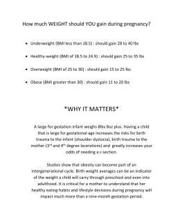


© Copyright 2026