1. No category

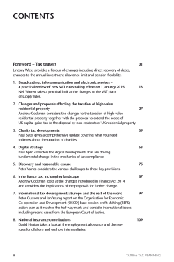
ANNALS OF ECONOMICS AND FINANCE
16-1, 199–229 (2015)
Optimal Income Taxations with Information Asymmetry: The
Lagrange Multiplier Approach
Xiaojun Zhao
School of Economics, Peking University, Beijing, 100871, China
E-mail: [email protected]
This paper considers a general class dynamic optimal problem with incentive compatible constraints. The first-order conditions are derived using the
Lagrange multiplier method. Applied the methods developed here, the optimal
taxation problems studied by Mirrlees (1971) and Golosov et al. (2003) for
more general form utility function are reexamined in this paper. The explicit
solutions for optimal income taxations are derived in this paper. Finally, we
present numerical solutions for optimal income taxations.
Key Words : Incentive compatible constraint; Asymmetric information; Lagrange functional.
JEL Classification Numbers : C61, D90, H00.
1. INTRODUCTION
Many interesting economic problems involve multiple decision makers in
complex environments coupled with information asymmetry. For example,
Mirrlees (1971) assumes asymmetric information in a planner’s economy
and derives the logistical relationship between optimal labor taxation and
labor ability (private information). Rogerson (1985a, 1985b) use a dual
approach to find the first-order optimal conditions in a static principleagent problem. Golosov et al. (2003) and Golosov and Tsyvinski (2006)
use the method developed by Rogerson (1985a, 1985b) to study optimal
indirect taxation in a dynamic environment in which the agent’s skill is
private information and follows arbitrary stochastic processes. Their work
extends Mirrlees’ (1971) famous framework to a dynamic framework and
shows that positive capital taxation is the Pareto optimal choice.
The dual approach developed by Rogerson (1985a, 1985b) should construct a minimized problem that delivers the same utility to all types as
the candidate optimum and satisfies the resource feasibility in all periods.
199
1529-7373/2015
All rights of reproduction in any form reserved.
200
XIAOJUN ZHAO
However, the method cannot be extended directly to a dynamic framework. To apply the dual approach, Golosov et al. (2003) and Golosov
and Tsyvinski (2006) assume that the utility is separable in leisure and
consumption to examine the optimal capital income taxation. Farhi and
Werning (2010) consider the optimal insurance arrangements in a dynamic
Mirrlees economy under the life cycle context. If the utility function is not
separable, then a disturbance in consumption will not only affect the utility from consumption but also the labor supply, which in turn will affect
production. Thus, the dual approach will not work. The separability of
consumption and leisure in the utility function plays an important role in
solving the problem.
On the other hand, Golosov et al. (2003), in contrast, consider only
the optimal capital income tax. Recently, Golosov et al. (2010) consider
the optimal labor taxation in the framework of Golosov et al. (2003).
Applying the Mirrlees envelope theorem (Mirrlees, 1971), they derive the
explicit solution for the optimal labor income taxation under the following
specified utility function
U (c, l) =
1
1
exp[−ψ(c − lγ )],
ψ
γ
where ψ and γ are positive constants. However, Golosov et al. (2010)
cannot depict the optimal taxation rules as the functions of agents’ private
information; they alternatively provide the relationship between the taxation rules and agents’ income. However, Golosov et al. (2010) cannot deal
with the problem with the consideration of both capital and labor income
taxations. This is because the dual approach will not work because a disturbance in consumption will also affect the labor supply when both labor
and capital income taxes are considered.
In fact, Mirrlees (1971), Golosov et al. (2003), and Golosov et al. (2010)
can be also viewed as the extensional framework of optimal dynamic mechanism design, which is consistent with the classical principal-agent framework. Pavan et al. (2009) summarize the first order conditions in more
general optimal dynamic mechanism design problems. He also uses the
Mirrlees envelope theorem to derive the first-order conditions. Garrett and
Pavan (2009) apply the same approach presented in Pavan et al. (2009)
to investigate the optimal incentive scheme for a manager who faces costly
effort decisions and stochastically varying ability over time. They assume
that both the principal and agent are risk-neutral and derive the closed
form solution. This paper focuses mainly on the evolution of the agent’s
ability and demonstrates how the shock affects the compensations of the
manager.
Both the optimal capital and labor income taxations in a uniform framework, and the optimal income taxation under more general utility function
OPTIMAL INCOME TAXATIONS WITH INFORMATION ASYMMETRY 201
are important problems that remain to be solved. These are the main
aims of this paper. We use the Lagrange multiplier method to deal with
a class of more general dynamic optimization problems with asymmetric
information, and use the method developed here to reexamine the optimal
labor income tax and capital income tax in the framework of Golosov et
al. (2003).
The remainder of the paper is organized as follows. In Section 2, we
introduce mathematic results of functional space. In Section 3, we use
the Lagrange multiplier method to deal with general dynamic optimization
problems with private information, in which we apply the truth-telling
constraint. In Section 4, we re-examine optimal income taxation in both
the static and dynamic frameworks. We obtain an optimal income taxation
similar to that of Mirrlees (1971), Golosov et al. (2003), and Golosov and
Tsyvinski (2006). However, we deal with more general forms of the utility
function and with both capital income tax and labor income tax. Section
5 specifies the utility and production functions and presents the numerical
solutions for optimal income taxation. We offer our conclusions in Section
5.
2. SOME MATHEMATICAL RESULTS
In this section, we review useful mathematical results that are important
in the argument that follows.
2.1. Frechet Differentiation
Suppose that (X, k · kX ) and (Y, k · kY ) are two function spaces, and that
N is the set of all linear maps from X to Y . A continuous map Λ ∈ N is
said to be differentiable at point x ∈ X if there exists A ∈ N such that
Λ(x0 ) − Λ(x) = A(x0 − x) + o(kx0 − xkX ), for any x0 ∈ X.
(1)
A is the Frechet differentiation of Λ at x, which we denote as δx∗ Λ. Note
that the Frechet differentiation is an extension of ordinary differentiation
in the Rn space. When Y = R, we call Λ a functional. We state some
important properties of Λ in the following propositions.
Proposition 1. Suppose that Λ : X → R is differentiable on X and
there exists x∗ ∈ U ⊂ X such that Λ(x) ≤ Λ(x∗ ) for all x ∈ U . Then,
δx∗ Λ = 0.
Proof. The proof is easy and we omit it for simplicity.
(2)
202
XIAOJUN ZHAO
Proposition 1 is an extension of the traditional optimization problem in
Rn .
Example 2.1.
If X = C[0, 1] is the set of all continuous functions on
[0, 1] and Λ(x) = f (x(1/2)), then
δx Λ(η) = f 0 (x(1/2))η(1/2)
for all η ∈ X.
Because δx Λ is also a functional, from Proposition 1, δx Λ = 0 means that
f 0 (x(1/2))η(1/2) = 0
for all η ∈ X,
which indicates that f 0 (x(1/2)) = 0.
Example 2.2. Suppose that X is the set
R of all integrable functions in
the probability space (Ω, F, µ), and Λ(x) = f (x)dµ. Then,
Z
δx Λ(η) =
f 0 (x)ηdµ
for all η ∈ X.
Furthermore, δx Λ = 0 means that f 0 (x) = 0.
Definition 2.1.
Λ is a functional on X that is concave if for every
x, y ∈ X and any λ ∈ [0, 1] we have
Λ(λx + (1 − λ)y) ≤ λΛ(x) + (1 − λ)Λ(y).
(3)
Furthermore, Λ is strictly concave on X if for any x 6= y and λ ∈ (0, 1)
Λ(λx + (1 − λ)y) < λΛ(x) + (1 − λ)Λ(y).
(4)
The following proposition connects the Frechet differentiation and this
concavity.
Proposition 2. If Λ is differentiable and concave on X, then for every
x and y ∈ X
Λ(x) − Λ(y) ≥ δx Λ(x − y).
(5)
Proof. The proof is similar to that for X = Rn , and we thus omit it.
OPTIMAL INCOME TAXATIONS WITH INFORMATION ASYMMETRY 203
2.2. The Lagrange Functional
In this section, we consider a discrete-time dynamic optimization problem. First, we define the basic space NT × Ω, where NT = {1, . . . , T } is the
subset of natural numbers and Ω is the sample space. The (Ω, F, µ) is a
probability space with the increasing filtration F = {Ft : t ∈ NT }, F is the
union of all Ft in F, and µ is the measurement on Ω. We define a sequence
of function spaces
Mt = {x : Ω → R, x is bounded and x ∈ Ft }, t ∈ NT ,
(6)
where R is a set of all real numbers. We then define the norm on Mt as
kxk = max |x(ω)|. It follows from Stokey et al. (1989) and Stokey (2009)
ω∈Ω
that (Mt , k.k) is a Banach space.
The dynamic optimization problem is
P1 :
T
X
max E[
β t−1 f (xt , ut )],
xt ,ut ∈Mt
(7)
t=1
subject to
xt+1 = g(xt , ut , εt+1 ),
t = 1, . . . , T − 1,
(8)
with the given initial condition x1 .
Here, xt , ut ∈ Mt are state and control variables, respectively. β ∈ (0, 1)
is the discount factor and εt ∈ Mt is the stochastic disturbance. f and g
are continuous and differentiable functions that are concave with respect
to (x, u).
To solve the optimization problem, we define the Lagrange functional as
" T
# T −1
X
X
t−1
L(x, u, z) = E
β f (xt , ut ) +
hzt+1 , g(xt , ut , εt+1 ) − xt+1 i, (9)
t=1
t=1
where zt ∈ Mt , t = 2, . . . , T is the associated Lagrange multipliers
and h., .i
R
is the inner product, which is defined as hx, yi = E(xy) = xydµ.
This leads to the following proposition.
Proposition 3. If (x∗t , u∗t ), t = 1, . . . , T is a solution for the optimiza-
tion problem (P1), then there exists zt∗ ∈ Mt , t = 2, . . . , T such that
(x∗t , u∗t , zt∗ ) is a local saddle point of the functional L(x, u, z), namely, there
exists ε > 0 such that
L(x∗ , u∗ , z) ≥ L(x∗ , u∗ , z ∗ ) ≥ L(x, u, z ∗ ),
for any x ∈ B(x∗ , ε), u ∈ B(u∗ , ε), and z ∈ B(x∗ , ε).
(10)
204
XIAOJUN ZHAO
The proof is presented in the Appendix.
We can use Frechet differentiations to find the optimal conditions for the
optimization problem (P1). The first-order conditions are δ(x∗ ,u∗ ) L = 0.
The proof is rather easy, and we omit it.
3. DOPS WITH INCENTIVE COMPATIBLE CONSTRAINTS
In this section, we consider a generalized dynamic optimal problem with
incentive compatible constraints. There are two decision makers, A and B.
In examples of this problem, Golosov et al. (2003) consider an economy
with a social planner and agents, and Rogenson (1985a, 1985b) considers
an economy with a principle and an agent. For convenience, we call A
the social planner and B the agent. The social planner allocates economic
resources, and each agent has his or her own private information that is
hidden to the social planner. However, the social planner wants each agent
to report his or her private information. We call this strategy the truthtelling strategy, following the studies of Mirrlees (1971, 1976) and Diamond
and Mirrlees (1986).
3.1. The Basic Settings
Suppose that there is an infinite number of long-lived agents situated
in the real interval [0, 1]. Each agent is indexed by j, j ∈ [0, 1] and has
private information θt in period t. We suppose that θt is independent and
identically distributed (i.i.d) across agents, and that {θt }, t = 1, . . . , T is
defined on a probability space (Ω, F, µ) that is adapted to the increasing
filtration F = {Ft }, t = 1, . . . , T , where F is the union of all of the elements
in F.
In each period, the agent with private information θ is rewarded f (x, u, θ)
through the allocation x, u, where x is the state variable and can be deemed
as the resource and u is the control variable.
As the social planner aims to maximize the sum of rewards for the agents
in the economy, from Uhlig (1996) we obtain
max
j
j
xt ,ut
T
X X
j∈[0,1] t=1
β t−1 f (xjt , ujt , θtj ) = max Eθ [
xt ,ut
T
X
β t−1 f (xt , ut , θt )],
(11)
t=1
where Eθ is the expectation on the random variables θt and β ∈ (0, 1) is
the discount factor.
There are two types of constraints. The first comprises the resource
constraints
xt+1 = g(xt , Λ(ut , θt ));
t = 1, . . . , T − 1,
(12)
OPTIMAL INCOME TAXATIONS WITH INFORMATION ASYMMETRY 205
where Λ(ut , θt ) = (Λ1 (ut , θt ), . . . , Λm (ut , θt )) is a functional of the random
variables ut and θt and is defined as the aggregate effect of private information and resource allocations on resource accumulation.
The other type of constraint for the social planner is the incentive compatible constraint (IC). Suppose that the social planner wants the agent
to report his or her private information to enable the allocation of social
T
resources. A report strategy is defined as maps σ : ΘT → Θ , and the set
of all report strategies is denoted by Σ. Under report strategy σ, we denote
the discounted gains for the agent with private information θ ∈ ΘT as
W (σ, θ) =
T
X
β t−1 f (xt (σ(θ)), ut (σ(θ)), θt ).
(13)
t=1
σ ∗ is a truth-telling strategy if σ ∗ (θ) = θ for all θ. Thus, an allocation is
incentive compatible (IC) if
W (σ ∗ , θ) ≥ W (σ, θ)
for any
θ ∈ ΘT , σ ∈ Σ.
(14)
The dynamic optimization problem with IC constraints can then be summarized as
" T
#
X
t−1
P2: max Eθ
β f (xt , ut , θt ) ,
xt ,ut
t=1
subject to the resource constraints (12) and the IC constraints (14) with
the given initial condition x1 .
In the next subsection, we use the Lagrange method to solve the optimization problem (P2). For simplification, we assume that xt ∈ R and
ut ∈ Rn .
3.2. Optimal Conditions
In this section, we use the Lagrange method to find the optimal conditions for the dynamic optimization problem (P2). First, the IC constraint
(14) can be rewritten as
T
X
β t−1 f (xt (θ0 ), ut (θ0 ), θt ) ≤
t=1
T
X
β t−1 f (xt (θ), ut (θ), θt ),
(15)
t=1
for any θ ∈ ΘT and θ0 ∈ ΘT .
To solve the optimization problem, we define the Lagrange functional
L(x, u) = Eθ [
T
X
β t−1 f (xt , ut , θt )] +
t=1
+ Eθ0 ,θ λ(θ0 , θ)
T
X
β t−1 λt (g(xt , Λ(ut , θt )) − xt+1 )
t=1
T
X
t=1
β t−1 (f (xt (θ), ut (θ), θt ) − f (xt (θ0 ), ut (θ0 ), θt )),
(16)
206
XIAOJUN ZHAO
where λ(θ0 , θ) : ΘT × ΘT −→ R are the Lagrange multipliers1 for the IC
constraint (15) and λt , t = 1, 2, . . . , T are the Lagrange multipliers for the
resource constraints (12). It is easy to find that λ(θ0 , θ) is measurable on
F × F, and that λt is a non-stochastic number.
This leads to the following proposition.
Proposition 4. The optimal conditions for the optimization problem
P2 are
λt = βλt+1 gx (xt+1 (θ), Λ(ut+1 (θ), θt+1 ))
+ βE[(1 + Eθ0 λ(θ0 , θ))fx (xt+1 (θ), ut+1 (θ), θt+1 )]
0
− βE λ(θ, θ0 )fx (xt+1 (θ), ut+1 (θ), θt+1
)
(17)
and
λt
m
X
gΛj (xt , Λ(ut , θt ))δui Λj (ut , θt )
j=1
= −(1 + Et [Eθ0 λ(θ0 , θ)])fui (xt (θ), ut (θ), θt )
+ Et [Eθ0 [λ(θ, θ0 )fui (xt (θ), ut (θ), θt0 )]] ,
(18)
where δui Λj is the Rize reprentative of the Frechet differentiation of Λj
with respect to ui at t.
Proof. The Lagrange functional (16) can be rewritten as
L(x, u) =
T
X
β t−1 [(1 + Eθ0 [λ(θ0 , θ)])f (xt (θ), ut (θ), θt )]
t=1
−
T
X
β t−1 Eθ0 [λ(θ, θ0 )f (xt (θ), ut (θ), θt0 )]
t=1
+
T
X
β t−1 λt (g(xt , Λ(ut , θt )) − xt+1 ).
t=1
We then obtain the optimialities by taking the Frechet differentiations
of L with respect to xt and uit , i = 1, . . . , n.
hλt − βλt+1 gx (xt+1 , Λ(ut+1 , θt+1 )), ηi
= hβ(1 + Eθ0 [λ(θ0 , θ)])fx (xt+1 (θ), ut+1 (θ), θt+1 ), ηi
0
− hβEθ0 λ(θ, θ0 )fx (xt+1 (θ), ut+1 (θ), θt+1
) , ηi
1 Here,
λ(θ0 , θ) means that an agent has private information θ but reports θ0 .
(19)
OPTIMAL INCOME TAXATIONS WITH INFORMATION ASYMMETRY 207
h(1 + Eθ0 [λ(θ0 , θ)])fui (xt (θ), ut (θ), θt ) − Eθ0 [λ(θ, θ0 )fui (xt (θ), ut (θ), θt0 )]
m
X
+ λt
(20)
gΛj (xt , Λ(ut , θt ))δui Λj (ut , θt ), ξi = 0
j=1
for all ξ ∈ Ft and η ∈ R.
From equations (19) and (20), it is easy to see that equations (17) and
(18) hold.
Proposition 4 can be used to deal with more general dynamic optimization problems with incentive compatible constraints. From equations (17)
and (18), we can derive the “inverse Euler equation” similar to Golosov
et al. (2003) and many other existing literatures. To understand these
conditions more intuitional, we define
0
e θt ) = 1 + Eθ0 [λ(θ0 , θ) − λ(θ, θ0 ) fx (xt (θ), ut (θ), θt ) ],
λ(θ,
fx (xt (θ), ut (θ), θt )
and
µi (θ, θt ) = 1 + Eθ0 [λ(θ0 , θ) − λ(θ, θ0 )
fui (xt (θ), ut (θ), θt0 )
].
fui (xt (θ), ut (θ), θt )
Then, equations (17) and (18) can be rewritten as
e θt+1 )fx (xt+1 (θ), ut+1 (θ), θt+1 )],
λt = β [λt+1 gx (xt+1 (θ), Λ(ut+1 (θ), θt+1 ))]+βE[λ(θ,
and
λt
m
X
gΛj (xt (θ), Λ(ut (θ), θt ))δui Λj (ut (θ), θt ) = −Et [µi (θ, θt )] fui (xt (θ), ut (θ), θt ).
j=1
Furthermore, we define
fui (xt (θ), ut (θ), θt )
,
g
(x
(θ),
Λ(ut (θ), θt ))δui Λj (ut (θ), θt )
t
j=1 Λj
ϕi (t) = Pm
and
ψi (t) = gx (xt (θ), Λ(ut (θ), θt ))
m
X
e θt )]
fx (xt (θ), ut (θ), θt )Et [λ(θ,
.
−
gΛj (xt (θ), Λ(ut (θ), θt ))δui Λj (ut (θ), θt )
fui (xt (θ), ut (θ), θt )Et [µi (θ, θt )]
j=1
208
XIAOJUN ZHAO
Therefore, we have
λt = β [λt+1 Eψi (t + 1)] ,
(21)
λt = −Et [µi (θ, θt )] ϕi (t).
(22)
and
From equations (21) and (22), we can derive a generalized inverse Euler
equation similar to that in Golosov et al. (2003) and Golosov and Tsyvinski (2006). However, the method developed here is more general, and can
be deal woth more general dynamic problems with asymmetric information. In the next section, we will apply this method to study the optimal
income taxations in an general economic system with incentive compatible
constraints.
4. THE OPTIMAL INCOME TAXATIONS
In public finance and macroeconomics research, attempts to incorporate
information asymmetry into economic models to study the optimal fiscal
policy begin with Mirrlees (1971). He derives the optimal labor income
tax and asserts the logistic relationship between the optimal labor income
tax rate and the agent’s ability (private information). His seminal findings
have encouraged many scholars to step into this area. Golosov et al. (2003)
extend Mirrlees’ (1971) static framework to a dynamic framework to analyze the optimal capital income tax. Golosov et al. (2003) do not consider
the optimal labor income tax, and we cannot compare the optimal labor
income tax in the static and dynamic frameworks. In this section, we apply
the Lagrange method to re-examine Mirrlees’ (1971) optimal labor income
tax in a static environment and the Golosov et al. (2003) optimal income
taxes (capital income tax and labor income tax) in a dynamic environment.
4.1. The Static Mirrlees Model
The framework of the static Mirrlees model is simple. The agent’s labor ability θ is a random variable on the measurable space (Ω, F, µ), and
the range of θ is Θ. Thus, an agent’s effective labor supply l is l × θ,
which we denote as y. The agent’s utility function is defined by his or her
consumption c and the labor supply l, which mathematically is U (c, y/θ).
4.1.1.
Social planner’s economy
Suppose that the production function is H(Y ), where Y =
the aggregate effective labor supply in the economy.
R
y(θ)dµ is
OPTIMAL INCOME TAXATIONS WITH INFORMATION ASYMMETRY 209
The optimal allocation problem for the social planner is
Z
U (c(θ), y(θ)/θ)dµ
max
(23)
c(θ),y(θ)
subject to the resource constraint
Z
Z
c(θ)dµ = H( y(θ)dµ),
(24)
and IC constraints
U (c(θ), y(θ)/θ) ≥ U (c(θ0 ), y(θ0 )/θ), for any θ, θ0 ∈ Θ.
(25)
From equations (17) and (18), the optimal conditions for this optimization problem can be easily obtained as
λ = (1 + Eθ0 λ(θ0 , θ))Uc (c(θ), y(θ)/θ) − Eθ0 [λ(θ, θ0 )Uc (c(θ), y(θ)/θ0 )] , (26)
and
−λH 0 (Y ) = (1 + Eθ0 λ(θ0 , θ))Ul (c(θ), y(θ)/θ)/θ
−Eθ0 [λ(θ, θ0 )Ul (c(θ), y(θ)/θ0 )/θ0 ] ,
(27)
where λ is the Lagrange multiplier for the resource constraint (24) and
λ(θ0 , θ) is the Lagrange multipliers for the IC constraints (25).
To obtain some interesting results, we place further restrictions on U (c, l).
Case 1. U (c(θ), y(θ)/θ0 ) = u(c(θ), y(θ)/θ)v(θ, θ0 ) with v(θ, θ) = 1.
In this case, we let λ(θ) = 1 + Eθ0 [λ(θ0 , θ)(1 − v(θ, θ0 ))], which means
that equations (26) and (27) become
λ = λ(θ)uc (c(θ), y(θ)/θ) and − λH 0 (Y ) = λ(θ)ul (c(θ), y(θ)/θ)/θ.
This gives
−ul (c(θ), y(θ)/θ)/θ = uc (c(θ), y(θ)/θ)H 0 (Y ).
(28)
Case 2. U (c(θ), y(θ)/θ0 ) = u(c(θ)) − v(y(θ)/θ)w(θ, θ0 ) with w(θ, θ) = 1.
In this case, equations (26) and (27) become
λ = (1 + Eθ0 (λ(θ0 , θ) − Eθ0 λ(θ, θ0 ))u0 (c(θ)),
and
λH 0 (Y ) = (1 + Eθ0 λ(θ0 , θ) − Eθ0 [λ(θ, θ0 )w(θ, θ0 )])v 0 (y(θ)/θ)/θ.
210
XIAOJUN ZHAO
This gives
v 0 (y(θ)/θ)/θ =
1 + Eθ0 [λ(θ0 , θ) − λ(θ, θ0 )]
u0 (c(θ))H 0 (Y ).
1 + Eθ0 [λ(θ0 , θ) − λ(θ, θ0 )w(θ, θ0 )]
(28)
Equation (29) is the same as the optimal conditions in Mirrlees (1971) with
the the separable utility function.
Case 3. U (c(θ), y(θ)/θ0 ) = u(c(θ))v(y(θ)/θ0 ).
In this case, we let
v(y/θ0 )
λ(θ, y) = 1 + Eθ0 λ(θ0 , θ) − λ(θ, θ0 )
v(y/θ)
and
0
0
0
0 v (y/θ )θ
.
µ(θ, y) = 1 + E λ(θ , θ) − λ(θ, θ ) 0
v (y/θ)θ0
θ0
The optimal conditions (26) and (27) can be deduced to
v 0 (y(θ)/θ)/θ
λ(θ, y) u0 (c(θ)) 0
=
H (Y ).
v(y(θ)/θ)
µ(θ, y) u(c(θ))
(29)
Equations (28), (29), and (30) determine the optimal conditions under
the three specified utility function, we will use them to derive the optimal
labor income taxation accordingly.
4.1.2.
Decentralized economy
To derive the implementation mechanism, we consider a decentralized
economy. Suppose that there is a representative firm in the economy and
that agents work in it to earn income. The government levies a labor
income tax in its budget.
Agents.
An agent with ability θ aims to maximize his/her utility under the budget
constraint, that is,
max U (c(θ), y(θ)/θ)
c,y
subject to the budget constraint
c(θ) = (1 − τ w )ωy(θ) + χ(θ),
(30)
where ω is the wage rate, τ w is the labor incoem tax rate, and χ(θ) is
government’s transfer.
OPTIMAL INCOME TAXATIONS WITH INFORMATION ASYMMETRY 211
It is easy to derive the optimal condition
−Ul (c(θ), y(θ)/θ)/θ = (1 − τ w )ωUc (c(θ), y(θ)/θ).
(31)
Firms.
The firm’s profit maximization π = maxY H(Y ) − ωY indicates that
ω = H 0 (Y ).
(32)
Government.
Under the balance budget constraint, government’s transfer equals the
tax revenue, namely,
Z
Z
χ(θ)dµ = τ w ωy(θ)dµ + π.
(33)
Macroeconomic equilibrium.
Combining equations (31), (32), (33), and (34), we obtain the optimal
conditions in the macroeconomic equlibrium
−Ul (c(θ), y(θ)/θ)/θ = (1 − τ w )H 0 (Y )Uc (c(θ), y(θ)/θ),
(34)
and
Z
Z
c(θ)dµ = H(
y(θ)dµ).
(35)
Equations (35) and (36) can be used to derive the optimal labor income
taxation.
4.1.3.
Optimal taxations
In this subsection, we will derive the optimal taxations by setting the
tax policy in the decentralizaed economy implement the social optimum.
We will consider three cases respectively.
In case 1. Equation (35) is compared to equation (28) to give an optimal
labor income tax rate of zero.
In case 2. Equation (35) is compared to equation (29) to give an optimal
labor income rate of
τ w (θ) =
Eθ0 [λ(θ, θ0 )(1 − w(θ, θ0 ))]
,
1 + Eθ0 [λ(θ0 , θ)(1 − w(θ, θ0 ))]
which is dependent on agent’s labor ability θ.
(36)
212
XIAOJUN ZHAO
In case 3. Under the specified utlity form in this case, the optimal
condition (35) can be rewritten as
v 0 (y(θ)/θ)/θ
u0 (c(θ)) 0
= (1 − τ w )
H (Y ).
v(y(θ)/θ)
u(c(θ))
Comparing the above equation with equation (30), the optimal labor
income tax rate can be easily obtained as
v 0 (y/θ 0 )θ
v 0 (y/θ)θ 0 )]
0 (y/θ 0 )θ .
λ(θ, θ0 ) vv0 (y/θ)θ
0]
0
τ
w
=
)
Eθ0 [λ(θ, θ0 )( v(y/θ
v(y/θ) −
1 + Eθ0 [λ(θ0 , θ) −
(37)
Remark 4.1. Under the specified utility function in case 1, the optimal
labor income tax rate is zero, which is the same as in many studies, such
as those of, Chamley (1986) and Judd (1985) etc. Many familiar utility
functions satisfy assumption in case 1. For example, suppose that
U (c, l) =
(cω l−ε )1−σ
,
1−σ
where ω, ε, and σ > 0 are constants. Then,
U (c, y(θ)/θ0 ) =
(cω (y(θ)/θ0 )−ε )1−σ
(cω (y(θ)/θ)−ε )1−σ
=
(θ/θ0 )−ε(1−σ) .
1−σ
1−σ
It is easy to find that the optimal labor income tax is zero with this utility
function.
Remark 4.2. Under the separable utility in case 2, equation (38) gives
the optimal labor income tax rate, which is similar to that of Mirrlees
(1971). For example, suppose that the utility function
U (c, l) = u(c) − lα ,
for 0 < α < 1. Then,
U (c, y(θ)/θ0 ) = u(c) − (y(θ)/θ)α (θ/θ0 )α ,
and w(θ, θ0 ) = (θ/θ0 )α .
Thus, for the agent with the greatest ability, where θ ≥ θ0 , we have
w
τ (θ) ≤ 0, and for the agent with the least ability we have τ w (θ) ≥ 0. We
can also use numerical simulation to find the logistic relationship between
OPTIMAL INCOME TAXATIONS WITH INFORMATION ASYMMETRY 213
the labor income tax rate and the agent’s ability, but for simplicity we omit
this discussion and instead consider the dynamic Mirrlees model.
Remark 4.3. Case 3 presents the optimal labor income tax for more
general utility funtions, for example, similar to Golosov et al. (2010),
U (c, l) = −
1
1
exp[−ψ(c − lγ )],
ψ
γ
where γ and ψ are positive constant.
4.2.
The Dynamic Mirrlees Model
In this section, we re-examine the model introduced in Golosov et al.
(2003) and give its explicit solution. Golosov et al. (2003) consider an
environment in which an agent’s skill is private information. Following
Golosov et al. (2003), we define an agent’s utility by his or her consumption ct and the amount of time spent working in period t by lt , which
mathematically is U (ct , lt ). We assume that θt is the agent’s skill vector in
period t and that both θt and lt are private information of the agent. We
present the framework briefly in the following. More details can be found
in the Golosov et al. (2003).
4.2.1.
Decentralized economy
The foregoing sections tell the story for a planner’s economy. In this
section, we implement the optimal allocation from the planner’s economy
in a decentralized economy, following the framework of Chamley (1986).
Agents.
Suppose that the government levies a capital income tax and a labor
income tax, denoted as τtk and τtw , respectively. Further, suppose that an
agent at time t only knows his or her own ability θt , but does not know his
or her ability θs for all s > t. The agent thus faces future uncertainty, and
must determine the consumption and labor supply by solving the following
problem
∞
X
max E[
β t−1 U (ct , yt /θt )],
ct ,yt
(38)
t=1
subject to
At+1 = (1 − τtk )rt At + (1 − τtw )wt yt − ct + χt ,
(39)
214
XIAOJUN ZHAO
with the given initial asset A0 .
Here, At is the agent’s asset at time t, rt and wt are the market interest
rate and wage rate, respectively, and χt is the government’s transfer.
The first-order conditions can be easily derived as
k
Uc (ct , yt /θt ) = βEt {(1 − τt+1
)rt+1 Uc (ct+1 , yt+1 /θt+1 )},
(40)
(1 − τtw )wt Uc (ct , yt /θt ) = −Ul (ct , yt /θt )/θt ,
(41)
and
where Uc and Ul are the partial differentiations of consumption c and labor
l = y/θ, respectively.
Firms.
Suppose that output is produced by firms with capital and efficient labor
input. The production function is thus neoclassical. The profit maximization problem for firms is then
Z
max f (kt ,
kt ,yt
Z
yt dµ) − rt kt − wt
yt dµ + (1 − δ)kt ,
R
where kt and yt dµ are the aggregate capital and aggregate labor force,
respectively, and δ is the rate of depreciation of capital.
The first-order conditions are
Z
Z
rt = fk (kt , yt dµ) + 1 − δ,
wt = fy (kt , yt dµ),
(42)
R
whereRfy (kt , yt dµ) is the partial differentiation of the aggergate effective
labor yt dµ at time t.
Equilibrium.
R
R
In macro-equilibrium, kt = At dµ and χt dµ = 0, and we thus have
kt+1 = (1 − τtk )rt kt + (1 − τtw )wt
Z
Z
yt dµ −
ct dµ.
(43)
This is just the resource constraint of the economy.
Substituting equation (43) into equations (41) and (42), we arrive at
Uc (ct , yt /θt ) =
k
βEt {(1−τt+1
)
Z
fk (kt+1 , yt+1 dµ) + 1 − δ Uc (ct+1 , yt+1 /θt+1 )},
(44)
OPTIMAL INCOME TAXATIONS WITH INFORMATION ASYMMETRY 215
and
(1 − τtw )fy (kt ,
Z
yt dµ)Uc (ct , yt /θt ) = −
Ul (ct , yt /θt )
.
θt
(45)
The dynamics for a competition economy are thus described by equations
(44), (45), and (46).
4.2.2.
Social planner’s economy
Similar to Golosov et al. (2003), the social planner can observe the
effective labor yt = lt θt for the agent and use the truth-telling mechanism
to obtain private information. The social planner maximizes the social
welfare subject to the social resource constraints and incentive compatible
constraints. This gives the following dynamic optimization problem.
∞
X
max Eθ [
β t−1 U (ct , yt /θt )],
ct ,yt
(46)
t=1
subject to
Z
Z
yt dµ) −
kt+1 = f (kt ,
ct dµ + (1 − δ)kt ,
(47)
and
W (σ ∗ , θ) ≥ W (σ, θ),
(48)
with the given initial condition k1 , where W (σ, θ) is defined as
∞
X
W (σ, θ) = Eθ [
β t−1 U (ct (σ(θt )), yt (σ(θt ))/θt )].
t=1
Similar to equations (17) and (18), the optimal conditions can be easily
derived as
λt = βλt+1 Rt+1 ,
(49)
λt = Et [(1 + Eθ0 λ(θ0 , θ))] Uc (ct (θ), yt (θ)/θt )
− Et [Eθ0 [λ(θ, θ0 )Uc (ct (θ), yt (θ)/θt0 )]] ,
(50)
and
Z
−λt fy (kt ,
yt dµ) = Et [1 + Eθ0 λ(θ0 , θ)] Ul (ct (θ), yt (θ)/θt )/θt
− Et [Eθ0 [λ(θ, θ0 )Ul (ct (θ), yt (θ)/θt0 )/θt0 ]] ,
(51)
216
XIAOJUN ZHAO
R
where Rt = fk (kt , yt dµ) + 1 − δ.
Equations (50), (51), and (52) determine the competitive equilibrium.
Similar to the static Mirrlees economy, we specify the following cases.
Case 1. U (c(θ), y(θ)/θ0 ) = u(c(θ), y(θ)/θ)v(θ, θ0 ) with v(θ, θ) = 1.
e t , θ0 ) = 1 + Eθ0 [λ(θ0 , θ) −
We denote λ(θ) = Eθ0 [λ(θ0 , θ) − λ(θ, θ0 )] and λ(θ
t
0
0
λ(θ, θ )v(θt , θt )]. Equations (50), (51), and (52) then become
λt = βλt+1 Rt+1 ,
(52)
λt = Et [λ(θ)] uc (ct (θ), yt (θ)/θt ),
(53)
and
Z
−λt fy (kt ,
yt dµ) = Et [λ(θ)] ul (ct (θ), yt (θ)/θt )/θt .
(54)
Note that λt ∈ R, and we thus obtain
uc (ct (θ), yt (θ)/θt ) = βRt+1
1
,
Et [1/uc (ct+1 (θ), yt+1 (θ)/θt+1 )]
(55)
and
Z
−ul (ct (θ), yt (θ)/θt )/θt = fy (kt ,
yt dµ)uc (ct (θ), yt (θ)/θt ).
(56)
Equation (56) is an inverse Euler equation that is the same as used by
Golosov et al. (2003). Comparing equations (45) and (46) with equations
(56) and (57) gives
τtw = 0
(57)
and
k
Et (1 − τt+1
)Rt+1 uc (ct+1 (θ), yt+1 (θ)/θt+1 ) = Rt+1
1
.
Et [1/uc (ct+1 (θ), yt+1 (θ)/θt+1 )]
Thus,
1
uc (ct+1 (θ), yt+1 (θ)/θt+1 )Et [1/uc (ct+1 (θ), yt+1 (θ)/θt+1 )]
+
,
(58)
uc (ct+1 (θ), yt+1 (θ)/θt+1 )
k
τt+1
= 1−
where satisfies Et [] = 0.
OPTIMAL INCOME TAXATIONS WITH INFORMATION ASYMMETRY 217
k
k
If τt+1
∈ Ft , then τt+1
has the unique solution
k
τt+1
=1−
1
.
Et [uc (ct+1 (θ), yt+1 (θ)/θt+1 )] Et [1/uc (ct+1 (θ), yt+1 (θ)/θt+1 )]
(59)
Remark 4.4. Equation (58) indicates that the optimal labor income tax
rate is zero under case 1, which is similar to the static case previously stated.
Equation (59) presents the optimal capital income tax rate, which states
that many tax policies can be applied to implement the social optimum.
This conclusion can be compared with that of Zhu (1992), who studies
optimal taxation in an economy with production shocks.
k
Furthermore, if τt+1
∈ Ft , then we derive the same optimal capital income tax rate as Golosov et al. (2003). Similarly, because
1−
1
> 0,
Et [uc (ct+1 (θ), yt+1 (θ)/θt+1 )] Et [1/uc (ct+1 (θ), yt+1 (θ)/θt+1 )]
k
we know that τt+1
> 0. However, the utility form used here is nonseparable.
Case 2. U (c(θ), y(θ)/θ0 ) = u(c(θ)) − v(y(θ)/θ)w(θ, θ0 ) with w(θ, θ) = 1.
This case is similar to that of Golosov et al. (2003), except that the
e θ0 ) = 1 + Eθ0 [λ(θ0 , θ) − λ(θ, θ0 )w(θt , θ0 )] and
utility is separable. We let λ(θ,
t
define λ(θ) as that of case 1, the optimal conditions are then
u0 (ct (θ)) = βRt+1
1
,
Et [1/u0 (ct+1 (θ))]
(60)
and
v 0 (y(θt )/θt )/θt =
Et [λ(θ)]
F (k ,
e θt )] y t
Et [λ(θ,
Z
yt dµ)u0 (ct (θ)).
(61)
Comparing equations (45) and (46) with equations (61) and (62) gives
k
τt+1
=1−
1
,
Et [u0 (ct+1 (θ))] Et [1/u0 (ct+1 (θ))]
(62)
and
τtw =
Et {Eθ0 [λ(θ, θ0 )(1 − w(θt , θt0 ))]}
.
1 + Et {Eθ0 [λ(θ0 , θ)] − Eθ0 [λ(θ, θ0 )w(θt , θt0 )]}
(63)
Remark 4.5. With the same function as that of Golosov et al. (2003),
equation (63) states the same optimal capital income tax. However, equa-
218
XIAOJUN ZHAO
tion (64) presents the same optimal labor income tax rate as that of Mirrlees
(1971).
For these two cases, we derive the same capital income tax rate but
different optimal labor income tax rates. Under the non-separable utility
function, the disturbance of consumption and labor supply not only affect
the resource constraint, but also the IC constraints.
Case 3. U (c(θ), y(θ)/θ0 ) = u(c(θ))v(y(θ)/θ0 ).
In this case, the first-order conditions (45) and (46) for the decentralized
economy can be reduced as:
k
u0 (c(θt ))v(y(θt )/θt ) = β(1 − τt+1
)Rt+1 Et [u0 (c(θt+1 ))v(y(θt+1 )/θt+1 )],
(64)
and
Z
u(c(θt ))v 0 (y(θt )/θt )
. (65)
(1 − τtw )Fy (kt , yt dµ)u0 (c(θt ))v(y(θt )/θt ) = −
θt
As for the social planner economy, let
0
e yt , θ0 ) = 1 + Eθ0 [λ(θ0 , θ) − λ(θ, θ0 ) v(yt /θt ) ],
λ(θ,
t
v(yt /θt )
and
µ(θ, yt , θt0 ) = 1 + Eθ0 [λ(θ0 , θ) − λ(θ, θ0 )
v 0 (yt /θt0 )θt
].
v 0 (yt /θt )θt0
Then, we can rewrite equations (50), (51), and (52) as
λt = βλt+1 Rt+1 ,
e yt , θ0 )]u0 (c(θt ))v(y(θt )/θt ),
λt = Et [λ(θ,
t
and
Z
−λt Fy (kt ,
yt dµ) = Et [µ(θ, yt , θt0 )] u(c(θt ))v 0 (y(θt )/θt )/θt .
Therefore, we further have
u0 (c(θt ))v(y(θt )/θt ) = βRt+1
Et
[1/u0 (c(θ
1
,
t+1 ))v(y(θt+1 )/θt+1 )]
(66)
OPTIMAL INCOME TAXATIONS WITH INFORMATION ASYMMETRY 219
and
Z
e yt , θ0 )]
Et [λ(θ,
u(c(θt ))v 0 (y(θt )/θt )
t
0
F
(k
,
y
dµ)u
.
(c(θ
))v(y(θ
)/θ
)
=
−
y
t
t
t
t
t
Et [µ(θ, yt , θt0 )]
θt
(67)
Equation (67) restates the “Inverse Euler Equation” as that in Golosov
et al. (2003) and many existing literatures. Comparing it with (65) and
k
assuming τt+1
∈ Ft , then
1
.
Et [uc (ct+1 (θ), yt+1 (θ)/θt+1 )] Et [1/uc (ct+1 (θ), yt+1 (θ)/θt+1 )]
(68)
Similarly, comparing equation (68) with equation (66), we have
k
τt+1
=1−
v 0 (yt /θt0 )θt
v 0 (yt /θt )θt0 )]}
.
v 0 (y /θ 0 )θ
Eθ0 [λ(θ, θ0 ) v0 (ytt /θtt )θt0 ]}
t
v(y /θ 0 )
τtw =
Et {Eθ0 [λ(θ, θ0 )( v(ytt /θtt ) −
1 + Et {Eθ0 [λ(θ0 , θ)] −
(69)
Remark 4.6. Equations (70) gives the similar optimal labor income
taxation to Golosov et al. (2010), where he specifies the utility function as
U (c, l) = −
1
1
exp[−ψ(c − lγ )].
ψ
γ
In fact, we can rewrite this utility function as
U (c, l) = −
1
exp(−ψc) exp(ψlγ /γ),
ψ
which is just the same forms as Case 3 here.
Furthermore, we not only give the optimal labor income taxation but also
the optimal capital income taxation. Using the dual approach developed
by Rogerson (1985), we cannot deal with both the capital and labor income
taxations. So in case 3, we have included the case in Golosov et al. (2010)
and provide all income taxation by applying the Lagrange multiplier.
5. NUMERICAL RESULTS
In this section, we use the second-order approximation method presented
by Schmitt-Grohe and Uribe (2004) to simulate the mentioned static and
dynamic Mirrlees models. First, we give the optimal labor income taxation
in both the static and dynamic Mirrlees models. We also present the optimal capital income taxation in the dynamic Mirrlees model. Second, we
220
XIAOJUN ZHAO
provide comparative static results and give the effects of some important
parameters on the optimal taxation rules. Finally, we calculate the tax
burdens for different population groups.
To simulate the model, we specify the utility function as
u(c, l) =
c1−σ − 1
− lγ ,
1−σ
(70)
where σ > 0 and γ > 0 are positive constants.
In the static Mirrless model, we specify the production function as H(y) =
y α , where 0 < α < 1 is a constant. For the dynamic Mirrlees model, we
specify the production function as f (k, l) = k α l1−α .
We assume that the stochastic process {θt } is uniformly distributed on
the interval [2, 22]. To make the simulation results more convincing, we
identify the common parameters in the model as T = 30 being the periods
for which the economy lasts, the discountor for utility, β = 0.9, and γ = 2.
To allow comparison, we set the parameters σ = 2 and σ = 3, α = 0.3,
and α = 0.6. We set the representative time as t = 5, t = 10, t = 15, and
t = 20 to test the trends of the policies as times go.
Figure 1 presents the optimal labor income taxation in the static Mirrlees
model.
FIG. 1. The Optimal Labor Income Tax in the Static Mirrlees Model
Labor Income Taxations
18
16
14
12
10
y
Tt
8
6
4
2
0
2
4
6
8
10
12
θt
14
16
18
20
22
Figure 1 depicts the relationship between labor income taxation and
labor ability in the static Mirrlees (1971) model; the corresponding parameters are set as σ = 2, γ = 0.5, and α = 0.7. The logistic curve states that
the optimal taxation rules are to give agents incentives in two ways. The
marginal tax of a person with labor ability θ ≥ 16 will decrease as their
labor ability increases, which will give the person the incentive to provide
OPTIMAL INCOME TAXATIONS WITH INFORMATION ASYMMETRY 221
more effective labor. The marginal tax of the rest of people will increase
as their labor ability increases. Agents with medium labor ability pay the
highest marginal tax.
In the case of the dynamic Mirrlees model, we suppose that the government’s transfer policy is set to equalize each person in society. The
associated capital income tax Ttk = τtk rt k, is indeed a function of τtk . Figures 2 and 3 state the optimal capital and labor income tax rates via the
agent’s labor ability, respectively.
FIG. 2. The Optimal Capital Income Tax in the Dynamic Mirrlees Model
Capital Taxation Rates in Dynamic Economics
0.4
0.35
0.3
0.25
τk
t
0.2
0.15
0.1
0.05
0
2
4
6
8
10
12
θt
14
16
18
20
22
FIG. 3. The Optimal Labor Income Tax in the Dynamic Mirrlees Model
Labor Income Taxation in Dynamic Economics
30
25
20
y
Tt
15
10
5
0
2
4
6
8
10
12
θt
14
16
18
20
22
Similar to the previous discussion, both the optimal labor income tax
and capital income tax are positive. Furthermore, Figure 2 shows that the
optimal capital income tax rate is a decreasing function of the agent’s labor
ability. Similar to Figure 1 in the static Mirrlees model, Figure 3 also states
222
XIAOJUN ZHAO
a logistic relationship between the optimal labor income tax rate and the
agent’s labor ability.
The reason for the negative relationship between the government’s capital income tax and the agent’s labor ability is that the government should
give agents with higher labor ability the incentive to accumulate more.
The logistic relationship between the optimal labor income tax rate and
the agent’s labor ability can be explained in line with Mirrlees (1971) as
that, the government should give agents with higher labor ability the incentive to work more, because the marginal labor income tax decreases with
the agents’ labor ability.
5.1.
Comparative Static Results
In this subsection, we report the effects of certain parameters on the
optimal taxations. For simplicity, we consider two parameters, relative
risk aversion σ and capital/output ratio α, and inspect their effects on the
optimal taxation rules. We set σ = 2, σ = 3, and α = 0.3, α = 0.6 for the
experiment.
5.1.1.
Optimal capital income taxation via σ and α
Figures 4 and 5 present the effects of relative risk aversion σ and capital/output ratio α on the optimal capital income taxation.
FIG. 4. The Effects of σ to the Capital Income Tax
σ=2
σ=3
0.4
0.7
0.35
0.6
0.3
0.5
0.25
τk
t
τk
0.4
t
0.2
0.3
0.15
0.2
0.1
0.1
0.05
0
2
4
6
8
10
12
θt
14
16
18
20
22
0
2
4
6
8
10
12
θt
14
16
18
20
22
Figure 4 depicts that the curves of the labor ability and capital income
tax become convex to the origin as the coefficient of the relative risk aversion σ increases. Because we set the time t = 10, the two subfigures are
decreasing curves. Note that the curve with σ = 3 lies above that with
σ = 2, which shows that as the relative risk aversion increases, the tax
burden will increase. The effects of capital/output ratio α on the optimal
capital income tax is similar to the effects of σ, which are depicted in Figure
5.
OPTIMAL INCOME TAXATIONS WITH INFORMATION ASYMMETRY 223
FIG. 5. The Effects of α to the Capital Income Tax
α=0.3
α=0.5
0.45
0.7
0.4
0.6
0.35
0.5
0.3
τkt
0.25
τkt
0.2
0.4
0.3
0.15
0.2
0.1
0.1
0.05
0
5.1.2.
2
4
6
8
10
12
θt
14
16
18
20
0
22
2
4
6
8
10
12
θt
14
16
18
20
22
Optimal labor income taxation via σ and α
The following figures consider the effects of parameters σ and α on the
optimal labor income taxation.
FIG. 6. The Effects of σ to the Labor Income Tax
σ=2
σ=3
0.35
0.35
0.3
0.3
0.25
0.25
0.2
0.2
Ty
Ty
t
t
0.15
0.15
0.1
0.1
0.05
0.05
0
2
4
6
8
10
12
θt
14
16
18
20
0
22
2
4
6
8
10
12
θt
14
16
18
20
22
20
22
FIG. 7. The Effects of α to the Labor Income Tax
α=0.3
α=0.5
0.25
0.25
0.2
0.2
0.15
0.15
Tty
Tty
0.1
0.1
0.05
0.05
0
2
4
6
8
10
12
θt
14
16
18
20
22
0
2
4
6
8
10
12
θt
14
16
18
224
XIAOJUN ZHAO
Figure 6 illustrates the effects of the coefficient of relative risk aversion
σ. The logistic curve become flatter as σ increases, and the tax increases
at the same time. With σ increasing, the agents care more about their consumption and thus the decreasing marginal labor income tax for the agent
with medium labor ability raises that actor’s confidence about consumption. Hence, the curve becomes more flat. With the same reasoning, we
also report the effects of capital/output ratio α in Figure 7. As α increases,
the labor income decreases relatively, which in turn decreases the marginal
labor income tax for the agent with medium labor ability and the logistic
curve again appears to be flatter.
5.2.
The Distribution of the Tax Burden
In this subsection, we investigate the tax burden for different groups of
the population. Letting t = 10 and πt be the ratio of the tax burden for
the agent with labor ability θt that lies in [12 − γ, 12 + γ], the relationship
between γ and πt is summarized in the Table 1.
TABLE 1.
The relationship between γ and πt .
γ
πt
1
21.9%
2
40.2%
3
62.3%
4
86.4%
5
90.2%
6
93.1%
7
94.3%
From Table 1, we know that agents with labor ability θt ∈ [11, 13]
contribute 21.9% of the tax in the economy. Agents with labor ability
θt ∈ [8, 16] contribute over 85% of the tax in the economy. It is obvious
that the tax burden is increasing with the increasing amount of people.
However, after the agents with θt ∈ [8, 16], the magnitude of tax burden is
increasing slow. For agents with labor ability from the interval [11, 13] to
[8, 16], the tax burden increases from 21.9% to 86.4%. However, for agents
with labor ability from [8, 16] to [5, 19], the tax burden only increases from
86% to 94%. This is consistent with the logistic relationship of the labor
income tax rate and the agent’s labor ability.
Letting γ = 5, Tables 2 and 3 present the relationship between the tax
burden and other parameters.
TABLE 2.
The tax burden for the agents with θt ∈ [7, 17].
σ
πt
1.5
94.3%
2
90.2%
2.5
89.3%
3
87.3%
4
86.9%
5
86.0%
6
85.4%
7
83.0%
OPTIMAL INCOME TAXATIONS WITH INFORMATION ASYMMETRY 225
From Table 2, we know that an increase in σ, the tax burden for a
population group decreases. This conclusion is consistent with the above
comparative static conclusion, which states that both the capital and labor
income tax decrease as σ increases.
TABLE 3.
The tax burden for the agents with θt ∈ [7, 17].
α
πt
0.3
90.2%
0.35
90.4%
0.4
91.3%
0.45
91.8%
0.5
93%
0.55
93.8%
0.6
96.0%
Table 3 presents the effects of capital/output ratio α on the tax burden
for the agents with labor ability θt ∈ [7, 17]. As the capital income share
increases, the tax burden for this group also increases.
6. CONCLUSIONS
In this paper, we use the Lagrange multiplier method to find the firstorder conditions for a class of general dynamic optimization problems with
incentive compatible (IC) constraints. Using the method developed, we
re-examine the optimal income tax of the Mirrlees (1971) economy and the
Golosov et al. (2003) economy for a more general economy. First, we consider both capital income tax and the labor income tax rate. The optimal
capital income tax is the same as that derived by Golosov et al. (2003),
and the optimal labor income tax under the static and dynamic frameworks
are similar. Second, we consider an economy with a non-separable utility
function. We find that the optimal labor income tax rate under both the
static and dynamic frameworks is zero. Furthermore, the optimal income
tax rate may not be unique, as there is a large class of policies that can be
used to implement the social optimum. This is similar to the conclusion
derived in Zhu’s (1992) model with production shocks.
The method developed here is more general, it can be used to deal with
many interesting problems in economics that involve information asymmetry. For example, we could consider a more complex information structure,
or extend the method to an economy with multi-level governments. In
the latter case, there would be three kinds private information: that from
agents via both local and fiscal governments, and that between governments. Similarly, there would be three kinds of IC constraints. This is
an interesting topic for further study. We could also discuss an economy
with evolving private information. However, applying the method to the
situation in which the assumption of homogenous agents in this economy is
226
XIAOJUN ZHAO
extended to heterogeneous agents, which has been accomplished by Costa
and Werning (2001), would prove rather difficult.
Further research can also focus on the implementation mechanism of the
optimal taxation rules. Golosov et al. (2006) and Kocherlakota (2005)
point out that the government issues the optimal tax policies; however,
there still exist the cheating behavior. Even if they have provided the implementation mechanism, the resulting implementation procedure is too
complicated to be applied directly. In fact, we can follow Kocherlakota
(2005) to investigate the labor ability recognition scheme, which is dependent only on the current observable variables-the consumption and the
income. According to the optimal taxation rules, we can finalize the concise
implementation mechanism. Also, Pavan (2009)’s implementation mechanism for the principal-agent economy can be adopted for the further research.
APPENDIX: PROOF OF PROPOSITION 3
Proof. Because (x∗ , u∗ ) is a solution to problem (P1), we have x∗t+1 =
g(x∗t , u∗t , εt+1 , t), and then
T
X
L(x∗ , u∗ , z) = L(x∗ , u∗ , z ∗ ) = E[
β t−1 f (x∗t , u∗t )].
(A.1)
t=1
Thus, the first inequality of equation (10) is proven.
Denote M = ΠTt=1 Mt × ΠTt=1 Mt and N = ΠTt=2 Mt , and define
Λ1 :
T
X
β t−1 f (xt , ut )],
Λ1 (x, u) = E[
(A.2)
t=1
Λ2 :
Λ2 (x, u)t+1 = g(xt , ut , εt+1 , t) − xt+1 ,
t = 1, . . . , T − 1. (A.3)
As f and g are continuous and differentiable functions, Λ1 : M → R and
Λ2 : M → N are differentiable functionals.
For any z ∈ N , define
L(x, u, z) = Λ1 (x, u) + hz, Λ2 (x, u)i.
(A.4)
Because f and g are concave, Λ1 and Λ2 are concave with respect to (x, u).
Thus, δ(x∗ ,u∗ ) Λ1 is linear functional from M to R. From the Rieze Representation Theorem, we know that there exists η ∗ ∈ M such that for any
ξ ∈ M,
δ (x∗ ,u∗ ) Λ1 (ξ) = hη ∗ , ξi.
(A.5)
OPTIMAL INCOME TAXATIONS WITH INFORMATION ASYMMETRY 227
In contrast, δ(x∗ ,u∗ ) Λ2 is a linear map from M to N. Let A be the accompanying element, which means that it is a linear map from N to M that
satisfies for ξ ∈ M and ζ ∈ N ,
hζ, δ(x∗ ,u∗ ) Λ2 (ξ)i = hA(ζ), ξi.
(A.6)
We can thus choose z ∗ ∈ N , such that A(−z ∗ ) = η ∗ , which gives
L(x, u, z ∗ ) = Λ1 (x, u) + hz ∗ , Λ2 (x, u)i.
(A.7)
Because (x, u) is an element of the vector space M , we abbreviate it as
m = (x, u). The concavity of Λ1 implies that
Λ1 (m∗ ) − Λ1 (m) ≥ δ m∗ Λ1 (m∗ − m) = hη ∗ , m∗ − mi.
(A.8)
Substituting A(−z ∗ ) = η ∗ into equation (A.8) gives
hη ∗ , m∗ − mi = hA(−z ∗ ), m∗ − mi = h−z ∗ , δ m∗ Λ2 (m∗ − m)i,
(A.9)
for any z ∗ ∈ N .
As the functional hz ∗ , Λ2 (m)i is concave, from proposition 2 we obtain
hz ∗ , Λ2 (m∗ )i − hz ∗ , Λ2 (m)i ≥ hz ∗ , δ m∗ Λ2 (m∗ − m)i.
(A.10)
Because Λ2 (m∗ ) = 0, we rewrite (A.10) as
hz ∗ , Λ2 (m)i ≤ h−z ∗ , δm∗ Λ2 (m∗ − m)i.
(A.11)
Thus, we arrive at
Λ1 (m∗ ) − Λ1 (m) ≥ hz ∗ , Λ2 (m)i,
(A.12)
L(x∗ , u∗ , z ∗ ) ≥ L(x, u, z ∗ ).
(A.13)
which implies that
This completes the proof.
REFERENCES
Atkinson, A. and J. E. Stiglitz, 1976. The Design of Tax Structure: Direct versus
Indirect Taxation. Journal of Public Economics 6, 55-75.
228
XIAOJUN ZHAO
Atkinson, A. and J. E. Stiglitz, 1980. Lectures on Public Economics (New York, NY:
McGraw-Hill).
Billingsley, P., 1995 Probability and Measure (New York: John Wiley and Sons).
Chamley, C. 1986. Optimal Taxation of Capital Income in General Equilibrium with
Infinite Lives. Econometrica 54, 607-622.
Da Costa, C. and I. Werning, 2001. On the Optimality of the Friedman Rule
with Heterogeneous Agents and Non-Linear Income Taxation. University of Chicago
manuscript.
Diamond, P. and J. A. Mirrlees, 1986. Payroll-Tax Financed Social Insurance with
Variable Retirement. Scandinavian Journal of Economics 88, 25-50.
Farhi, E. and I. Werning, 2010. Insurance and Taxation over the Life Cycle. Working
paper.
Golosov, M. and O. Tsyvinski, 2006. Designing Optimal Disability Insurance. Journal
of Political Economy 114, 257-279.
Golosov, M., N. Kocherlakota, and O. Tsyvinski, 2003. Optimal Indirect and Capital
Taxation. Review of Economic Studies 70, 569-587.
Golosov, M., M. Troshkin, and O. Tsyvinski, 2010. Optimal Dynamic Taxes. Working
paper.
Garrett, D. and A. Pavan, 2009. Dynamic Managerial Compensation: a Mechanism
Design Approach. Working paper.
Judd, K., 1985. Redistributive Taxation in a Simple Perfect Foresight Model. Journal
of Public Economics 28, 59-83.
Kocherlakota, N., 1998. The Effects of Moral Hazard on Asset Prices When Financial
Markets are Complete. Journal of Monetary Economics 41, 39-56.
Kocherlakota, N., 2005. Zero Expected Wealth Taxes: A Mirrlees Approach to Dynamic Optimal Taxation. Econometrica 73, 1587-1621.
Laffont, J.-J. and J. Tirole, 1994. A Theory of Incentives in Procurement and Regulation (Cambridge, MA: MIT Press).
Luenberger, D., 1969. Optimization by Vector Space Methods (New York: John Wiley
and Sons).
Mirrlees, J., 1971. An Exploration in the Theory of Optimum Income Taxation. Review of Economic Studies 38, 175-208.
Mirrlees, J., 1976. Optimal Tax Theory: A Synthesis. Journal of Public Economics
6, 327-58.
Phelan, C. and R. Townsend, 1991. Comparing Multi-Period Information Constrained
Optima. Review of Economic Studies 58, 853-881.
Prescott, E. C. and R. Townsend, 1984. Pareto Optima and Competitive Equilibria
with Adverse Selection and Moral Hazard. Econometrica 52, 21-45.
Pavan, A., I. Segal, and J. Tokka, 2009. Dynamic Mechanism Design: Incentive Compatibility, Profit–Maximization and Information Disclosure. Working paper.
Roberts, K., 1984. The Theoretical Limits of Redistribution. Review of Economic
Studies 51, 177-95.
Rogerson, W., 1985a. Repeated Moral Hazard. Econometrica 53, 69-76.
Rogerson, W., 1985b. The First-Order Approach to Principal-Agent Problems.
Econometrica 53, 1357-67.
OPTIMAL INCOME TAXATIONS WITH INFORMATION ASYMMETRY 229
Schmitt-Grohe S. and M. Uribe, 2004. Solving Dynamic General Equilibrium Models
Using a Second-Order Approximation to the Policy Function. Journal of Economic
Dynamics and Control 28, 755-775.
Stokey, N. L., 2009. The Economics of Inaction: Stochastic Control Models with Fixed
Costs. Princeton University Press. Princetion and Oxford.
Stokey, N. L., R. E. Lucas, and E. C. Prescott, 1989. Recursive Methods in Economic
Dynamics. Harvard University Press, Cambridge MA.
Thomas, J. and T. Worrall, 1990. Income Fluctuation and Asymmetric Information:
An Example of a Repeated Principal-Agent Problem. Journal of Economic Theory
51, 367-90.
Uhlig, H., 1996. A Law of Large Numbers for Large Economies. Economic Theory 8,
41-50.
Werning, I., 2001. Optimal Dynamic Taxation. University of Chicago manuscript.
Zhu, Xiaodong, 1992. Optimal Fiscal Policy in a Stochastic Growth Model. Journal
of Economic Theory 58(2), 250-289.