
Using GenePattern for Gene Expression Analysis UNIT 7.12
Using GenePattern for Gene Expression
Analysis
UNIT 7.12
Heidi Kuehn,1 Arthur Liberzon,1 Michael Reich,1 and Jill P. Mesirov1
1
Broad Institute of MIT and Harvard, Cambridge, Massachusetts
ABSTRACT
The abundance of genomic data now available in biomedical research has stimulated
the development of sophisticated statistical methods for interpreting the data, and of
special visualization tools for displaying the results in a concise and meaningful manner.
However, biologists often find these methods and tools difficult to understand and use
correctly. GenePattern is a freely available software package that addresses this issue by
providing more than 100 analysis and visualization tools for genomic research in a comprehensive user-friendly environment for users at all levels of computational experience
and sophistication. This unit demonstrates how to prepare and analyze microarray data
C 2008 by John Wiley &
in GenePattern. Curr. Protoc. Bioinform. 22:7.12.1-7.12.39. Sons, Inc.
Keywords: GenePattern r microarray data analysis r workflow r clustering r
classification r differential r expression analysis pipelines
INTRODUCTION
GenePattern is a freely available software package that provides access to a wide range
of computational methods used to analyze genomic data. It allows researchers to analyze
the data and examine the results without writing programs or requesting help from computational colleagues. Most importantly, GenePattern ensures reproducibility of analysis
methods and results by capturing the provenance of the data and analytic methods, the
order in which methods were applied, and all parameter settings.
At the heart of GenePattern are the analysis and visualization tools (referred to as
“modules”) in the GenePattern module repository. This growing repository currently
contains more than 100 modules for analysis and visualization of microarray, SNP,
proteomic, and sequence data. In addition, GenePattern provides a form-based interface
that allows researchers to incorporate external tools as GenePattern modules.
Typically, the analysis of genomic data consists of multiple steps. In GenePattern, this corresponds to the sequential execution of multiple modules. With GenePattern, researchers
can easily share and reproduce analysis strategies by capturing the entire set of steps
(along with data and parameter settings) in a form-based interface or from an analysis
result file. The resulting “pipeline” makes all the necessary calls to the required modules.
A pipeline allows repetition of the analysis methodology using the same or different data
with the same or modified parameters. It can also be exported to a file and shared with
colleagues interested in reproducing the analysis.
GenePattern is a client-server application. Application components can all be run on a
single machine with requirements as modest as that of a laptop, or they can be run on
separate machines allowing the server to take advantage of more powerful hardware. The
server is the GenePattern engine: it runs analysis modules and stores analysis results.
Two point-and-click graphical user interfaces, the Web Client, and the Desktop Client,
provide easy access to the server and its modules. The Web Client is installed with the
Current Protocols in Bioinformatics 7.12.1-7.12.39, June 2008
Published online June 2008 in Wiley Interscience (www.interscience.wiley.com).
DOI: 10.1002/0471250953.bi0712s22
C 2008 John Wiley & Sons, Inc.
Copyright Analyzing
Expression
Patterns
7.12.1
Supplement 22
server and runs in a Web browser. The Desktop Client is installed separately and runs
as a desktop application. In addition, GenePattern libraries for the Java, MATLAB, and
R programming environments provide access to the server and its modules via function
calls. The basic protocols in this unit use the Web Client; however, they could also be
run from the Desktop Client or a programming environment.
This unit demonstrates the use of GenePattern for microarray analysis. Many transcription
profiling experiments have at least one of the three following goals: differential expression
analysis, class discovery, or class prediction. The objective of differential expression
analysis is to find genes (if any) that are differentially expressed between distinct classes
or phenotypes of samples. The differentially expressed genes are referred to as marker
genes and the analysis that identifies them is referred to as marker selection. Class
discovery allows a high-level overview of microarray data by grouping genes or samples
by similar expression profiles into a smaller number of patterns or classes. Grouping genes
by similar expression profiles helps to detect common biological processes, whereas
grouping samples by similar gene expression profiles can reveal common biological
states or disease subtypes. A variety of clustering methods address class discovery by
gene expression data. In class prediction studies, the aim is to identify key marker genes
whose expression profiles will correctly classify unlabeled samples into known classes.
For illustration purposes, the protocols use expression data from Golub et al. (1999),
which is referred to as the ALL/AML dataset in the text. The data from this study
was chosen because it contains all three of the analysis objectives mentioned above.
Briefly, the study built predictive models using marker genes that were significantly
differentially expressed between two subtypes of leukemia, acute lymphoblastic (ALL)
and acute myelogenous (AML). It also showed how to rediscover the leukemia subtypes
ALL and AML, as well as the B and T cell subtypes of ALL, using sample-based
clustering. The sample data files are available for download on the GenePattern Web site
at http://www.genepattern.org/datasets/.
PREPARING THE DATASET
Analyzing gene expression data with GenePattern typically begins with three critical
steps.
Step 1 entails converting gene expression data from any source (e.g., Affymetrix or
cDNA microarrays) into a tab-delimited text file that contains a column for each sample,
a row for each gene, and an expression value for each gene in each sample. GenePattern
defines two file formats for gene expression data: GCT and RES. The primary difference
between the formats is that the RES file format contains the absent (A) versus present
(P) calls as generated for each gene by Affymetrix GeneChip software. The protocols
in this unit use the GCT file format. However, the protocols could also use the RES
file format. All GenePattern file formats are fully described in GenePattern File Formats
(http://genepattern.org/tutorial/gp fileformats.html).
Step 2 entails creating a tab-delimited text file that specifies the class or phenotype of
each sample in the expression dataset, if available. GenePattern uses the CLS file format
for this purpose.
Step 3 entails preprocessing the expression data as needed, for example, to remove
platform noise and genes that have little variation across samples. GenePattern provides
the PreprocessDataset module for this purpose.
Using
GenePattern for
Gene Expression
Analysis
7.12.2
Supplement 22
Current Protocols in Bioinformatics
Creating a GCT File
Four strategies can be used to create an expression data file (GCT file format; Fig. 7.12.1)
depending on how the data was acquired:
BASIC
PROTOCOL 1
1. Create a GCT file based on expression data extracted from the Gene Expression
Omnibus (GEO; http://www.ncbi.nlm.nih.gov/geo/) or the National Cancer Institute’s caArray microarray expression data repository (http://caarray.nci.nih.gov).
GenePattern provides two modules for this purpose: GEOImporter and caArrayImportViewer.
2. Convert MAGE-ML format data to a GCT file. MAGE-ML is the standard format for storing both Affymetrix and cDNA microarray data at the ArrayExpress
repository (http://www.ebi.ac.uk/arrayexpress). GenePattern provides the MAGEMLImportViewer module to convert MAGE-ML format data.
3. Convert raw expression data from Affymetrix CEL files to a GCT file. GenePattern
provides the ExpressionFileCreator module for this purpose.
4. Expression data stored in any other format (such as cDNA microarray data)
must be converted into a tab-delimited text file that contains expression measurements with genes as rows and samples as columns. Expression data can be
intensity values or ratios. Use Excel or a text editor to manually modify the
text file to comply with the GCT file format requirements. Excel is a popular choice for editing gene expression data files. However, be aware that (1) its
auto-formatting can introduce errors in gene names (Zeeberg et al., 2004) and
(2) its default file extension for tab-delimited text is .txt. GenePattern requires
a .gct file extension for GCT files. In Excel, choose Save As and save the file in
text (tab delimited) format with a .gct extension.
Table 7.12.1 lists commonly used gene expression data formats and the recommended
method for converting each into a GenePattern GCT file. For the protocols in this unit,
download the expression data files all aml train.gct and all aml test.gct
from the GenePattern Web site, at http://www.genepattern.org/datasets/.
Figure 7.12.1 all aml train.gct as it appears in Excel. GenePattern File Formats
(http://genepattern.org/tutorial/gp fileformats.html) fully describes the GCT file format.
Analyzing
Expression
Patterns
7.12.3
Current Protocols in Bioinformatics
Supplement 22
Table 7.12.1 GenePattern Modules for Translating Expression Data into GCT or RES File Formats
Source data
GenePattern modulea
Output filea
CEL files from Affymetrix
ExpressionFileCreator
GCT or RES
Gene Expression Omnibus (GEO) data
GEOImporter
GCT
MAGE-ML expression data from ArrayExpress
MAGEMLImportViewer
GCT
caArray expression data
caArrayImportViewer
GCT
N/A
N/A
b
Two-color ratio data
a N/A, not applicable.
b Two-color ratio data in text format files, such as PCL and CDT, can be opened in Excel or a text editor and modified to
match the GCT or RES file format.
BASIC
PROTOCOL 2
Creating a CLS File
Many of the GenePattern modules for gene expression analysis require both an expression
data file and a class file (CLS format). A CLS file (Fig. 7.12.2) identifies the class or
phenotype of each sample in the expression data file. It is a space-delimited text file that
can be created with any text editor.
The first line of the CLS file contains three values: the number of samples, the number of
classes, and the version number of file format (always 1). The second line begins with a
pound sign (#) followed by a name for each class. The last line contains a class label for
each sample. The number and order of the labels must match the number and order of
the samples in the expression dataset. The class labels are sequential numbers (0, 1, . . .)
assigned to each class listed in the second line.
For the protocols in this unit, download the class files all aml train.cls and
all aml test.cls from the GenePattern Web site at http://www.genepattern.
org/datasets/.
Figure 7.12.2 all aml train.cls as it appears in Notepad. GenePattern File Formats
(http://genepattern.org/tutorial/gp fileformats.html) fully describes the CLS file format.
BASIC
PROTOCOL 3
Using
GenePattern for
Gene Expression
Analysis
Preprocessing Gene Expression Data
Most analyses require preprocessing of the expression data. Preprocessing removes
platform noise and genes that have little variation so the analysis can identify interesting variations, such as the differential expression between tumor and normal tissue.
GenePattern provides the PreprocessDataset module for this purpose. This module can
perform one or more of the following operations (in order):
1. Set threshold and ceiling values. Any expression value lower than the threshold value
is set to the threshold. Any value higher than the ceiling value is set to the ceiling
value.
7.12.4
Supplement 22
Current Protocols in Bioinformatics
2. Convert each expression value to the log base 2 of the value. When using ratios
to compare gene expression between samples, this transformation brings up- and
down-regulated genes to the same scale. For example, ratios of 2 and 0.5, indicating
two-fold changes for up- and down-regulated expression, respectively, become +1
and −1 (Quackenbush, 2002).
3. Remove genes (rows) if a given number of its sample values are less than a given
threshold. This may be an indication of poor-quality data.
4. Remove genes (rows) that do not have a minimum fold change or expression
variation. Genes with little variation across samples are unlikely to be biologically
relevant to a comparative analysis.
5. Discretize or normalize the data. Discretization converts continuous data into a small
number of finite values. Normalization adjusts gene expression values to remove
systematic variation between microarray experiments. Both methods may be used to
make sample data more comparable.
For illustration purposes, this protocol applies thresholds and variation filters (operations
1, 3, and 4 in the list above) to expression data, and Basic Protocols 4, 5, and 6 analyze
the preprocessed data. In practice, the decision of whether to preprocess expression data
depends on the data and the analyses being run. For example, a researcher should not
preprocess the data if doing so removes genes of interest from the result set. Similarly,
while researchers generally preprocess expression data before clustering, if doing so removes relevant biological information, the data should not be preprocessed. For example,
if clusters based on minimal differential gene expression are of biological interest, do
not filter genes based on differential expression.
Necessary Resources
Hardware
Computer running MS Windows, Mac OS X, or Linux
Software
GenePattern software, which is freely available at http://www.genepattern.org/, or
browser to access GenePattern on line (the Support Protocol describes how to
start GenePattern)
Modules used in this protocol: PreprocessDataset (version 3)
Files
The PreprocessDataset module requires gene expression data in a tab-delimited
text file (GCT file format, Fig. 7.12.1) that contains a column for each sample
and a row for each gene. Basic Protocol 1 describes how to convert various gene
expression data into this file format.
As an example, this protocol uses the ALL/AML leukemia training dataset
(Golub et al., 1999) consisting of 38 bone marrow samples (27 ALL, 11 AML).
Download the data file (all aml train.gct) from the GenePattern Web site
at http://www.genepattern.org/datasets/.
1. Start PreprocessDataset: select it from the Modules & Pipelines list on the GenePattern start page (Fig. 7.12.3). The PreprocessDataset module is in the Preprocess &
Utilities category.
GenePattern displays the parameters for the PreprocessDataset module (Fig. 7.12.4). For
information about the module and its parameters, click the Help link at the top of the
form.
Analyzing
Expression
Patterns
7.12.5
Current Protocols in Bioinformatics
Supplement 22
Figure 7.12.3 GenePattern Web Client start page. The Modules & Pipelines pane lists all modules installed on the GenePattern server. For illustration purposes, we installed only the modules
used in this protocol. Typically, more modules are listed.
Figure 7.12.4
parameters.
PreprocessDataset parameters. Table 7.12.2 describes the PreprocessDataset
Using
GenePattern for
Gene Expression
Analysis
7.12.6
Supplement 22
Current Protocols in Bioinformatics
Table 7.12.2 Parameters for PreprocessDataset
Parameter
Description
input filename
Gene expression data (GCT or RES file format)
output file
Output file name (do not include file extension)
output file format
Select a file format for the output file
filter flag
Whether to apply thresholding (threshold and ceiling parameter) and variation filters (minchange,
mindelta, num excl, and prob thres parameters) to the dataset
preprocessing flag
Whether to discretize (max sigma binning parameter) the data, normalize the data, or both (by
default, the module does neither)
minchange
Exclude rows that do not meet this minimum fold change: maximum-value/minimum-value <
minchange
mindelta
Exclude rows that do not meet this minimum variation filter: maximum-value – minimum-value
< mindelta
threshold
Reset values less than this to this value: threshold if < threshold
ceiling
Reset values greater than this to this value: ceiling if > ceiling (by default, the ceiling is 20,000)
max sigma binning
Used for discretization (preprocessing flag parameter), which converts expression values to
discrete values based on standard deviations from the mean. Values less than one standard
deviation from the mean are set to 1 (or –1), values one to two standard deviations from the mean
are set to 2 (or –2), and so on. This parameter sets the upper (and lower) bound for the discrete
values. By default, max sigma binning = 1, which sets expression values above the mean to 1 and
expression values below the mean to –1.
prob thres
Use this probability threshold to apply variation filters (filter flag parameter) to a subset of the
data. Specify a value between 0 and 1, where 1 (the default) applies variation filters to 100% of
the dataset. We recommend that only advanced users modify this option.
num excl
Exclude this number of maximum (and minimum) values before the selecting the
maximum-value (and minimum-value) for minchange and mindelta. This prevents a gene that has
“spikes” in its data from passing the variation filter.
log base two
Converts each expression value to the log base 2 of the value; any negative or 0 value is marked
“NaN”, indicating an invalid value
number of columns
above threshold
Removes underexpressed genes by removing rows that do not have at least a given number of
entries (this parameter) above a given value (column threshold parameter).
column threshold
Removes underexpressed genes by removing rows that do not have at least a given number of
entries (column threshold parameter) above a given value (this parameter).
2. For the “input filename” parameter, select gene expression data in the GCT file
format.
For example, use the Browse button to select all aml train.gct.
3. Review the remaining parameters to determine which values, if any, should be
modified (see Table 7.12.2).
For this example, use the default values.
4. Click Run to start the analysis.
GenePattern displays a status page. When the analysis completes, the status page lists
the analysis result files: the all aml train.preprocessed.gct file contains the
preprocessed gene expression data; the gp task execution log.txt file lists the
parameters used for the analysis.
5. Click the Return to Modules & Pipelines Start link at the bottom of the status page
to return to the GenePattern start page.
Analyzing
Expression
Patterns
7.12.7
Current Protocols in Bioinformatics
Supplement 22
BASIC
PROTOCOL 4
DIFFERENTIAL ANALYSIS: IDENTIFYING DIFFERENTIALLY
EXPRESSED GENES
This protocol focuses on differential expression analysis, where the aim is to identify
genes (if any) that are differentially expressed between distinct classes or phenotypes.
GenePattern uses the ComparativeMarkerSelection module for this purpose (Gould et al.,
2006).
For each gene, the ComparativeMarkerSelection module uses a test statistic to calculate
the difference in gene expression between the two classes and then estimates the significance (p-value) of the test statistic score. Because testing tens of thousands of genes
simultaneously increases the possibility of mistakenly identifying a non-marker gene
as a marker gene (a false positive), ComparativeMarkerSelection corrects for multiple
hypothesis testing by computing both the false discovery rate (FDR) and the family-wise
error rate (FWER). The FDR represents the expected proportion of non-marker genes
(false positives) within the set of genes declared to be differentially expressed. The FWER
represents the probability of having any false positives. It is in general stricter or more
conservative than the FDR. Thus, the FWER may frequently fail to find marker genes
due to the noisy nature of microarray data and the large number of hypotheses being
tested. Researchers generally identify marker genes based on the FDR rather than the
more conservative FWER.
Measures such as FDR and FWER control for multiple hypothesis testing by “inflating” the nominal p-values of the single hypotheses (genes). This allows for controlling
the number of false positives but at the cost of potentially increasing the number of
false negatives (markers that are not identified as differentially expressed). We therefore
recommend fully preprocessing the gene expression dataset as described in Basic Protocol 3 before running ComparativeMarkerSelection, to reduce the number of hypotheses
(genes) to be tested.
ComparativeMarkerSelection generates a structured text output file that includes the test
statistic score, its p-value, two FDR statistics, and three FWER statistics for each gene.
The ComparativeMarkerSelectionViewer module accepts this output file and displays the
results interactively. Use the viewer to sort and filter the results, retrieve gene annotations
from various public databases, and create new gene expression data files from the original
data. Optionally, use the HeatMapViewer module to generate a publication quality heat
map of the differentially expressed genes. Heat maps represent numeric values, such as
intensity, as colors making it easier to see patterns in the data.
Necessary Resources
Hardware
Computer running MS Windows, Mac OS X, or Linux
Software
GenePattern software, which is freely available at http://www.genepattern.org/, or
browser to access GenePattern on line (the Support Protocol describes how to
start GenePattern)
Modules used in this protocol: ComparativeMarkerSelection (version 4),
ComparativeMarkerSelectionViewer (version 4), and HeatMapViewer
(version 8)
Files
Using
GenePattern for
Gene Expression
Analysis
The ComparativeMarkerSelection module requires two files as input: one for gene
expression data and another that specifies the class of each sample. The classes
usually represent phenotypes, such as tumor or normal. The expression data file
is a tab-delimited text file (GCT file format, Fig. 7.12.1) that contains a column
7.12.8
Supplement 22
Current Protocols in Bioinformatics
for each sample and a row for each gene. Classes are defined in another
tab-delimited text file (CLS file format, Fig. 7.12.2). Basic Protocols 1 and 2
describe how to convert various gene expression data into these file formats.
As an example, this protocol uses the ALL/AML leukemia training dataset (Golub
et al., 1999) consisting of 38 bone marrow samples (27 ALL, 11 AML).
Download the data files (all aml train.gct and all aml train.cls)
from the GenePattern Web site at http://www.genepattern.org/datasets/. This
protocol assumes that the expression data file, all aml train.gct, has been
preprocessed according to Basic Protocol 3. The preprocessed expression data
file, all aml train.preprocessed.gct, is used in this protocol.
Run ComparativeMarkerSelection analysis
1. Start ComparativeMarkerSelection by selecting it from the Modules & Pipelines list
on the GenePattern start page (this can be found in the Gene List Selection category).
GenePattern displays the parameters for the ComparativeMarkerSelection (Fig. 7.12.5).
For information about the module and its parameters, click the Help link at the top of the
form.
2. For the “input filename” parameter, select gene expression data in GCT file format.
For example, select the preprocessed data file,
all aml train.
preprocessed.gct in the Recent Job list, locate the PreprocessDataset module and its all aml train.preprocessed.gct result file, click the icon next
to the result file, and, from the menu that appears, select the Send to input filename
command.
3. For the “cls filename” parameter, select a class descriptions file. This file should be
in CLS format (see Basic Protocol 2).
For example, use the Browse button to select the all aml train.cls file.
4. Review the remaining parameters to determine which values, if any, should be
modified (see Table 7.12.3).
For this example, use the default values.
Figure 7.12.5 ComparativeMarkerSelection parameters. Table 7.12.3 describes the ComparativeMarkerSelection parameters.
Current Protocols in Bioinformatics
Analyzing
Expression
Patterns
7.12.9
Supplement 22
Table 7.12.3 Parameters for the ComparativeMarkerSelection Analysis
Parameter
Description
input file
Gene expression data (GCT or RES file format)
cls file
Class file (CLS file format) that specifies the phenotype of each sample in the
expression data
confounding
variable cls
filename
Class file (CLS file format) that specifies a second class—the confounding
variable—for each sample in the expression data. Specify a confounding
variable class file to have permutations shuffle the phenotype labels only
within the subsets defined by that class file. For example, in Lu et al. (2005), to
select features that best distinguish tumors from normal samples on all tissue
types, tissue type is treated as the confounding variable. In this case, the CLS
file that defines the confounding variable lists each tissue type as a phenotype
and associates each sample with its tissue type. Consequently, when
ComparativeMarkerSelection performs permutations, it shuffles the
tumor/normal labels only among samples with the same tissue type.
test direction
Determine how to measure differential expression. By default,
ComparativeMarkerSelection performs a two-sided test: a differentially
expressed gene might be up-regulated for either class. Alternatively, have
ComparativeMarkerSelection perform a one-sided test: a differentially
expressed gene is up-regulated for class 0 or up-regulated for class 1. A
one-sided test is less reliable; therefore, if performing a one-sided test, also
perform the two-sided test and consider both sets of results.
test statistic
Statistic to use for computing differential expression.
t-test (the default) is the standardized mean difference in gene expression
between the two classes:
μ − μb
a
σ2
σa2
+ b
na
nb
where μ is the mean of the sample, σ 2 is the variance of the population, and n
is the number of samples.
Signal-to-noise ratio is the ratio of mean difference in gene expression and
standard deviation:
μa − μb
σa + σb
where μ is the mean of the sample and σ is the population standard deviation.
Either statistic can be modified by using median gene expression rather than
mean, enforcing a minimum standard deviation, or both.
Using
GenePattern for
Gene Expression
Analysis
min std
When the selected test statistic computes differential expression using a
minimum standard deviation, specify that minimum standard deviation.
number of
permutations
Number of permutations used to estimate the p-value, which indicates the
significance of the test statistic score for a gene. If the dataset includes at least
eight samples per phenotype, use the default value of 1000 permutations to
estimate a p-value accurate to four significant digits. If the dataset includes
fewer than eight samples in any class a permutation test should not be used.
complete
Whether to perform all possible permutations. By default, complete is set to
“no” and number of permutations determines the number of permutations
performed. Because of the statistical considerations surrounding permutation
tests on small numbers of samples, we recommend that only advanced users
select this option.
continued
7.12.10
Supplement 22
Current Protocols in Bioinformatics
Table 7.12.3 Parameters for the ComparativeMarkerSelection Analysis, continued
Parameter
Description
balanced
Whether to perform balanced permutations. By default, balanced is set to “no”
and phenotype labels are permuted without regard to the number of samples
per phenotype (e.g., if the dataset has twenty samples in class 0 and ten
samples in class 1, for each permutation the thirty labels are randomly assigned
to the thirty samples). Set balanced to “yes” to permute phenotype labels after
balancing the number of samples per phenotype (e.g., if the dataset has twenty
samples in class 0 and ten in class 1, for each permutation ten samples are
randomly selected from class 0 to balance the ten samples in class 1, and then
the twenty labels are randomly assigned to the twenty samples). Balancing
samples is important if samples are very unevenly distributed across classes.
random seed
The seed for the random number generator
smooth p
values
Whether to smooth p-values by using Laplace’s Rule of Succession. By
default, smooth p-values are set to “yes”, which means p-values are always
<1.0 and >0.0
phenotype test
Tests to perform when the class file (CLS file format) has more than two
classes: “one versus all” or “all pairs”. The p-values obtained from the
one-versus-all comparison are not fully corrected for multiple hypothesis
testing.
output filename Output filename
5. Click Run to start the analysis.
GenePattern displays a status page. When the analysis completes, the status page
lists the analysis result files: the .odf file (all aml train.preprocessed.
comp.marker.odf in this example) is a structured text file that contains the analysis
results; the gp task execution log.txt file lists the parameters used for the
analysis.
6. Click the Return to Modules & Pipelines Start link at the bottom of the status page
to return to the GenePattern start page.
The Recent Jobs list includes the ComparativeMarkerSelection module and its result files.
View analysis results using the ComparativeMarkerSelectionViewer
The analysis result file from ComparativeMarkerSelection includes the test statistic
score, p-value, FDR, and FWER statistics for each gene. The ComparativeMarkerSelectionViewer module accepts this output file and displays the results in an interactive,
graphical viewer to simplify review and interpretation of the data.
7. Start the ComparativeMarkerSelectionViewer by clicking the icon next
to the ComparativeMarkerSelection analysis result file (in this example,
all aml train.preprocessed.comp.marker.odf); from the menu that
appears, select ComparativeMarkerSelectionViewer.
GenePattern displays the parameters for the ComparativeMarkerSelectionViewer module.
Because the module was selected from the file menu, GenePattern automatically uses the
analysis result file as the value for the first input file parameter.
8. For the “dataset filename” parameter, select the gene expression data file used for
the ComparativeMarkerSelection analysis.
For this example, select all aml train.preprocessed.gct. In the Recent Job
list, locate the PreprocessDataset module and its analysis result files; click the icon next
to the all aml train.preprocessed.gct result file, and, from the menu that
appears, select the Send to dataset filename command.
Analyzing
Expression
Patterns
7.12.11
Current Protocols in Bioinformatics
Supplement 22
Figure 7.12.6
ComparativeMarkerSelection Viewer.
9. Click the Help link at the top of the form to display documentation for the ComparativeMarkerSelectionViewer.
10. Click Run to start the viewer.
GenePattern displays the ComparativeMarkerSelectionViewer (Fig. 7.12.6).
In the upper pane of the visualizer, the Upregulated Features graph plots the genes in the
dataset according to score—the value of the test statistic used to calculate differential
expression. Genes with a positive score are more highly expressed in the first class. Genes
with a negative score are more highly expressed in the second class. Genes with a score
close to zero are not significantly differentially expressed.
In the lower pane, a table lists the ComparativeMarkerSelection analysis results for each
gene including the name, description, test statistic score, p-value, and the FDR and FWER
statistics. The FDR controls the fraction of false positives that one can tolerate, while
the more conservative FWER controls the probability of having any false positives. As
discussed in Gould et al. (2006), the ComparativeMarkerSelection module computes the
FWER using three methods: the Bonferroni correction (the most conservative method),
the maxT method of Westfall and Young (1993), and the empirical FWER. It computes
the FDR using two methods: the BH procedure developed by Benjamini and Hochberg
(1995) and the less conservative q-value method of Storey and Tibshirani (2003).
Using
GenePattern for
Gene Expression
Analysis
Apply a filter to view the differentially expressed genes
Due to the noisy nature of microarray data and the large number of hypotheses tested, the
FWER often fails to identify any genes as significantly differentially expressed; therefore,
researchers generally identify marker genes based on the false discovery rate (FDR). For
this example, marker genes are identified based on an FDR cutoff value of 0.05. An FDR
value of 0.05 indicates that a gene identified as a marker gene has a 1 in 20 (5%) chance
of being a false positive.
7.12.12
Supplement 22
Current Protocols in Bioinformatics
In the ComparativeMarkerSelectionViewer, apply a filter with the criterion FDR <= 0.05
to view the marker genes. To further analyze those genes, create a new derived dataset
that contains only the marker genes.
11. Select Edit>Filter Features>Custom Filter, then the Filter Features dialog window
appears.
Specify a filter criterion by selecting a column from the drop-down list and entering the
allowed values for that column. To add a second filter criterion, click Add Filter. After
entering all of the criterion, click OK to apply the filter.
12. Enter the filter criterion FDR(BH) >= 0 <= 0.05 and click OK to apply the
filter.
This example identifies marker genes based on the FDR values computed using the more
conservative BH procedure developed by Benjamini and Hochberg (1995). When the filter
is applied, the ComparativeMarkerSelectionViewer updates the display to show only those
genes that have an FDR(BH) value ≤0.05. Notice that the Upregulated Features graph
now shows only genes identified as marker genes.
13. Review the filtered results.
In the ALL/AML leukemia dataset, >500 genes are identified as marker genes based on
the FDR cutoff value of 0.05. Depending on the question being addressed, it might be
helpful to explore only a subset of those genes. For example, one way to select a subset
would be to choose the most highly differentially expressed genes, as discussed below.
Create a derived dataset of the top 100 genes
By default, the ComparativeMarkerSelectionViewer sorts genes by differential expression based on the value of their test statistic scores. Genes in the first rows have the
highest scores and are more highly expressed in the first class, ALL; genes in the last
rows have the lowest scores and are more highly expressed in the second class, AML.
To create a derived dataset of the top 100 genes, select the first 50 genes (rows 1 through
50) and the last 50 genes (rows 536 through 585).
14. Select the top 50 genes: Shift-click a value in row 1 and Shift-click a value in row 50.
15. Select the bottom 50 genes: Ctrl-click a value in row 585 and Ctrl-Shift-click a value
in row 536.
On the Macintosh, use the Command (cloverleaf) key instead of Ctrl.
16. Select File>Save Derived Dataset.
The Save Derived Dataset window appears.
17. Select the Use Selected Features radio button.
Selecting Use Selected Features creates a dataset that contains only the selected genes.
Selecting the Use Current Features radio button would create a dataset that contains the
genes that meet the filter criteria. Selecting Use All Features would create a dataset that
contains all of the genes in the dataset; essentially a copy of the existing dataset.
18. Click the Browse button to select a directory and specify the name of the file to hold
the new dataset.
A Save dialog window appears. Navigate to the directory that will hold the new expression
dataset file, enter a name for the file, and click Save. The Save dialog window closes and
the name for the new dataset appears in the Save Derived Dataset window.
For this example, use the file name all aml train top100.gct. Note that the viewer
uses the file extension of the specified file name to determine the format of the new file.
Thus, to create a GCT file, the file name must include the .gct file extension.
19. Click Create to create the dataset file and close the Save Derived Dataset window.
Analyzing
Expression
Patterns
7.12.13
Current Protocols in Bioinformatics
Supplement 22
20. Select File>Exit to close the ComparativeMarkerSelectionViewer.
21. In the GenePattern Web Client, click Modules & Pipelines to return to the
GenePattern start page.
View the new dataset in the HeatMapViewer
Use the HeatMapViewer (Fig. 7.12.7) to create a heat map of the differentially expressed
genes. The heat map displays the highest expression values as red cells, the lowest
expression values as blue cells, and intermediate values in shades of pink and blue.
22. Start the HeatMapViewer by selecting it from the Modules & Pipelines list on the
GenePattern start page (it is in the Visualizer category).
GenePattern displays the parameters for the HeatMapViewer.
23. For the “input filename” parameter, use the Browse button to select the gene expression dataset file created in steps 16 through 19.
24. Click Run to open the HeatMapViewer.
In the HeatMapViewer, the columns are samples and the rows are genes. Each cell
represents the expression level of a gene in a sample. Visual inspection of the heat map
(Fig. 7.12.7) shows how well these top-ranked genes differentiate between the classes.
Using
GenePattern for
Gene Expression
Analysis
7.12.14
Supplement 22
Figure 7.12.7
Heat map for the top 100 differentially expressed genes.
Current Protocols in Bioinformatics
To save the heat map image for use in a publication, select File>Save Image. The
HeatMapViewer supports several image formats, including bmp, eps, jpeg, png, and tiff.
25. Select File>Exit to close the HeatMapViewer.
26. Click the Return to Modules & Pipelines start link at the bottom of the status page
to return to the GenePattern start page.
CLASS DISCOVERY: CLUSTERING METHODS
One of the challenges in analyzing microarray expression data is the sheer volume of
information: the expression levels of tens of thousands of genes for tens or hundreds
of samples. Class discovery aims to produce a high-level overview of data by creating
groups based on shared patterns. Clustering, one method of class discovery, reduces the
complexity of microarray data by grouping genes or samples based on their expression
profiles (Slonim, 2002). GenePattern provides several clustering methods (described in
Table 7.12.4).
BASIC
PROTOCOL 5
In this protocol, the HierarchicalClustering module is first used to cluster the
samples and genes in the ALL/AML training dataset. Then the HierarchicalClusteringViewer module is used to examine the results and identify two large clusters (groups) of samples, which correspond to the ALL and AML phenotypes.
Table 7.12.4 Clustering Methods
Module
Description
HierachicalClustering Hierarchical clustering recursively merges items with other items or
with the result of previous merges. Items are merged according to their
pair-wise distance with closest pairs being merged first. The result is a
tree structure, referred to as a dendrogram. To view clustering results,
use the HierarchicalClusteringViewer.
KMeansClustering
K-means clustering (MacQueen, 1967) groups elements into a specified
number (k) of clusters. A center data point for each cluster is randomly
selected and each data point is assigned to the nearest cluster center.
Each cluster center is then recalculated to be the mean value of its
members and all data points are re-assigned to the cluster with the
closest cluster center. This process is repeated until the distance between
consecutive cluster centers converges. The result is k stable clusters.
Each cluster is a subset of the original gene expression data (GCT file
format) and can be viewed using the HeatMapViewer.
SOMClustering
Self-organizing maps (SOM; Tamayo et al., 1999) creates and iteratively
adjusts a two-dimensional grid to reflect the global structure in the
expression dataset. The result is a set of clusters organized in a
two-dimensional grid where similar clusters lie near each other and
provide an “executive summary” of the dataset. To view clustering
results, use the SOMClusterViewer.
NMFConsensus
Non-negative matrix factorization (NMF; Brunet et al., 2004) is an
alternative method for class discovery that factors the expression data
matrix. NMF extracts features that may more accurately correspond to
biological processes.
ConsensusClustering Consensus clustering (Monti et al., 2003) is a means of determining an
optimal number of clusters. It runs a selected clustering algorithm and
assesses the stability of discovered clusters. The matrix is formatted as a
GCT file (with the content being the matrix rather than gene expression
data) and can be viewed using the HeatMapViewer.
Analyzing
Expression
Patterns
7.12.15
Current Protocols in Bioinformatics
Supplement 22
Necessary Resources
Hardware
Computer running MS Windows, Mac OS X, or Linux
Software
GenePattern software, which is freely available at http://www.genepattern.org/, or
browser to access GenePattern on line (the Support Protocol describes how to
start GenePattern)
Modules used in this protocol: HierarchicalClustering (version 3) and
HierarchicalClusteringViewer (version 8)
Files
The HierarchicalClustering module requires gene expression data in a
tab-delimited text file (GCT file format, Fig. 7.12.1) that contains a column for
each sample and a row for each gene. Basic Protocol 1 describes how to convert
various gene expression data into this file format.
As an example, this protocol uses the ALL/AML leukemia training dataset (Golub
et al., 1999) consisting of 38 bone marrow samples (27 ALL, 11 AML).
Table 7.12.5 Parameters for the HierarchicalClustering Analysis
Parameter
Setting
input filename
all aml train.
Gene expression data (GCT or RES file format)
preprocessed.gct
column distance
measure
Pearson Correlation
(the default)
Method for computing the distance (similarity measure) between values
when clustering samples. Pearson Correlation, the default, determines
similarity/dissimilarity between the shape of genes’ expression profiles. For
discussion of the different distance measures, see Wit and McClure (2004).
row distance
measure
Pearson Correlation
(the default)
Method for computing the distance (similarity measure) between values
when clustering genes.
clustering method Pairwise-complete
linkage (the default)
Method for measuring the distance between clusters. Pairwise-complete
linkage, the default, measures the distance between clusters as the
maximum of all pairwise distances. For a discussion of the different
clustering methods, see Wit and McClure (2004).
log transform
No (the default)
Transforms each expression value by taking the log base 2 of its value. If
the dataset contains absolute intensity values, using the log transform helps
to ensure that differences between expressions (fold change) have the same
meaning across the full range of expression values (Wit and McClure,
2004).
row center
Subtract the mean
of each row
Method for centering row data. When clustering genes, Getz et al. (2006)
recommend centering the data by subtracting the mean of each row.
row normalize
Yes
Whether to normalize row data. When clustering genes, Getz et al. (2006)
recommend normalizing the row data.
column center
Subtract the mean of
each column
Method for centering column data. When clustering samples, Getz et al.
(2006) recommend centering the data by subtracting the mean of each
column.
column normalize Yes
output base name
<input.filename
basename>
(the default)
Description
Whether to normalize column data. When clustering samples, Getz et al.
(2006) recommend normalizing the column data.
Output file name
7.12.16
Supplement 22
Current Protocols in Bioinformatics
Download the data file (all aml train.gct) from the GenePattern Web site
at http://genepattern.org/datasets/. This protocol assumes the expression data
file, all aml train.gct, has been preprocessed according to Basic Protocol
3. The preprocessed expression data file, all aml train.preprocessed.gct, is used in this protocol.
Run the HierarchicalClustering analysis
1. Start HierarchicalClustering by looking in the Recent Jobs list and locating the
PreprocessDataset module and its all aml train.preprocessed.gct result
file; click the icon next to the result file; and from the menu that appears, select
HierarchicalClustering.
GenePattern displays the parameters for the HierarchicalClustering analysis. Because
the module was selected from the file menu, GenePattern automatically uses the analysis
result file as the value for the “input filename” parameter. For information about the
module and its parameters, click the Help link at the top of the form.
Note that a module can be started from the Modules & Pipelines list, as shown in the
previous protocol, or from the Recent Jobs list, as shown in this protocol.
2. Use the remaining parameters to define the desired clustering analysis (see
Table 7.12.5).
Clustering genes groups genes with similar expression patterns, which may indicate coregulation or membership in a biological process. Clustering samples groups samples with
similar gene expression patterns, which may indicate a similar biological or phenotype
subtype among the clustered samples. Clustering both genes and samples may be useful
for identifying genes that are coexpressed in a phenotypic context or alternative sample
classifications.
For this example, use the parameter settings shown in Table 7.12.5 to cluster both genes
(rows) and samples (columns). Figure 7.12.8 shows the HierarchicalClustering parameters set to these values.
Figure 7.12.8 HierarchicalClustering parameters. Table 7.12.5 describes the HierarchicalClustering parameters.
Analyzing
Expression
Patterns
7.12.17
Current Protocols in Bioinformatics
Supplement 22
3. Click Run to start the analysis.
GenePattern displays a status page. When the analysis is complete (3 to 4 min), the status
page lists the analysis result files: the Clustered Data Table (.cdt) file contains the
original data ordered to reflect the clustering, the Array Tree Rows (.atr) file contains the
dendrogram for the clustered columns (samples), the Gene Tree Rows (.gtr) file contains
the dendrogram for the clustered rows (genes) and the gp task execution log.txt
file lists the parameters used for the analysis.
4. Click the Return to Modules & Pipelines Start link at the bottom of the status page
to return to the GenePattern start page.
The Recent Jobs list includes the HierachicalClustering module and its result files.
View analysis results using the HierarchicalClusteringViewer
The HierarchicalClusteringViewer provides an interactive, graphical viewer for displaying the analysis results. For a graphical summary of the results, save the content of the
viewer to an image file.
Using
GenePattern for
Gene Expression
Analysis
Figure 7.12.9
HierarchicalClustering Viewer.
7.12.18
Supplement 22
Current Protocols in Bioinformatics
5. Start the HierarchicalClusteringViewer by looking in the Recent Jobs list and
clicking the icon next to the HierarchicalClustering result file (all aml train.
preprocessed .atr, .cdt, or .gtr); and from the menu that appears, select
HierarchicalClusteringViewer.
GenePattern displays the parameters for the HierarchicalClusteringViewer. Because the
module was selected from the file menu, GenePattern automatically uses the analysis
result files as the values for the input file parameters.
6. Click Run to start the viewer.
GenePattern displays the HierarchicalClusteringViewer (Fig. 7.12.9). Visual inspection
of the dendrogram shows the hierarchical clustering of the AML and ALL samples.
7. Close the viewer and, in GenePattern, click the Return to Modules & Pipelines Start
link at the bottom of the status page to return to the GenePattern start page.
CLASS PREDICTION: CLASSIFICATION METHODS
This protocol focuses on the class prediction analysis of a microarray experiment, where
the aim is to build a class predictor—a subset of key marker genes whose transcription
profiles will correctly classify samples. A typical class prediction method “learns” how to
distinguish between members of different classes by “training” itself on samples whose
classes are already known. Using known data, the method creates a model (also known as
a classifier or class predictor), which can then be used to predict the class of a previously
unknown sample. GenePattern provides several class prediction methods (described in
Table 7.12.6).
BASIC
PROTOCOL 6
For most class prediction methods, GenePattern provides two approaches for training
and testing class predictors: train/test and cross-validation. Both approaches begin with
an expression dataset that has known classes. In the train/test approach, the predictor
is first trained on one dataset (the training set) and then tested on another independent
dataset (the test set). Cross-validation is often used for setting the parameters of a model
predictor or to evaluate a predictor when there is no independent test set. It repeatedly
leaves one sample out, builds the predictor using the remaining samples, and then tests
it on the sample left out. In the cross-validation approach, the accuracy of the predictor
is determined by averaging the results over all iterations. GenePattern provides pairs of
modules for most class prediction methods: one for train/test and one for cross-validation.
This protocol applies the k-nearest neighbors (KNN) class prediction method to the
ALL/AML data. First introduced by Fix and Hodges in 1951, KNN is one of the simplest
classification methods and is often recommended for a classification study when there
is little or no prior knowledge about the distribution of the data (Cover and Hart, 1967).
The KNN method stores the training instances and uses a distance function to determine
which k members of the training set are closest to an unknown test instance. Once the
k-nearest training instances have been found, their class assignments are used to predict
the class for the test instance by a majority vote.
GenePattern provides a pair of modules for the KNN class prediction method: one for the
train/test approach and one for the cross-validation approach. Both modules use the same
input parameters (Table 7.12.7). This protocol first uses the cross-validation approach
(KNNXValidation module) and a training dataset to determine the best parameter settings
for the KNN prediction method. It then uses the train/test KNN module with the best
parameters identified by the KNNXValidation module to build a classifier on the training
dataset and to test that classifier on a test dataset.
Analyzing
Expression
Patterns
7.12.19
Current Protocols in Bioinformatics
Supplement 22
Table 7.12.6 Class Prediction Methods
Prediction method
Algorithm
CART
CART (Breiman et al., 1984) builds classification and regression trees for
predicting continuous dependent variables (regression) and categorical
predictor variables (classification). It works by recursively splitting the
feature space into a set of non-overlapping regions and then predicting the
most likely value of the dependent variable within each region. A
classification tree represents a set of nested logical if-then conditions on
the values of the features variables that allows for the prediction of the
value of the dependent categorical variable based on the observed values of
the feature variables. A regression tree is similar but allows for the
prediction of the value of a continuous dependent variable instead.
KNN
k-nearest-neighbors (KNN) classifies an unknown sample by assigning it
the phenotype label most frequently represented among the k nearest
known samples (Cover and Hart, 1967). In GenePattern, the user selects a
weighting factor for the “votes” of the nearest neighbors (unweighted: all
votes are equal; weighted by the reciprocal of the rank of the neighbor’s
distance: the closest neighbor is given weight 1/1, next closest neighbor is
given weight 1/2, and so on; or weighted by the reciprocal of the distance).
PNN
Probabilistic Neural Network (PNN) calculates the probability that an
unknown sample belongs to a given set of known phenotype classes
(Specht, 1990; Lu et al., 2005). The contribution of each known sample to
the phenotype class of the unknown sample follows a Gaussian
distribution. PNN can be viewed as a Gaussian-weighted KNN
classifier—known samples close to the unknown sample have a greater
influence on the predicted class of the unknown sample.
SVM
Support Vector Machines (SVM) is designed for multiple class
classification (Vapnik,1998). The algorithm creates a binary SVM
classifier for each class by computing a maximal margin hyperplane that
separates the given class from all other classes; that is, the hyperplane with
maximal distance to the nearest data point. The binary classifiers are then
combined into a multiclass classifier. For an unknown sample, the assigned
class is the one with the largest margin.
Weighted Voting
Weighted Voting (Slonim et al., 2000) classifies an unknown sample using
a simple weighted voting scheme. Each gene in the classifier “votes” for
the phenotype class of the unknown sample. A gene’s vote is weighted by
how closely its expression correlates with the differentiation between
phenotype classes in the training dataset.
Basic Protocol 3 describes how to preprocess the training dataset to remove platform
noise and genes that have little variation. Preprocessing the test dataset may result in a
test dataset that contains a different set of genes than the training dataset. Therefore, do
not preprocess the test dataset.
Necessary Resources
Hardware
Computer running MS Windows, Mac OS X, or Linux
Software
Using
GenePattern for
Gene Expression
Analysis
GenePattern software, which is freely available at http://www.genepattern.org/, or
browser to access GenePattern on line (the Support Protocol describes how to
start GenePattern)
7.12.20
Supplement 22
Current Protocols in Bioinformatics
Table 7.12.7 Parameters for k-Nearest Neighbors Prediction Modules
Parameter
Description
num features
Number of features (genes or probes) to use in the classifier.
For KNN, choose the number of features or use the Feature List Filename
parameter to specify which features to use. For KNNXValidation, the
algorithm chooses the feature list for each leave-one-out cycle.
feature selection
statistic
Statistic to use for computing differential expression. The genes most
differentially expressed between the classes will be used in the classifier to
predict the phenotype of unknown samples. For a description of the
statistics, see the test statistic parameter in Table 7.12.3.
min std
When the selected feature selection statistic computes differential
expression using a minimum standard deviation, specify that minimum
standard deviation
num neighbors
Number (k) of neighbors to consult when consulting the k-nearest neighbors
weighting type
Weight to give the “votes” of the k neighbors.
None: gives each vote the same weight.
One-over-k: weighs each vote by reciprocal of the rank of the neighbor’s
distance; that is, the closest neighbor is given weight 1/1, the next closest
neighbor is given weight 1/2, and so on.
Distance: weighs each vote by the reciprocal of the neighbor’s distance.
distance measure
Method for computing the distance (dissimilarity measure) between
neighbors (Wit and McClure, 2004)
Modules used in this protocol: KNNXValidation (version 5),
PredictionResultsViewer (version 4), FeatureSummaryViewer (version 3), and
KNN (version 3)
Files
Class prediction requires two files as input: one for gene expression data and
another that specifies the class of each sample. The classes usually represent
phenotypes, such as tumor or normal. The expression data file is a tab-delimited
text file (GCT file format, Fig. 7.12.1 that contains a column for each sample
and a row for each gene. Classes are defined in another tab-delimited text file
(CLS file format, Fig. 7.12.2). Basic Protocols 1 and 2 describe how to convert
various gene expression data into these file formats.
As an example, this protocol uses two ALL/AML leukemia datasets (Golub et al.,
1999): a training set consisting of 38 bone marrow samples
(all aml train.gct, all aml train.cls) and a test set consisting of 35
bone marrow and peripheral blood samples (all aml test.gct,
all aml test.cls). Download the data files from the GenePattern Web site
at http://genepattern.org/datasets/. This protocol assumes the training set
all aml train.gct has been preprocessed according to Basic Protocol 3.
The preprocessed expression data file, all aml train.preprocessed.gct, is used in this protocol.
Run the KNNXValidation analysis
The KNNXValidation module builds and tests multiple classifiers, one for each iteration
of the leave-one-out, train, and test cycle. The module generates two result files. The
feature result file (*.feat.odf) lists all genes used in any classifier and the number of
times that gene was used in a classifier. The prediction result file (*.pred.odf) averages
the accuracy of and error rates for all classifiers. Use the FeatureSummaryViewer module
to display the feature result file and the PredictionResultsViewer to display the prediction
result file.
Analyzing
Expression
Patterns
7.12.21
Current Protocols in Bioinformatics
Supplement 22
Figure 7.12.10 KNNXValidation parameters. Table 7.12.7 describes the parameters for the
k-nearest neighbors (KNN) class prediction method.
1. Start KNNXValidation by selecting it from the Modules & Pipelines list on the
GenePattern start page (it is in the Prediction category).
GenePattern displays the parameters for the KNNXValidation analysis (Fig. 7.12.10). For
information about the module and its parameters, click the Help link at the top of the
form.
2. For the “data filename” parameter, select gene expression data in the GCT file format.
For example, select the preprocessed data file, all aml train.preprocessed.
gct: in the Recent Job lists, locate the PreprocessDataset module and its all aml
train.preprocessed.gct result file; click the icon next to the result file; and from
the menu that appears, select the Send to data filename command.
3. For the “class filename” parameter, select the class data (CLS file format) file.
For this example, use the Browse button to select the all aml train.cls file.
4. Review the remaining parameters to determine which values, if any, should be
modified (see Table 7.12.7).
For this example, use the default values.
5. Click Run to start the analysis.
GenePattern displays a status page. When the analysis is complete, the status page lists
the analysis result files: the feature result file (*.feat.odf) lists the genes used in the
classifiers and the prediction result file (*.pred.odf) averages the accuracy of and
error rates for all of the classifiers. Both result files are structured text files.
Using
GenePattern for
Gene Expression
Analysis
View KNNXValidation analysis results
GenePattern provides interactive, graphical viewers to simplify, review, and interpret the
result files. To view the prediction results (*.pred.odf file), use the PredictionResultsViewer. To view the feature result file (*.feat.odf file), use the FeatureSummaryViewer.
7.12.22
Supplement 22
Current Protocols in Bioinformatics
6. Start the PredictionResultsViewer by looking in the Recent Jobs list, then clicking
the icon next to the prediction result file, all aml train.preprocessed.
pred.odf; and from the menu that appears, select PredictionResultsViewer.
GenePattern displays the parameters for the PredictionResultsViewer. Because the module
was selected from the file menu, GenePattern automatically uses the analysis result file
as the value for the input file parameter.
7. Click Run to start the viewer.
GenePattern displays the PredictionResultsViewer (Fig. 7.12.11). In this example, all
samples in the dataset were correctly classified.
8. Close the viewer and, in GenePattern, click the Return to Modules & Pipelines Start
link at the bottom of the status page to return to the GenePattern start page.
Figure 7.12.11 PredictionResults Viewer. Each point represents a sample, with color indicating
the predicted class. Absolute confidence value indicates the probability that the sample belongs
to the predicted class.
Analyzing
Expression
Patterns
7.12.23
Current Protocols in Bioinformatics
Supplement 22
9. Start the FeatureSummaryViewer by looking in the Recent Jobs list, and then clicking the icon next to the feature result file, all aml train.preprocessed.
feat.odf; from the menu that appears, select FeatureSummaryViewer.
GenePattern displays the parameters for the FeatureSummaryViewer. Because the module
was selected from the file menu, GenePattern automatically uses the analysis result file
as the value for the input file parameter.
10. Click Run to start the viewer.
GenePattern displays the FeatureSummaryViewer (Fig. 7.12.12). The viewer lists each
gene used in any classifier created by any iteration and shows how many of the classifiers
included this gene. Generally, the most interesting genes are those used by all (or most)
of the classifiers.
11. Close the viewer and, in GenePattern, click the Return to Modules & Pipelines Start
link at the bottom of the status page to return to the GenePattern start page.
Using
GenePattern for
Gene Expression
Analysis
Figure 7.12.12
FeatureSummary Viewer.
7.12.24
Supplement 22
Current Protocols in Bioinformatics
In this example, the default parameter values for the k-nearest neighbors (KNN) class
prediction method create class predictors that successfully predict the class of unknown
samples. However, in practice, the researcher runs the KNNXValidation module several
times with different parameter values (e.g., using the “num features” parameter values
of 10, 20, and 30) to find the most effective parameter values for the KNN method.
Run the KNN analysis
After using the cross-validation approach (KNNXValidation module) to determine which
parameter settings provide the best results, use the KNN module with those parameters
to build a model using the training dataset and test it using an independent test dataset.
The KNN module generates two result files: the model file (*.model.odf) describes
the predictor and the prediction result file (*.pred.odf) shows the accuracy of and
error rate for the predictor. Use a text editor to display the model file and the PredictionResultsViewer to display the prediction result file.
12. Start KNN by selecting it from the Modules & Pipelines list on the GenePattern start
page (it is in the Prediction category).
GenePattern displays the parameters for the KNN analysis (Fig. 7.12.13). For information
about the module and its parameters, click the help link at the top of the form.
13. For the “train filename” and “test filename” parameters, select gene expression data
in the GCT file format.
For this example, select all aml train.preprocessed.gct as the input file for
the “train filename” parameter. In the Recent Job list, locate the PreprocessDataset
module and its all aml train.preprocessed.gct result file; click the icon next
to the result file; and from the menu that appears, select the Send to train filename
command.
Next, use the browse button to select all aml test.gct as the input file for the “test
filename” parameter.
Figure 7.12.13 KNN parameters. Table 7.12.7 describes the parameters for the k-nearest neighbors (KNN) class prediction method.
Analyzing
Expression
Patterns
7.12.25
Current Protocols in Bioinformatics
Supplement 22
14. For the “train class filename” and “test class filename” parameters, select the class
data (CLS file format) for each expression data file.
For this example, use the Browse button to select all aml train.cls as the input file
for the “train class filename” parameter. Similarly, select all aml test.cls as the
input file for the “test class filename” parameter.
15. Review the remaining parameters to determine which values, if any, should be
modified (see Table 7.12.7).
For this example, use the default values.
16. Click Run to start the analysis.
GenePattern displays a status page. When the analysis is complete, the status page lists
the analysis result files: the model file (*.model.odf) contains the classifier (or model)
created from the training dataset and the prediction result file (*.pred.odf) shows the
accuracy of and error rate for the classifier when it was run against the test data. Both
result files are structured text files.
17. Click the Return to Modules & Pipelines Start link at the bottom of the status page
to return to the GenePattern start page.
The Recent Jobs list includes the KNN module and its result files.
View KNN analysis results
GenePattern provides interactive, graphical viewers to simplify review and interpretation
of the result files. To view the prediction results (*.pred.odf file), use the PredictionResultsViewer. To view the model file (*.model.odf), simply use a text editor.
18. Display the model file (all aml train.preprocessed.model.odf): in the
Recent Jobs list, click the model file.
GenePattern displays the model file in the browser. The classifier uses the genes in this
model to predict the class of unknown samples. Retrieving annotations for these genes
might provide insight into the underlying biology of the phenotype classes.
19. Click the Back button in the Web browser to return to the GenePattern start page.
20. Start the PredictionResultsViewer by looking in the Recent Jobs list and
then clicking the icon next to the prediction result file, all aml test.
pred.odf; and from the menu that appears, select PredictionResultsViewer.
GenePattern displays the parameters for the PredictionResultsViewer. Because the module
was selected from the file menu, GenePattern automatically uses the analysis result file
as the value for the input file parameter.
21. Click Run to start the viewer.
GenePattern displays the PredictionResultsViewer (similar to the one shown in
Fig. 7.12.11). The classifier created by the KNN algorithm correctly predicts the class
of 32 of the 35 samples in the test dataset. The classifier created by the Weighted Voting
algorithm (Golub et al., 1999) correctly predicted the class of all samples in the test
dataset. The error rate (number of cases correctly classified divided by the total number
of cases) is useful for comparing results when experimenting with different prediction
methods.
22. Close the viewer and, in GenePattern, click the Return to Modules & Pipelines Start
link at the bottom of the status page to return to the GenePattern start page.
Using
GenePattern for
Gene Expression
Analysis
7.12.26
Supplement 22
Current Protocols in Bioinformatics
PIPELINES: REPRODUCIBLE ANALYSIS METHODS
Gene expression analysis is an iterative process. The researcher runs multiple analysis
methods to explore the underlying biology of the gene expression data. Often, there is
a need to repeat an analysis several times with different parameters to gain a deeper
understanding of the analysis and the results. Without careful attention to detail, analyses
and their results can be difficult to reproduce. Consequently, it becomes difficult to share
the analysis methodology and its results.
BASIC
PROTOCOL 7
GenePattern records every analysis it runs, including the input files and parameter values
that were used and the output files that were generated. This ensures that analysis results
are always reproducible. GenePattern also makes it possible for the user to click on an
analysis result file to build a pipeline that contains the modules and parameter settings
used to generate the file. Running the pipeline reproduces the analysis result file. In
addition, one can easily modify the pipeline to run variations of the analysis protocol,
share the pipeline with colleagues, or use the pipeline to describe an analysis methodology
in a publication.
This protocol describes how to create a pipeline from an analysis result file, edit the
pipeline, and run it. As an example, a pipeline is created based on the class prediction
results from Basic Protocol 6.
Necessary Resources
Hardware
Computer running MS Windows, Mac OS X, or Linux
Software
GenePattern software, which is freely available at http://www.genepattern.org/, or
browser to access GenePattern on line (the Support Protocol describes how to
start GenePattern)
Modules used in this protocol: PreprocessDataset (version 3), KNN (version 3),
and PredictionResultsViewer (version 4)
Files
Input files for a pipeline depend on the modules called; for example, the input file
for the PreprocessDataset module is a gene expression data file
Create a pipeline from a result file
Creating a pipeline from a result file captures the analysis strategy used to generate
the analysis results. To create the pipeline, GenePattern records the modules used to
generate the result file, including their input files and parameter values. Tracking the
chain of modules back to the initial input files, GenePattern builds a pipeline that records
the sequence of events used to generate the result file. For this example, create a pipeline
from the prediction result file, all aml test.pred.odf, generated by the KNN
module in Basic Protocol 6.
1. Create the pipeline by looking in the Recent Jobs list, locating the KNN module and
its all aml test.pred.odf result file and then clicking the icon next to the
result file; from the menu that appears, select Create Pipeline.
GenePattern creates the pipeline that reproduces the result file and displays it in
a form-based editor (Fig. 7.12.14). The pipeline includes the KNN analysis, its input files, and parameter settings. The input file for the “train filename” parameter,
all aml train.preprocessed.gct, is a result file from a previous PreprocessDataset analysis; therefore, the pipeline includes a PreprocessDataset analysis to generate the all aml train.preprocessed.gct file.
Analyzing
Expression
Patterns
7.12.27
Current Protocols in Bioinformatics
Supplement 22
Figure 7.12.14 Create Pipeline for KNN classification analysis. The Pipeline Designer form
defines the steps that will replicate the KNN classification analysis. Click the arrow icon next to a
step to collapse or expand that step. When the form opens, all steps are expanded. This figure
shows the first step collapsed.
2. Scroll to the top of the form and edit the pipeline name.
Because the pipeline was created from an analysis result file, the default name of the
pipeline is the job number of that analysis. Change the pipeline name to make it easier to
find. For this example, change the pipeline name to KNNClassificationPipeline. (Pipeline
names cannot include spaces or special characters.)
Add the PredictionResultsViewer to the pipeline
The PredictionResultsViewer module displays the KNN prediction results. Use the
following steps to add this visualization module to the pipeline.
3. Scroll to the bottom of the form.
4. In the last step of the pipeline, click the Add Another Module button.
5. From the Category drop-down list, select Visualizer.
6. From the Modules list, select PredictionResultsViewer.
7. Rather than selecting a prediction result filename, use the prediction result file generated by the KNN analysis. Notice that GenePattern has selected this automatically:
next to Use Output From, GenePattern has selected 2. KNN and Prediction
Results.
8. Click Save to save the pipeline.
GenePattern displays a status page confirming pipeline creation.
Using
GenePattern for
Gene Expression
Analysis
9. Click the Continue to Modules & Pipelines Start link at the bottom of the status page
to return to the GenePattern start page.
The pipeline appears in the Modules & Pipelines list in the Pipeline category.
7.12.28
Supplement 22
Current Protocols in Bioinformatics
Run the pipeline
GenePattern automatically selects the new pipeline as the next module to be run.
10. Click Run to run the pipeline.
GenePattern runs each module in the pipeline, preprocessing the all aml train.gct
file, running the KNN class prediction analysis, and then displaying the prediction results.
11. Close the viewer and, in GenePattern, click the Return to Modules & Pipelines Start
link at the bottom of the status page to return to the GenePattern start page.
USING THE GenePattern DESKTOP CLIENT
GenePattern provides two point-and-click graphical user interfaces (clients) to access the
GenePattern server: the Web Client and the Desktop Client. The Web Client is automatically installed with the GenePattern server, the Desktop Client is installed separately.
Most GenePattern features are available from both clients; however, only the Desktop
Client provides access to the following ease-of-use features: adding project directories
for easy access to dataset files, running an analysis on every file in a directory by specifying that directory as an input parameter, and filtering the lists of modules and pipelines
displayed in the interface.
ALTERNATE
PROTOCOL 1
This protocol introduces the Desktop Client by running the PreprocessDataset and
HeatMapViewer modules. The aim is not to discuss the analyses, but simply to demonstrate the Desktop Client interface.
Necessary Resources
Hardware
Computer running MS Windows, Mac OS X, or Linux
Software
GenePattern software, which is freely available at http://www.genepattern.org.
Installing the Desktop Client is optional. If it is not installed with the
GenePattern software, the Desktop Client can be installed at any time from the
GenePattern Web Client. To install the Desktop Client from the Web Client,
click Downloads>Install Desktop Client and follow the on-screen instructions.
Modules used in this protocol: PreprocessDataset (version 3) and HeatMapViewer
(version 8)
Files
The PreprocessDataset module requires gene expression data in a tab-delimited
text file (GCT file format, Fig. 7.12.1) that contains a column for each sample
and a row for each gene. Basic Protocol 1 describes how to convert various gene
expression data into this file format.
As an example, this protocol uses an ALL/AML leukemia dataset (Golub et al.,
1999) consisting of 38 bone marrow samples (27 ALL, 11 AML). Download the
data file (all aml train.gct) from the GenePattern Web site at
http://genepattern.org/datasets/.
Start the GenePattern server
The GenePattern server must be started before the Desktop Client. Use the following steps
to start a local GenePattern server. Alternatively, use the public GenePattern server hosted
at http://genepattern.broad.mit.edu/gp/. For more information, refer to the GenePattern
Tutorial (http://www.genepattern.org/tutorial/gp tutorial.html) or GenePattern Desktop
Client Guide (http://www.genepattern.org/tutorial/gp java client.html).
Analyzing
Expression
Patterns
7.12.29
Current Protocols in Bioinformatics
Supplement 22
1. Double-click the Start GenePattern Server icon (GenePattern installation places icon
on the desktop).
On Windows, while the server is starting, the cursor displays an hourglass. On Mac OS
X, while the server is starting, the server icon bounces in the Dock.
Start the Desktop Client
2. Double-click the GenePattern Desktop Client icon (GenePattern installation places
icon on the desktop).
The Desktop Client connects to the GenePattern server, retrieves the list of available
modules, builds its menus, and displays a welcome message.
The Projects pane provides access to selected project directories (directories that hold
the genomic data to be analyzed). The Results pane lists analysis jobs run by the current
GenePattern user.
Open a project directory
3. To open a project directory, select File>Open Project Directory.
GenePattern displays the Choose a Project Directory window.
4. Navigate to the directory that contains the data files and click Select Directory.
For example, select the directory that contains the example data file, all aml train.
gct. GenePattern adds the directory to the Projects pane.
5. In the Projects pane, double-click the directory name to display the files in the
directory.
Run an analysis
6. To start an analysis, select it from the Analysis menu.
For example, select Analysis>Preprocess & Utilities>PreprocessDataset. GenePattern
displays the parameters for the PreprocessDataset module.
7. For the “input filename” parameter, select gene expression data in the GCT file
format.
For example, drag-and-drop the all aml train.gct file from the Project pane to the
“input filename” parameter box.
8. Review the remaining parameters to determine which values, if any, should be
modified (see Table 7.12.2).
For this example, use the default values.
9. Click Run to start the analysis.
GenePattern displays the analysis in the Results pane with a status of Processing. When
the analysis is complete, the output files are added to the Results pane and a dialog box
appears showing the completed job. Close the dialogue box. In the Results pane, doubleclick the name of the analysis to display the result files. This example generates two result
files: all aml train.preprocessed.gct, which is the new, preprocessed gene
expression data file, and gp task execution log.txt, which lists the parameters
used for the analysis.
Using
GenePattern for
Gene Expression
Analysis
Run an analysis from a result file
Research is an iterative process and the input file for an analysis is often the output file of a previous analysis. GenePattern makes this easy. As an example, the following steps use the gene expression file created by the PreprocessDataset module
(all aml train.preprocessed.gct) as the input file for the HeatMapViewer
module, which displays the expression data graphically.
7.12.30
Supplement 22
Current Protocols in Bioinformatics
10. To start the analysis, in the Results pane, right-click the result file and, from the
menu that appears, select the Modules submenu and then the name of the module to
run.
For example, in the Results pane, right-click the result file from the PreprocessDataset
analysis, all aml train.comp.marker.odf. From the menu that appears, select
Modules>HeatMapViewer.
GenePattern displays the parameters for the HeatMapViewer. Because the module was
selected from the file menu, GenePattern automatically uses the analysis result file as the
value of the first input filename parameter.
11. Click Run to start the viewer.
The first time a viewer runs on the desktop, a security warning message may appear. Click
Run to continue.
GenePattern opens the HeatMapViewer.
12. Close the HeatMapViewer by selecting File>Exit.
Notice that the HeatMapViewer does not appear in the Results pane. The Results pane
lists the analyses run on the GenePattern server. Visualizers, unlike analysis modules, run
on the client rather than the server; therefore, they do not appear in the Results pane.
USING THE GenePattern PROGRAMMING ENVIRONMENT
GenePattern libraries for the Java, MATLAB, and R programming environments allow applications to run GenePattern modules and retrieve analysis results. Each library
supports arbitrary scripting and access to GenePattern modules via function calls, as
well as development of new methodologies that combine modules in arbitrarily complex combinations. Download the libraries from the GenePattern Web Client by clicking
Downloads>Programming Libraries.
ALTERNATE
PROTOCOL 2
For more information about accessing GenePattern from a programming environment,
see the GenePattern Programmer’s Guide at http://www.genepattern.org/tutorial/gp
programmer.html.
SETTING USER PREFERENCES FOR THE GenePattern WEB CLIENT
GenePattern provides two point-and-click graphical user interfaces (clients) to access the
GenePattern server: the Web Client and the Desktop Client. The Web Client is automatically installed with the GenePattern server. Most GenePattern features are available from
both clients; however, only the Web Client provides access to GenePattern administrative features, such as configuring the GenePattern server and installing modules from the
GenePattern repository.
SUPPORT
PROTOCOL
Necessary Resources
Hardware
Computer running MS Windows, Mac OS X, or Linux
Software
GenePattern software, which is freely available at http://www.genepattern.org/, or
browser to access GenePattern on line
Files
Input files for the Web Client depend on the module called
Analyzing
Expression
Patterns
7.12.31
Current Protocols in Bioinformatics
Supplement 22
Table 7.12.8 GenePattern Account Settings
Setting
Description
Change Email
Change the e-mail address for your GenePattern account on this server
Change Password
Change the password for your GenePattern account on this server; by
default, GenePattern servers are installed without password protection
History
Specify the number of recent analyses listed in the Recent Jobs pane on
the Web Client start page
Visualizer Memory
Specify the Java virtual machine configuration parameters (such as VM
memory settings) to be used when running visualization modules; by
default, this option is used to specify the amount of memory to allocate
when running visualization modules (-Xmx512M)
Start the GenePattern server
The GenePattern server must be started before the Web Client. Use the following steps to
start a local GenePattern server. Alternatively, use the public GenePattern server hosted at
http://genepattern.broad.mit.edu/gp/. For more information, refer to the GenePattern Tutorial (http://www.genepattern.org/tutorial/gp tutorial.html) or GenePattern Web Client
Guide (http://www.genepattern.org/tutorial/gp web client.html).
1. Double-click the Start GenePattern Server icon (GenePattern installation places icon
on the desktop).
On Windows, while the server is starting, the cursor displays an hourglass. On Mac OS
X, while the server is starting, the server icon bounces in the Dock.
Start the Web Client
2. Double-click the GenePattern Web Client icon (GenePattern installation places icon
on the desktop).
GenePattern displays the Web Client start page (Fig. 7.12.3). Modules & Pipelines, at
the left of the start page, lists all available analyses. By default, analyses are organized
by category. Use the radio buttons at the top of the Modules & Pipelines list to organize
analyses by suite or list them alphabetically. A suite is a user-defined collection of pipelines
and/or modules. Suites can be used to organize pipelines and modules in GenePattern in
much the same way “play lists” can be used to organize an online music collection.
Recent Jobs, at the right of the start page, lists analysis jobs recently run by the current
GenePattern user.
Set personal preferences
3. Click My Settings (top right corner) to display your GenePattern account settings.
Table 7.12.8 lists the available settings.
4. Click History to modify the number of jobs displayed in the Recent Jobs list.
The Recent Jobs list provides easy access to analysis result files. Increasing the number
of jobs simplifies access to the files used in the basic protocols.
5. Increase the value (e.g., enter 10) and click Save.
6. Click the GenePattern icon in the title bar to return to the start page.
GUIDELINES FOR UNDERSTANDING RESULTS
Using
GenePattern for
Gene Expression
Analysis
This unit describes how to use GenePattern to analyze the results of a transcription
profiling experiment done with DNA microarrays. Typically, such results are represented
as a gene-by-sample table, with a measurement of intensity for each gene element on
7.12.32
Supplement 22
Current Protocols in Bioinformatics
the array for each biological sample assayed in the microarray experiment. Analysis of
microarray data relies on the fundamental assumption that “the measured intensities for
each arrayed gene represent its relative expression level” (Quackenbush, 2002).
Depending on the specific objectives of a microarray experiment, analysis can include
some or all of the following steps: data preprocessing and normalization, differential
expression analysis, class discovery, and class prediction.
Preprocessing and normalization form the first critical step of microarray data analysis.
Their purpose is to eliminate missing and low-quality measurements and to adjust the
intensities to facilitate comparisons.
Differential expression analysis is the next standard step and refers to the process of
identifying marker genes—genes that are expressed differently between distinct classes
of samples. GenePattern identifies marker genes using the following procedure. For
each gene, it first calculates a test statistic to measure the difference in gene expression
between two classes of samples, and then estimates the significance (p-value) of this
statistic. With thousands of genes assayed in a typical microarray experiment, the standard
confidence intervals can lead to a substantial number of false positives. This is referred
to as the multiple hypothesis testing problem and is addressed by adjusting the p-values
accordingly. GenePattern provides several methods for such adjustments as discussed in
Basic Protocol 4.
The objective of class discovery is to reduce the complexity of microarray data by grouping genes or samples based on similarity of their expression profiles. The general assumptions are that genes with similar expression profiles correspond to a common biological
process and that samples with similar expression profiles suggest a similar cellular state.
For class discovery, GenePattern provides a variety of clustering methods (Table 7.12.4),
as well as principal component analysis (PCA). The method of choice depends on the data,
personal preference, and the specific question being addressed (D’haeseleer, 2005). Typically, researchers use a variety of class discovery techniques and then compare the results.
The aim of class prediction is to determine membership of unlabeled samples in
known classes based on their expression profiles. The assumption is that the expression
profile of a reasonable number of differentially expressed marker genes represents
a molecular “signature” that captures the essential features of a particular class or
phenotype. As discussed in Golub et al. (1999), such a signature could form the basis
of a valuable diagnostic or prognostic tool in a clinical setting. For gene expression
analysis, determining whether such a gene expression signature exists can help refine
or validate putative classes defined during class discovery. In addition, a deeper
understanding of the genes included in the signature may provide new insights into the
biology of the phenotype classes. GenePattern provides several class prediction methods
(Table 7.12.6). As with class discovery, it is generally a good idea to try several different
class prediction methods and to compare the results.
COMMENTARY
Background Information
Analysis of microarray data is an iterative process that starts with data preprocessing
and then cycles between computational analysis, hypothesis generation, and further analysis to validate and/or refine hypotheses. The
GenePattern software package and its repository of analysis and visualization modules support this iterative workflow.
Two graphical user interfaces, the Web
Client and the Desktop Client, and a programming environment provide users at any
level of computational skill easy access to
the diverse collection of analysis and visualization methods in the GenePattern module repository. By packaging methods as individual modules, GenePattern facilitates the
rapid integration of new techniques and the
Analyzing
Expression
Patterns
7.12.33
Current Protocols in Bioinformatics
Supplement 22
growth of the module repository. In addition,
researchers can easily integrate external tools
into GenePattern by using a simple form-based
interface to create modules from any computational tool that can be run from the command line. Modules are easily combined into
workflows by creating GenePattern pipelines
through a form-based interface or automatically from a result file. Using pipelines, researchers can reproduce and share analysis
strategies.
By providing a simple user interface and a
diverse collection of computational methods,
GenePattern encourages researchers to run
multiple analyses, compare results, generate
hypotheses, and validate/revise those hypotheses in a naturally iterative process. Running
multiple analyses often provides a richer understanding of the data; however, without careful attention to detail, critical results can be
difficult to reproduce or to share with colleagues. To address this issue, GenePattern
provides extensive support for reproducible research. It preserves each version of each module and pipeline; records each analysis that is
run, including its input files and parameter values; provides a method of building a pipeline
from an analysis result file, which captures the
steps required to generate that file; and allows
pipelines to be exported to files and shared
with colleagues.
Critical Parameters
Using
GenePattern for
Gene Expression
Analysis
Gene Expression data files
GenePattern accepts expression data in tabdelimited text files (GCT file format) that
contain a column for each sample, a row for
each gene, and an expression measurement
for each gene in each sample. As discussed
in Basic Protocol 1, how the expression data is
acquired determines the best way to translate
it into the GCT file format. GenePattern provides modules to convert expression data from
Affymetrix CEL files, convert MAGE-ML format data, and to extract data from the GEO or
caArray microarray expression data repositories. Expression data stored in other formats
can be converted into a tab-delimited text file
that contains expression measurements with
genes as rows and samples as columns and
formatted to comply with the GCT file format.
When working with cDNA microarray
data, do not blindly accept the default values
provided for the GenePattern modules. Most
default values are optimized for Affymetrix
data. Many GenePattern analysis modules do
not allow missing values, which are common
in cDNA two-color ratio data. One way to address this issue is to remove the genes with
missing values. An alternative approach is to
use the ImputeMissingValues.KNN module to
impute missing values by assigning gene expression values based on the nearest neighbors
of the gene.
Class files
A class file is a tab-delimited text file (the
CLS format) that provides class information
for each sample. Typically, classes represent
phenotypes, such as tumor or normal. Basic
Protocol 2 describes how to create class files.
Microarray experiments often include technical replicates. Analyze the replicates as separate samples or remove them by averaging or
other data reduction technique. For example,
if an experiment includes five tumor samples
and five control samples each run three times
(three replicate columns) for a total of 30 data
columns, one might combine the three replicate columns for each sample (by averaging or
some other data reduction technique) to create
a dataset containing 10 data columns (five tumor and five control).
Analysis methods
Table 7.12.9 lists the GenePattern modules
as of this writing; new modules are continuously released. For a current list of modules and their documentation, see the Modules page on the GenePattern Web site at
http://www.genepattern.org. Categories group
the modules by function and are a convenient
way of finding or reviewing available modules.
To ensure reproducibility of analysis results, each module is given a version number.
When modules are updated, both the old and
new versions are in the module repository. If
a protocol in this unit does not work as documented, compare the version number in the
protocol with the version number installed on
the GenePattern server used to execute the protocol. If the server has a different version of
a module, click Modules & Pipelines>Install
from Repository to install the desired version
of the module from the module repository.
Analysis result files
GenePattern is a client-server application.
All modules are stored on the GenePattern
server. A user interacts with the server through
the GenePattern Web Client, Desktop Client,
or a programming environment. When the
user runs an analysis module, the GenePattern
client sends a message to the server, which runs
7.12.34
Supplement 22
Current Protocols in Bioinformatics
Table 7.12.9 GenePattern Modulesa
Module
Description
Annotation
GeneCruiser
Retrieve gene annotations for Affy probe IDs
Clustering
ConsensusClustering
Resampling-based clustering method
HierarchicalClustering
Hierarchical clustering
KMeansClustering
k-means clustering
NMFConsensus
Non-negative matrix factorization (NMF) consensus clustering
SOMClustering
Self-organizing maps algorithm
SubMap
Maps subclasses between two datasets
Gene list selection
ClassNeighbors
Select genes that most closely resemble a profile
ComparativeMarkerSelection
Computes significance values for features using several metrics
ExtractComparativeMarkerResults
Creates a dataset and feature list from ComparativeMarkerSelection output
GSEA
Gene set enrichment analysis
GeneNeighbors
Select the neighbors of a given gene according to similarity of their profiles
SelectFeaturesColumns
Takes a “column slice” from a .res, .gct, .odf, or .cls file
SelectFeaturesRows
Takes a “row slice” from a .res, .gct, or .odf file
Image creators
HeatMapImage
Creates a heat map graphic from a dataset
HierarchicalClusteringImage
Creates a dendrogram graphic from a dataset
Missing value imputation
ImputeMissingValues.KNN
Impute missing values using a k-nearest neighbor algorithm
Pathway analysis
ARACNE
Runs the ARACNE algorithm
MINDY
Runs the MINDY algorithm for inferring genes that modulate the activity
of a transcription factor at post-transcriptional levels
Pipeline
Golub.Slonim.1999.Science.all.aml
ALL/AML methodology, from Golub et al. (1999)
Lu.Getz.Miska.Nature.June.2005.
PDT.mRNA
Probabilistic Neural Network Prediction using mRNA, from Lu et al.
(2005)
Lu.Getz.Miska.Nature.June.2005.
PDT.miRNA
Probabilistic Neural Network Prediction using miRNA, from Lu et al.
(2005)
Lu.Getz.Miska.Nature.June.2005.
clustering.ALL
Hierarchical clustering of ALL samples with genetic alterations, from Lu
et al. (2005)
Lu.Getz.Miska.Nature.June.2005.
clustering.ep.mRNA
Hierarchical clustering of 89 epithelial samples in mRNA space, from Lu
et al. (2005)
Lu.Getz.Miska.Nature.June.2005.
clustering.ep.miRNA
Hierarchical clustering of 89 epithelial samples in miRNA space, from Lu
et al. (2005)
Lu.Getz.Miska.Nature.June.2005.
clustering.miGCM218
Hierarchical clustering of 218 samples from various tissue types, from Lu
et al. (2005)
Lu.Getz.Miska.Nature.June.2005.
mouse.lung
Normal/tumor classifier and KNN prediction of mouse lung samples, from
Lu et al. (2005)
continued
7.12.35
Current Protocols in Bioinformatics
Supplement 22
Table 7.12.9 GenePattern Modulesa , continued
Module
Description
Prediction
CART
Classification and regression tree classification
CARTXValidation
Classification and regression tree classification with leave-one-out
cross-validation
KNN
k-nearest neighbors classification
KNNXValidation
k-nearest neighbors classification with leave-one-out cross-validation
PNN
Probabilistic Neural Network (PNN)
PNNXValidationOptimization
PNN leave-one-out cross-validation optimization
SVM
Classifies samples using the support vector machines (SVM) algorithm
WeightedVoting
Weighted voting classification
WeightedVotingXValidation
Weighted voting classification with leave-one-out cross-validation
Preprocess and utilities
ConvertLineEndings
Converts line endings to the host operating system’s format
ConvertToMAGEML
Converts a gct, res, or odf dataset file to a MAGE-ML file
DownloadURL
Downloads a file from a URL
ExpressionFileCreator
Creates a res or gct file from a set of Affymetrix CEL files
ExtractColumnNames
Lists the sample descriptors from a .res file
ExtractRowNames
Extracts the row names from a .res, .gct, or .odf file
GEOImporter
Imports data from the Gene Expression Omnibus (GEO);
http://www.ncbi.nlm.nih.gov/geo
MapChipFeaturesGeneral
Map the features of a dataset to user-specified values
MergeColumns
Merge datasets by column
MergeRows
Merge datasets by row
MultiplotPreprocess
Creates derived data from an expression dataset for use in the Multiplot
and Multiplot Extractor visualizer modules
PreprocessDataset
Preprocessing options on a res, gct, or Dataset input file
ReorderByClass
Reorder the samples in an expression dataset and class file by class
SplitDatasetTrainTest
Splits a dataset (and cls files) into train and test subsets
TransposeDataset
Transpose a dataset—.gct, .odf
UniquifyLabels
Makes row and column labels unique
Projection
NMF
Non-negative matrix factorization
PCA
Principal component analysis
Proteomics
AreaChange
Calculates fraction of area under the spectrum that is attributable to signal
CompareSpectra
Compares two spectra to determine similarity
LandmarkMatch
A proteomics method to propagate identified peptides across multiple MS
runs
LocatePeaks
Locates detected peaks in a spectrum
mzXMLToCSV
Converts a mzXML file to a zip of csv files
continued
7.12.36
Supplement 22
Current Protocols in Bioinformatics
Table 7.12.9 GenePattern Modulesa , continued
Module
Description
PeakMatch
Perform peak matching on LC-MS data
Peaks
Determine peaks in the spectrum using a series of digital filters.
PlotPeaks
Plot peaks identified by PeakMatch
ProteoArray
LC-MS proteomic data processing module
ProteomicsAnalysis
Runs the proteomics analysis on the set of input spectra
Sequence analysis
GlobalAlignment
Smith-Waterman sequence alignment
SNP analysis
CopyNumberDivideByNormals
Divides tumor samples by normal samples to create a raw copy number value
GLAD
Runs the GLAD R package
LOHPaired
Computes LOH for paired samples
SNPFileCreator
Process Affymetrix SNP probe-level data into an expression value
SNPFileSorter
Sorts a .snp file by chromosome and location
SNPMultipleSampleAnalysis
Determine regions of concordant copy number aberrations
XChromosomeCorrect
Corrects X Chromosome SNP’s for male samples
Statistical methods
KSscore
Kolmogorov-Smirnov score for a set of genes within an ordered list
Survival analysis
SurvivalCurve
Draws a survival curve based on a phenotype or class (.cls) file
SurvivalDifference
Tests for survival difference based on phenotype or (.cls) file
Visualizer
caArrayImportViewer
A visualizer to import data from caArray into GenePattern
ComparativeMarkerSelectionViewer
View the results from ComparativeMarkerSelection
CytoscapeViewer
View a gene network using Cytoscape (http://cytoscape.org)
FeatureSummaryViewer
View a summary of features from prediction
GeneListSignificanceViewer
Views the results of marker analysis
GSEALeadingEdgeViewer
Leading edge viewer for GSEA results
HeatMapViewer
Display a heat map view of a dataset
HiearchicalClusteringViewer
View results of hierarchical clustering
JavaTreeView
Hierarchical clustering viewer that reads in Eisen’s cdt, atr, and gtr files
MAGEMLImportViewer
A visualizer to import data in MAGE-ML format into GenePattern
Multiplot
Creates two-parameter scatter plots from the output file of the
MultiplotPreprocess module
MultiplotExtractor
Provides a user interface for saving the data created by the
MultiplotPreprocess module
PCAViewer
Visualize principal component analysis results
PredictionResultsViewer
Visualize prediction results
SnpViewer
Displays a heat map of SNP data
SOMClusterViewer
Visualize clusters created with the SOM algorithm
VennDiagram
Displays a Venn diagram
a As of April18, 2008.
7.12.37
Current Protocols in Bioinformatics
Supplement 22
the analysis. When the analysis is complete,
the user can review the analysis result files,
which are stored on the GenePattern server.
The term “job” refers to an analysis run on
the server. The term “job results” refers to the
analysis result files.
Analysis result files are typically formatted
text files. GenePattern provides corresponding
visualization modules to display the analysis
results in a concise and meaningful way. Visualization tools provide support for exploring
the underlying biology. Visualization modules
run on the GenePattern client, not the server,
and do not generate analysis result files.
Most GenePattern modules include an output file parameter, which provides a default name for the analysis result file. On
the GenePattern server, the output files for
an analysis are placed in a directory associated with its job number. The default file
name can be reused because the server creates a new directory for each job. However,
changing the file name to distinguish between different iterations of the same analysis
is recommended. For example, HierarchicalClustering can be run using several different
clustering methods (complete-linkage, singlelinkage, centroid-linkage, or average-linkage).
Including the method name in the output
file name makes it easier to compare the results of the different methods. By default,
the output file name for HierarchicalClustering is <input.filename basename>, which
indicates that the module will use the
input file name as the output file name.
Alternative output file names might be
<input.filename basename>.complete,
<input.filename basename>.centroid,
<input.filename basename>.average, or
<input.filename basename>.single.
By default, the GenePattern server stores
analysis result files for 7 days. After that time,
they are automatically deleted from the server.
To save an analysis result file, download the
file from the GenePattern server to a local directory. In the Web Client, to save an analysis
result file, click the icon next to the file and
select Save. To save all result files for an analysis, click the icon next to the analysis and
select Download. In the Desktop Client, in the
Result pane, click the analysis result file and
select Results>Save To.
Using
GenePattern for
Gene Expression
Analysis
tern Web site, http://www.genepattern.org,
provides a current list of modules. To install the latest versions of all modules,
from the GenePattern Web Client, select
Modules>Install from Repository. When using GenePattern regularly, check the repository each month for new and updated modules.
Literature Cited
Benjamini, Y. and Hochberg, Y. 1995. Controlling
the false discovery rate: A practical and powerful
approach to multiple testing. J. R. Stat. Soc. Ser.
B 57:289-300.
Breiman, L., Friedman, J.H., Olshen, R.A., and
Stone, C.J. 1984. Classification and regression trees. Wadsworth & Brooks/Cole Advanced
Books & Software, Monterey, Calif.
Brunet, J., Tamayo, P., Golub, T.R., and Mesirov,
J.P. 2004. Metagenes and molecular pattern discovery using matrix factorization. Proc. Natl.
Acad. Sci. U.S.A. 101:4164-4169.
Cover, T.M. and Hart, P.E. 1967. Nearest neighbor
pattern classification, IEEE Trans. Info. Theory
13:21-27.
D’haeseleer, P. 2005. How does gene expression clustering work? Nat. Biotechnol. 23:14991501.
Getz, G., Monti, S., and Reich, M. 2006. Workshop:
Analysis Methods for Microarray Data. October
18-20, 2006. Cambridge, MA.
Golub, T.R., Slonim, D.K., Tamayo, P., Huard, C.,
Gaasenbeek, M., Mesirov, J.P., Coller, H., Loh,
M., Downing, J.R., Caligiuri, M.A., Bloomfield,
C.D., and Lander, E.S. 1999. Molecular classification of cancer: Class discovery and class
prediction by gene expression. Science 286:531537.
Gould, J., Getz, G., Monti, S., Reich, M., and
Mesirov, J.P. 2006. Comparative gene marker
selection suite. Bioinformatics 22:1924-1925.
Lu, J., Getz, G., Miska, E.A., Alvarez-Saavedra, E.,
Lamb, J., Peck, D., Sweet-Cordero, A., Ebert,
B.L., Mak, R.H., Ferrando, A.A, Downing, J.R.,
Jacks, T., Horvitz, H.R., and Golub, T.R. 2005.
MicroRNA expression profiles classify human
cancers. Nature 435:834-838.
MacQueen, J.B. 1967. Some methods for classification and analysis of multivariate observations.
In Proceedings of Fifth Berkeley Symposium
on Mathematical Statistics and Probability, Vol.
1 (L. Le Cam and J. Neyman, eds.) pp. 281297. University of California Press, Berkeley,
California.
Suggestions for Further Analysis
Monti, S., Tamayo, P., Mesirov, J.P., and Golub,
T. 2003. Consensus clustering: A resamplingbased method for class discovery and visualization of gene expression microarray data.
Functional Genomics Special Issue. Machine
Learning Journal 52:91-118.
Table 7.12.9 lists the modules available in
GenePattern as of this writing; new modules
are continuously being released. The GenePat-
Quackenbush, J. 2002. Microarray data normalization and transformation. Nat. Genet. 32:496501.
7.12.38
Supplement 22
Current Protocols in Bioinformatics
Slonim, D.K. 2002. From patterns to pathways:
Gene expression data analysis comes of age.
Nat. Genet. 32:502-508.
Slonim, D.K., Tamayo, P., Mesirov, J.P., Golub,
T.R., and Lander, E.S. 2000. Class prediction
and discovery using gene expression data. In
Proceedings of the Fourth Annual International
Conference on Computational Molecular Biology (RECOMB). (R. Shamir, S. Miyano, S.
Istrail, P. Pevzner, and M. Waterman, eds.)
pp. 263-272. ACM Press, New York.
Specht, D.F. 1990. Probabilistic neural networks.
Neural Netw. 3:109-118.
Storey, J.D. and Tibshirani, R. 2003. Statistical significance for genomewide studies. Proc. Natl.
Acad. Sci. U.S.A. 100:9440-9445.
Tamayo, P., Slonim, D., Mesirov, J., Zhu, Q.,
Dmitrovsky, E., Lander, E.S., and Golub, T.R.
1999. Interpreting gene expression with selforganizing maps: Methods and application to
hematopoeitic differentiation. Proc. Natl. Acad.
Sci. U.S.A. 96:2907-2912.
Vapnik, V. 1998. Statistical Learning Theory. John
Wiley & Sons, New York.
Westfall, P.H. and Young, S.S. 1993. ResamplingBased Multiple Testing: Examples and Methods for p-Value Adjustment (Wiley Series in
Probability and Statistics). John Wiley & Sons,
New York.
Wit, E. and McClure, J. 2004. Statistics for Microarrays. John Wiley & Sons, West Sussex,
England.
Zeeberg, B.R., Riss, J., Kane, D.W., Bussey, K.J.,
Uchio, E., Linehan, W.M., Barrett, J.C., and
Weinstein, J.N. 2004. Mistaken identifiers: Gene
name errors can be introduced inadvertently
when using Excel in bioinformatics. BMC Bioinformatics 5:80.
Key References
Reich, M., Liefeld, T., Gould, J., Lerner, J., Tamayo,
P., and Mesirov, J.P. 2006. GenePattern 2.0.
Nature Genetics 38:500-501.
Overview of GenePattern 2.0, including comparison with other tools.
Wit and McClure, 2004. See above.
Describes setting up a microarray experiment and
analyzing the results.
Internet Resources
http://www.genepattern.org
Download GenePattern software and view GenePattern documentation.
http://www.genepattern.org/tutorial/gp concepts.html
GenePattern concepts guide.
http://www.genepattern.org/tutorial/
gp web client.html
GenePattern Web Client guide.
http://www.genepattern.org/tutorial/
gp java client.html
GenePattern Desktop Client guide.
http://www.genepattern.org/tutorial/
gp programmer.html
GenePattern Programmer’s guide.
http://www.genepattern.org/tutorial/
gp fileformats.html
GenePattern file formats.
Analyzing
Expression
Patterns
7.12.39
Current Protocols in Bioinformatics
Supplement 22

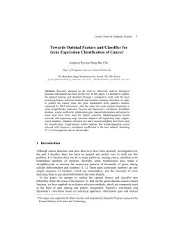


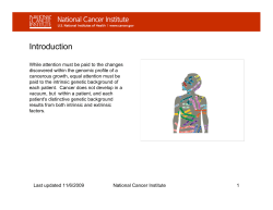

© Copyright 2026