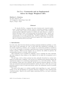
Author manuscript, published in "IEEE Transactions on Biomedical Engineering 58, 2 (2011) 355-362"
IEEE TRANSACTIONS ON BIOMEDICAL ENGINEERING, VOL. X, NO. Y, MONTH 2010
1
Regularizing Common Spatial Patterns to Improve
BCI Designs: Unified Theory and New Algorithms
inria-00476820, version 4 - 24 Sep 2010
Fabien LOTTE∗ , Member, IEEE, Cuntai GUAN, Senior Member, IEEE
Abstract—One of the most popular feature extraction algorithms for Brain-Computer Interfaces (BCI) is Common Spatial
Patterns (CSP). Despite its known efficiency and widespread use,
CSP is also known to be very sensitive to noise and prone to
overfitting. To address this issue, it has been recently proposed
to regularize CSP. In this paper, we present a simple and
unifying theoretical framework to design such a Regularized
CSP (RCSP). We then present a review of existing RCSP
algorithms, and describe how to cast them in this framework.
We also propose 4 new RCSP algorithms. Finally, we compare
the performances of 11 different RCSP (including the 4 new
ones and the original CSP), on EEG data from 17 subjects,
from BCI competition data sets. Results showed that the best
RCSP methods can outperform CSP by nearly 10% in median
classification accuracy and lead to more neurophysiologically
relevant spatial filters. They also enable us to perform efficient
subject-to-subject transfer. Overall, the best RCSP algorithms
were CSP with Tikhonov Regularization and Weighted Tikhonov
Regularization, both proposed in this paper.
Index Terms—brain-computer interfaces (BCI), EEG, common
spatial patterns (CSP), regularization, subject-to-subject transfer
I. I NTRODUCTION
Brain-Computer Interfaces (BCI) are communication systems which enable users to send commands to computers by
using brain activity only, this activity being generally measured
by ElectroEncephaloGraphy (EEG) [1]. BCI are generally
designed according to a pattern recognition approach, i.e., by
extracting features from EEG signals, and by using a classifier
to identify the user’s mental state from such features [1][2].
The Common Spatial Patterns (CSP) algorithm is a feature
extraction method which can learn spatial filters maximizing
the discriminability of two classes [3][4]. CSP has been proven
to be one of the most popular and efficient algorithms for BCI
design, notably during BCI competitions [5][6].
Despite its popularity and efficiency, CSP is also known
to be highly sensitive to noise and to severely overfit with
small training sets [7][8]. To address these drawbacks, a recent
idea has been to add prior information into the CSP learning
process, under the form of regularization terms [9][10][11][12]
(see Section IV-A for a review). These Regularized CSP
(RCSP) have all been shown to outperform classical CSP.
However, they are all expressed with different formulations
and therefore lack a unifying regularization framework. Moreover, they were only compared to standard CSP, and typically
with 4 or 5 subjects only [9][10][11], which makes it difficult
to assess their relative performances. Finally, we believe that
a variety of other priors could be incorporated into CSP.
F. Lotte and C. Guan are with the Institute for Infocomm Research, 1 Fusionopolis Way, 138632, Singapore. e-mail: fprlotte,[email protected]
Therefore, in this paper we present a simple theoretical
framework that could unify RCSP algorithms. We present
existing RCSP within this unified framework as well as 4 new
RCSP algorithms, based on new priors. It should be mentioned
that preliminary studies of 2 of these new algorithms have been
presented in conference papers [12][13]. Finally, we compare
these various algorithms on EEG data from 17 subjects, from
publicly available BCI competition data sets.
This paper is organized as follows: Section II describes the
CSP algorithm while Section III presents the theoretical framework to regularize it. Section IV expresses existing RCSP
within this framework and presents 4 new RCSP. Finally,
Sections V and VI describe the evaluations performed and
their results, and conclude the paper, respectively.
II. T HE CSP ALGORITHM
CSP aims at learning spatial filters which maximize the
variance of band-pass filtered EEG signals from one class
while minimizing their variance from the other class [4][3].
As the variance of EEG signals filtered in a given frequency
band corresponds to the signal power in this band, CSP aims
at achieving optimal discrimination for BCI based on band
power features [3]. Formally, CSP uses the spatial filters w
which extremize the following function:
w T C1 w
wT X1T X1 w
=
(1)
w T C2 w
wT X2T X2 w
where T denotes transpose, Xi is the data matrix for class
i (with the training samples as rows and the channels as
columns) and Ci is the spatial covariance matrix from class i,
assuming a zero mean for EEG signals. This last assumption is
generally met when EEG signals are band-pass filtered. This
optimization problem can be solved (though this is not the
only way) by first observing that the function J(w) remains
unchanged if the filter w is rescaled. Indeed J(kw) = J(w),
with k a real constant, which means the rescaling of w is arbitrary. As such, extremizing J(w) is equivalent to extremizing
wT C1 w subject to the constraint wT C2 w = 1 as it is always
possible to find a rescaling of w such that wT C2 w = 1. Using
the Lagrange multiplier method, this constrained optimization
problem amounts to extremizing the following function:
J(w) =
L(λ, w) = wT C1 w − λ(wT C2 w − 1)
(2)
The filters w extremizing L are such that the derivative of L
with respect to w equals 0:
∂L
= 2wT C1 − 2λwT C2 = 0
∂w
⇔ C1 w = λC2 w
⇔ C2−1 C1 w = λw
IEEE TRANSACTIONS ON BIOMEDICAL ENGINEERING, VOL. X, NO. Y, MONTH 2010
We obtain a standard eigenvalue problem. The spatial filters
extremizing Eq. 1 are then the eigenvectors of M = C2−1 C1
which correspond to its largest and lowest eigenvalues. When
using CSP, the extracted features are the logarithm of the EEG
signal variance after projection onto the filters w.
III. R EGULARIZED CSP: T HEORY
inria-00476820, version 4 - 24 Sep 2010
As mentioned above, to overcome the sensitivity of CSP
to noise and overfitting, one should regularize it. Adding prior
information to CSP, and thus regularizing it, can be done at two
levels. First, it can be done at the covariance matrix estimation
level. Indeed, CSP relying on covariance matrix estimates,
such estimates can suffer from noise or small training sets, and
thus benefit from regularization. Another approach consists in
regularizing CSP at the level of the objective function (Eq.
1), by imposing priors on the spatial filters to obtain. The
remaining of this section presents these two approaches.
A. Regularizing the covariance matrix estimates
CSP requires to estimate the spatial covariance matrix
for each class. However, if the EEG training set is noisy
and/or small, these covariance matrices may be poor or nonrepresentative estimates of the mental states involved, and thus
lead to poor spatial filters. Therefore, it is appropriate to add
prior information to these estimates by using regularization
terms. Based on [10], it can be performed as follows:
C̃c
=
(1 − γ)Ĉc + γI
(3)
with Ĉc
=
(1 − β)sc Cc + βGc
(4)
where Cc is the initial spatial covariance matrix for class
c, C̃c is the regularized estimate, I is the identity matrix,
sc is a constant scaling parameter (a scalar), γ and β are
two user-defined regularization parameters (γ, β ∈ [0, 1])
and Gc is a ”generic” covariance matrix (see below). Two
regularization terms are involved here. The first one, associated
to γ, shrinks the initial covariance matrix estimate towards
the identity matrix, to counteract a possible estimation bias
due to a small training set. The second term, associated to β,
shrinks the initial covariance matrix estimate towards a generic
covariance matrix, to obtain a more stable estimate. This
generic matrix represents a given prior on how the covariance
matrix for the mental state considered should be. This matrix
is typically built by using signals from several subjects whose
EEG data has been recorded previously. This has been shown
to be an effective way to perform subject-to-subject transfer
[11][10][13]. However, it should be mentioned that Gc could
also be defined based on neurophysiological priors only.
Learning spatial filters with this method simply consists in
replacing the covariance matrices C1 and C2 used in CSP by
their regularized estimates C̃1 and C̃2 . Many different RCSP
algorithms can be thus designed, depending on whether one
or both regularization terms are used, and more importantly,
on how the generic covariance matrix Gc is built.
2
B. Regularizing the CSP objective function
Another approach to obtain regularized CSP algorithms
consists in regularizing the CSP objective function itself
(Eq. 1). More precisely, such a method consists in adding
a regularization term to the CSP objective function in order
to penalize solutions (i.e., resulting spatial filters) that do not
satisfy a given prior. Formally, the objective function becomes:
JP1 (w) =
wT C1 w
+ αP (w)
wT C2 w
(5)
where P (w) is a penalty function measuring how much the
spatial filter w satisfies a given prior. The more w satisfies
it, the lower P (w). Hence, to maximize JP1 (w), we must
minimize P (w), thus ensuring spatial filters satisfying the
prior. α is a user-defined regularization parameter (α ≥ 0, the
higher α, the more satisfied the prior). With this regularization,
we expect that enforcing specific solutions, thanks to priors,
will guide the optimization process towards good spatial filters,
especially with limited or noisy training data.
In this paper, we focus on quadratic penalties: P (w) =
kwk2K = wT Kw, where matrix K encodes the prior. Interestingly enough, RCSP with non-quadratic penalties have been
proposed [14][15]. They used an l1 norm penalty to select
a sparse set of channels. However, these studies showed that
sparse CSP generally gave lower performances than CSP (with
all channels), although they require much less channels, hence
performing efficient channel reduction. As the focus of this
paper is not channel reduction but performance enhancement,
we only consider quadratic penalties here. Moreover, quadratic
penalties lead to a close form solution for optimization (see
below), which is more convenient and computationally efficient. With a quadratic penalty term, Eq. 5 becomes:
JP1 (w)
=
=
wT C1 w
wT C2 w + αwT Kw
wT C1 w
wT (C2 + αK)w
The corresponding Lagrangian is:
LP1 (λ, w) = wT C1 w − λ(wT (C2 + αK)w − 1)
(6)
By following the same approach as previously (see Section
II), we obtain the following eigenvalue problem:
(C2 + αK)−1 C1 w = λw
(7)
Thus, the filters w maximizing JP1 (w) are the eigenvectors
corresponding to the largest eigenvalues of M1 = (C2 +
αK)−1 C1 . With CSP, the eigenvectors corresponding to both
the largest and smallest eigenvalues of M (see Section II)
are used as the spatial filters, as they respectively maximize
and minimize Eq. 1 [4]. However, for RCSP, the eigenvectors
corresponding to the lowest eigenvalues of M1 minimize Eq.
5, and as such maximize the penalty term (which should be
minimized). Therefore, in order to obtain the filters which
maximize C2 while minimizing C1 , we also need to maximize
the following objective function:
JP2 (w) =
wT C2 w
wT C1 w + αP (w)
(8)
IEEE TRANSACTIONS ON BIOMEDICAL ENGINEERING, VOL. X, NO. Y, MONTH 2010
inria-00476820, version 4 - 24 Sep 2010
which is achieved by using the eigenvectors corresponding
to the largest eigenvalues of M2 = (C1 + αK)−1 C2 as the
filters w. In other words, with RCSP, the spatial filters used
are the eigenvectors corresponding to the largest eigenvalues of
M1 and to the largest eigenvalues of M2 . With this approach,
various regularized CSP algorithms can be designed depending
on the knowledge encoded into matrix K.
C. Summary
We have presented two theoretical approaches to design
RCSP algorithms: one at the covariance matrix estimation
level and one at the objective function level. Naturally, these
two approaches are not exclusive and can be combined within
the same framework. Table I summarizes this framework and
highlights the differences between CSP and RCSP. With this
framework, many different RCSP can be designed depending
on 1) which of the 3 regularization terms (associated to α, β
and γ) is (are) used and on 2) how the matrices Gc and K
are built. The following section presents several such variants,
including existing algorithms as well as 4 new ones.
TABLE I
D IFFERENCES IN OBJECTIVE FUNCTION AND ALGORITHM OPTIMIZATION
BETWEEN A STANDARD CSP AND A R EGULARIZED CSP (RCSP).
CSP
RCSP
wT C̃{1,2} w
wT C1 w
J(w) = T
JP{1,2} (w) =
w C2 w
wT C̃{2,1} w + αP (w)
Objective
with
function
P (w) = wT Kw
C̃c = (1 − γ)Ĉc + γI
Ĉc = (1 − β)sc Cc + βGc
eigenvectors
eigenvectors corresponding
Solutions
corresponding
to the Nf largest
of the
to the Nf largest
eigenvalues of
optimization and Nf lowest
M1 = (C̃2 + αK)−1 C̃1
problem
eigenvalues
and
of M = C2−1 C1
M2 = (C̃1 + αK)−1 C̃2
IV. R EGULARIZED CSP: A LGORITHMS
A. Existing RCSP algorithms
Four RCSP algorithms have been proposed so far:
Composite CSP, Regularized CSP with Generic Learning,
Regularized CSP with Diagonal Loading and invariant CSP.
They are described below within the presented framework.
1) Composite CSP:
The Composite CSP (CCSP) algorithm, proposed by Kang
et al [11], aims at performing subject-to-subject transfer by
regularizing the covariance matrices using other subjects’ data.
Expressed within the framework of this paper, CCSP uses only
the β hyperparameter (α = γ = 0), and defines the generic
covariance matrices Gc according to covariance matrices of
other subjects. Two methods were proposed to build Gc .
With the first method, denoted here as CCSP1, Gc is built
as a weighted sum of the covariance matrices (corresponding
to the same mental state) of other subjects, by de-emphasizing
covariance matrices estimated from fewer trials:
X Ni
Nc
c
Gc =
C i and sc =
(9)
Nt,c c
Nt,c
i∈Ω
3
where Ω is a set of subjects whose data is available, Cci is the
spatial covariance matrix for class c and subject i, Nci is the
number of EEG trials used to estimate Cci , Nc is the number of
EEG trials used to estimate Cc (matrix for the target subject),
and Nt,c is the total number of EEG trials for class c (from
all subjects in Ω together with the target subject).
With the second method, denoted as CCSP2, Gc is still a
weighted sum of covariance matrices from other subjects, but
the weights are defined according to the Kullback-Leibler (KL)
divergence between subjects’ data:
X
X 1
1
1
Cci with Z =
(10)
Gc =
Z KL(i, t)
KL(j, t)
i∈Ω
j∈Ω
where KL(i, t) is the KL-divergence between the target subject t and subject i, and is defined as follows:
det(Cc )
1
−1 i
log
+ tr(Cc Cc ) − Ne
(11)
KL(i, t) =
2
det(Cci )
where det and tr are respectively the determinant and the
trace of a matrix, and Ne is the number of electrodes used.
With CCSP2, the scaling constant sc is equal to 1.
2) Regularized CSP with Generic Learning:
The RCSP approach with Generic Learning, proposed by
Lu et al [10] and denoted here as GLRCSP, is another
approach which aims at regularizing the covariance matrix
estimation using data from other subjects. GLRCSP uses
both the β and γ regularization terms, i.e., it aims at
shrinking the covariance matrix towards both the identity
matrix and a generic covariance matrix Gc . Similarly to
CCSP, Gc is here computed from the covariance
matrices
P
of other subjects such that Gc = sG i∈Ω Cci , where
1 P
sc = sG = (1−β)MC +β
, and MC is the number of
i
c
i∈Ω MCc
trials used to compute the covariance matrix C.
3) Regularized CSP with Diagonal Loading:
Another form of covariance matrix regularization used in the
BCI literature is Diagonal Loading (DL), which consists in
shrinking the covariance matrix towards the identity matrix.
Thus, this approach only uses the γ regularization parameter
(β = α = 0). Interestingly enough, in this case the value of
γ can be automatically identified using Ledoit and Wolf’s
method [16]. We denote this RCSP based on automatic
DL as DLCSPauto. In order to check the efficiency of this
automatic regularization for discrimination purposes, we
will also investigate a classical selection of γ using crossvalidation. We denote the resulting algorithm as DLCSPcv.
When using Ledoit and Wolf’s method for automatic
regularization, the value of γ selected to regularize C1 can
be different than that selected to regularize C2 . Therefore,
we also investigated cross-validation to select a potentially
different regularization parameter for C1 and C2 . We denote
this method as DLCSPcvdiff. To summarize, DLCSPauto
automatically selects two γ regularization parameters (one
for C1 and one for C2 ) ; DLCSPcv selects a single γ
regularization parameter for both C1 and C2 using cross
validation ; finally, DLCSPcvdiff selects two γ regularization
parameters (one for C1 and one for C2 ) using cross
IEEE TRANSACTIONS ON BIOMEDICAL ENGINEERING, VOL. X, NO. Y, MONTH 2010
inria-00476820, version 4 - 24 Sep 2010
validation. It should be mentioned that, although covariance
matrix regularization based on DL has been used in the BCI
literature (see, e.g., [17]), to our best knowledge, it has not
been used for CSP regularization, but for regularization of
other algorithms such as Linear Discriminant Analysis (LDA).
4) Invariant CSP:
Invariant CSP (iCSP), proposed by Blankertz et al [9], aims at
regularizing the CSP objective function in order to make filters
invariant to a given noise source (it uses β = γ = 0). To do
so, the regularization matrix K is defined as the covariance
matrix of this noise source, e.g., as the covariance matrix of the
changing level of occipital α-activity. It should be mentioned
that, to obtain this noise covariance matrix, additional EEG
measurements must be performed to acquire the corresponding
EEG signals and compute their covariance matrix. Since such
measurements are not available for the EEG data sets analyzed
here, iCSP will not be considered for evaluation in this paper.
However, it still seems to be an efficient approach to make
CSP robust against known noise sources.
B. New RCSP algorithms
In this section, we propose 4 new algorithms to regularize
CSP: a CSP regularized with selected subjects, a Tikhonov
Regularized CSP, a weighted Tikhonov Regularized CSP and
a spatially Regularized CSP.
1) Regularized CSP with Selected Subjects:
This first new RCSP belongs to the same family as CCSP
since it uses data from other subjects to shrink the covariance
matrix towards a generic matrix Gc (it uses β ≥ 0 and α =
γ = 0). However, contrary to CCSP or GLRCSP, the proposed
algorithm does not use the data from all available subjects but
only from selected subjects. Indeed, even if data from many
subjects is available, it may not be relevant to use all of them,
due to potentially large inter-subject variabilities. Thus, we
propose to build Gc from the covariance matrices of a subset of
selected subjects. We therefore denote this algorithm as RCSP
with Selected Subjects or SSRCSP. With SSRCSP,
Pthe generic
covariance matrix is defined as Gc = |St 1(Ω)| i∈St (Ω) Cci ,
where |A| is the number of elements in set A and St (Ω) is
the subset of selected subjects from Ω.
To select an appropriate subset of subjects St (Ω),
we propose the subject selection algorithm described
in Algorithm 1. In this algorithm, the function
accuracy = trainT henT est(trainingSet, testingSet)
returns the accuracy obtained when training an SSRCSP
with β = 1 (i.e., using only data from other subjects) on
the data set trainingSet and testing it on data set testingSet,
with an LDA as classifier. The function (besti , maxf (i) ) =
maxi f (i) returns besti , the value of i for which f (i) reaches
its maximum maxf (i) . In short, this algorithm sequentially
selects the subject to add or to remove from the current subset
of subjects, in order to maximize the accuracy obtained when
training the BCI on the data from this subset of subjects
and testing it on the training data of the target subject. This
algorithm has the same structure as the Sequential Forward
4
Floating Search algorithm [18], used to select a relevant subset
of features. This ensures the convergence of our algorithm
as well as the selection of a good subset of additional subjects.
Input: Dt : training EEG data from the target subject.
Input: Ω = {Ds }, s ∈ [0, Ns ]: set of EEG data from the Ns
other subjects available (Dt 3 Ω).
Output: St (Ω): a subset of relevant subjects whose data can be
used to classify the data Dt of the target subject.
selected0 = {};
remaining0 = Ω;
accuracy0 = 0; n = 1;
while n < Ns do
Step 1: (bestSubject, bestAccuracy) =
maxs∈remainingn−1 trainT henT est(selectedn−1 +
{Ds }, Dt );
selectedn = selectedn−1 + {DbestSubject };
remainingn = remainingn−1 - {DbestSubject };
accuracyn = bestAccuracy;
n = n + 1;
Step 2: if n > 2 then
(bestSubject, bestAccuracy) =
maxs∈selectedn trainT henT est(selectedn −
{Ds }, Dt );
if bestAccuracy > accuracyn−1 then
selectedn−1 = selectedn - {DbestSubject };
remainingn−1 = remainingn + {DbestSubject };
accuracyn−1 = bestAccuracy;
n = n − 1;
go to Step 2;
else
go to Step 1;
end
end
end
(bestN, selectedAcc) = maxn∈[1,Ns ] accuracyn ;
St (Ω) = selectedbestN ;
Algorithm 1: Subject selection algorithm for the SSRCSP
(Regularized CSP with Selected Subjects) algorithm.
2) CSP with Tikhonov Regularization:
The next new algorithms we propose are based on the
regularization of the CSP objective function using quadratic
penalties (with α ≥ 0, γ = β = 0 and sc = 1). The first
one is a CSP with Tikhonov Regularization (TR) or TRCSP.
Tikhonov Regularization is a classical form of regularization,
initially introduced for regression problems [19], and which
consists in penalizing solutions with large weights. The
penalty term is then P (w) = kwk2 = wT w = wT Iw. TRCSP
is then simply obtained by using K = I in the proposed
framework (see Table I). Such regularization is expected to
constrain the solution to filters with a small norm, hence
mitigating the influence of artifacts and outliers.
3) CSP with Weighted Tikhonov Regularization:
With TRCSP, high weights are penalized equally for each
channel. However, we know that some channels are more
important than others to classify a given mental state. Thus,
it may be interesting to have different penalties for different
channels. If we believe that a channel is unlikely to have a
large contribution in the spatial filters, then we should give it a
relatively large penalty, in order to prevent CSP from assigning
IEEE TRANSACTIONS ON BIOMEDICAL ENGINEERING, VOL. X, NO. Y, MONTH 2010
it a large contribution (which can happen due to artifacts for
instance). On the other hand, if a channel is likely to be useful,
we should not prevent CSP from giving it high weights, as this
channel is likely to have a genuinely large contribution.
Formally, this leads to a penalty term of the form P (w) =
wT Dw w, where Dw is a diagonal matrix such that Dw =
diag(wG ) and wG (i) is the level of penalty assigned to
channel i. Weighted Tikhonov Regularized CSP (WTRCSP) is
then obtained by using K = Dw . These penalty levels wG (i)
can be defined according to the literature, i.e., according to
which brain regions (and thus channels) are expected to be
useful. However, it may be difficult to select manually an
appropriate penalty value for each channel. In this paper, we
therefore use data from other subjects to obtain wG :

−1
2×Nf i X
X
w
1
f 
(12)
wG = 
i kwf k 2 × Nf × |Ω|
inria-00476820, version 4 - 24 Sep 2010
i∈Ω f =1
where wfi is the f th spatial filter obtained using CSP (among
the eigenvectors corresponding to the Nf largest and lowest
eigenvalues of M , see Table I) for the ith additional subject
available. In other words, the penalty level of a channel is set
to the inverse of the average absolute value of the normalized
weight of this channel in the CSP filters obtained from other
subjects (the less important the average channel weight,
the higher the penalty). By doing so, we expect that the
degree of usefulness of a given channel would be reflected by
its weight in the filters obtained with CSP from other subjects.
4) Spatially Regularized CSP:
The last algorithm we propose is a Spatially Regularized CSP
(SRCSP). The motivation behind this algorithm is that despite
being used to learn spatial filters, CSP completely ignores the
spatial location of EEG electrodes. SRCSP aims at making
use of this spatial information. More particularly, we would
like to obtain spatially smooth filters w, i.e, filters for which
neighboring electrodes have relatively similar weights. Indeed,
from a neurophysiological point of view, neighboring neurons
tend to have similar functions, which supports the idea that
neighboring electrodes should measure similar brain signals
(if they are close enough to each other). To ensure spatial
smoothness of the filters w, we use a Laplacian penalty term
P (w) as in [20], with the following regularization matrix K:
1 kvi − vj k2
) (13)
2
r2
where vi is the vector containing the 3D coordinates of the
th
iP
electrode, and DG is a diagonal matrix such as DG (i, i) =
j G(i, j). Here, r is a hyperparameter which defines how far
two electrodes can be to beP
still considered as close to each
other. As wT (DG − G)w = i,j G(i, j)(wi − wj )2 (see, e.g.,
[21]), the penalty term P (w) = wT Kw will be large for nonsmooth filters, i.e., for filters in which neighboring electrodes
have very different weights.
K = DG − G with G(i, j) = exp(−
C. Hyperparameter selection
All RCSP algorithms presented here (expect DLCSPauto)
have one or more regularization parameters whose value must
5
be defined by the user: α, β and γ (see Table I). SRCSP
has also its own specific hyperparameter: r which defines
the size of the neighborhood considered for smoothing. In
[10] and [11], the selection of the regularization parameters
for GLRCSP and CCSP was not addressed, and the authors
presented the results for several values of the hyperparameters.
In this paper, we used cross-validation (CV) to select these
values. More precisely, we used as optimal hyperparameter
values, those that maximized the 10-fold cross validation
accuracy on the training set by using LDA [2] as classifier.
We selected values among the set [0, 0.1, 0.2, . . . , 0.9] for the
parameters β and γ, among the set [10−10 , 10−9 , . . . , 10−1 ]
for α, and among [0.01, 0.05, 0.1, 0.5, 0.8, 1.0, 1.2, 1.5] for r.
D. The best of two worlds?
So far, all the algorithms presented use a single form of
regularization: either they regularize the covariance matrices
or the objective function, but not both. However, it is easy
to imagine an algorithm combining these two approaches.
We evaluated some such algorithms, e.g., a SRCSP with
Diagonal Loading or a TRCSP with Generic Learning, among
others. Unfortunately, none of them reached performances
as high as that of the corresponding RCSP with a single
form of regularization (results not reported here due to space
limitations). Thus, it seems that RCSP with a single form of
regularization are the simplest and most efficient algorithms.
V. E VALUATION
A. EEG data sets used for evaluation
In order to assess and compare the RCSP algorithms presented here, we used EEG data from 17 subjects, from 3
publicly available data sets of BCI competitions. These three
data sets contain Motor Imagery (MI) EEG signals, i.e., EEG
signals recorded while subjects imagine limb movements (e.g.,
hand or foot movements) [1]. They are described below.
1) Data set IVa, BCI competition III: Data set IVa [22],
from BCI competition III [6], contains EEG signals from 5
subjects, who performed right hand and foot MI. EEG were
recorded using 118 electrodes. A training set and a testing set
were available for each subject. Their size was different for
each subject. More precisely, 280 trials were available for each
subject, among which 168, 224, 84, 56 and 28 composed the
training set for subject A1, A2, A3, A4 and A5 respectively,
the remaining trials composing their test set.
2) Data set IIIa, BCI competition III: Data set IIIa [23],
from BCI competition III [6], comprises EEG signals from 3
subjects who performed left hand, right hand, foot and tongue
MI. EEG signals were recorded using 60 electrodes. For the
purpose of this study, only EEG signals corresponding to left
and right hand MI were used. A training and a testing set were
available for each subject. Both sets contain 45 trials per class
for subject B1, and 30 trials per class for subjects B2 and B3.
3) Data set IIa, BCI competition IV: Data set IIa [24], from
BCI competition IV1 comprises EEG signals from 9 subjects
who performed left hand, right hand, foot and tongue MI. EEG
1 http://www.bbci.de/competition/iv/
IEEE TRANSACTIONS ON BIOMEDICAL ENGINEERING, VOL. X, NO. Y, MONTH 2010
signals were recorded using 22 electrodes. Only EEG signals
corresponding to left and right hand MI were used for the
present study. A training and a testing set were available for
each subject, both sets containing 72 trials for each class.
B. Preprocessing
In this work, we considered the discrete classification of
the trials, i.e., we assigned a class to each trial. For each
data set and trial, we extracted features from the time segment
located from 0.5s to 2.5s after the cue instructing the subject
to perform MI (as done by the winner of BCI competition IV,
data set IIa). Each trial was band-pass filtered in 8-30 Hz, as
in [3], using a 5th order Butterworth filter. With each (R)CSP
algorithm, we used 3 pairs of filters for feature extraction
(Nf = 3), as recommended in [4].
inria-00476820, version 4 - 24 Sep 2010
C. Results and discussion
For each subject, the (R)CSP filters were learnt on the
training set available. The log-variances of the spatially filtered
EEG signals were then used as input features to an LDA, one
of the most efficient classifiers for BCI [2]. Table II reports
on the classification accuracies obtained on the test sets.
Results show that, except DLCSPauto and CCSP2, all RCSP
algorithms outperformed classical CSP, often substantially.
The best RCSP algorithms outperformed CSP by about 3 to
4% in mean classification accuracy and by almost 10% in
median classification accuracy. This confirms that when using
CSP, regularization should be used in order to deal with its
non-robust nature. The performance variance is also lower
for RCSP algorithms. This, together with a closer look at
the results, suggests that RCSP algorithms are more valuable
for subjects with poor initial performances (e.g., A3, A5, B2,
C5), than for already good subjects, whose performances are
roughly unchanged. This makes sense as regularization aims
at dealing with noisy or limited data, but not necessarily at
improving performances for already good and clean data.
The best RCSP algorithm on these data is the WTRCSP
that we proposed in this paper, as it reached both the highest
median and mean accuracy. It is only slightly better than
TRCSP, also proposed in this paper. These two algorithms have
only a single hyperparameter to tune (α), which makes them
more convenient to use and more computationally efficient
than other good RCSP algorithms such as GLRCSP or SRCSP,
which both have two hyperparameters.
In terms of statistical significance, a Friedman test [25][26]
revealed that the RCSP algorithm used had a significant effect
on the classification performance, at the 5% level (p = 0.03).
It should be noted that we used the Friedman test because it is
a non-parametric equivalent of the repeated measure ANOVA.
Indeed, the fact that the mean and median accuracies are
rather different in our data suggests that the accuracy may
not be normally distributed. This makes the use of ANOVA
inappropriate [25]. Post-hoc multiple comparisons revealed
that TRCSP is significantly more efficient than CSP and DLCSPcvdiff. Actually, TRCSP appeared as the only algorithm
which is significantly more efficient than CSP. However, other
RCSP also seem more efficient than CSP but perhaps not
6
significantly so due to the relatively modest sample size. Both
TRCSP and WTRCSP appeared as significantly more efficient
than GLRCSP, CCSP1, CCSP2 and DLCSPcv. Finally, SRCSP
was significantly more efficient than CCSP1 and DLCSPcv.
In general, regularizing the CSP objective function seems
more rewarding, in terms of performances, than regularizing
the covariance matrices. A possible explanation might be
found in Vapnik’s statistical learning theory which advocates
that “when solving a given problem, try to avoid solving a
more generic problem as an intermediate step” [27]. Indeed,
the objective of RCSP algorithms is to promote the learning
of good spatial filters. However, when using covariance matrix
regularization, we try to solve the more generic intermediate
problem of obtaining a good covariance matrix estimate. We
then hope this will lead to better spatial filters even though
this was not directly addressed. On the other hand, when
regularizing the objective function, we directly try to learn
better spatial filters by enforcing some good prior structures
for these filters. This might be an explanation as to why the
latter approach is generally more efficient than the former.
Results obtained by CCSP, GLRCSP, SSRCSP and
WTRCSP showed that subject-to-subject transfer in BCI is
possible and valuable. Despite large inter-subject variabilities,
knowing that using data from other subjects can improve
performances may also benefit other EEG signal processing
algorithms. Among RCSP methods using only data from other
subjects to regularize the covariance matrices (i.e., CCSP1,
CCSP2 and SSRCSP), SSRCSP reached the highest mean
accuracy, which suggests that it is worth selecting subjects
to build Gc . However, overall, WTRCSP appears as the most
efficient algorithm that exploits subject-to-subject transfer.
Nevertheless, since RCSP algorithms based on subject-tosubject transfer require EEG data from additional subjects,
it may not always be possible to use them. Indeed, the performance improvement they offer may not justify the additional
time required to collect data from new subjects. However, if
data from other subjects is already available, which is likely
to be the case if a given BCI system has been used for
some times, then such RCSP algorithms are worth being used.
Moreover, our study used a rather small number of additional
subjects (2 to 8 depending on the data set). With a larger data
base of additional subjects, performance improvements due to
subject-to-subject transfer may be even larger (see, e.g., [28]).
Concerning the poor performances of DLCSPauto, it should
be mentioned that we also observed poor performance when
all training data were used in one of our previous studies
[13]. However, when using this approach with a small training
set, DLCSPauto proved to be significantly more efficient than
CSP. This suggests DLCSPauto is most useful when very little
training data is available. A comparison of DLCSPcv with
DLCSPcvdiff showed that they obtained very similar performances. Actually, for 13 subjects out of 17, DLCSPcvdiff
selected the same value for the regularization parameters of
C1 and C2 , i.e., it was equivalent to DLCSPcv. This suggests
that it may not be necessary to use different regularization
parameter values for each covariance matrix.
The fact that RCSP algorithms led to lower scores than
CSP on a few subjects is also surprising. Indeed, if the best
IEEE TRANSACTIONS ON BIOMEDICAL ENGINEERING, VOL. X, NO. Y, MONTH 2010
7
TABLE II
C LASSIFICATION ACCURACIES ( MEAN , MEDIAN AND STANDARD DEVIATION ( STD ) IN %) OBTAINED FOR EACH SUBJECT FOR THE STANDARD CSP AND
THE R EGULARIZED CSP ALGORITHMS PRESENTED IN THIS PAPER . F OR EACH SUBJECT, THE BEST RESULT IS DISPLAYED IN BOLD CHARACTERS .
inria-00476820, version 4 - 24 Sep 2010
Subject
CSP
GLRCSP
CCSP1
CCSP2
DLCSPauto
DLCSPcv
DLCSPcvdiff
SSRCSP
TRCSP
WTRCSP
SRCSP
A1
66.07
72.32
66.96
65.18
66.96
64.29
69.64
70.54
71.43
69.64
72.32
BCI competition
data set IVa
A2
A3
A4
A5
96.43 47.45 71.88 49.6
96.43 66.84 67.86 89.29
96.43 63.27 71.88 84.92
96.43 45.41 71.88 49.6
96.43 46.94 71.43 50
96.43 52.04 71.88 82.54
98.21 55.1 71.88 82.54
96.43 53.57 71.88 75.39
96.43 63.27 71.88 86.9
98.21 54.59 71.88 85.32
96.43 60.2 77.68 86.51
III
data set IIIa
B1
B2
B3
95.56 61.67 93.33
95.56 61.67 90
98.89 45 93.33
95.56 61.67 93.33
94.44 63.33 95
95.56 78.33 93.33
95.56 66.67 93.33
95.56 61.67 96.67
98.89 56.67 93.33
98.89 71.67 93.33
96.67 53.33 93.33
C1
88.89
86.11
86.11
88.89
88.89
88.89
88.89
88.89
88.89
88.89
88.89
results could be obtained without regularization, then we could
expect that the hyperparameter selection procedure based on
cross-validation would figure it out and set the regularization
parameter to 0. However, it sometimes seemed otherwise. This
may suggest that, perhaps due to the non-stationarity of EEG,
cross-validation is not a very good predictor of generalization
performances for BCI. This has been also observed in one
subject in [9]. We will investigate this issue in the future.
Figure 1 shows some examples of spatial filters obtained
with different (R)CSP algorithms for different subjects. In
general, these pictures show that CSP filters appear as messy,
with large weights in several unexpected locations from a
neurophysiological point of view. On the contrary, RCSP filters
are generally smoother and physiologically more relevant, with
strong weights over the motor cortex areas, as expected from
the literature [1]. This suggests that another benefit of RCSP
algorithms is to lead to filters that are neurophysiologically
more plausible and as such more interpretable.
Fig. 1. Electrode weights for corresponding filters obtained with different
CSP algorithms (CSP, GLRCSP, SRCSP and WTRCSP), for subjects A1, A5
(118 electrodes), B2 (60 electrodes) and C6, C9 (22 electrodes).
C2
51.39
58.33
60.42
53.47
51.39
50.69
50.69
53.47
54.17
54.86
63.19
C3
96.53
93.75
93.75
97.22
96.53
96.53
96.53
97.22
96.53
96.53
96.53
BCI competition IV
data set IIa
C4
C5
C6
70.14 54.86 71.53
67.36 55.56 65.28
56.94 49.31 65.28
70.14 54.17 68.06
70.14 56.94 71.53
70.14 55.56 62.5
70.14 55.56 62.5
70.14 56.25 68.75
70.83 62.5 67.36
70.14 65.97 61.81
66.67 63.19 63.89
Overall
C7
81.25
81.25
81.25
79.17
81.94
81.25
81.25
79.17
81.25
81.25
78.47
C8
93.75
93.75
93.75
95.14
93.75
93.75
93.75
97.22
95.87
95.83
95.83
C9 Mean Median Std
93.75 75.5 71.9 18.2
88.19 78.2 81.3 14.3
88.19 76.2 81.3 17.5
90.28 75
71.9 18.3
93.75 75.9 71.5
18
86.81 77.7 81.3 16.1
86.81 77.6 81.3
16
90.28 77.8 75.4 16.2
91.67 79.3 81.3 15.3
90.97 79.4 81.3 15.3
92.36 79.2 78.5 15.2
VI. C ONCLUSION
In this paper, we proposed a unified theoretical framework
to design Regularized CSP. We proposed a review of existing
RCSP algorithms, and presented how to cast them in this
framework. We also proposed 4 new RCSP algorithms. We
evaluated 11 different RCSP algorithms (including the 4 new
ones and the original CSP), on EEG data from 17 subjects,
from BCI competition data sets. Results showed that the best
RCSP can outperform CSP by almost 10% in median classification accuracy and lead to more neurophysiologically relevant
spatial filters. They also showed that RCSP can perform
efficient subject-to-subject transfer. Overall, the best RCSP on
these data were WTRCSP and TRCSP, both newly proposed
in this paper. Therefore, we would recommend BCI designers
using CSP to adopt RCSP algorithms in order to obtain more
robust systems. To encourage such an adoption and to ensure
the present study replicability, a Matlab toolbox with all CSP
algorithms evaluated in this paper is freely available upon
request to the authors (e-mail: [email protected]).
Future work could deal with investigating performances
of RCSP algorithms with very small training sets, so as to
reduce BCI calibration time, in the line of our previous studies
[13][29]. It could also be interesting to adapt the presented
regularization framework to multiclass CSP approaches based
on approximate joint diagonalization such as [30]. We could
also cast the problem of subject-to-subject transfer for RCSP
as a multitask problem. In this case, the mean and/or variance
of spatial filters learnt across multiple subjects would be used
as prior information, in a similar flavor as what has been
done in [31] for learning linear classifiers. Finally, we could
explore the integration of the regularization terms proposed
here into one-step procedures, which learn the spatial filter
and the classifier simultaneously, as in [32].
Acknowledgments: The authors would like to thank Dr.
Schlögl and Dr. Blankertz for providing the electrode coordinates of BCI competition data, and Dr. Hamadicharef, Ms.
Rosendale and anonymous reviewers for their constructive
comments.
IEEE TRANSACTIONS ON BIOMEDICAL ENGINEERING, VOL. X, NO. Y, MONTH 2010
inria-00476820, version 4 - 24 Sep 2010
R EFERENCES
[1] G. Pfurtscheller and C. Neuper, “Motor imagery and direct braincomputer communication,” proc IEEE, vol. 89, no. 7, pp. 1123–1134,
2001.
[2] F. Lotte, M. Congedo, A. Lécuyer, F. Lamarche, and B. Arnaldi,
“A review of classification algorithms for EEG-based brain-computer
interfaces,” J Neural Eng, vol. 4, pp. R1–R13, 2007.
[3] H. Ramoser, J. Muller-Gerking, and G. Pfurtscheller, “Optimal spatial
filtering of single trial EEG during imagined hand movement,” IEEE
Trans Rehab Eng, vol. 8, no. 4, pp. 441–446, 2000.
[4] B. Blankertz, R. Tomioka, S. Lemm, M. Kawanabe, and K.-R. Müller,
“Optimizing spatial filters for robust EEG single-trial analysis,” IEEE
Signal Proc Magazine, vol. 25, no. 1, pp. 41–56, 2008.
[5] B. Blankertz, K. R. Müller, G. Curio, T. M. Vaughan, G. Schalk,
J. R. Wolpaw, A. Schlögl, C. Neuper, G. Pfurtscheller, T. Hinterberger,
M. Schröder, and N. Birbaumer, “The BCI competition 2003: Progress
and perspectives in detection and discrimination of EEG single trials,”
IEEE Trans Biomed Eng, vol. 51, no. 6, pp. 1044–1051, 2004.
[6] B. Blankertz, K. R. Müller, D. J. Krusienski, G. Schalk, J. R. Wolpaw,
A. Schlögl, G. Pfurtscheller, J. D. R. Mı́llan, M. Schroder, and N. Birbaumer, “The BCI competition III: Validating alternative approaches to
actual BCI problems,” IEEE Trans Neural Syst Rehab, vol. 14, no. 2,
pp. 153–159, 2006.
[7] B. Reuderink and M. Poel, “Robustness of the common spatial patterns
algorithm in the BCI-pipeline,” University of Twente, Tech. Rep., 2008.
[8] M. Grosse-Wentrup, C. Liefhold, K. Gramann, and M. Buss, “Beamforming in non invasive brain computer interfaces,” IEEE Trans Biomed
Eng, vol. 56, no. 4, pp. 1209 – 1219, 2009.
[9] B. Blankertz, M. Kawanabe, R. Tomioka, F. Hohlefeld, V. Nikulin, and
K.-R. Müller, “Invariant common spatial patterns: Alleviating nonstationarities in brain-computer interfacing,” in NIPS 20, 2008.
[10] H. Lu, K. Plataniotis, and A. Venetsanopoulos, “Regularized common
spatial patterns with generic learning for EEG signal classification,” in
EMBC, 2009, pp. 6599 – 6602.
[11] H. Kang, Y. Nam, and S. Choi, “Composite common spatial pattern for
subject-to-subject transfer,” IEEE Sig Proc Let, vol. 16, no. 8, pp. 683
– 686, 2009.
[12] F. Lotte and C. Guan, “Spatially regularized common spatial patterns
for EEG classification,” in ICPR, 2010, pp. 3712–3715.
[13] ——, “Learning from other subjects helps reducing brain-computer
interface calibration time,” in ICASSP, 2010, pp. 614–617.
[14] J. Farquhar, N. Hill, T. Lal, and B. Schölkopf, “Regularised CSP for
sensor selection in BCI,” in 3rd international BCI workshop, 2006.
[15] X. Yong, R. Ward, and G. Birch, “Sparse spatial filter optimization for
EEG channel reduction in brain-computer interface,” in ICASSP, 2008,
pp. 417–420.
[16] O. Ledoit and M. Wolf, “A well-conditioned estimator for largedimensional covariance matrices,” J Multivariate Analysis, vol. 88, no. 2,
pp. 365–411, 2004.
[17] C. Vidaurre, N. Krämer, B. Blankertz, and A. Schlögl, “Time domain
parameters as a feature for EEG-based brain computer interfaces,”
Neural Networks, vol. 22, pp. 1313–1319, 2009.
[18] P. Pudil, F. J. Ferri, and J. Kittler, “Floating search methods for feature
selection with non monotonic criterion functions,” Patt Recog, vol. 2,
pp. 279–283, 1994.
[19] A. Tikhonov, “Regularization of incorrectly posed problems,” Soviet
Math., vol. 4, pp. 1624–1627, 1963.
[20] Z. Xiang, Y. Xi, U. Hasson, and P. Ramadge, “Boosting with spatial
regularization,” in NIPS, 2009.
[21] D. Cai, X. He, Y. Hu, J. Han, and T. Huang, “Learning a spatially
smooth subspace for face recognition,” in CVPR, 2007.
[22] G. Dornhege, B. Blankertz, G. Curio, and K. Müller, “Boosting bit rates
in non-invasive EEG single-trial classifications by feature combination
and multi-class paradigms,” IEEE Trans Biomed Eng, vol. 51, no. 6, pp.
993–1002, 2004.
[23] A. Schlögl, F. Lee, H. Bischof, and G. Pfurtscheller, “Characterization
of four-class motor imagery EEG data for the BCI-competition 2005,”
J Neural Eng, pp. L14–L22, 2005.
[24] M. Naeem, C. Brunner, R. Leeb, B. Graimann, and G. Pfurtscheller,
“Seperability of four-class motor imagery data using independent components analysis,” J Neural Eng, vol. 3, pp. 208–216, 2006.
[25] P. Sprent and N. Smeeton, Applied nonparametric statistical methods.
Chapman & Hall, 2001.
[26] G. Cardillo. (2009) Myfriedman: Friedman test for non parametric
repeated measure analysis of variance. [Online]. Available: http:
//www.mathworks.com/matlabcentral/fileexchange/25882
8
[27] V. Vapnik, The Nature of Statistical Learning Theory, Second edition.
Springer-Verlag, New-York, 2000.
[28] S. Fazli, F. Popescu, M. Danóczy, B. Blankertz, K.-R. Müller, and
C. Grozea, “Subject-independent mental state classification in single
trials,” Neural Networks, vol. 22, no. 9, pp. 1305–1312, 2009.
[29] F. Lotte and C. Guan, “An efficient P300-based brain-computer interface
with minimal calibration time,” in AMD-NIPS, 2009.
[30] M. Grosse-Wentrup and M. Buss, “Multi-class common spatial pattern
and information theoretic feature extraction,” IEEE Trans on Biomed
Eng, vol. 55, no. 8, pp. 1991–2000, 2008.
[31] M. Alamgir, M. Grosse-Wentrup, and Y. Altun, “Multitask learning for
brain-computer interfaces,” in AISTATS, 2010, pp. 17–24.
[32] R. Tomioka and K.-R. Müller, “A regularized discriminative framework
for EEG analysis with application to brain-computer interface,” Neuroimage, vol. 49, no. 1, pp. 415–432, 2010.
Fabien LOTTE obtained a M.Sc., a M.Eng. and a
PhD degree in computer sciences, all from the National Institute of Applied Sciences (INSA) Rennes,
France, in 2005 and 2008 respectively. As a PhD
candidate he was part of the French National Research Institute for Computer Science and Control (INRIA) and was supervised by Dr. Anatole
LECUYER and Pr. Bruno ARNALDI. His PhD Thesis received both the PhD Thesis award 2009 from
AFRIF (French Association for Pattern Recognition)
and the PhD Thesis award 2009 accessit (2nd prize)
from ASTI (French Association for Information Sciences and Technologies).
In October and November 2008, he was a visiting PhD student at the HIROSETANIKAWA laboratory, the University of Tokyo, Japan. Since January 2009,
he works as a research fellow in Singapore, at the Institute for Infocomm Research (I2R), Signal processing department, in the Brain-Computer Interface
laboratory lead by Dr. Cuntai GUAN. His research interests include braincomputer interfaces, pattern recognition, virtual reality and signal processing.
Cuntai GUAN is a Principal Scientist & Program Manager at Institute for Infocomm Research,
Agency for Science, Technology and Research, Singapore. He received the Ph.D. degree in electrical
and electronic engineering from Southeast University, China, in 1993. From 1993 to 1994, he was at
the Southeast University, where he worked on speech
vocoder, speech recognition, and text-to-speech. In
1995, he was a Visiting Scientist at the Centre de
Recherche en Informatique de Nancy, France, where
he was working on key word spotting. From 1996
to 1997, he was with the City University of Hong Kong, where he was
developing robust speech recognition under noisy environment. From 1997 to
1999, he was with the Kent Ridge Digital Laboratories, Singapore, where he
was working on multilingual, large vocabulary, continuous speech recognition.
He was then a Research Manager and the R&D Director for five years in
industries, focusing on the research and development of spoken dialogue
technologies. Since 2003, he established the Brain-computer Interface Laboratory at Institute for Infocomm Research. He has published over 90 refereed
journal and conference papers, and holds 8 granted patents and applications.
He is Associate Editor of Frontiers in Neuroprosthetics. He is a Senior
Member of the IEEE, and President of Pattern Recognition and Machine
Intelligence Association (PREMIA), Singapore. His current research interests
include brain-computer interface, neural signal processing, machine learning,
pattern classification, and statistical signal processing, with applications to
neuro-rehabilitation, health monitoring, and cognitive training.