
Modeling Nanopores for Sequencing DNA
Modeling Nanopores for Sequencing DNA
Jeffrey R. Comer
David B. Wells
Aleksei Aksimentiev
July 2, 2015
Abstract
Using nanopores to sequence DNA rapidly and at a low cost has the potential to radically
transforms the field of genomic research. However, despite all the exciting developments in
the field, sequencing DNA using a nanopore has yet to be demonstrated. Among the many
problems that hinder development of the nanopore sequencing methods is the inability of current
experimental techniques to visualize DNA conformations in a nanopore and directly relate the
microscopic state of the system to the measured signal. We have recently shown that such tasks
could be accomplished through computation. This chapter provides step-by-step instructions
of how to build atomic scale models of biological and solid-state nanopore systems, use the
molecular dynamics method to simulate the electric field-driven transport of ions and DNA
through the nanopores, and analyze the results of such computational experiments.
Key words: Molecular dynamics, transmembrane transport, nucleic acids, membrane proteins,
bionanotechnology, computer simulations.
1
Introduction
The successful completion of the human genome project created the opportunity for even more
ambitious endeavors in the field of genomic research. For example, the personal genome project aims
to establish the relationship between the variations in the DNA sequence among individuals and
their health conditions and response to drugs and treatments. The goal of the cancer genome atlas
project is to determine which DNA mutations lead to cancer in different human organs and tissues.
To make whole-genome sequencing a routine procedure, the time and cost of sequencing must be
further reduced by two orders of magnitude or more to less than a day and $1000, respectively.
Among many new approaches to sequencing DNA that are being explored, the so-called nanopore
methods promise the most radical reduction in sequencing time and cost ( 1 ). In a typical nanopore
measurement, negatively charged DNA is driven through a nanometer-sized pore in a nanometerthick membrane by applying a voltage difference. As DNA passes through the nanopore, the sequence of nucleotides is detected by a readout mechanism. This enables detection of the nucleotide
sequence directly from the DNA strand, requiring small amounts of reagents, simple sample preparation procedures and having no limit on the length of the DNA fragment that can be read in
one measurement. At present, several types of observable signals are being explored as a readout
mechanism for nanopore sequencing, including transverse tunnelling current ( 2 ), capacitance readout ( 3 ) and fluorescence ( 4 ). The originally proposed and most explored readout method ( 5 )
relies on an ionic blockade current, uniquely determined by the identity of the DNA nucleotide
occupying the narrowest constriction in the pore.
1
To sequence DNA using a nanopore, the sequence-specific signal must be deciphered from the
background of the conformational noise. Hence, to elucidate the molecular origin of the ionic current
blockades, the conformation of DNA in a nanopore must to be characterized with atomic precision.
In the absence of an experimental approach capable of accomplishing this task, molecular dynamics
simulations have emerged as a kind of a computational microscope that can not only provide the
atomic scale images of DNA conformations in a nanopore but also accurately predict the ionic
current blockades ( 6 , 7 ) and characterize the forces involved ( 8 , 9 ). This chapter provides
step-by-step instructions to using the molecular dynamics method to design nanopore systems for
sequencing DNA.
The chapter is organized as following. In Materials, we describe the software required, and
the initial atomic structures that will be assembled into amotic-scale models of the nanopore systems. In Methods, we first describe how to build and simulate systems containing DNA (§3.1), a
biological pore α-hemolysin (§3.2), crystalline silicon nitride (§3.3) and amorphous silicon dioxide
(§3.4) nanopores. Following that, we describe procedures for adding DNA to α-hemolysin (§3.5)
and synthetic nanopore (§3.6) systems. Next we describe methods to simulate the α-hemolysin and
α-hemolysin-DNA systems under a transmembrane bias ( §3.7), use grid-steered molecular dynamics ( 10 ) to study DNA transport through α-hemolysin (§3.8), and to study synthetic nanopore
systems under a transmembrane bias (§3.9). The last section (§3.10) describes the most common
analysis tasks that we use to characterize the outcomes of our computational experiments.
2
Materials
2.1
Software and scripts
1. VMD. Download VMD from http://www.ks.uiuc.edu/Research/vmd. VMD is an extremely useful visualization and analysis package, and will be used throughout this chapter.
VMD supports all major computer platforms. It will run on virtually any system, but benefits
greatly from the latest graphics hardware and high memory capacity. For more information
on VMD, please refer to the VMD User Guide ( 11 ) and VMD Tutorial ( 12 ). VMD is run
by typing vmd on the terminal for Linux, with its icon in Windows, or either method in Mac
OS X.
2. NAMD. Download NAMD ( 13 ) from http://www.ks.uiuc.edu/Research/namd. NAMD
is a state-of-the-art, highly scalable molecular dynamics code. NAMD binaries are available
for Linux/UNIX, Mac OS X, and Windows. NAMD will run on a desktop or laptop, but
for systems of more than a few thousand atoms it is highly recommended that simulations
be run on parallel clusters or supercomputers. In all simulations—except those for annealing
SiO2 (§3.4 Steps 8 and 9)— a multiple time-stepping method is used in which bonded forces
are calculated on intervals of 1 fs, Lennard-Jones and short-range electrostatic forces are
calculated on intervals of 2 fs, and long-range electrostatic forces are calculated on intervals
of 4 fs. In all simulations, electrostatic forces are computed by the particle mesh Ewald
algorithm using a grid spacing < 1.5 ˚
A. For more information on NAMD, please refer to the
NAMD User Guide ( 14 ) and NAMD Tutorial ( 15 , 16 ).
3. Associated files. Scripts and other support files are availble in an archive on the publisher
website and ??http://tbgl.physics.illinois.edu/nanopore-protocols.tar.gz??. Ex-
2
grid
nanopore-protocols
building-dna
(§3.1)
building-ahl
(§3.2)
building-sin
(§3.3)
building-sio
(§3.4)
building-ahl+dna
(§3.5)
building-sin+dna
(§3.6)
running-ahl
(§3.7)
running-ahl+dna
(§3.8)
running-sin
(§3.9)
analysis
(§3.10)
Figure 1:
Subdirectories within
nanopore-protocols
containing
the files necessary for each section.
The section number is shown to the
right of the corresponding working
directory.
tract the archive in a working directory on your filesystem. The files are contained in the
nanopore-protocols directory. All file locations referred to in this work are relative to this
directory. Fig. 1 displays the organization of the directories which contain the files necessary
for this work. Each of these directories includes a subdirectory called output, which contains
example output from performing the procedures in each section.
4. CHARMM topology and parameter files. Download the CHARMM topology and
parameter files from http://mackerell.umaryland.edu/CHARMM ff.shtml. Select the c32b1
version. Extract the tarball to your nanopore-protocols directory. The CHARMM topology
files top all27 na.rtf and top all27 prot lipid.rtf as well as the CHARMM parameter
files par all27 na.prm and par all27 prot lipid.prm are used in this work.
5. SOLVATE. Download the source code for SOLVATE from
http://www.mpibpc.mpg.de/home/grubmueller/downloads/solvate/index.html. Download the source files to the building-ahl subdirectory. Change to the directory solvate 1.0
and enter the following in the Linux terminal:
cc -ansi -O -o solvate solvate.c -lm
cp solvate ../
The compiled SOLVATE program should be ready for use in §3.2. On Windows OS, follow
the usual instructions for compiling a C code.
6. Grid manipulation programs. Included in the support files is C++ source code for
manipulating the potential grids used in some of the steps. Here we give an example of how
to compile them using the Gnu Compiler Collection. In the Linux terminal, change to the
subdirectory grid and enter the following commands:
3
g++
g++
g++
g++
-O2
-O2
-O2
-O2
-Wall
-Wall
-Wall
-Wall
-o
-o
-o
-o
gridExternalField gridExternalField.C
thirdForce thirdForce.C
gridSourcePore gridSourcePore.C
gridShave gridShave.C
On the Windows OS, follow the usual instructions for compiling a C++ code.
2.2
DNA
1. Create a canonical B-DNA structure. An exemplary B-DNA structure (dsdna raw.pdb)
is included in the building-dna subdirectory. However, such structures can be generated
using 3D-DART ( 17 ). Use your web browser to navigate to
http://haddock.chem.uu.nl/services/3DDART/. Enter A for the sequence and 40 for the
number of repeats. Also check the box “Convert nucleic acid 1 letter to 3 letter notation”
under “Step 3: PDB formatting options”. Click “Submit”, then download and unzip the
resulting file.
2. Move and rename PDB file. In the unzipped directory, the DNA file will be named
dna1 fixed.pdb in the jobnr8-PDBeditor directory. An image of the structure is shown in
Fig. 2A. You can copy this file over building-dna/dsdna raw.pdb.
A
B
C
Figure 2: (A) Canonical B-DNA. Atoms are shown as van der Waals spheres. Oxygen is red,
carbon is cyan, nitrogen is blue, phosphorus is tan, and hydrogen is not shown. (B) Single-stranded
poly(dA)40 DNA. (C) DNA after using the phantom pore method to ensure that the strand will
fit inside α-hemolysin when the systems are combined later.
2.3
Silicon Nitride
The unit cell used to create the Si3 N4 structures in subsequent sections is included with VMD. The
CHARMM format parameter file silicon nitride.par defines the interaction energy between the
4
Atom
Si
N
q (e)
0.767900
−0.575925
(kcal/mol)
0.31
0.19
Rmin /2 (˚
A)
2.1350
1.9975
Table 1: Parameters for the energy function Eq. 1 used in simulations of Si3 N4 structures ( 19 , 20 ).
atoms of the membrane and all atoms of the system. The bond energy between the membrane’s silicon and nitrogen atoms is given by VSi−N = K(r −b)2 , where r = |rSi −rN |, K = 5.0 kcal/(mol ˚
A2 ),
and b = 1.777 ˚
A ( 18 ). The nonbonded interactions of the membrane’s atoms consist of a Coulomb
portion and a Lennard-Jones portion:
"
#
Rij 12
Rij 6
1 qi qj
+ ij
VNB =
−2
(1)
4π0 rij
rij
rij
√
with ij = i j and Rij = Rimin /2 + Rjmin /2. The atom-specific parameters for this function are
given in Table 1. See Note 1.
To maintain the structure of the Si3 N4 membrane, harmonic restraints are applied to all of
its atoms. These restraints, along with the bond parameters, are chosen to give the Si3 N4 a
relative permittivity of 7.5 ( 19 ). The internal (away from the surface) atoms of the membrane
are restrained to their X-ray coordinates r0 with a force given by Frestraint (r) = −k(r − r0 ), where
k =1.0 kcal/(mol ˚
A2 ). The surface atoms are restrained with a force constant of 10.0 kcal/(mol
2
˚
A ) to prevent large distortions of the Si3 N4 surface.
Furthermore, in our simulations of DNA–Si3 N4 systems, we apply an additional DNA-specific
force to reduce adhesion of the DNA to the pore walls ( 18 ). Each atom i of the DNA feels a
repulsive force due to each Si3 N4 atom j given by:
if rij ≤ R
F0 eij
surf
F0 (1 − (rij − R)/σ) eij if R < rij < R + σ
Fij =
(2)
0
otherwise
Here we use R = 2 ˚
A, σ = 2 ˚
A, and F0 = 2 kcal/(mol ˚
A). This force is implemented using gridsteered molecular dynamics ( 10 ). In §3.6, we create a grid of the potential energy due to this
force term. Note that in that example we produce grids (dx files) with F0 = 1, and a scaling factor
of 2 is applied in the NAMD configuration files to obtain F0 = 2 kcal/(mol ˚
A)
2.4
Silicon dioxide
The coordinates of a unit cell of crystalline SiO2 are included with VMD. To construct an amorphous
SiO2 structure, the crystalline structure is annealed ( 21 , 22 ) using the BKS potential ( 23 )
with the short range modification of Vollmayr et al. ( 24 ). The properties of the amorphous
structures produced by this potential (bond angle distributions, coordination numbers, etc) are in
good agreement with experiment ( 24 ). The BKS potential includes a Coulomb electrostatic term
and the Buckingham potential describing the van der Waals and exclusion interactions:
VBKS =
Cij
1 Qi Qj
+ Aij exp (−Bij rij ) − 6
4π0 rij
rij
5
(3)
Atom Pair
Si Si
OO
Si O
A (kcal/mol)
0.000 ×10³
3.026 ×10³
415.176 ×10³
B (˚
A−1 )
0.00000
2.76000
4.87318
˚−6 kcal/mol)
C (A
0.0000
175.0000
133.5381
Q (e)
qSi =
2.4
qO = −1.2
Table 2: Parameters for the energy function Eq. 3 used for annealing SiO2 structures ( 23 , 24 ).
Atom
q (e)
(kcal/mol)
Rmin /2 (˚
A)
Si
O
0.90
−0.45
0.30
0.15
2.1475
1.7500
Table 3: Parameters for the energy function Eq. 1 used for simulations of SiO2 structures along
with water, ions, and biomolecules ( 21 ).
The parameters of this potential are displayed in Table 2. The Buckinham terms of the potential
are also described in the parameter file SiOtab.par and the tabulated potential file bkstab.dat.
In our approach, the BKS potential is used only to obtain amorphous SiO2 structures. Other
potential functions are used to simulate interactions of such SiO2 structures with water, ions and
biomolecules ( 21 , 25 ). In the latter case, the atoms of SiO2 are restrained to their coordinates
obtained at the end of the annealing procedure. The restraint forces are defined as Frestraint (r) =
−k(r − r0 ) with the force constant k =20.0 kcal/(mol ˚
A2 ). Combined with the Si–O bond energy
2
term VSi−O = K(r − b) , where K = 1.0 kcal/(mol ˚
A2 ) and b = 1.6 ˚
A, the restraints give the
bulk amorphous SiO2 a dielectric constant of ∼ 5, which can also depend on the density of the
amorphous material. Table 3 lists the Lennard-Jones parameters and the atomic charges of SiO2
used in our simulations of the SiO2 nanopore systems. These parameters are also described in the
CHARMM format parameter file silica.par.
2.5
α-hemolysin
1. Download structure from the Protein Data Bank. Using your web browser, navigate to
http://www.pdb.org and search for PDB code 7AHL. Click the “Download Files” link on the
right-hand side and choose “PDB File (Text)”. The file will be saved as 7AHL.pdb. This file
will contain the X-ray structure of heptameric α-hemolysin and the associated crystallographic
water. You may wish to examine the site further, as it provides a plethora of information
about this and other proteins and other structures in the repository.
3
Methods
Here we describe our protocols for preparing models of nanopore systems and simulating these
models using Molecular Dynamics (MD). If you wish to build and simulate a system containing
DNA, go to §3.1. The three sections that follow cover model construction and simulation for three
types of nanopores commonly used in experiments. The details of how to build and simulate an
α-hemolysin pore, a silicon nitride pore, and amorphous silica pore can be found in §3.2, §3.3, and
§3.4, respectively. In §3.5, we detail methods for combining the α-hemolysin pore built in §3.2 with
6
the DNA built in §3.1. In §3.6, we do likewise for a synthetic pore.
External electric fields are applied in many experiments to cause the translocation of the DNA
through nanopores. To simulate the α-hemolysin systems with and without DNA under an external electric field, go to §3.7. In §3.8, we describe the implementation of grid-steered molecular
dynamics to simulate transport of DNA through the α-hemolysin system. The simulations of a
synthetic nanopore system under an external electric field are described in §3.9. Finally, in §3.10,
we detail methods for quantitative analysis of the simulations described in the other sections, such
as calculations of the ionic current and the DNA transport rate.
3.1
Building DNA
Our first task is to build a DNA structure from the PDB file that we have already downloaded.
For MD simulations, every atomic structure requires two files, a PDB file and a PSF file. The
PDB file contains atomic coordinates, while the PSF file contains information about the bonds,
angles, dihedrals, and improper dihedrals that describe the bond structure of the molecules, as
well as the types, masses, and charges of the atoms of the molecule, which are used to compute
the interactions between the atoms. Here we construct both single-stranded DNA (ssDNA) and
double-stranded DNA (molecules), which we will later place inside alpha-hemolysin and a synthetic
pore, respectively. The scripts used in this section are located in the building-dna subdirectory.
1. Open VMD. First open VMD, either by double-clicking its icon in Mac OS X or Windows,
or by typing vmd on the terminal of Mac OS X or Linux.
2. Open the TkConsole. We will enter commands to VMD through its Tcl-based console,
called the TkConsole, or TkCon for short. To open the TkCon, select the “Extensions → Tk
Console” menu item from the VMD Main window.
3. Separate chains. We will use the VMD plugin psfgen to generate the PDB. This program
requires each chain to be in its own PDB file. To do this, run the script separate.tcl by
typing
source separate.tcl
in the TkCon. The content of the script is reproduced here:
mol load pdb dsdna_raw.pdb
set all [atomselect top all]
$all moveby [vecinvert [measure center $all weight mass]]
$all moveby "0 0 20"
foreach chain {A B} {
[atomselect top "chain $chain"] writepdb dsdna_$chain.pdb
}
The script first loads the PDB downloaded previously, creates an atom selections, moves the
atoms so that their center of mass is at position (0, 0, 20), then creates a selection for each
chain separately and writes a PDB of it.
7
4. Generate PSF file. Next we use psfgen to make the PSF file. Run the script make-psf.tcl.
The script uses various commands for generating the PSF structure. The segment command
creates a segment for each chain, the pdb command reads which atom resids and names are
in the segment, coordpdb reads atomic coordinates, and guesscoord places atoms missing
from the PDB, notably hydrogen atoms. See Notes 2 and 3.
5. Make single-stranded DNA. To generate ssDNA, we use psfgen to remove one strand
from our system. Run the script make-ssdna.tcl. The delatom command as used deletes
the entire DNAB segment. We are left with a strand of poly(dA)40 as desired. You should have
a system similar to that shown in Fig. 2B.
6. Solvate ssDNA. Use the Solvate VMD plugin to place water around the DNA we just made.
Run the script solvate-ssdna.tcl. The line
solvate ssdna.psf ssdna.pdb -minmax {{-30 -30 -70} {30 30 110}} -o ssdna+solv
instructs Solvate to create a right rectangular box of TIP3 water from coordinate (−30, −30, −70)
to (30, 30, 110). Water molecules overlapping the DNA are removed, and the complete system
is saved as ssdna.psf and ssdna.pdb.
7. Add ions. We now use the Autoionize VMD plugin to add ions to our system to achieve a
KCl solution having a molality of 1.0 mol/kg. See Note 4. Run the script ionize-ssdna.tcl.
The contents of the script are shown below. Because each nucleotide of the DNA molecule
has a charge of −e, we add an additional 39 K+ ions to neutralize the system.
mol delete all
set in "ssdna+solv"
mol load psf $in.psf pdb $in.pdb
set conc 1.0
set water [atomselect top "name OH2"]
set num [expr {int(floor($conc*[$water num]/(55.523 + 2.0*$conc) + 0.5))}]
set nk [expr {$num+39}]
package require autoionize
autoionize -psf $in.psf -pdb $in.pdb -nions "{POT $nk} {CLA $num}" -o ssdna+ions
8. Minimize. The first simulation step using NAMD is to minimize the system. Minimization
takes the system to the nearest local energy minimum (hence the name), resolving steric
clashes and other high-energy configurations that would lead to large forces and unstable
dynamics. Run NAMD by typing the following command on the terminal:
namd2 min.namd > min.log &
This will take some time to run. On Linux and Mac OS X, you may monitor the progress of
your job using the command
less min.log
8
and typing shift-F. You may exit by typing control-C followed by Q. Minimization is a relatively fast process and should take several minutes on a PC.
9. Heat and equilibrate. Next bring the system up to temperature at constant volume using
the Langevin thermostat by running NAMD with the heat.namd config file, followed by
equilibration at constant pressure using the eq.namd config file. The first simulation raises
the temperature of the DNA system to 295 K. The second maintains that temperature, and
further achieves a pressure of 1 atm by changing the volume of the periodic simulation cell.
Equilibration allows the system to relax and fluctuate around an equilibrium state under
given external conditions. The heating procedure should again finish in a few minutes on a
PC, while the equilibration is run for 1 ns of simulation time and will take a couple of hours.
Refer to the NAMD manual for further information about the details of the equilibration
procedure.
3.2
Building and equilibrating α-hemolysin
In this section we build a system containing α-hemolysin, a lipid bilayer membrane, water, and
ions. We then minimize and equilibrate the system. Scripts for this section are located in the
building-ahl subdirectory.
1. Load PDB into VMD. Load the PDB of α-hemolysin by typing the following command
in the TkCon:
mol load pdb 7AHL.pdb
2. Separate individual chains. psfgen requires each chain of the downloaded PDB file to be
split into its own separate PDB file. Run the script separate.tcl.
3. Make PSF. We use VMD’s psfgen tool to make the PSF file for the system. During this
step, we set the protonation states for histidines, add hydrogens, and produce structure files.
Run the script make-psf.tcl.
4. Rotate and reposition α-hemolysin. We want to align α-hemolysin with the z-axis, and
want the center of the beta barrel to be in the center of the membrane, i.e. z = 0. This is
most easily accomplished now, before combining systems. Run the script move.tcl. As seen
below, the center of the membrane will also be placed at z = 0.
5. Solvate the protein. We will now place a layer of water around α-hemolysin. For this
purpose, we use the SOLVATE program ( 26 ). Unlike the Solvate plugin for VMD, used
later, SOLVATE individually places water molecules around a protein based on the protein
surface geometry. Type the following on the Linux command line:
solvate -t 3 -n 8 -w protein solvate_raw
This produces a 3-˚
A-thick shell of water around α-hemolysin. The -n 8 option instructs the
program to use 8 gaussians to approximate the protein surface. The command creates the
file solvate raw.pdb, containing only water thanks to the -w option.
9
A
B
C
D
Figure 3: (A) α-hemolysin solvated using the SOLVATE program ( 26 ). α-hemolysin is shown
in cyan, water in red and white. (B) α-hemolysin combined with lipid bilayer membrane, shown
in silver. (C) α-hemolysin and lipid after solvating using the Solvate VMD plugin. (D) Final
α-hemolysin system, with ions added using the Autoionize VMD plugin. Na+ ions are shown as
yellow spheres, Cl− ions as cyan spheres.
Now we must make a PSF file for the water. Using the VMD TkCon, we separate each
segment into a separate PDB file, then create a PSF file and new PDB file. Run the script
solvate.tcl. Example results of running SOLVATE are shown in Fig. 3A.
6. Build the lipid membrane. To build the lipid bilayer membrane in which α-hemolysin will
sit, we use the Membrane plugin for VMD ( 27 ). This plugin uses pre-equilibrated patches
of either POPC or POPE lipid bilayers, tiling and trimming them to achieve the desired size.
To use the plugin, run the script make-membrane.tcl. The resulting files, membrane.pdb and
membrane.psf, describe the structure of the membrane. They also contain a thin layer of
pre-equilibrated water. These will now be loaded into VMD and become the top molecule.
For convenience, the script translates the coordinates such that the center of mass of the
bilayer is at the origin.
7. Combine protein, membrane, and water. Run the script combine.tcl. See Note 5.
8. Remove overlapping lipids and associated water. α-hemolysin is now combined with
the membrane, but there are also many undesirable overlaps between the atoms. We therefore
next remove lipid and water molecules that were placed too close to the protein, as well
as water from within the lipid membrane. Run the script fix-solv.tcl. The script will
remove any lipid molecules located within 2 ˚
A of the α-hemolysin stem, water placed by the
Membrane plugin and located within 2 ˚
A of α-hemolysin or in its stem, and any water placed
by SOLVATE that lies outside the stem and within the lipid bilayer. Your system should look
similar to that shown in Fig. 3B.
9. Solvate the system. We now use the Solvate VMD plugin to place our system in a water
box. Run the script vmdsolvate.tcl. The script not only generates the water box we need,
10
but also removes some of the water added by Solvate that extends outside of the system.
Your system should look similar to that shown in Fig. 3C.
10. Add ions. Finally, we use the Autoionize VMD plugin to add ions to our system to
achieve a NaCl solution having a molality of 1.0 mol/kg as we did for DNA earlier. See
Note 4.ionEquilibration Here we add an additional 14 ions to neutralize the charge of the αhemolysin. See §3.3 Step 10 for instructions on how to convert the sodium ions to potassium
ions. Run the script ionize.tcl. The resulting system is shown in Fig. 3D.
11. Make the constraints file. During minimization and equilibration, we will apply harmonic
restraints to Cα atoms of α-hemolysin. We tell NAMD which atoms are subject to the
restraints with the help of a PDB file in which the restrained atoms have a beta value of 1.0,
while unrestrained atoms have a beta value of zero. Run the script make-constraints.tcl.
12. Prepare the minimization input file. Minimization is the first step after building a
system. Minimization takes the system to the nearest local energy minimum in configuration
space, alleviating conditions such as steric clashes. Examine the file min.namd.
13. Minimize the system. Minimization for this system is done in two stages. During the first
stage, heavy protein atoms are held fixed to allow water, lipid, and protein hydrogen atoms
to relax. In the second stage, protein alpha carbons are harmonically restrained. Run the
minimization as before, first using the min.namd config file, followed by the min2.namd file.
14. Heat the system. Next we will heat the system using the temperature reassign feature of
NAMD. Examine the file heat.namd.
Run this on the Linux command line using:
namd2 heat.namd > heat.log &
15. Equilibrate the system. Now we will equilibrate the system. This allows the ions, the
sidechains of α-hemolysin, and the overall system size, among other things, to relax. Examine
the file eq.namd.
Notice the lines regarding the Langevin piston. This simulation is run in the NPT ensemble,
meaning that the periodic cell size is now a variable, and is changed by NAMD to achieve
the target pressure of 1 atm. The useFlexibleCell and useConstantRatio keywords tell
NAMD to change the z dimension independently of the x and y dimensions, and to always
keep the ratio x/y the same (in our case equal to 1).
Next run the simulation. This may be accomplished on the Linux command line in the same
fashion as in the previous steps, however it is highly recommended that the simulation be
run on a parallel machine, as running this system for 1 ns on a single CPU would take on the
order of 1000 hours.
16. Determine the average system size. Before beginning production simulations of the ionic
current, we determine the average steady-state size of the periodic cell during equilibration.
This is necessary because we will be simulating in the NVT ensemble, which is always advisable when applying external forces such as an electric field to your system. Run the script
average-size.tcl. This script calculates the average system size in the x dimension (the
11
Figure 4: Transmission electron micrograph of a nanopore
used in DNA translocation
experiments having a minimum diameter of approximately 2.0 nm. Taken from
Comer et al ( 18 ).
y dimension is the same since we used the useConstantRatio yes keyword in the NAMD
config file) and the z dimension, and prints them to the screen.
17. Minimize the system using the new system dimensions. Examine the file posteq-min.namd.
Replace <xymean> and <zmean> with the values computed in the previous step, and run the
simulation.
3.3
Building and equilibrating a silicon nitride pore
Suppose that experimentalist colleagues ask you to model their DNA translocation experiments
conducted using silicon nitride nanopores. They write out the details of their experiments, including
the electrolyte concentrations, etc. and hand you the transmission electron micrograph shown in
Fig. 4 as an example of the nanopores fabricated in their lab. The instructions below describe how
you might proceed in performing MD simulations that model their experiments.
In this section, we construct a pore from crystalline Si3 N4 , add water and ions, and perform
simulations of the complete system. Scripts for this section are located in the building-sin
subdirectory.
1. Define geometry of the Si3 N4 membrane. We are told that the membrane in which
the experimentalist’s pore is housed has a thickness of ∼ 10 nm. To produce an appropriate
model, create a hexagonal prism having a length along the z axis of 36 Si3 N4 unit cells
(10.4472 nm), which approximately corresponds to the correct thickness for the membrane.
Make the hexagonal cross section of the structure in the xy plane to have an inscribed diameter
of 12 Si3 N4 unit cells (9.114 nm). The Inorganic Builder plugin for VMD can be used to
conveniently generate such structures. See Notes 7 and 8. To define the geometry for use
with Inorganic Builder, enter the following in the VMD TkCon:
inorganicBuilder::initMaterials
set box [inorganicBuilder::newMaterialHexagonalBox Si3N4 {0 0 0} 12 36]
We also have the option to display the geometry graphically in VMD (as illustrated in Fig. 5A)
by entering the commands below in the TkCon:
set m [mol new]
12
::inorganicBuilder::drawHexBox $box $m
display resetview
2. Replicate the β-Si3 N4 unit cell. Inorganic Builder will replicate the β-Si3 N4 unit cell given
the geometry defined in Step 1. See Note 8.
inorganicBuilder::buildBox $box sin
The structure is written to the files sin.psf and sin.pdb. The resulting structure should
resemble that shown in Fig. 5B.
3. Record the periodic cell vectors for the entire structure. To write the periodic basis
vectors to a file called cell basis.txt, enter the following in the TkCon:
set out [open cell_basis.txt w]
foreach v [inorganicBuilder::getCellBasisVectors $box] { puts $out $v }
close $out
4. Add bonds. Add bonds between all pairs of silicon and nitrogen atoms with distances
between them < 1.9 ˚
A by entering the following in the TkCon:
inorganicBuilder::buildSpecificBonds $box {{SI N 1.9}} {true true false} top
The parameter {true true false} specifies that bonds are added to across the periodic
boundaries in the xy plane, but not along the z axis. The hexagonal faces will be free
surfaces. This step may take a few minutes to complete. See Note 9.
Write the structure files. Enter the following in the TkCon:
set all [atomselect top all]
$all writepsf sin_bonded.psf
$all writepdb sin_bonded.pdb
5. Sculpt a double-cone pore. Remove atoms that satisfy the criterion
p
x2 + y 2 < d0 /2 + |z| tan(γ),
(4)
where (x y z) is the position of the atom’s center, d0 is the minimum diameter of the pore,
and γ is the angle that the pore walls make with the z axis. Here we choose d0 = 2.4 nm and
γ = 10◦ , a geometry suggested by electron microscopy of real pores ( 28 , 29 ).
Here in our example, we wish to create a pore to mimic one shown in Fig. 4, an electron
transmission micrograph with an apparent minimum radius of 2.0 nm. The micrograph shows
roughly the extent of the electron clouds of the atoms in the pore, while, when we form the
pore, the removal of atoms is done with respect to their centers. Thus, setting d0 = 2.0 nm
in Eq. 4 would yield a pore that is too small. As a heuristic for determining the value of d0 ,
we consider that the r−12 portion of the Lennard-Jones potential is supposed to represent
repulsion due to overlapping electron clouds of the atoms involved. We therefore assume
13
A
B
C
Figure 5: Building a pore made of Si3 N4 . Silicon atoms are shown in yellow; nitrogen atoms are
shown in blue. (A) Defining the geometry. (B) Replicating the unit cell. (C) Sculpting the pore.
that the interaction potential between the electrons produced by the microscope and an atom
of the nanopore is shaped something like the r−12 portion of the Lennard-Jones potential
between a particle of zero radius and that atom. The r−12 portion of the Lennard-Jones
potential becomes very steep near the radius at which the potential crosses zero; thus, we
take Rapparent = Rmin /2 × 21/6 , which gives Rapparent ∼ 0.2 nm for both silicon and nitrogen
atoms. Adding this radius to atoms on both sides of the pore leads us to choose d0 = 2.4 nm.
To remove the atoms using VMD and psfgen, execute cutPore.tcl. An illustration of the
resulting pore is shown in Fig. 5C.
6. Change the types of the nitrogen atoms. Inorganic Builder gives the nitrogen atoms of
the membrane the type “N” in the PSF file. However, other atoms in the CHARMM force
field use the type “N”. For this reason, we need to change the atom types of the nitrogen
from “N” to “NSI”. The contents of the script changeTypesNitrogen.tcl are shown below:
set nit [atomselect top "type N"]
$nit set type NSI
set all [atomselect top all]
$all writepsf sin_pore_types.psf
$all writepdb sin_pore_types.pdb
Enter source changeTypesNitrogen.tcl in the VMD TkCon to execute this script.
7. Set the charges. The charges used in this Si3 N4 model are qSi = 0.7679 e and qSi =
−0.575925 e, taken from Wendell and Goddard ( 20 ). However, when atoms are removed to
cut the pore, the ratio of silicon to nitrogen atoms is not maintained. The script setCharges.tcl
sets the charges, shifting those on some atoms by a small amount to obatin a neutral system. Execute this script now by entering source setCharges.tcl in the VMD TkCon. See
Notes 10 and 11.
8. Solvate. We add water above and below the membrane to obtain a total water thickness
1.5 times the thickness of the membrane. We do this so that the two sides of the membrane
14
A
B
C
Figure 6: Solvating the Si3 N4 pore (A) The Si3 N4 pore before solvation. (B) Adding a cuboid of
water. (C) Cutting the water to the system dimensions.
are effectively electrically isolated from each another while also keeping the number of atoms
as low as possible. The water can be added to the system using the VMD’s Solvate plugin.
Enter the following in the VMD TkCon:
package require solvate
solvate sin_pore_charges.psf sin_pore_charges.pdb -z 75 +z 75 -o sin_sol
The water is added in cuboid as shown in Fig. 6B.
9. Cut the water to the system dimensions. We need to remove some of water in the cuboid
to conform to the boundary conditions of the system. Enter source cutWaterHex.tcl in
the VMD TkCon to cut the system to a hexagon as illustrated in Fig. 6C.
10. Add ions. Create a solution having a KCl concentration of 1.0 mol/kg. For this purpose,
we use VMD’s Autoionize plugin. The contents of the script addIons.tcl are shown below.
We explicitly give Autoionize the number of ions to ensure that we have the correct molality
in mol/kg. See Note 4.
resetpsf
mol load psf sin_hex.psf pdb sin_hex.pdb
set conc 1.0
set water [atomselect top "name OH2"]
set num [expr {int(floor($conc*[$water num]/(55.523 + 2.0*$conc) + 0.5))}]
package require autoionize
autoionize -psf sin_hex.psf -pdb sin_hex.pdb -nna $num -ncl $num -o sin_ions
Futhermore, we use Autoionize’s sod2pot command to convert the Na+ ions to K+ ions:
set Autoi::outprefix sin_ions
set Autoi::ksegid POT
Autoi::sod2pot
15
Enter source addIons.tcl in the VMD TkCon.
11. Check the concentrations. The script getConc.tcl displays the concentrations of ions and
total charge of the system. Enter source getConc.tcl in the VMD Tkcon to check that the
concentrations are nearly 1.0 mol/kg and that the total charge is nearly zero.
12. Define harmonic restraints. To maintain the solid structure of the membrane, we apply
harmonic restraints to all atoms of the membrane. Surface atoms and internal atoms are
restrained with force constants of 10.0 and 1.0 kcal/(mol ˚
A2 ), respectively. The contents of
the script markRestraints.tcl are shown below:
mol load psf sin_ions.psf pdb sin_ions.pdb
set all [atomselect top all]
$all set beta 0.0
set sel [atomselect top "resname SIN"]
$sel set beta 1.0
set surf [atomselect top "resname SIN and \
((name \"SI.*\" and numbonds<=3) or (name \"N.*\" and numbonds<=2))"]
$surf set beta 10.0
$all writepdb sin_restrain.pdb
Enter source markRestraints.tcl in the VMD TkCon to execute this script.
13. Thermostat the membrane. During the simulations, a Langevin thermostat will apply
to only the atoms of the Si3 N4 membrane, using a damping constant of 1.0 ps−1 . We can
produce PDB files to implement the restraints and temperature control in NAMD by executing
the commands below in the VMD TkCon. These commands must be entered immediately
following those in the last step.
$all set beta 0.0
$sel set beta 1.0
$all writepdb sin_langevin.pdb
14. Minimize. Before beginning the minimization we need to copy the basis vectors for the
periodic cell into the NAMD configuration file. The parameters cellBasisVector1 and
cellBasisVector2 should be set to the first and second lines, respectively, of cell basis.txt.
We need to add 150 to the value in the third row and third column of cell basis.txt to
account for the space occupied by water (150 ˚
A along the z axis). Run NAMD by entering
the following in the Linux shell:
namd2 sin_min.namd > sin_min.log &
15. Equilibrate. We first simulate the system for 600 ps with pressure control applied. In this
simulation, the system size will fluctuate. Enter the following in the Linux shell:
namd2 sin_eq.namd > sin_eq.log &
16
3.4
Building and annealing a silica pore.
In this section we anneal a SiO2 structure to create an annealed amorphous SiO2 pore. We then add
water and ions and equilibrate the system. Scripts for this section are located in the building-sio
subdirectory.
1. Set the system geometry. Here we create a system with similar dimensions to those used
for the Si3 N4 pore. Enter the following in the Linux terminal:
cp ../building-sin/cell_basis.txt grid_basis.txt
Edit the file grid basis.txt in a text editor and add 15 to the value in the third row and
third column. This will add 15 ˚
A of vacuum between the surfaces of the membrane.
2. Define the region from which SiO2 atoms will be expelled. Run the program gridSourcePore
by entering the following in the Linux shell.
../grid/gridSourcePore grid_basis.txt 2 104.472 24 10 pore_points.txt
The first parameter determines the dimensions of the system. For this we given the program
grid basis.txt, which has the system basis vectors, see §3.3. The next parameter sets the
approximate spacing of the grid points, which here is 2 ˚
A. The next three parameters describe
the pore geometry. The thickness of the membrane is 104.472 ˚
A, its minimum diameter is
˚
20.0 A, and the angle between the pore walls and the pore axis is 10◦ . The points in the
region from which we want to expel the SiO2 atoms are contained in pore points.txt. Note
that gridSourcePore displays the volume of the different regions of the system. Record the
value of the “Remaining volume”, which we will need below to calculate the density of SiO2 .
3. Create a grid to sculpt the pore. The program thirdForce can be used to create a grid
that forces the atoms of the membrane into the desired shape.
../grid/thirdForce pore_points.txt grid_basis.txt 1 3 3 anneal_grid.dx
The first parameter contains points we created in the last step. The next parameter gives
the dimensions of the system. The third parameter is the approximate resolution of the grid,
which here is 1 ˚
A. The next two parameters specify the values of R and σ from Eq. 2. The
last parameter is the name of the resultant grid.
4. Create a crystal of SiO2 with the appropriate number of atoms. Each unit cell of
the silica has a mass of mu = 240.337 Da. The number of unit cells required is therefore
nu = ρV /mu , where ρ is the desired density of SiO2 and V is the “Remaining volume”
calculated above. Here we choose a density value of 1.8 Da/˚
A3 ≈ 3.0 g/cm3 . You can use a
density value of your choice. In the script buildSystem.tcl, we set nu using this formula and
then employ Inorganic Builder to obtain a PDB file with the correct number of silicon and
oxygen atoms. Enter source buildSystem.tcl in the VMD TkCon to execute this script.
The contents of this script are listed below:
17
set targetDensity 1.8
set remainingVolume 664947.9068
set nu [expr {$targetDensity*$remainingVolume/240.337}]
set n [expr {int(ceil(sqrt($nu)))}]
inorganicBuilder::initMaterials
set box [inorganicBuilder::newMaterialBox SiO2 {0 0 0} [list $n $n 1]]
inorganicBuilder::buildBox $box sio
5. Randomly place the atoms within the membrane. The script distributeAtoms.tcl
takes the atoms from the crystal we just created and distributes them within the membrane.
Enter source distributeAtoms.tcl in the VMD TkCon. The system should look like that
illustrated in Fig. 7A.
6. Set the charges and types for annealing. Because the type “O” already exists in the
CHARMM parameter set, we change the type of the oxygen atoms to “OSI”. Also, we need
to set the charges to those of the BKS force field ( 24 ), which are shown in Table 2. The
contents of the script setChargesAnneal.tcl are shown below:
mol load psf sio.psf pdb sio_ready.pdb
set all [atomselect top all]
set sil [atomselect top "type SI"]
$sil set charge 2.4
set oxy [atomselect top "type O"]
$oxy set charge -1.2
$oxy set type OSI
$all writepsf sio_ready.psf
Enter source setChargesAnneal.tcl in the VMD TkCon to execute this script.
7. Mark the atoms for gridforce. Immediately after entering the commands above, enter
the following in the VMD TkCon:
$all set beta 1.0
$all set occupancy 1.0
$all writepdb sio_all.pdb
8. Minimize. We now will simulate the SiO2 using the BKS force field. Run NAMD by entering
the following in the Linux shell:
namd2 sio_anneal_min.namd > sio_anneal_min.log &
If you have encounter errors running this simulation, see Note 17. After minimiztion, the
system should look like that illustrated in Fig. 7B.
9. Anneal. Next we increase the temperature of the system to a high value and then slowly
cool it to obtain a relaxed amorphous structure. See Note 12. The annealing schedule is:
20 ps at 7000 K, 20 ps at 5000 K, 50 ps at 2000 K, and 50 ps at 300 K. Run NAMD by
entering the following in the Linux shell:
18
namd2 sio_anneal.namd > sio_anneal.log &
At the end of the 7000 K portion of the simulaion, the system should look like that illustrated
in Fig. 7C, while at the end of the annealing it should look similar to Fig. 7D. See Note 18.
A
B
C
D
Figure 7: Annealing a pore made of SiO2 . (A) Random placement of atoms within the membrane.
(B) After energy minimization. (C) Annealing at 7000 K. (D) Annealing at 300 K.
10. Set the charges for production simulations. Now that the annealing is finished, we
will use a force field for silica compatible with CHARMM parameters for water, ions, and
biomolecules ( 21 ). The contents of the script setChargesProduction.tcl, which sets the
charges to those in Table 3, are shown below:
mol load psf sio_ready.psf
mol addfile sio_anneal.restart.coor
set sil [atomselect top "type SI"]
$sil set charge 0.9
set oxy [atomselect top "type OSI"]
$oxy set charge -0.45
Enter source setChargesProduction.tcl in the VMD TkCon to execute this script.
11. Add bonds. We will add bonds between all pairs of silicon and oxygen atoms with distances
between them < 2.2 ˚
A using Inorganic Builder. Since we used the same system size as in
§3.3, we can initialize the system size given to Inorganic Builder in the same way as in §3.3.
The contents of the script addBonds.tcl are shown below:
set box [inorganicBuilder::newMaterialHexagonalBox Si3N4 {0 0 0} 12 36]
inorganicBuilder::buildSpecificBonds $box {{SI OSI 2.2}} {true true false} top
$all writepsf sio_annealed.psf
$all writepdb sio_annealed.pdb
Enter source addBonds.tcl in the VMD TkCon to execute this script.
12. Solvate, cut the water to the system dimensions, add ions, and thermostat the
membrane. Perform Step 9, Step 10, and Step 13 of §3.3, replacing the substring sin with
sio in all the scripts and script files.
19
˚2 ). The
13. Define harmonic restraints. Here we use harmonic restraints of 20.0 kcal/(mol A
contents of the script markRestraintsSio.tcl are shown below:
mol load psf sio_ions.psf pdb sio_ions.pdb
set all [atomselect top all]
$all set beta 0.0
set sel [atomselect top "resname SIO2"]
$sel set beta 20.0
$all writepdb sio_restrain.pdb
Enter source markRestraintsSio.tcl in the VMD TkCon to execute this script.
14. Minimize and equilibrate. Run NAMD by entering the following in the Linux shell:
namd2 sio_min.namd > sio_min.log &
namd2 sio_eq.namd > sio_eq.log &
3.5
Building the α-hemolysin-DNA system
In this section, we combine DNA and α-hemolysin. This enables the study of the ionic current
modulation produced by different sequences of DNA, as well as the transport of DNA itself through
α-hemolysin. Scripts for this section are located in the building-ahl+dna subdirectory.
1. Make target file for the phantom pore method. We must first ensure that the ssDNA
we equilibrated earlier will fit in the α-hemolysin pore. To do this, we use the so-called
phantom pore method ( 19 ) to obtain a conformation of the ssDNA that fits into the αhemolysin without steric clashes. The method uses the TclBC feature of NAMD to push
DNA that will be in the α-hemolysin constriction into a 5 ˚
A-radius cylinder, and keeps the
rest of the DNA within a cylinder of 15 ˚
A radius. Before running the simulation, we make a
PDB file designating the atoms to be forced using the beta column. Do this by running the
script make-target-ssdna.tcl.
2. Phantom pore. Run the phantom pore simulation using the config file phantom.namd. An
example of the result is shown in Fig. 2C. See Notes 13 and 14.
3. Remove water and ions. We remove water and ions to leave just the single-stranded DNA,
which will later be combined with α-hemolysin. Run the script extract-ssdna.tcl.
4. Combine α-hemolysin and DNA. Using the α-hemolysin and DNA systems we already
have, we first combine the two systems. Run the script combine.tcl. Notice that we use
the output of the equilibration simulation as our initial conformation of α-hemolysin. This
way both α-hemolysin and the DNA are already equilibrated separately, which will reduce
the equilibration time for the combined system.
5. Remove clashes from the α-hemolysin-DNA system. We must now remove any atoms
that overlap DNA in the system we just created. Run the script fix.tcl.
20
Figure 8: The α-hemolysin-DNA system. DNA is shown in yellow, α-hemolysin in cyan, and lipid
in silver. Water and ions are not shown.
6. Neutralize the α-hemolysin-DNA system. DNA is charged, and we may have deleted
ions in the last step, so we must next re-neutralize the system using the Autoionize VMD
plugin. Run the script neutralize.tcl. See Note 6. You should now have a system similar
to the one shown in Fig. 8.
7. Define restraints. To prepare for minimization, heating, and equilibration, run the script
make-target-ahl+dna.tcl.
8. Minimize and equilibrate the α-hemolysin-DNA system. Minimize, heat, and equilibrate the α-hemolysin-DNA system just as you did for the α-hemolysin system, using the
ahl+dna.psf and ahl+dna.pdb files you just created. Only the structure, coordinates,
and output keywords need modification.
9. Determine the average system size and minimize again. Using the same average-size.tcl
script used for α-hemolysin alone, calculate the average system size, then minimize the system
in the same fashion as before.
3.6
Building the synthetic pore-DNA system
In this section, we add the DNA created in §3.1 to the Si3 N4 nanopore we constructed in §3.3. A
similar approach could be used with the SiO2 pore. After adding the DNA, we generate a grid to
implement the DNA-specific interaction. As in §3.3, water and ions are added, and the system is
equilibrated. The files required for this section are in the building-sin+dna subdirectory.
1. Combine the nanopore and DNA. The following commands use psfgen to combine the
Si3 N4 nanopore produced in §3.3 and the DNA produced in §3.1. To run these commands,
enter source combine.tcl in the VMD TkCon.
package require psfgen
resetpsf
readpsf ../building-dna/dsdna.psf
coordpdb ../building-dna/dsdna.pdb
21
readpsf ../building-sin/sin_pore_charges.psf
coordpdb ../building-sin/sin_pore_charges.pdb
writepsf sin+dna.psf
writepdb sin+dna.pdb
2. Adjust the DNA position. In the structure we just created, the DNA is already threaded
through the pore and clashes with atoms of the pore. Because the pore is only 20 ˚
A in
diameter, the DNA cannot be threaded through the pore in its canonical form. In subsequent
simulations, we will apply an electric field to the system so that the DNA will be forced
through the constriction, distorting from its canonical conformation. Now, we place the DNA
just above the constriction of the pore, so that we can observe the onset of DNA translocation
through the constriction when a field is applied. The contents of the script adjustPos.tcl
are shown below:
mol load psf sin+dna.psf pdb sin+dna.pdb
set all [atomselect top all]
set sel [atomselect top "segname DNAA DNAB"]
$sel moveby {0 4 65}
$all writepdb sin+dna_placed.pdb
To run these commands, enter source combine.tcl in the VMD TkCon. Now all atoms of
the DNA should be more than 4.5 ˚
A away from the atoms of the Si3 N4 .
3. Solvate. Enter the following commands in the VMD TkCon to make a system of similar size
to that in §3.3:
package require solvate
solvate sin+dna.psf sin+dna_placed.pdb \
-minmax {{-55 -55 -97} {55 55 157}} -o sin+dna_sol
4. Cut the water to the periodic boundaries. Enter source cutWaterHex.tcl in the
VMD TkCon.
5. Add ions. Each DNA nucleotide has a charge of −e. To neutralize the system, we need to
add a K+ ion for every nucleotide, beyond those required to obtain a 1 M solution. Source
addIons.tcl in the TkCon to add the appropriate numbers of ions. Also source getConc.tcl
to check that the ions were added correctly. Note that the potassium concentration is somewhat larger than 1 M.
6. Define harmonic restraints. The script defineRestraints.tcl contains the following
commands. Enter source defineRestraints.tcl in the VMD TkCon to execute them.
mol load psf sin+dna_ions.psf pdb sin+dna_ions.pdb
set all [atomselect top all]
$all set beta 0.0
set sel [atomselect top "resname SIN"]
$sel set beta 1.0
22
set surf [atomselect top "resname SIN and \
((name \"SI.*\" and numbonds<=3) or (name \"N.*\" and numbonds<=2))"]
$surf set beta 10.0
$all writepdb sin+dna_restrain.pdb
7. Thermostat the membrane. Enter the following commands immediately after those in
the last step.
$all set beta 0.0
$sel set beta 1.0
$all writepdb sin+dna_langevin.pdb
8. Write the positions of the membrane atoms to a file. In order to make a grid to
implement the DNA-specific force that acts according to Eq. 2, we need to write the positions
of the membrane’s atoms to a file. Immediately after entering the commands in the last step,
enter source writePos.tcl in the VMD TkCon. The contents of writePos.tcl are shown
below:
set sel [atomselect top "resname SIN"]
foreach quiet {0} { set pos [$sel get {x y z}] }
set out [open sin_positions.txt w]
foreach r $pos { puts $out $r }
close $out
9. Mark the DNA for the DNA-specific force. Here, we make a PDB file in which the beta
column marks the atoms to which the DNA-specific force is applied whereas the occupancy
column specifies the coupling of the atoms to that force. Immediately after entering the
commands in the last step, enter source markDna.tcl in the VMD TkCon. The contents of
markDna.tcl are shown below:
set all [atomselect top all]
set sel [atomselect top "segname DNAA DNAB"]
$sel set beta 0.0
$sel set beta 1.0
$sel set occupancy 1.0
$all writepdb specific.pdb
10. Generate the grid defining the DNA-specific force. The DNA-specific force is used to
reduce the interaction between the DNA and the pore surface and thus prevent irreversible
binding of DNA to the pore walls ( 6 , 18 ). Note that we do not use this DNA-specific interaction for SiO2 pores. Copy ../building-sin/cell basis.txt into the current directory.
Edit cell basis.txt and add 20 to the value in the third row and third column. Save the file as
grid basis.txt. This basis will allow the grid for the DNA-specific interaction to extend 15 ˚
A
above and below the upper and lower surfaces of the membrane. Run the following command
in the Linux shell:
../grid/thirdForce sin_positions.txt grid_basis.txt 1 2 2 specific2-2.dx
23
The first parameter sin positions.txt contains the equilibrium positions of the membrane’s
atoms. The system size is defined by the basis vectors in grid basis.txt. The third parameter is the approximate resolution of the grid, which here is 1 ˚
A. The next two parameters
specify the values of R and σ in Eq. 2.
11. Minimize. Run NAMD by entering the following in the Linux shell:
namd2 sin+dna_min.namd > sin+dna_min.log &
If you have encounter errors running this simulation, see Note 17.
12. Equilibrate. Enter the following in the Linux shell:
namd2 sin+dna_eq.namd > sin+dna_eq.log &
3.7
Simulating α-hemolysin under an external electric field
We are now ready to study some transport properties of α-hemolysin. We will first simulate the
system in an external electric field corresponding to a 1.2 V transmembrane bias. Such a simulation
allows the open-pore ionic conductance and the distribution of the electrostatic potential to be
computed. The latter will also be used for G-SMD simulations of DNA transport. Files for this
section are located in running-ahl.
1. Make SMD file. We will be running the simulation in the external electric field without
harmonic restraints. However, we would nevertheless like to keep α-hemolysin and the membrane from moving, because it makes calculation of the average electrostatic field easier. To
accomplish this, we will use the SMD feature of NAMD. SMD is most often used to accelerate
the dynamics of a simulation, but it can also be used to restrain the center of mass of a group
of atoms. Run the script make-targets.tcl. See Note 15.
2. Compute the electric field. We must first compute the electric field corresponding to the
desired bias in a system of our size. We compute this as Ez = V /Lz , where V = 1.2 V and Lz
is the value zmean computed in §3.2 Step 17. Furthermore, NAMD requires the input electric
field in units of kcal/(mol ˚
A e). The conversion factor is 1 V/˚
A = 23.0451 kcal/(mol ˚
A e).
˚
˚
Hence, if Lz = 180 A, then Ez = 0.1536 kcal/(mol A e).
3. Simulate α-hemolysin in an external electric field. Examine and edit the file electric.namd.
Replace <efield> with the value calculated in the previous step, and run NAMD.
4. Calculate the average electrostatic potential in the α-hemolysin system. We will
now use the PMEPot VMD plugin to compute the average distribution of the electrostatic
potential in the system using the trajectory generated in the previous step (electric.dcd).
After adding the external electric field, we will then have a map that we can use to accelerate
the transport of ssDNA through α-hemolysin. Type the following into the TkCon:
mol delete all
mol load psf ahl.psf
mol addfile electric.dcd first 100 waitfor all
24
package require pmepot
pmepot -frames all -grid {96 96 128} -xscfile electric.xsc \
-dxfile electric_raw.dx
This command computes the electrostatic potential for each frame, and writes the average
over the trajectory to the file electric raw.dx. Notice that we did not load the first 100
frames, which gave the ions time to approach their steady state distribution after being added
randomly in §3.5 Step 6. See Note 6.
5. Add external electric field to the potential map. The potential map calculated by
PMEPot is the reaction field of the α-hemolysin system, and does not include the potential
of the external field we applied. Therefore, we must add the external field back into the map
to get the complete electrostatic potential. To accomplish this, type the following command
in your terminal:
../grid/gridExternalForce electric_raw.dx 0.02585 1.2 electric.dx
The first argument is the input file. The second argument scales all grid values by that value,
which is the proper factor to convert from kB T /e with T = 300 K (the units used by the
PMEPot plugin) to volts. The third argument indicates the requested voltage drop to be
added to the grid. Finally, the fourth argument is the output file. See Note 15.
Figure 9: Example average electrostatic potential of α-hemolysin in an external electric field. Red
indicates low voltage while blue indicates high voltage.
6. Simulate α-hemolysin and DNA in an external electric field. Perform procedures
analogous to Steps 1–3 in the directory running-ahl+dna, using the ahl+dna.psf and
ahl+dna.pdb files. Results of this simulation will allow the reduction in ionic current caused
by the DNA to be computed. Current calculations will be discussed in §3.10.
3.8
Simulating α-hemolysin using grid-steered molecular dynamics
The grid-steered molecular dynamics (G-SMD) feature of NAMD allows a potential energy defined
on a grid to be applied to select atoms. The G-SMD allows us to simulate permeation of DNA
25
through α-hemolysin much faster than using conventional MD. Files for this section are located in
the running-ahl+dna directory.
1. Create G-SMD file. Using the equilibrated α-hemolysin-DNA system just produced, we
will next simulate the accelerated translocation of DNA through α-hemolysin using the GSMD. It requires a PDB telling NAMD which atoms to force, which we make now. Run the
script make-targets.tcl.
0 ns
0.5 ns
1 ns
1.5 ns
Figure 10: Translocation of ssDNA through α-hemolysin using G-SMD to accelerate the process.
2. Enter electric field value. Replace <efield> in grid.namd with the value calculated in
§3.7 Step 2.
3. Simulate α-hemolysin and DNA. Examine the file grid.namd. For the electric field,
use the value calculated for simulating α-hemolysin in an external field above. G-SMD is
controlled with the following keywords:
gridforce
gridforcefile
gridforcecol
gridforcepotfile
gridforcevolts
gridforcescale
gridforcecont1
gridforcecont2
gridforcecont3
gridforcevoff
on
ahl+dna_DNA.pdb
B
../running-ahl/electric.dx
yes
0 0 10
yes
yes
yes
0 0 -1.2
This simulation uses the electrostatic potential detemined previously (in §3.7 Step 4), and applies the force derived from it to DNA only. Thus, DNA transport is accelerated, but with a realistic potential, thereby resulting in a realistic permeation event ( 10 ). The gridforcescale
26
keyword sets factors by which to scale the x, y, and z components of the force calculated
from the potential file. Thus, above we are only applying force in the z direction. We apply
an electric field during this simulation as well, in order to achieve a realistic ion distribution. Therefore, the effective force on DNA in the z direction is 11 times normal, radically
accelerating its translocation. An example trajectory is depicted in Fig. 10. See Note 16.
3.9
Simulating a synthetic nanopore under an external electric field
Electrically driven transport of DNA through a nanopore is an essential part of many nanopore
sequencing experiments ( 4 , 30 –38 ). In this section, we describe how simulations of such experiments can be performed. Often the change in the current of ions through the pore caused by the
presence of DNA is used to detect translocation events. Therefore, in this section, we perform
simulations of the pore with and without DNA so that the difference in current between the two
states can be estimated. Furthermore, we also simulate the translocation of DNA through the pore.
Files for this section are located in the running-sin directory.
1. Scale the system size. In subsequent simulations, we will be applying an external electric
field. Such external forces can cause spurious behavior of the pressure control. Thus, we
perform the production simulations at constant volume, with no pressure control applied.
Here we compute the mean size of the system from the pressure controlled simulation to
use in the constant volume simulation. The script scaleToMeanNptSize.tcl determines the
mean system size from the xst file (ignoring data before 50 ps, after which time the system
should have reached a steady state). It then creates an xsc file that can be used in NAMD
to simulate the system at this average size. It also scales the final frame of the equilbration
trajectory to the mean system size and writes a pdb which can be used as initial coordinates
for the production simulations. The scaled sin+dna ions.cz.dat contains the system size
versus timestep data. It can be plotted easily using any plotting software. Execute the script
scaleToMeanNptSize.tcl in the VMD TkCon.
2. Simulate the open pore under a transmembrane voltage bias. The electric field applied by NAMD is chosen by Ez = V /Lz , where V is the voltage drop across the membrane and
Lz is the length of the system along the z axis. The lines located at the end of sin 20V.namd
extract the system length from the xsc file created by scaleToMeanNptSize.tcl compute
the electric field using the appropriate conversion factor (from V/˚
A to kcal/(mol ˚
Ae)). See
Notes 19 and 20.
set inStream [open $xsc r]
set lengthZ [lindex [lindex [split [read $inStream] \n] 2] 9]
close $inStream
eFieldOn yes
eField 0.0 0.0 [expr 23.06054917 * $voltage / $lengthZ]
Run NAMD by entering the following in the Linux shell:
namd2 sin_20V.namd > sin_20V.log &
27
0.12 ns
0.24 ns
0.48 ns
0.64 ns
80
nucleotides permeated
A
0 ns
B
60
40
20
0
0
0.24
0.48
time (ns)
0.72
Figure 11: (A) Snapshots of the translocation of dsDNA through an Si3 N4 nanopore from the
simulation in §3.9 Step 4. An external voltage of 20 V is applied. (B) Number of nucleotides
passing through permeating the pore as a function of time in the simulation above. The data
shown in the graph is calculated in §3.10 Step 2.
3. Scale the system size. Open the tcl script scaleToMeanNptSize.tcl in a text editor.
Change the line set sys sin to set sys sin+dna. Execute the script.
4. Simulate the pore with DNA under an applied voltage. Run NAMD by entering the
following in the Linux shell:
namd2 sin+dna_20V.namd > sin+dna_20V.log &
You should observe complete translocation of the DNA within 1 ns as shown in Fig. 12A. See
Note 19.
3.10
Analysis of nanopore simulations
Below we describe how one can compute a number quantities associated with transport of different
species through the nanopore. First, we analyze the DNA motion by obtaining a trace of the number
of DNA molecules that have passed through the pore. This analysis is done using our simulation of
DNA translocation through the Si3 N4 pore, but the could easily be done for α-hemolysin as well.
Next, we compute the current of ions through the pore. Measurements of ion current have long
been used to detect the passage of molecules through nanopores ( 39 ), and futhermore have been
used to assay the DNA and obtain sequence information ( 3 , 4 , 30 –35 , 38 ). Files for this section
are located in the analysis directory.
1. Remove the water and the membrane from the trajectory. For some analyses we
are interested in the behavior of only some parts of the system. By removing the other parts
of the system from the trajectory, we can significantly reduce the time required for loading
data and performing calculations. To determine the translocation rate of the DNA or the
28
ion current through the pore, we need the positions of only the DNA and ions. The script
removeWaterDcd.tcl contains a procedure called removeWater that can remove the water
and atoms of the membrane from the trajectories created in §3.9. Enter the lines below in
the VMD TkCon:
source removeWaterDcd.tcl
removeWater ../building-sin/sin_ions ../running-sin/sin_20V.dcd
removeWater ../building-sin+dna/sin+dna_ions ../running-sin/sin+dna_20V.dcd
The resulting DCD files are written to nw sin 20V.dcd and nw sin+dna 20V.dcd in the current directory. The associated structure files, nw sin ions.psf and nw sin+dna ions.psf,
are also written.
2. Compute the number of nucleotides permeated. The script permeationTraj.tcl
contains a procedure to compute the number of nucleotides that have passed through the
plane z = 0. The results allow us to determine the translocation rate and compare it with
experimental results. The procedure compute in permeationTraj.tcl takes four arguments.
The first specifies the simulation name, which is part of the name of the output files. The
second argument is the prefix of the PSF and PDB files used for the simulation. The third
argument is a list of DCD trajectory files. The final argument is the duration in femtoseconds
between DCD frames (the value of the dcdFreq parameter in NAMD for a 1 fs timestep). In
the VMD TkCon, enter the following:
source permeationTraj.tcl
compute sin+dna_20V nw_sin+dna_ions {nw_sin+dna_20V.dcd} 5000
The results are recorded in a the two-column file nucleotides sin+dna 20V.dat. The first
column contains the time in nanoseconds and the second contains the number of permeated
nucleotides. A plot of the resulting data (nucleotides sin+dna 20V.dat) should be similar
to Fig. 12B. From the slope of the curve we can determine the translocation rate over portions
of the trajectory.
3. Compute the ion current. In the steady state, the mean ion current through any plane
z = z0 must be the same for all z0 . If we compute the current over all ions in the system,
the uncertainty of our current estimate will grow with the system size. To minimize the
uncertainty in the current estimate, we compute the current only over the region within
the pore. Because the membrane has a thickness of ∼ 100 ˚
A, we compute the current over
−`/2 ≤ z ≤ `/2, where ` = 90 ˚
A. In the script below, we compute the ion current by
N
1 X
I(t + ∆t/2) =
qi (ζi (t + ∆t) − ζi (t)),
∆t `
(5)
zi (t), |zi (t)| ≤ `/2
−`/2, zi (t) < −`/2
ζi (t) =
`/2, zi (t) > `/2
(6)
i
where
29
and zi and qi are respectively the z coordinate and charge of ion i, N is the total number of
ions, and ∆t = 5 ps was the time between trajectory frames.
By entering the following in the VMD TkCon, we can compute first the ion current for the
pore in the absence of DNA and then the ion current while the DNA occupies the pore. Here,
the compute procedure takes arguments similar to the last step, except that there are two
additional arguments that define the z coordinates between which the current is computed
(−`/2 and `/2). The output for each call to compute consists of three files, which respectively
contain the current due to K+ , the current due to Cl− , and the total current, each as a function
of time. The time and the current are recorded in nanoseconds and nanoamperes, respectively.
source currentTraj.tcl
compute sin_20V nw_sin_ions {nw_sin_20V.dcd} 5000 -45 45
compute sin+dna_20V nw_sin+dna_ions {nw_sin+dna_20V.dcd} 5000 -45 45
4. Compute block averages. The instanteous ion current has large fluctuations due to thermal
and shot noise. To obtain reliable current values that can be compared with experiment, we
must average the instantaneous current over long trajectories. Furthermore, it can take
several nanoseconds after the application of the field for the ion current to reach a steady
state. First, we compute current averages over 0.1 ns blocks. From these averages, we can
determine at time the current appears to reach a steady state and compute a mean current
for all data gathered beyond that time. In the Linux terminal, enter the following command:
tclsh blockAvgSe.tcl 20 curr_*.dat
From the total current data files curr sin 20V.dat and curr sin+dna 20V.dat the script
yields curr sin 20V.dat.20.block and curr sin+dna 20V.dat.20.block. These files contain three values for each 0.1 ns—the mean time, the mean current, and the standard error
over the block. The standard error is computed under the assumption that each sampling of
the current in our original data is independent. This standard error is a reliable measure of
the uncertainty of a current value for many purposes; however, for some systems significant
correlations between samples taken at 5 ps intervals can exist.
5. Compute the mean currents. Plot the block averaged currents and estimate beyond what
time the current fluctuates about a mean steady state value. To compute the mean open pore
current, execute the command below in the Linux terminal, replacing <steadyTime> with
the time beyond which you estimate that the current has reached a steady state.
tclsh meanValueCut.tcl <steadyTime> curr_sin_20V.dat
6. Compute the electrostatic potential. The script pmeTraj.tcl computes the electrostatic
potential of the system using VMD’s pmepot command. The first four arguments given to
compute are the same as those above. The last argument allows one to skip some frames of the
trajectory. For example, the value 4 means that the electrostatic potential will be computed
for every fourth frame of the trajectory—in this case for frames separated by 20 ps. Note
that we cannot use the DCD files from which we have removed the water and membrane
because the water and membrane make large contributions to the electrostatic field. Enter
the following in the VMD TkCon:
30
current (nA)
100
open
with DNA
50
0
0
0.4
0.8
time (ns)
1.2
Figure 12: Total ion current through the Si3 N4 nanopore computed in §3.10 Step 3 with and
without DNA. The current traces for the open pore (in the absence of DNA) and pore containing
DNA are shown by black circles and red triangles, respectively, which represent block averages over
0.1 ns intervals. The current and averages are computed in §3.10 Steps 3 and 4. In all cases, the
transmembrane bias voltage is 20 V. For the open pore, we see a sharp transient in the current at
the beginning of the trajectory, which drops to a steady state value of 34.7 ± 0.9 nA. The trace in
the presence of DNA can be compared to the images and permeation plot in Fig. 12. After a small
transient the current is below the open pore value for t < 0.3 ns. As the DNA exits the pore, there
is a sharp rise in the current, which decays back to the open pore value.
31
source pmeTraj.tcl
compute sin_20V ../building-sin/sin_ions {../running-sin/sin_20V.dcd} 5000 4
4
Notes
1. In §2.3, the harmonic restraint values are given as force constants Frestraint (r) = −k(r − r0 ).
The energies are therefore given by Vrestraint = 12 κ|r − r0 |2 . On the other hand, for the bond
constants given in §2.3 and implemented in silicon nitride.par, no factor of 21 appears in
the energy: Vbond = K(r − b)2 .
2. In §3.1 Step 4, we apply the patches DEO1 for pyrimidines and DEO2 for purines while
generating the DNA structure with psfgen. Applying these patches is absolutely essential for
creating DNA structures. Without them, the resulting structure is RNA, which behaves very
differently.
3. In §3.1 Step 4, we make the segment name relatively long and descriptive so that it will not
clash with any segment names later when we merge the DNA with other systems.
4. For convenience, we express ion concentrations in molality, i.e. moles of solute divided by
the mass in kilograms of solvent. Molality is well defined for our computer models because
we control the number of water molecules and the number of ions. Molarity, on the other
hand, might be ambiguous because the density of the solution depends on the temperature,
the ion concentration, and even the water model used. One should always check carefully
that the ion concentrations in the system accurately represent those in experiments to which
one is comparing. The finite size of simulated systems can cause many spurious effects in the
concentration. For example, in small systems with low ion concentrations, binding of ions
to the Si3 N4 surface can considerably deplete the number of free ions in the system. The
ion concentration even far from the membrane can be much less than the bulk concentration
computed from the raw number of ions and water molecules.
5. When combining structures (as in §3.2 Step 3) be sure that no parts of the systems to be
combined have identical segment names.
6. Caution! It can take some time for ions added at random locations to approach their equilibrium distribution. In §3.2 Step 10, we add ions in the solvent around α-hemolysin. The pore
of the α-hemolysin is both narrow and charged; therefore, it can be particularly difficult for
the ion distribution to equilibrate. Again in §3.5 Step 6, we add ions randomly to neutralize
the charge of the DNA inside the α-hemolysin. Here the time required for the ions to approach their equilibrium (or steady-state, when an electric field is applied) distributions can
also be quite long.
√
7. The basis vectors of the β-Si3 N4 unit cell are e1 = (a 0 0), e2 = (a/2 a 3/2 0), and
e3 = (0 0 c), where a = 0.7595 nm and c = 0.2902 nm ( 40 ). Thus, the structure in
§3.3 Step 1 has the dimensions l1 = n1 e1 , l2 = n2 e2 , l3 = n3 e3 , where nx , ny , and nz are the
number of replications along each crystal axis. Choose nx , ny , and nz to produce your desired
geometry. nx = ny is required to transform from a parallelepiped to a hexagonal prism.
32
8. A hexagonal prism of material shown in Fig. 5B is equivalent to the parallelepiped produced
by replications of the unit cell. Transforming the structure to a hexagonal prism is not entirely
necessary, but can facilitate creation and visualization of the pore. To perform the transformation, map atoms to the periodic image of the structure that puts them nearest to the centroid
of the original structure. The periodic images of the entire structure are defined by displacements d = i1 n1 e1 +i2 n2 e2 +i3 n3 e3 , where i1 , i2 , i3 are any integers. Inorganic Builder performs
the transformation automatically when inorganicBuilder::newMaterialHexagonalBox is
used.
9. When viewing the Si3 N4 pore in current versions of VMD using any representation that
displays bonds, some of the bonds will appear to crisscross the pore. This occurs because the
system has bonds to its periodic images.
10. In §3.3 Step 7, we shift the charges of the nitrogen atoms by qN = −NSi qSi /NN , where Ni
and qi are the number and charge of each species, respectively. This formula typically leads
to a relative change in the nitrogen charge < 2%; therefore, should have a negligible effect
on short range interactions between atoms of the system. Even after the application of the
above formula, the total charge of the structure can still be on the order of the elementary
charge because of the woefully limited precision of text-based structure files. A second
P stage
of neutralization is required to completely neutralize the structure. We compute i qi , the
total charge of the pore, and subtract this value from the charge of a single atom. We choose
an atom that is not on the surface of the structure to minimize the effect of the charge
adjustment.
11. If you wish to give a nonzero charge to your Si3 N4 nanopore, you can modify the neutralization procedure in §3.3 Step 7. Note, that the particle mesh Ewald method for computing
electrostatic interactions requires the charge of the simulated system to be zero. Thus, you
should make the total charge of the Si3 N4 as close as possible to an integer, so that the charge
of the entire system can be neutralized by adding counterions to the solution.
12. When performing annealing using the BKS force field, as in §3.4, use of multiple time-stepping
can lead to unstable dynamics. Therefore, the NAMD configuration files for these simulations
contain the following lines:
timestep
nonBondedFreq
fullElectFrequency
1
1
1
13. In §3.5 Step 2, we constrain the DNA with a phantom pore to allow it to be placed inside the
α-hemolysin. One can also use the shape of α-hemolysin itself as the basis for the phantom
pore shape, rather than a simple cylinder ( 41 ).
14. Another option for placing DNA in α-hemolysin is to place DNA near the α-hemolysin
vestibule and use the G-SMD method described in §3.8 to pull the DNA through the pore.
15. In §3.7 Step 1, we define restraints for the center of mass of the α-hemolysin. If we don’t
restrain the α-hemolysin using SMD, we would need to first align the trajectory frames so
that the α-hemolysin center of mass didn’t move before computing the distribution of the
electrostatic potential as in §3.7 Step 4.
33
16. In §3.8 Step 3, we use G-SMD to simulate translocation of ssDNA through α-hemolysin.
Smaller values of the z acceleration factor result in less distortion of the DNA and may be
desirable ( 10 ).
17. While running NAMD with gridforce using a nonorthogonal basis, you may encounter the
error “Gridforce too long for periodic cell”. This problem seems to be due to roundoff error
in the NAMD code. A workaround is to run the program gridForceShave on the grid. For
example, you can run the following in the Linux terminal:
../grid/gridShave anneal_grid.dx anneal_grid.dx
This loads anneal grid.dx, removes one grid point along each direction, and writes the result
back to anneal grid.dx.
18. The pore created in §3.4 Step 9 has a somewhat greater diameter than the Si3 N4 pore created
in §3.3. The size of the pore is determined in §3.4 Step 2. By changing the diameter in the
command below from 24 to a smaller valuea smaller pore can be obtained.
../grid/gridSourcePore grid_basis.txt 2 104.472 24 10 pore_points.txt
19. In §3.9 Step 2 and Step 4, we apply 20 V to drive ions and DNA through the pore. This
value of the transmembrane bias is several times larger than the largest values used in experiments. You should use more realistic values of the transmembrane bias in your production
simulations, although longer simulations will be required to obtain reliable current estimates
and to observe DNA translocation.
20. The electrolyte used here is a sufficiently good conductor that nearly all the voltage applied
to the system drops across the membrane. Hence, the electric field distribution within a
given pore is defined only by the voltage applied transverse to the membrane and not by the
distance between the electrodes applying the voltage. Experiments applying the same voltages
but having different system dimensions can therefore be compared—as can simulations with
system dimensions much smaller than those in experiments. In our simulations we define
the voltage across the entire system by applying an electric field Ez = V /Lz , where Lz is
the length of the simulated system. However, for a system having an insufficient number of
charge carriers, a portion of the voltage applied to the entire system would drop across the
water above and below the membrane due to its finite dielectric constant.
References
1. Branton, D., Deamer, D. W., Marziali, A., Bayley, H., Benner, S. A., Butler, T., Di Ventra,
M., Garaj, S., Hibbs, A., Huang, X., Jovanovich, S. B., Krstic, P. S., Lindsay, S., Ling, X. S.,
Mastrangelo, C. H., Meller, A., Oliver, J. S., Pershin, Y. V., Ramsey, J. M., Riehn, R., Soni,
G. V., Tabard-Cossa, V., Wanunu, M., Wiggin, M., and Schloss, J. A. (2008) The potential
and challenges of nanopore sequencing Nature Biotech 26, 1146–1153.
2. Lagerqvist, J., Zwolak, M., and Di Ventra, M. (2006) Fast DNA sequencing via transverse
electronic transport Nano Lett 6, 779–782.
34
3. Sigalov, G., Comer, J., Timp, G., and Aksimentiev, A. (2008) Detection of DNA sequence
using an alternating electric field in a nanopore capacitor Nano Lett 8, 56–63.
4. Soni, G. V. and Meller, A. (2007) Progress toward ultrafast DNA sequencing using solid-state
nanopores Clin Chem 53, 1996–2001.
5. Bransburg-Zabary, S., Nachliel, E., and Gutman, M. (2002) A fast in silico simulation of ion
flux through the large-pore channel proteins Biophys J 83, 3001–3011.
6. Aksimentiev, A., Heng, J. B., Timp, G., and Schulten, K. (2004) Microscopic kinetics of DNA
translocation through synthetic nanopores Biophys J 87, 2086–2097.
7. Aksimentiev, A. and Schulten, K. (2005) Imaging α-hemolysin with molecular dynamics: Ionic
conductance, osmotic permeability and the electrostatic potential map Biophys J 88, 3745–
3761.
8. Luan, B. and Aksimentiev, A. (2008) Electro-osmotic screening of the DNA charge in a
nanopore Phys Rev E 78, 021912.
9. Dorvel, B., Sigalov, G., Zhao, Q., Comer, J., Dimitrov, V., Mirsaidov, U., Aksimentiev, A.,
and Timp, G. (2009) Analyzing the forces binding a restriction endonuclease to DNA using a
synthetic nanopore Nucl Acids Res 37, 4170–4179.
10. Wells, D. B., Abramkina, V., and Aksimentiev, A. (2007) Exploring transmembrane transport
through α-hemolysin with grid-steered molecular dynamics J Chem Phys 127, 125101.
11. VMD User Guide. URL: http://www.ks.uiuc.edu/Research/vmd/current/ug/ug.html.
12. VMD
Tutorial.
html/index.html.
URL:
http://www.ks.uiuc.edu/Training/Tutorials/vmd/tutorial-
13. Phillips, J. C., Braun, R., Wang, W., Gumbart, J., Tajkhorshid, E., Villa, E., Chipot, C., Skeel,
R. D., Kale, L., and Schulten, K. (2005) Scalable molecular dynamics with NAMD J Comput
Chem 26, 1781–1802.
14. NAMD User Guide. URL: http://www.ks.uiuc.edu/Research/namd/current/ug/.
15. NAMD Tutorial. URL: http://www.ks.uiuc.edu/Training/Tutorials/namd/namd-tutorialunix-html/index.html.
16. NAMD Tutorial. URL: http://www.ks.uiuc.edu/Training/Tutorials/namd/namd-tutorial-winhtml/index.html.
17. van Dijk, M. and Bonvin, A. M. J. J. (2009) 3D-DART: a DNA structure modelling server Nucl
Acids Res 37, W235–W239.
18. Comer, J., Dimitrov, V., Zhao, Q., Timp, G., and Aksimentiev, A. (2009) Microscopic mechanics of hairpin DNA translocation through synthetic nanopores Biophys J 96, 593–608.
19. Heng, J. B., Aksimentiev, A., Ho, C., Marks, P., Grinkova, Y. V., Sligar, S., Schulten, K.,
and Timp, G. (2006) The electromechanics of DNA in a synthetic nanopore Biophys J 90,
1098–1106.
35
20. Wendel, J. A. and Goddard, III, W. A. (1992) The Hessian biased force-field for silicon nitride
ceramics: Predictions of the thermodynamic and mechanical properties for α- and β-Si3 N4
J Chem Phys 97, 5048–5062.
21. Cruz-Chu, E. R., Aksimentiev, A., and Schulten, K. (2006) Water-silica force field for simulating
nanodevices J Phys Chem B 110, 21497–21508.
22. Aksimentiev, A., Brunner, R., Cruz-Chu, E. R., Comer, J., and Schulten, K. (2009) Modeling
transport through synthetic nanopores IEEE Nanotechnol Mag 3, 20–28.
23. van Beest, B. W. H., Kramer, G. J., and van Santen, R. A. (1990) Force fields for silicas and
aluminophosphates based on Ab Initio calculations Phys Rev Lett 64, 1955–1958.
24. Vollmayr, K., Kob, W., and Binder, K. (1996) Cooling-rate effects in amorphous silica: A
computer-simulation study Phys Rev B 54, 15808–15827.
25. Cruz-Chu, E. R., Aksimentiev, A., and Schulten, K. (2009) Ionic current rectification through
silica nanopores J Phys Chem C 113, 1850–1862.
26. Grubm¨
uller, H., Heymann, B., and Tavan, P. (1996) Ligand binding: Molecular mechanics
calculation of the streptavidin-biotin rupture force Science 271, 997–999.
27. Aksimentiev, A., Balabin, I. A., Fillingame, R. H., and Schulten, K. (2004) Insights into the
molecular mechanism of rotation in the Fo sector of ATP synthase Biophys J 86, 1332–1344.
28. Ho, C., Qiao, R., Chatterjee, A., Timp, R. J., Aluru, N. R., and Timp, G. (2005) Electrolytic
transport through a synthetic nanometer-diameter pore Proc Natl Acad Sci USA 102, 10445–
14450.
29. Kim, M. J., McNally, B., Murata, K., and Meller, A. (2007) Characteristics of solid-state
nanometre pores fabricated using a transmission electron microscope Nanotech 18, 205302.
30. Akeson, M., Branton, D., Kasianowicz, J. J., Brandin, E., and Deamer, D. W. (1999) Microsecond time-scale discrimination among polycytidylic acid, polyadenylic acid, and polyuridylic acid
as homopolymers or as segments within singe RNA molecules Biophys J 77, 3227–3233.
31. Meller, A., Nivon, L., Brandin, E., Golovchenko, J., and Branton, D. (2000) Rapid nanopore
discrimination between single polynucleotide molecules Proc Natl Acad Sci USA 97, 1079–1084.
32. Vercoutere, W., Winters-Hilt, S., Olsen, H., Deamer, D., Haussler, D., and Akeson, M. (2001)
Rapid discrimination among individual DNA hairpin molecules at single-nucleotide resolution
using an ion channel Nature Biotech 19, 248–252.
33. Vercoutere, W. A., Winters-Hilt, S., DeGuzman, V. S., Deamer, D., Ridino, S. E., Rodgers,
J. T., Olsen, H. E., Marziali, A., and Akeson, M. (2003) Discrimination among individual
Watson-Crick base pairs at the termini of single DNA hairpin molecules Nucl Acids Res 31,
1311–1318.
34. Nakane, J., Wiggin, M., and Marziali, A. (2004) A nanosensor for transmembrane capture and
identification of single nucleic acid molecules Biophys J 87, 615–621.
36
35. Ashkenasy, N., S´
anchez-Quesada, J., Bayley, H., and Ghadiri, M. R. (2005) Recognizing a
single base in an individual DNA strand: A step toward DNA sequencing in nanopores Angew
Chem Int Ed Engl 44, 1401–1404.
36. Gracheva, M. E., Xiong, A., Aksimentiev, A., Schulten, K., Timp, G., and Leburton, J.P. (2006) Simulation of the electric response of DNA translocation through a semiconductor
nanopore-capacitor Nanotech 17, 622–633.
37. Gracheva, M. E., Aksimentiev, A., and Leburton, J.-P. (2006) Electrical signatures of singlestranded DNA with single base mutations in a nanopore capacitor Nanotech 17, 3160–3165.
38. Cockroft, S. L., Chu, J., Amorin, M., and Ghadiri, M. R. (2008) A single-molecule nanopore
device detects DNA polymerase activity with single-nucleotide resolution J Am Chem Soc 130,
818–820.
39. Kasianowicz, J. J., Brandin, E., Branton, D., and Deamer, D. W. (1996) Characterization of
individual polynucleotide molecules using a membrane channel Proc Natl Acad Sci USA 93,
13770–13773.
40. Gr¨
un, R. (1979) The crystal structure of β-Si3 N4 ; structural and stability considerations between α- and β-Si3 N4 Acta Cryst B35, 800–804.
41. Math´e, J., Aksimentiev, A., Nelson, D. R., Schulten, K., and Meller, A. (2005) Orientation
discrimination of single stranded DNA inside the α-hemolysin membrane channel Proc Natl
Acad Sci USA 102, 12377–12382.
37


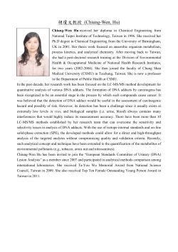


© Copyright 2026