0
2
Dyeing in Computer Graphics
Yuki Morimoto1,3 , Kenji Ono1,2 and Daisaku Arita3
1 RIKEN
2 The
3 ISIT
University of Tokyo
(Institute of Systems, Information Technologies and Nanotechnologies)
Japan
1. Introduction
In this chapter, we introduce a physically-based framework for visual simulation of dyeing.
Since ancient times, dyeing has been employed to color fabrics in both industry and arts and
crafts. Various dyeing techniques are practiced throughout the world, such as wax-resist
dyeing (batik dyeing), hand drawing with dye and paste (Yuzen dyeing), and many other
techniques Polakoff (1971); Yoshiko (2002). Tie-dyeing produces beautiful and unique dyed
patterns. The tie-dyeing process involves performing various geometric operations (folding,
stitching, tying, clamping, pressing, etc.) on a support medium, then dipping the medium
into a dyebath. The process of dipping a cloth into a dyebath is called dip dyeing.
The design of dye patterns is complicated by factors such as dye transfer and cloth
deformation. Professional dyers predict ﬁnal dye patterns based on heuristics; they tap into
years of experience and intimate knowledge of traditional dyeing techniques. Furthermore,
the real dyeing process is time-consuming. For example, clamp resist dyeing requires the
dyer to fashion wooden templates to press the cloth during dyeing. Templates used in this
technique can be very complex. Hand dyed patterns require the dyer’s experience, skill,
and effort, which are combined with the chemical and physical properties of the materials.
This allows the dyer to generate interesting and unique patterns. There are no other painting
techniques that are associated with the deformation of the support medium. In contrast to
hand dyeing, dyeing simulation allow for an inexpensive, fast, and accessible way to create
dyed patterns. We focus on dye transfer phenomenon and woven folded cloth geometry as
important factors to model dyed patterns. Some characteristic features of liquid diffusion on
cloth that are inﬂuenced by weave patterns, such as thin spots and mottles are shown in Figure
1. Also, we adopted some typical models of adsorption isotherms to simply show adsorption.
Figure 2 shows the simulated results obtained using our physics-based dyeing framework and
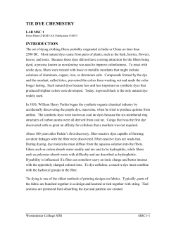
a real dyed pattern. Figure 3 depicts the framework with a corresponding dyeing process.
2. Related work
Non-photorealistic rendering (NPR) methods for painting and transferring pigments on paper
have been developed for watercolor and Chinese ink paintings Bruce (2001); Chu & Tai (2005);
Curtis et al. (1997); Kunii et al. (2001); Wilson (2004). These methods are often based on ﬂuid
www.intechopen.com
16
Natural Dyes
2
Will-be-set-by-IN-TECH
Fig. 1. Some characteristic features of dyeing. (a) thin spots, (b) bleeding ("nijimi" in
Japanese), and (c) mottles.
Our simulated animation results
Real pattern
Magniﬁed images
Fig. 2. Comparisons of our simulated results with a real dyed pattern.
(b) Specify cloth geometry
Press (Stitch)
Fold
(a) Deﬁne weave
(Plain weave)
(c) Supply dyes
(Dip dyeing)
dyer
cloth
dyebath
(A)
(B)
(C)
(D)
(E)
(F)
Fig. 3. The general steps for a real dyeing process (top row Sakakibara (1999)) and our
dyeing framework (bottom row) using the Chinese ﬂower resist technique. (A) The woven
cloth has a plain weave; the blue and yellow cells indicate the warp and the weft. (B) The
unfolded cloth with user speciﬁed fold lines, the red and blue lines indicate ridges and
valleys, and folds in the cloth. (C) The corresponding folded cloth in (B). (D, E) The interfaces
representing user drawings on an unfolded and folded cloth. The gray lines indicate a
user-speciﬁed boundary domain; these will be the dye resist regions. (F) The folded cloth
with the red region indicating the exterior surfaces.
mechanics: Kunii et al. (2001) used Fick’s second law of diffusion to describe water spreading
on dry paper with pigments; Curtis et al. (1997) developed a technique for simulating
watercolor effects; Chu & Tai (2005) presented a real-time drawing algorithm based on the
lattice Boltzmann equation ; and Xu et al. (2007) proposed a generic pigment model based on
rules and formulations derived from studies of adsorption and diffusion in surface chemistry
and the textile industry.
Several studies have also investigated dyeing methods: Wyvill et al. (2004) proposed an
algorithm for rendering cracks in batik that is capable of producing realistic crack patterns
in wax; Shamey (2005) used a numerical simulation of the dyebath to study mass transfer
in a ﬂuid inﬂuenced by dispersion; and Morimoto et al. (2007) used a diffusion model that
www.intechopen.com
173
Dyeing
in Computer
Graphics
Dyeing in Computer
Graphics
includes adsorption to reproduce the details of dyeing characteristics such as thin colored
threads by considering the woven cloth, based on dye physics.
However, the above methods are insufﬁcient for simulating advanced dyeing techniques, such
as tie-dyeing. Previous methods are strictly 2D, and are not designed to handle the folded
3D geometry of the support medium. There is no other simulation method that considers
the folded 3D geometry of the support medium which clearly affects real dyeing results
except for Morimoto et al. (2010). Morimoto et al. (2010) proposed a simulation framework
that simulates dyed patterns produced by folding the cloth. In this chapter, we summerize
these studies.
3. Cloth weave model
We represent the cloth by cells (see Figure 4). We deﬁne two kinds of cells, namely a cloth cell,
and a diffusion cell. In cloth cells, parameters such as the weft or warp, the vertical position
relative to the weave patterns, the size of threads and gaps, and other physical diffusion
factors speciﬁc for each thread are deﬁned. Each cloth cell is subdivided into several diffusion
cells and these diffusion cells are then used to calculate the diffusion.
Initially, cloth cells are deﬁned by the size of the warps and wefts, which can be assigned
arbitrarily. They are then arranged in the cloth at intervals equal to the spacing of gaps.
Two layers are prepared as the weft and warp for cloth cells. Next, a deﬁned weave pattern
determines whether each cloth cell is orientated up or down. Diffusion cells are also arranged
in the cloth size and two layers are formed. Their properties are deﬁned in reference to the
cloth cell in the layer that they are in. Each diffusion cell can have only one of two possible
orientations (parallel to the x and y axes) as the ﬁber’s orientation in its layer. Gravity is
considered to be negligible in our dye transfer model since the dye is usually a colloidal liquid;
this enables us to calculate the diffusion without considering the height in the cloth. There is
thus no necessity to arrange diffusion cells in three-dimensional space, making it is easy to
consider the connection between threads. The effect of height is considered in our model only
for cloth rendering.
gap
warp
weft
cloth cell = diffusion cells
3D weave pattern
warp
side view
Fig. 4. The example of cloth cells with plain weave.
www.intechopen.com
side view
18
Natural Dyes
4
Will-be-set-by-IN-TECH
4. Dye transfer model
Our dye transfer model accounts for the diffusion, adsorption, and supply terms of the dye as
described in an equation (1). The diffusion and adsorption terms describe the dye behavior
based on the second law of Fick (1855) and dyeing physics, respectively. The supply term
enables arbitrary dye distribution for dip dyeing and user drawings.
Let f = f (x, t) ∈ (0, 1] be a dye concentration function with position vector x ∈ ℜ3 and
time parameter t ≥ 0, where t is independent of x. The dyeing model is formulated by the
following evolutionary system of PDEs.
∂ f (x, t)
= div( D (x)∇ f ) + s(x, f ) − a(x, f ),
∂t
(1)
where D (x) is the diffusion coefﬁcient function, div(·) and ∇(·) are the divergence and
gradient operators respectively, and s(·, ·) and a(·, ·) are the source and sink terms that
represent dye supply and adsorption, whereas div( D (x)∇ f ) is the diffusion term. We model
the functions s(·, ·) and a(·, ·) as follows.
αMs (x) if Ms (x) > f (x, t) and Mcd (x) > f (x, t).
s(x, f ) =
0
Otherwise,
a(x, f ) =
β f (x, t) if h(x, t) < ad (x, f ) and Mca (x) > h(x, t).
0
Otherwise,
where α is the user-speciﬁed dye concentration, Ms (x) ∈ [0, 1] is the dye supply map, Mcd (x)
and Mca (x) are the diffusion and adsorption capacity maps, β ∈ [0, 1] is the user-speciﬁed
adsorption rate, and ad (x, f ) is the adsorption capacity according to adsorption isotherms.
The adsorption isotherm depicts the amount of adsorbate on the adsorbent as a function of
its concentration at constant temperature. In this model, we employ the Langmuir adsorption
model Langmuir (1916), which is a saturation curve, to calculate ad (x, f ) in our simulation
based on the model developed by Morimoto et al. Morimoto et al. (2007). The adsorbed dye
concentration h(x, t) ∈ [0, 1] is given by the equation bellow and the evolution of f (x, t) and
h(x, t) as t → ∞ describes the dyeing process.
∂h(x, t)
M (x)
= a(x, f ) cd ,
∂t
Mca (x)
(2)
Designing physically-based diffusion coefﬁcient.
Each diffusion cell has various parameters including its weft layer or warp layer, ﬁber or gap
(i.e., no ﬁber), orientation (either up or down), position, porosity, and tortuosity. Porosity is
deﬁned as the ratio of void volume in a thread ﬁber. Tortuosity denotes the degree of twist, so
that the smaller the value of the tortuosity is, the larger the twist is. We deﬁne three kinds of
tortuosities in our method:
• the twist of the thread (τ1 (x)) deﬁned in each thread
www.intechopen.com
195
Dyeing
in Computer
Graphics
Dyeing in Computer
Graphics
• the position of the thread, including its orientation in the weave pattern (τ2 (x)) determined
by the connection between neighboring diffusion cells, whether they are in the same layer,
whether they contain ﬁbers, and whether their orientation is up or down.
• the different orientations of ﬁbers in neighboring diffusion cells (τ3 (x))
Each of these tortuosities has values in the range (0, 1]. There are ﬁve different conditions for
τ3 (x) which depend on factors such as the layers that neighboring diffusion cells are located
in and their porosity. In Figure 5, colored lines indicate the conditions such as bellow list.
I (blue): Different layer
II (orange): Two ﬁvers are in the same layer, and are connected to each other
perpendicularly
III (purple): Fiber and gap
IV (green): gap and gap
V (red): ﬁver and ﬁver in the same layer
In Figure 5, blue, yellow and white cells represent wefts, warps and gaps. Finally, the
tortuosity of a cell T (x) between diffusion cells is deﬁned as follows:
T (x) = τ1 (x)τ2 (x)τ3 (x)
(3)
The diffusion coefﬁcient is calculated between diffusion cells using the following equation that
is based on the Weisz-Zollinger modelS.-H. (August 1997) in accordance with our deﬁnition
for T (x):
D (x) = D0 p (x) T (x) f 0
(4)
where p is the porosity that can have any value in the range (0, 1], f 0 denotes the
dye concentration in the external solution when equilibrium is achieved and is speciﬁed
arbitrarily. D0 is the diffusion coefﬁcient in free water and is calculated according to the
following equation: Van den (31 Deccember 1994)
√
(5)
D0 = 3.6 76/M
where M denotes the molecular mass of the dye.
(i,j+1,e)
(i-1,j,e)
(i,j,e)
(i+1,j,e)
(i,j-1,e)
Δd
Δd
(i,j,a)
Δd
Fig. 5. Connection between diffusion cells with tortuosity. The third factor in parentheses
indicate the warp / weft layer (a / e).
www.intechopen.com
20
6
Natural Dyes
Will-be-set-by-IN-TECH
Boundary condition.
Let z ∈ B be the boundary domain for dye transfer. We use the Neumann boundary condition
∂ f ( z,t)
∂n ( z )
= b (z) = 0, z ∈ B where n(z) is a unit normal vector of the boundary. In tie-dyeing,
parts of the cloth are pressed together by folding and pressing. We assume that the pressed
region is the boundary domain because no space exists between the pressed cloth parts for
the dye to enter. In our framework, the user speciﬁes B by drawing on both the unfolded and
folded cloth, as shown in Figure 3 (D) and (E), respectively. In the case of the folded cloth,
shown in Figure 3 (E), we project B to all overlapping faces of the folded cloth. Here, the faces
are the polygons of the folded cloth, as shown in the paragraph, Diffusion graph construction.
Press function.
We introduce a press function P (x, c) ∈ [0, 1] as a press effect from dyeing technique. Here c
is a user-speciﬁed cut-off constant describing the domain of inﬂuence of the dye supply and
the capacity maps, and represents the physical parameters. The extent of the pressing effect
and dye permeation depend on the both softness and elasticity of the cloth and on the tying
strength. The press function serves to;
• Limit dye supply (Pressed regions prevent dye diffusion).
• Decrease the dye capacity (Pressed regions have low porosity).
We approximate the magnitude of pressure using the distance ﬁeld dist(x, B) obtained from
the pressed boundary domain B . Note that the press effect only inﬂuences the interior surfaces
of the cloth, as only interior surfaces can press each other.
We deﬁne Ω as the set of exterior surfaces of the tied cloth that are in contact with the dye
and L as the fold lines that the user input to specify the folds. We deﬁne Ω, B , and L as
fold features (Figure 6). We calculate the press function P (x, c) as described in Pseudocode
1. In Pseudocodes 1 and 2, CalcDF () calculates the distance ﬁeld obtained from the fold
feature indicated by the ﬁrst argument, and returns inﬁnity on the fold features indicated by
the second and third arguments. We use m as the number of vertices in the diffusion graph
described in the paragraph "Diffusion graph construction."
Dye supply map.
The dye supply map Ms (x) (Figure 7) describes the distribution of dye sources and sinks on
the cloth, and is applied to the dye supply term in equation (1). In dip dyeing, the dye is
supplied to both the exterior and interior surfaces of the folded cloth. The folded cloth opens
naturally except in pressed regions, allowing liquid to enter the spaces between the folds
(Figure 8). Thus, we assume that Ms (x) is inversely proportional to the distance from Ω, as it
is easier to expose regions that are closer to the liquid dye. Also, the dye supply range depends
on the movement of the cloth in the dyebath. We model this effect by limiting dist(x, Ω) to
a cut-off constant cΩ . Another cut-off constant cB1 limits the inﬂuence of the press function
P (x, cB1 ).
The method used to model the dye supply map Ms (x) is similar to the method used to model
the press function, and is described in Pseudocode 2. In Pseudocode 2, distmax is the max
value of dist(x, Ω) and GaussFilter () is a Gaussian function used to mimic rounded-edge
folding (as opposed to sharp-edge folding) of the cloth.
www.intechopen.com
217
Dyeing
in Computer
Graphics
Dyeing in Computer
Graphics
dist(x, B) ← CalcDF (B , Ω, L)
for i=1 to m do
if dist(i, B) > c then
P (i, c) ← 1.0
else
P (i, c) ← dist(i, B)/c
end if
end for
Pseudocode 1. Press function.
dist(x, Ω) ← CalcDF (Ω, B , L)
for i=1 to m do
dist(i, Ω) ← (distmax − dist(i, Ω))
if dist(i, Ω) > cΩ then
dist(i, Ω) ← P (i, cB1 )
else
dist(i, Ω) ← P (i, cB1 )dist(i, Ω)/cΩ
end if
end for
Ms (x) ← GaussFilter (dist(x, Ω))
Pseudocode 2. Dye supply map.
Capacity maps.
The capacity maps indicate the dye capacities in a cloth; they deﬁne the spaces that dyes can
occupy. We ﬁrst calculate the basic capacities from a ﬁbre porosity parameter Morimoto et al.
(2007). The cut-off constant cB2 limits the press function P (x, cB2 ) used here. We then multiply
these capacities by the press function to obtain the capacity maps Mcd (x) and Mca (x) as
followings (see Figure 9).
Mcd (x) = Vd (x) P (x, cB2 ),
Mca (x) = Va (x) P (x, cB2 ),
(6)
The basic capacity of the dye absorption in the diffusion cell Va (x) is determined by the ratio
of ﬁber in the diffusion cell according to the following expression:
Va (x) = 1 − p (x)
(7)
Also, the maximum amount of dye adsorption (ﬁxing dye) into ﬁbers (ad (x, f )) is calculated
each time step by adsorption isotherm based on the dyeing theories used in our model
Langmuir (1916), Vickerstaff (1954). Figure 13 shows representative behavior of these typical
adsorption isotherms. If we use the Freundlich equation (Figure 13 (b")) in our system, we can
deﬁne ad (x, f ) as:
ad = k f b
(8)
where k is a constant, and B is a constant that lies in the range (0.1, 1). If b = 1, eq 8 become a
linear equilibrium as shown in Figure 13 (a"). If we use the Langmuir equation (Figure 13 (c"))
www.intechopen.com
22
Natural Dyes
8
Will-be-set-by-IN-TECH
Cut-off
Normalize/
/
Press function
P (x, cB1 )
Fold features Distance ﬁeld
dist(x, B)
Fig. 6. An example for calculating the press function P (x, cB1 ) for the Chinese ﬂower resist.
In the fold features, the exterior surface Ω, pressed boundary domain B , and the fold lines L
are shown by red, gray, and blue colors.
Invert,
cut-off by
cΩ ,
/
Multiply
by
P ( x, cB1 )
Smoothing
/
/
normalize
Distance ﬁeld
dist(x, Ω)
Dye supply map
Ms ( x )
Fig. 7. An illustration of the dye supply map Ms (x) for the Chinese ﬂower resist.
Fig. 8. Photographs of real dip dyeing. The left shows a folded cloth pressed between two
wooden plates. The right shows folded cloths that have opened naturally in liquid.
Basic capacity Press function Capacity map
P (x, cB2 )
Vd
Mcd (x)
Fig. 9. Illustration for our diffusion capacity map Mcd (x) calculated by taking the product of
the basic capacity and P (x, cB2 ).
www.intechopen.com
239
Dyeing
in Computer
Graphics
Dyeing in Computer
Graphics
in our model, we can deﬁned ad (x, f ) as:
ad (x, f ) =
Mcd (x)K L f
1 + KL f
(9)
where K L is the equilibrium constant. The resulting images are shown in Figure 12 and
are calculated using these adsorption isotherms. The parameter b (z) prevents dyeing in
the pressed area of the cloth and is used to represent the dyeing patterns of certain dyeing
techniques. Curtis et al. (1997) used a similar method in which the paper affects ﬂuid ﬂow
to some extent for watercolor and by doing so generates patterns. But the effect of this
phenomenon is not as pronounced as that of dyeing patterns. In our method, we use the
amount of dye that is not absorbed by the ﬁber to calculate the total amount of dye in the
diffusion cell. The basic diffusion capacity Vd (x) is calculated as bellow,
Vd (x) = p (x)(1 − b (z)),
(10)
Diffusion graph construction.
We construct multiple two-layered cells from the two-layered cellular cloth model by
cloth-folding operations. The diffusion graph G is a weighted 3D graph with vertices v i , edges,
and weights wij where i, j = 1, 2, .., m. The vertex v i in the diffusion graph G is given by the
cell center.
We apply the ORIPA algorithm Mitani (2008), which generates the folded paper geometry
from the development diagram, to the user-speciﬁed fold lines on a rectangular cloth. The
fold lines divide the cloth into a set of faces as shown in Figure 3 (B). The ORIPA algorithm
generates the corresponding vertex positions of faces on the folded and unfolded cloths and
the overlapping relation between every two faces as shown in Figure 3 (C). We apply ID
rendering to the faces to obtain the overlapping relation for multiple two-layered cells. We
then determine the contact areas between cells in the folded cloth, and construct the diffusion
graph G by connecting all vertices v i to vertices v j in the adjacent contact cell by edges, as
illustrated in Figure 10.
Graph
(a) An illustration for the
multiple two-layered cloth
model.
Vj
Vi
(b) A graph in dot square in (a). (c) Contact cells.
Fig. 10. Graph construction from folded geometry of woven cloth. The bold line in (a)
represents a fold line. The gray points in (c) are contact cell vertices v j of the target cell vertex
vi .
www.intechopen.com
24
Natural Dyes
10
Will-be-set-by-IN-TECH
Fig. 11. Computer generated dye stains with various parameters including T (x), p (x),
weave, etc. Total number of time steps is 5000.
Discretization in diffusion graph.
The ﬁnite difference approximation of the diffusion term of equation (1) at vertex v i of G is
given by
divD (x)∇ f ≈
∑
j∈ N ( i)
wij
f (v j , t) − f (v i , t)
| v j − v i |2
,
(11)
where wij = Dij Aij , N (i ) is an index set of vertices adjacent to v i in G , and Dij and Aij are
the diffusion coefﬁcient and the contact area ratio between vertices v i and v j , respectively
(Figure 10). We calculate the distance between v i and v j from cell sizes, δx, δy, δz, and deﬁne
Dij = ( D (v i ) + D (v j ))/2 between vertices connected by folding.
The following semi-implicit scheme gives our discrete formulation of equation (1):
( I − (δt) L )fn+1 = fn + δt(sn − an ),
(12)
which is solved using the SOR solver Press et al. (1992), where I is the identity matrix, δt is
the discrete time-step parameter, n is the time step, and
fn = { f (v1 , n ), f (v2 , n ), .., f (v m , n )},
sn = {s(v1 , f (v1 , n )), s(v2 , f (v2 , n )), .., s(v m , f (v m , n ))},
an = { a(v1 , f (v1 , n )), a(v2 , f (v2 , n )), .., a(v m , f (v m , n ))},
L is the mxm graph Laplacian matrix Chung (1997) of G . The element l ij of L is given by
l ij =
wij /| v j − v i |2 if i = j,
− ∑ j∈ N ( i) lij Otherwise.
(13)
We then simply apply the forward Euler scheme to equation (2):
h(v i , n + 1) = h(v i , n ) + δta(v i , f (v i , n ))
Mcd (v i )
Mca (v i )
(14)
The diffused and adsorbed dye amounts at v i are given by f (v i , n ) Mcd (v i ) and
h(v i , n ) Mca (v i ), respectively. The dye transfer calculation stops when the evolution of
n
n−1 | /m ≤ .
equation (1)converges to ∑m
i =1 | f ( v i , n ) − f ( v i , n )
www.intechopen.com
Dyeing
in Computer
Graphics
Dyeing in Computer
Graphics
25
11
Fig. 12. Comparison of simulations with some adsorption isotherms. Total numbers of time
steps is 50000.
Fig. 13. Behavior of some typical adsorption isotherms.
5. Result
For visualizations of the dyed cloth, we render the images by taking the product of the sum
of dye (transferred and adsorbed) and its corresponding weft and warp texture.
Physically-based model
The results of our simulation are shown in Figs. 11, 12. Figure 11 (d) shows mottles similar to
those in Figure 1 (c). This shows that mottles are formed with not just when the value of τ3 I (x)
is small but they are also produced by the two-layered model. Figures 11 (f) and (g) show the
results for random p (x), while Figure 11 (e) shows the result for random τ1 (x). Some thin
colored threads can clearly be seen in Figure 11 (f). We ﬁnd that p (x) has more effect on the
ﬁnal appearance than τ1 (x). Figure 11 (b) shows the result obtained when a high absorption
coefﬁcient is used; in this result, the initial dyeing area seems to contain a lot of dye.
Figure 12 shows results calculated using some adsorption isotherms as shown in Figure 13.
(a) and (b) are the result obtained using the Freundlich model (eq 8) where b = 1, k = 1 and
b = 0.3, k = 1. (c) is the result obtained using the Langmuir model (eq 9). (a’), (b’) and (c’)
show only the absorbed dye densities of (a), (b) and (c), respectively. In this comparison, we
can observe the effect of the kind of adsorption isotherm has on the results obtained.
Folded cloth geometry
Figure 14 shows real dyed cloth and our simulated results for a selection of tie-dyeing
techniques. The dyeing results are evaluated by examining the color gradation, which stems
from cloth geometry. Our framework is capable of generating heterogeneous dyeing results by
www.intechopen.com
26
Natural Dyes
12
Will-be-set-by-IN-TECH
visualizing the dye transferring process. While we cannot perform a direct comparison of our
simulated results to real results, as we are unable to precisely match the initial conditions or
account for other detailed factors in the dyeing process, our simulated results (a, b) corrspond
well with real dyeing results (c).
(a) n = 2700
(b) n = 7693
(c)
Seikaiha pattern
(a) n = 300
(b) n = 3968
(c)
Kumo shibori
(a) n = 500
(b) n = 1567
(c)
Itajime
(g)
(f)
(h)
Seikaiha pattern.
(f)
(g)
(h)
Kumo shibori.
(d)
(e)
(d)
(e)
(d)
(e)
(f)
(g)
Itajime
(h)
Fig. 14. Various tie-dyeing results and their corresponding conditions. (a) Our simulated
results. (b) Our converged simulated results. (c) Real tie-dyeing results Sakakibara (1999). (d)
Tie-dyeing techniques. (e) Folded cloths with user-speciﬁed boundary domains. (f) Fold
features. (g) Dye supply maps Ms (x). (h) Dye capacity maps Mcd (x). In (f), (g), and (h), the
top and bottom images indicate the top and bottom layers of the cloth model, respectively.
The thin gray regions in the Seikaiha pattern (e) indicate regions that were covered with a
plastic sheet to prevent dye supply on them; they are not the boundary domain. n is the
number of time steps.
www.intechopen.com
Dyeing
in Computer
Graphics
Dyeing in Computer
Graphics
27
13
6. Conclusion
In this article, we introduced physically-based dyeing simulation frameworks.
The
framework is able to generate a wide range of dyed patterns produced using a folded woven
cloth, which are difﬁcult to produce by conventional methods.
It is important to create real-world dyed stuffs using this system as an user study. However,
these systems are not enough to simulate complex dyed patterns intuitively. For example, an
interface for modeling dyeing techniques such as complex cloth geometries and coloring are
important but they are not achieved. Other future work to simulate dyed patterns by PC is
enriching physical simulation of dyeing. In the CG dyeing methods we introduced, there is
no advection and color mixing. These factors make the dyeing system attractive and useful
more.
After these future work achieved, practical problems of dyeing can be addressed. The
problems include archiving and restoring traditional dyeing techniques, designing graphics of
dyeing, education of the dyeing culture, etc. One of our important goal is that the real-world
dyeing would be raised through these approaches. The dyeing frameworks in computer
graphics should be used to enhance social interests in dyeing and enrich understanding but
replace traditional real-world dyeing work. People can use the CG dyeing method for a wide
range of aims. The methods include some factors of physics and design. In the future, visual
simulation of dyeing would be able to develop as a theme between some scientic areas and be
utilized widely.
7. References
Bruce Gooch, A. G. (2001). Non-Photorealistic Rendering, A K Peters Ltd.
Chu, N. S.-H. & Tai, C.-L. (2005). Moxi: real-time ink dispersion in absorbent paper, ACM
Trans. Graph. 24(3): 504–511.
Chung, F. R. K. (1997). Spectral Graph Theory, American Mathematical Society. CBMS, Regional
Conference Series in Mathematics, Number 92.
Curtis, C. J., Anderson, S. E., Seims, J. E., Fleischer, K. W. & Salesin, D. H.
(1997). Computer-generated watercolor, Computer Graphics 31(Annual Conference
Series): 421–430. URL: citeseer.ist.psu.edu/article/curtis97computergenerated.htm
Fick, A. (1855). On liquid diffusion, Jour. Sci. 10: 31–39.
Kunii, T. L., Nosovskij, G. V. & Vecherinin, V. L. (2001). Two-dimensional diffusion model for
diffuse ink painting, Int. J. of Shape Modeling 7(1): 45–58.
Langmuir, I. (1916). The constitution and fundamental properties of solids and liquids. part i.
solids., Journal of the American Chemical Society 38: 2221–2295.
Mitani, J. (2008). The folded shape restoration and the CG display of origami from the crease
pattern, 13th international Conference on Geometry and Graphics.
Morimoto, Y., Tanaka, M., Tsuruno, R. & Tomimatsu, K. (2007). Visualization of dyeing based
on diffusion and adsorption theories, Proc. of Pacific Graphics, IEEE Computer Society,
pp. 57–64.
Morimoto, Y., & Ono, K. (2010). Computer-Generated Tie-Dyeing Using a 3D Diffusion Graph,
In Advances in VisualComputing (6th International Symposium on Computer Vision - ISVC
2010 (Oral presentation)), Lecture Notes in Computer Science, Springer, volume 6453,
pages 707–718.
www.intechopen.com
28
14
Natural Dyes
Will-be-set-by-IN-TECH
Polakoff, C. (1971). The art of tie and dye in africa, African Arts, African Studies Centre 4(3).
Press, W. H., Teukolsky, S. A., Vetterling, W. T. & Flannery, B. P. (1992). Numerical recipes in C
(2nd ed.): the art of scientific computing, Cambridge University Press.
S.-H., B. (August 1997). Diffusion/adsorption behaviour of reactive dyes in cellulose, Dyes and
Pigments 34: 321–340(20). URL: http://www.ingentaconnect.com/content/els/01437208/
1997/00000034/00000004/art00080
Sakakibara, A. (1999). Nihon Dento Shibori no Waza (Japanese Tie-dyeing Techniques), Shiko Sha
(in Japanese).
Shamey, R., Zhao, X., Wardman, R. H. (2005). Numerical simulation of dyebath and the
inﬂuence of dispersion factor on dye transport, Proc. of the 37th conf. on Winter
simulation, Winter Simulation Conference, pp. 2395–2399.
Van den, B. R. (31 Deccember 1994). Human exposure to soil contamination: a qualitative and
quantitative analysis towards proposals for human toxicological intervention values
(partly revised edition), RIVM Rapport 725201011: 321–340(20).
URL: http://hdl.handle.net/10029/10459
Vickerstaff, T. (1954). The Physical Chemistry of Dyeing, Oliver and Boyd, London.
Yoshiko, W. I. (2002). Memory on Cloth:Shibori Now, Kodansha International.
Wilson, B., Ma, K.-L. (2004). Rendering complexity in computer-generated pen-and-ink
illustrations. Proc. of Int. Symp. on NPAR, ACM, pp. 129–137.
Wyvill, B., van Overveld, K. & Carpendale, S. (2004). Rendering cracks in batik, NPAR
’04: Proceedings of the 3rd international symposium on Non-photorealistic animation and
rendering, ACM Press, New York, NY, USA, pp. 61–149.
S. Xu, H. Tan, X. Jiao, F.C.M. Lau, & Y. Pan (2007). A Generic Pigment Model for Digital
Painting, Computer Graphics Forum (EG 2007), Vol. 26, pp. 609–618.
www.intechopen.com
Natural Dyes
Edited by Dr. Emriye Akcakoca Kumbasar
ISBN 978-953-307-783-3
Hard cover, 124 pages
Publisher InTech
Published online 14, November, 2011
Published in print edition November, 2011
Textile materials without colorants cannot be imagined and according to archaeological evidence dyeing has
been widely used for over 5000 years. With the development of chemical industry all finishing processes of
textile materials are developing continuously and, ecological and sustainable production methods are very
important nowadays. In this book you can be find the results about the latest researches on natural dyeing.
How to reference
In order to correctly reference this scholarly work, feel free to copy and paste the following:
Yuki Morimoto, Kenji Ono and Daisaku Arita (2011). Dyeing in Computer Graphics, Natural Dyes, Dr. Emriye
Akcakoca Kumbasar (Ed.), ISBN: 978-953-307-783-3, InTech, Available from:
http://www.intechopen.com/books/natural-dyes/dyeing-in-computer-graphics
InTech Europe
University Campus STeP Ri
Slavka Krautzeka 83/A
51000 Rijeka, Croatia
Phone: +385 (51) 770 447
Fax: +385 (51) 686 166
www.intechopen.com
InTech China
Unit 405, Office Block, Hotel Equatorial Shanghai
No.65, Yan An Road (West), Shanghai, 200040, China
Phone: +86-21-62489820
Fax: +86-21-62489821