CONTENTS
1
INTRODUCTION
Lecture 4: Nonlinear accessibility, controllability, and observability
Jorge Cort´es
May 12, 2015
Abstract
In this lecture, we move away from the emphasis of the previous lectures on stabilization and tracking,
and focus instead on investigating controllability and observability of nonlinear control systems affine in
the inputs. Throughout the lecture, we try to understand the set of states that can be reached and can be
observed by using open-loop inputs. The treatment corresponds to selected parts from Chapter 3 in [1],
Chapter 4 in [2], and Chapter 2 in [3].
Contents
1 Introduction
1
2 Accessibility and controllability
2
2.1
Accessibility and strong accessibility . . . . . . . . . . . . . . . . . . . . . . . . . . . . . . . .
2
2.2
Controllability . . . . . . . . . . . . . . . . . . . . . . . . . . . . . . . . . . . . . . . . . . . .
3
3 The linear controllability test
3
4 Nonlinear tests for (strong) accessibility
4
4.1
4.2
Nonlinear tests for accessibility . . . . . . . . . . . . . . . . . . . . . . . . . . . . . . . . . . .
4
4.1.1
Accessibility and controllability of linear systems from the origin . . . . . . . . . . . .
7
Nonlinear tests for strong accessibility . . . . . . . . . . . . . . . . . . . . . . . . . . . . . . .
7
5 Nonlinear tests for controllability
9
6 Observability
1
11
Introduction
Consider the multiple-input system on Rn
x˙ = f (x) +
m
X
ui gi (x)
(1)
i=1
1
MAE281b – Nonlinear Control
c 2008-2015 by Jorge Cort´
Copyright es. Permission is granted to copy, distribute and modify this file, provided that the
original source is acknowledged.
2 ACCESSIBILITY AND CONTROLLABILITY
where u = (u1 , . . . , um ) ∈ U ⊂ Rm . The first question we answer in this lecture is: given an initial x0 ∈ Rn ,
what set of points are reachable from x0 in finite time by using open-loop inputs that take values in U ?
Consider the multiple-input-multiple-output system on Rn
x˙ = f (x) +
m
X
ui gi (x)
(2a)
i=1
1 ≤ j ≤ p,
yj = hj (x),
(2b)
where hi : Rn → R. The second question we answer in this lecture is: can the state x0 ∈ Rn be distinguished
(at the output level) from its neighbors by using system trajectories that remain close to x0 and are generated
with open-loop inputs that take values in U ?
2
Accessibility and controllability
For linear systems, x˙ = Ax + Bu, x ∈ Rn , u ∈ Rm , the celebrated Kalman rank condition
rank(B|AB|A2 B| . . . |An−1 B) = n
fully characterizes when the system is (globally) controllable (from any point).
Our objective here is to come up with similar tests for nonlinear systems. Let us start by making precise the
notions of accessibility and controllability.
2.1
Accessibility and strong accessibility
For the system (1), let RV (x0 , T ) be the reachable set from x0 in time exactly T > 0 following trajectories
that remain in the neighborhood V of x0 for time t ≤ T . In other words,
RV (x0 , T ) = {x ∈ Rn | ∃u : [0, T ] → U such that x(0) = x0 , x(t) ∈ V, 0 ≤ t ≤ T, x(T ) = x}
This is the set of points reachable from x0 in time exactly T . Next, define the set of points reachable from
x0 in time up to T ,
[
RV (x0 , ≤ T ) =
RV (x0 , t)
t≤T
Definition 2.1 (Local accessibility) The system (1) is small-time locally accessible from x0 if for any
neighborhood V of x0 and T > 0, the set RV (x0 , ≤ T ) contains a non-empty open set. If this holds for
any x0 , then the system is called small-time locally accessible.
When one looks at the points that can be reached not within time T , but exactly at time T , a stronger
version of accessibility arises.
Definition 2.2 (Local strong accessibility) The system (1) is small-time locally strongly accessible from
x0 if for any neighborhood V of x0 , the set RV (x0 , T ) contains a non-empty open set for T small enough. If
this holds for any x0 , then the system is called small-time locally strongly accessible.
Clearly, small-time local strong accessibility from x0 implies small-time local accessibility from x0 . The
converse is in general not true. As an example, the linear control system x˙ = x (with B = 0) on R is
small-time locally accessible from any x 6= 0, but is not small-time strongly accessible.
2
MAE281b – Nonlinear Control
c 2008-2015 by Jorge Cort´
Copyright es. Permission is granted to copy, distribute and modify this file, provided that the
original source is acknowledged.
2.2
2.2
Controllability
3 THE LINEAR CONTROLLABILITY TEST
Controllability
Here, we distinguish between local and global controllability.
Definition 2.3 (Local controllability) The system (1) is small-time locally controllable from x0 if for
any neighborhood V of x0 , the set RV (x0 , ≤ T ) is a neighborhood of x0 for each T small enough. If this holds
for any x0 , then the system is called small-time locally controllable.
Clearly, small-time local controllability implies small-time local accessibility. It turns out that, for a large
class of systems (including Euclidean spaces), small-time local controllability implies small-time local strong
accessibility. More specifically, this result is true for state spaces that are manifolds whose fundamental group
has no elements of infinite order. A formal proof of this statement can be found in [4].
The converse are not true. Counterexamples are shown later in Examples 4.6 and 4.13. If the control system
is driftless, i.e., f = 0, then accessibility and controllability are equivalent.
Definition 2.4 (Global controllability) The system (1) is globally controllable from x1 if for any x2 ∈
Rn , there exists T > 0 and u : [0, T ] → U such that the solution of (1) starting at x1 at time 0 with control
u satisfies x(T ) = x2 .
Note that in the notion of global controllability, there is no requirement of the trajectories of the system
remaining close to the starting point, i.e., excursions are allowed (which makes sense because it is global!).
3
The linear controllability test
What about linearizing the nonlinear system and studying the controllability properties of its linearization?
Will that reveal information about the controllability of the nonlinear system? The following result states
that this is a good approach.
Proposition 3.1 (Linear controllability) Consider (1) and let x0 ∈ Rn with f (x0 ) = 0. Assume U
contains a neighborhood of 0. Suppose the linearization at x0 and u = 0,
z˙ =
m
X
∂f
vj gj (x0 ),
(x0 )z +
∂x
i=1
z ∈ Rn ,
v ∈ Rm ,
is controllable (in the sense of a linear system). Then, the system is small-time locally controllable from x0 .
This result is a step in the good direction. However, linearization is often not enough. A nonlinear system
can be controllable while its linearization is not.
Example 3.2 (Unicycle) Consider the unicycle dynamics
x˙ = u cos θ
y˙ = u sin θ
θ˙ = v
Note that any state is an unforced equilibrium because the system is dritfless. The linearization at (x∗ , y∗ , θ∗ )
is


cos θ∗ 0 u
z˙ =  sin θ∗ 0
v
0
1
3
MAE281b – Nonlinear Control
c 2008-2015 by Jorge Cort´
Copyright es. Permission is granted to copy, distribute and modify this file, provided that the
original source is acknowledged.
4
NONLINEAR TESTS FOR (STRONG) ACCESSIBILITY
which clearly is not controllable (A = 0 and hence the Kalman rank condition is not satisfied). However,
most kids know by experience that the unicycle is actually globally controllable!
•
What we have seen in Example 3.2 (the nonlinear system being controllable while its linearization is not) is
quite common in nonlinear systems.
4
Nonlinear tests for (strong) accessibility
In this section, we provide nonlinear tests for local accessibility and local strong accessibility.
4.1
Nonlinear tests for accessibility
Let us again look at the original system (1). In what directions can we steer the system from x0 ∈ Rn , i.e.,
what points can be reached in arbitrarily small time? Consider the simpler system
x˙ = u1 g1 (x) + u2 g2 (x).
(3)
Clearly, we can steer the system in the direction of g1 and g2 . But can we steer the system in more directions?
Yes! We saw something along these lines when we first introduced the notion of Lie bracket in the notes on
“Feedback Linearization.” For instance, one can establish the following result.
Lemma 4.1 Let h > 0, and consider the control function

0≤t<h

(1, 0),

(0, 1),
h ≤ t < 2h
u(t) =
(−1, 0), 2h ≤ t < 3h



(0, −1), 3h ≤ t < 4h
(4)
Then the solution of (3) under the input (4) starting at x0 satisfies
x(4h) = x0 + h2 [g1 , g2 ](x0 ) + O(h3 ).
Example 4.2 (Unicycle revisited) For the unicycle case, cf. Example 3.2, the dynamics is of the form (3)
with
 


0
cos θ
g 2 = 0
g1 =  sin θ  ,
1
0
The Lie bracket of g1 and g2 is given by


sin θ
[g1 , g2 ] = − − cos θ
0
which corresponds to motion along the sideways direction!
•
Lemma 4.1 is only the beginning. By choosing more elaborate switching sequences than (4), it is also
possible to move in directions given by higher-order Lie brackets such as [g2 , [g1 , g2 ]] or [[g1 , g2 ], [g2 , [g1 , g2 ]]].
Furthermore, in case there is a drift term f in the equations, then we also have to consider Lie brackets
4
MAE281b – Nonlinear Control
c 2008-2015 by Jorge Cort´
Copyright es. Permission is granted to copy, distribute and modify this file, provided that the
original source is acknowledged.
4.1
Nonlinear tests for accessibility
4
NONLINEAR TESTS FOR (STRONG) ACCESSIBILITY
involving f . (In general, we cannot move back and forth along f , but by making the right switches, we can
move along directions that involve brackets of f and the inputs g1 , . . . , gm ).
Inspired by the previous discussion, let us define the accessibility distribution by
C(x) = span{X(x) | X is a linear combination of repeated Lie brackets of the form
[Xk , [Xk−1 , . . . , [X2 , X1 ] . . . ]] with Xi ∈ {f, g1 , . . . , gm } and k = 1, 2, . . . }
Exercise 4.3 Can you show that C is involutive?
The following result relates the notions of accessibility distribution and local accessibility.
Theorem 4.4 (Accessibility test) Consider (1) and let x0 ∈ Rn . Assume
dim C(x0 ) = n.
Then the system is small-time locally accessible from x0 .
The condition of Theorem 4.4 is called the accessibility rank condition (and also Chow’s theorem).
Corollary 4.5 If dim C(x) = n for all x ∈ Rn , the system is small-time locally accessible.
As we mentioned in Section 2, accessibility is not the same as controllability. The next example shows that
they are different notions.
Example 4.6 Consider the system
x˙ 1 = x22
x˙ 2 = u
We may rewrite the system as
x˙ =
x22
0
0
+
u = f (x) + g(x)u
1
One can compute the Lie brackets
[f, g] = −
2x2
,
0
[[f, g], g] =
2
0
Therefore, dim C(x) = 2 for all x ∈ R2 , and the system is small-time locally accessible. However, since
x˙ 1 = x22 ≥ 0, the x1 coordinate always grows if we are not at the x2 -axis. So the system is not small-time
locally controllable! This is precisely because the drift steers the system to the right.
•
The sufficient condition for accessibility in Theorem 4.4 and Corollary 4.5 is also “almost” necessary. More
precisely, we have the following result (recall that a set A ⊂ X is dense in a topological space X if A = X).
Proposition 4.7 If (1) is small-time locally accessible for all x ∈ Rn , then dim C(x) = n on an open and
dense subset of Rn .
In general, one needs to proceed carefully with the computation of C because it is not known a priori how
many Lie brackets of the vector fields need to be done until the accessibility distribution has been fully
computed. The next two remarks offer a few observations that can help simplify this task.
5
MAE281b – Nonlinear Control
c 2008-2015 by Jorge Cort´
Copyright es. Permission is granted to copy, distribute and modify this file, provided that the
original source is acknowledged.
4.1
Nonlinear tests for accessibility
4
NONLINEAR TESTS FOR (STRONG) ACCESSIBILITY
Remark 4.8 (Homogeneous vector fields) Let ∆ : Rn → Rn the dilation vector field given by ∆(x) = x.
A vector field X : Rn → Rn is homogeneous of degree d ∈ N ∪ {0} if [∆, X] = (d − 1)X. Note that this
is equivalent to saying that the components of X are homogeneous polynomials of degree d in the variables
x1 , . . . , xn . To see this, compute
[∆, X] =
∂∆
∂X
∂X
∆−
X=
∆−X
∂x
∂x
∂x
Then, the definition of homogeneous vector field implies that
tions are the following:
∂X
∂x (x)x
= d · X(x). Three interesting observa-
(i) The Lie bracket of two homogeneous vector fields, say X1 of degree d1 and X2 of degree d2 , is also
homogeneous, of degree d1 + d2 − 1 (use the Jacobi identity to provide an elegant proof of this fact!).
(ii) Homogeneous vector fields of zero degree are constants and there are no homogeneous vector fields of
negative degree (other than the trivial one, identically zero). Therefore, with the notation of the above
item, if d1 + d2 − 1 < 0, then [X1 , X2 ] = 0.
(iii) The above observations are also valid, with the appropriate modifications, for vector fields that are not
homogeneous, but are a linear combination of homogeneous vector fields of different degrees because of
the linearity of the Lie bracket.
•
Remark 4.9 (Phillip Hall basis) The systematic computation that must be performed to compute the
accessibility distribution can be ‘organized’ by means of the notion of Phillip Hall basis. The idea is to
start with the vector fields f, g1 , . . . , gm , and iteratively generate the minimal number of new vector fields
using Lie brackets. We emphasize the term minimal because of the following observation. Say that we have
already computed [X2 , [X1 , X3 ]] and [X3 , [X1 , X2 ]] for some vector fields X1 , X2 , X3 . Then, there is no point
in computing [X1 , [X2 , X3 ]], because the Jacobi identity states that
[X1 , [X2 , X3 ]] = −[X2 , [X3 , X1 ]] − [X3 , [X1 , X2 ]].
The notion of Phillip Hall basis is a formalization of this observation, that we tackle next. Given X1 , . . . , Xm ,
the order d of a Lie product is defined recursively as follows. Let d(Xi ) = 1. For any Lie product [φ1 , φ2 ], let
d([φ1 , φ2 ]) = d(φ1 ) + d(φ2 )
The order essentially corresponds to the number of basis vector fields that appear in the Lie bracket. A
Phillip Hall basis is a sequence {φ1 , φ2 , . . . } of Lie products for which
(i) the vector fields X1 , . . . , Xm are the first m elements
(ii) if d(φi ) < d(φj ), then i < j
(iii) [φi , φj ] belongs to the basis if and only if
(a) φi , φj belong to the basis and i < j, and
(b) either φj = Xi for some i or φj = [φl , φr ] for some φl , φr in the basis with l ≤ i
This procedure results in a basis for the Lie algebra generated by X1 , . . . , Xm .
For instance, up to order 3, the elements of the basis for X1 , X2 , X3 are
X1
[X1 , X2 ]
[X1 , [X1 , X2 ]]
[X2 , [X2 , X3 ]]
X2
[X1 , X3 ]
[X1 , [X1 , X3 ]]
[X3 , [X1 , X2 ]]
X3
[X2 , X3 ]
[X2 , [X1 , X2 ]]
[X3 , [X1 , X3 ]]
[X2 , [X1 , X3 ]]
[X3 , [X2 , X3 ]]
Note that the only Lie bracket that has been automatically eliminated up to this order is [X1 , [X2 , X3 ]].
6
MAE281b – Nonlinear Control
c 2008-2015 by Jorge Cort´
Copyright es. Permission is granted to copy, distribute and modify this file, provided that the
original source is acknowledged.
•
4.2
Nonlinear tests for strong accessibility 4
4.1.1
NONLINEAR TESTS FOR (STRONG) ACCESSIBILITY
Accessibility and controllability of linear systems from the origin
For a linear system x˙ = Ax + Bu, accessibility from the origin is equivalent to controllability from the origin.
This fact can be deduced from the explicit expression of the solution given an open-loop control
Z t
At
e−Aτ Bu(τ )dτ + x0 .
(5)
x(t) = e
0
Since we start from 0, we have x0 = 0. From (5), we deduce the following basic facts:
(i) if the system attains in time T a point x∗ , it can attain any point in span{x∗ } in time T .
This is because if the system attains a point x∗ at time T with control u(t), it can also attain the point αx∗
in time T with control αu(t), for any α 6= 0. Additionally,
(ii) if the system attains in time T a point x1 with input u1 (t) and a point x2 with input u2 (t), then it can
attain any point in span{x1 , x2 } in time T .
This is because the system can attain the point α1 x1 +α2 x2 in time T with control α1 u1 (t)+α2 u2 (t). Finally,
we also have
(iii) if the system attains in time T a point x∗ with open-loop input u(t), it can attain also attain x∗ in
time βT , with β > 0.
To show this, consider the open-loop input
v(t) =
1 T −1 T A(T − βt )(1−β) t .
(B B) B e
Bu
β
β
From the above discussion, one can now establish the following result.
Lemma 4.10 A linear system is locally accessible from 0 if and only if it is locally controllable from 0.
Clearly, controllability implies accessibility by definition. The other implication follows from a careful application of the above facts. Since the set of reachable points is open, we can find n linearly independent vectors
x1 , . . . , xn that can be reached in up to time T > 0, for T small enough. These points might be reached
at different times, say t1 , . . . , tn . However, after an appropriate re-scaling, we know from (iii) that we can
assume that the are all attained at the same time, say t∗ . The application of (ii) now guarantees that the
system can attain any state starting from 0.
4.2
Nonlinear tests for strong accessibility
What if we apply our criteria for accessibility to a linear system? Take
x˙ = Ax + Bu = Ax +
m
X
bi u i
i=1
where B = (b1 | . . . |bm ). Clearly [bi , bj ] = 0. On the other hand, we have
[Ax, bi ] = −Abi .
7
MAE281b – Nonlinear Control
c 2008-2015 by Jorge Cort´
Copyright es. Permission is granted to copy, distribute and modify this file, provided that the
original source is acknowledged.
4.2
Nonlinear tests for strong accessibility 4
NONLINEAR TESTS FOR (STRONG) ACCESSIBILITY
Moreover,
[[Ax, bi ], bj ] = 0
[[Ax, bi ], [Ax, bj ]] = 0
[[Ax, bi ], Ax] = −A2 bi
..
.
Therefore, the accessibility distribution C is spanned by the constant vector fields bi , Abi , A2 bi , . . . , for
i = 1, . . . , m, together with Ax.
Recall that by Cayley-Hamilton, we know that Ak bi , for k ≥ n, is a linear combination of bi , Abi , . . . , An−1 bi .
This leads us to conclude that
C(x) = Im(B, AB, A2 B, . . . , An−1 B) + span{Ax}.
From this we observe the following:
(i) At x0 = 0, we recover the Kalman rank condition
(ii) If we did not know anything about linear systems, then we could conclude that if the Kalman rank
condition is satisfied, then the system is small-time locally accessible. (Actually, from Lemma 4.10, we
can deduce that if the Kalman rank condition is satisfied, then the system is small-time accessible from
zero, and therefore it is controllable from zero. Can you deduce from this that the system is controllable
starting from any point? )
(iii) Notice that span{Ax} is not present in the Kalman rank condition. Furthermore, for linear systems,
we know that not only RV (x0 , ≤ T ) but also RV (x0 , T ) contains an open set.
From the observations above, it is clear there is some more juice we can squeeze out of our discussion. Starting
from a point different than the origin, the system might be locally accessible while still not satisfying the
Kalman rank condition. And (iii) tells us that if the system is locally accessible, it can actually reach an
open set of points not within, but at a specific time.
Define then the strong accessibility distribution,
C0 (x) = span{X(x) | X is a linear combination of repeated Lie brackets of the form
[Xk , [Xk−1 , . . . , [X1 , gj ] . . . ]] with j = 1, . . . , m, Xi ∈ {f, g1 , . . . , gm } and k = 0, 1, 2, . . . }
Note that, in general, C0 (x) ⊂ C(x). We are now ready to state the following result.
Theorem 4.11 (Strong accessibility test) Consider the system (1). Then the following holds:
(i) If dim C0 (x0 ) = n, then the system is small-time locally strongly accessible from x0
(ii) If the system is small-time locally strongly accessible, then dim C0 (x) = n on an open and dense set of
Rn .
Because of the inclusion C0 (x) ⊂ C(x), we see that it is more difficult to satisfy the strong accessibility
test in Theorem 4.11 than it is to satisfy the accessibility test in Theorem 4.4. This makes sense, as strong
accessibility is a stronger notion than accessibility.
Exercise 4.12 Compute the strong accessibility distribution for a linear system x˙ = Ax + Bu. Use the
result to deduce that strong accessibility and controllability are equivalent for linear systems.
8
MAE281b – Nonlinear Control
c 2008-2015 by Jorge Cort´
Copyright es. Permission is granted to copy, distribute and modify this file, provided that the
original source is acknowledged.
5 NONLINEAR TESTS FOR CONTROLLABILITY
Example 4.13 Consider again Example 4.6. From the Lie bracket computations we have done, we can
deduce that
dim C0 (x) = 2
at each x. Therefore, the system is small-time locally strongly accessible.
•
Example 4.13 shows that in general, local strong accessibility and local controllability are different notions.
5
Nonlinear tests for controllability
In general, there do not exist conditions that are both sufficient and necessary for local controllability. In
this section, we present some sufficient results that are believed to be pretty tight.
Recall that if the control system is driftless, then accessibility and controllability are equivalent. This result
can actually be generalized to systems with drift if we are somehow able to counteract the effect of the drift.
This is what the next result states.
Proposition 5.1 Suppose that f (x) ∈ span{g1 (x), . . . , gn (x)} for all x ∈ Rn . Then,
(i) if dim C(x0 ) = n, then the system (1) is small-time locally controllable from x0 .
(ii) if dim C(x) = n for all x ∈ Rn , the system (1) is globally controllable.
Example 5.2 (Unicycle revisited) From our previous computations, we have that g1 , g2 , [g1 , g2 ] are linearly independent, and therefore dim C(x) = 3 for all x ∈ R3 . Since there is no drift, we conclude from
•
Proposition 5.1 that the system is globally controllable.
As we show next, one can guarantee global controllability under more flexible conditions than those of
Proposition 5.1. A point x ∈ Rn is a nonwandering point of f if for any T > 0 and any neighborhood V of
x, there exists t > T such that φft (V ) ∩ V 6= ∅ (i.e., the flow of f takes a point in V back to V again at time
t). A vector field f is weakly positively Poisson stable if its set of nonwandering points is the whole space.
Theorem 5.3 Assume f is weakly positively Poisson stable. Then the system is globally controllable if
dim C(x) = n for all x ∈ Rn .
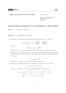
Example 5.4 Consider the system on R2 ,
1
x˙ 1 = − x2 + u
2
1
x˙ 2 = x1
2
Note that f (x1 , x2 ) = 21 (−x2 , x1 ) and g(x1 , x2 ) = (1, 0). The drift vector field f is weakly positively Poisson
stable (as its trajectories are closed, see Figure 1). On the other hand,
1
[f, g] = (0, − )
2
and hence dim C(x) = n for all x ∈ R2 . Therefore, the system is globally controllable. The result has an
intuitive explanation. One uses the input to get to the orbit of f that contains the desired goal point, and
once there, then waits until the system reaches the desired goal point.
•
9
MAE281b – Nonlinear Control
c 2008-2015 by Jorge Cort´
Copyright es. Permission is granted to copy, distribute and modify this file, provided that the
original source is acknowledged.
5 NONLINEAR TESTS FOR CONTROLLABILITY
x ’ = − 1/2 y
y ’ = 1/2 x
4
3
2
y
1
0
−1
−2
−3
−4
−4
−3
−2
−1
0
x
1
2
3
4
Figure 1: Trajectories of the weakly positively Poisson stable drift vector field of Example 5.4.
What if we cannot counteract the drift with our input vector fields? Let us present a more general set of
sufficient conditions for systems that do not fall under the hypotheses of Proposition 5.1. Here, we follow [5].
We say that a Lie bracket in {f, g1 , . . . , gm } is bad , if it contains an odd number of f factors and an even
number of each gk factors. Otherwise we say it is good . The degree of a bracket is the total number of vector
fields of which it is comprised. For instance the bracket [f, [[f, g1 ], [f, g2 ]]] is good of degree 5, and [[f, g1 ], g1 ]
is bad of degree 3. Let Σm denote the permutation group on m symbols. For σ ∈ Σm and B a Lie bracket
of {f, g1 , . . . , gm }, define σ
¯ (B) to be the bracket obtained by fixing f and changing gk by gσ(k) , 1 ≤ k ≤ m.
Now define
X
σ
¯ (B) .
β(B) =
σ∈Σm
A sufficient conditions for small-time local controllability is the following.
Theorem 5.5 (Sussmann [5]) The system (1) is small-time locally controllable from x0 if dim C(x0 ) = n
and every bad bracket B has the property that β(B)(x0 ) is a linear combination of good brackets, evaluated
at x0 , of degree lower than B.
Example 5.6 ([5]) Consider the single input system
x˙ = u
y˙ = x
z˙ = x3 y
Note that f = (0, x, x3 y) and g = (1, 0, 0). Let us compute the accessibility distribution. Consider the Lie
10
MAE281b – Nonlinear Control
c 2008-2015 by Jorge Cort´
Copyright es. Permission is granted to copy, distribute and modify this file, provided that the
original source is acknowledged.
6 OBSERVABILITY
brackets
[g, f ] = (0, 1, 3x2 y)
[f, [g, f ]] = (0, 0, 2x3 )
[g, [g, f ]] = (0, 0, 6xy)
[f, [f, [g, f ]]] = 0
[f, [g, [g, f ]]] = [g, [f, [g, f ]]] = (0, 0, 6x2 )
[g, [g, [g, f ]]] = (0, 0, 6y)
[g, [g, [f, [g, f ]]]] = (0, 0, 12x)
[g, [g, [g, [f, [g, f ]]]]] = (0, 0, 12)
Note that we have omitted brackets that are either zero or can be trivially expressed as a combination of
the brackets here. From the brackets above, we deduce that dim C(0) = 3, and hence the system is smalltime locally accessible from 0. What about controllability? Note that any bracket of degree ≤ 5 is a linear
combination at 0 of the good brackets g and [g, f ]. Any bracket of total degree 6 has to be good (why?).
And we certainly do not have to worry about brackets with degree higher than 6 (why?). Therefore, using
Theorem 5.5, we conclude that the system is locally controllable from 0.
•
6
Observability
Consider the MIMO system (2). Let us start by defining what we understand by observability. For convenience, let y(t, x0 , u) denote the output of the system starting with initial condition x0 under input function u.
Definition 6.1 Two states x1 , x2 ∈ Rn are said to be indistinguishable (denoted x1 Ix2 ) if, for every admissible open-loop input function u, the output function t 7→ y(t, x1 , u) of the system with initial state x(0) = x1 ,
and the output function t 7→ y(t, x2 , u) of the system with initial state x(0) = x2 are identical in their common
domain of definition. The system is observable if x1 Ix2 implies that x1 = x2 .
In other words, if the system is observable, we can distinguish between different states by means of the output
functions. Note that this definition of observability does not imply that every input function distinguishes
points of Rn . However, if the output is the sum of a function of the initial state and a function of the input
(as it is for linear systems), then it is easily seen that if an input distinguishes between two states, then every
input distinguishes them.
Our objective in this section is to come up with a nonlinear version of the Kalman rank condition for
observability of linear systems. It will be convenient for us to consider a “local” version of Definition 6.1.
Basically, x1 I V x2 , where V is an open set that contains both x1 and x2 , if for every admissible open-loop
input function u : [0, T ] → U with the property that the solutions starting at x1 and x2 both remain in V
for t ≤ T , the output functions t 7→ y(t, x1 , u) and t 7→ y(t, x2 , u) are identical for t ≤ T in their common
domain of definition.
Definition 6.2 The system (2) is locally observable at x0 if there exists a neighborhood W of x0 such that,
on any neighborhood V of x0 contained in W , the relationship x1 I V x2 implies x1 = x2 . If the system is
locally observable at each x0 , then the system is locally observable.
Roughly speaking, the system is locally observable if every state can be distinguished from its neighbors by
using system trajectories remaining close to the state.
11
MAE281b – Nonlinear Control
c 2008-2015 by Jorge Cort´
Copyright es. Permission is granted to copy, distribute and modify this file, provided that the
original source is acknowledged.
6 OBSERVABILITY
Example 6.3 Consider the system
x˙ = u
y1 = sin x
y2 = cos x
The system is locally observable. However, the system is not observable since points that differ by 2π are
indistinguishable.
•
Just as the accessibility distribution was critical for accessibility, we will see that the observation space plays a
key role for observability. The observation space O is the linear space of functions on Rn containing h1 , . . . , hp
and all repeated Lie derivatives
LX 1 LX 2 . . . LX k h j ,
j ∈ {1, . . . , p}, k = 1, 2, . . .
where Xi ∈ {f, g1 , . . . , gm }. An interesting interpretation of the observation space is as follows: from its
definition, we can see that O contains all the output functions as well as all the derivatives of the output
functions along the system trajectories.
We are interested in determining how many independent functions are in the observation space. With this
goal, define the observability codistribution as
dO(x) = span{∇H(x) | H ∈ O}.
The following result gives a computable test for local observability.
Theorem 6.4 Consider (2) and let x0 ∈ Rn . Then the following holds:
(i) If dim dO(x0 ) = n, then the system is locally observable at x0 ;
(ii) If dim dO(x) = n for each x, then the system is locally observable.
Example 6.5 Consider Example 6.3. Note that O = {a sin x + b cos x | a, b ∈ R}. Therefore, dim dO(x) = 1
for all x ∈ R, and the system is locally observable.
•
The following result is similar to the ones for accessibility. It states that the sufficient condition for local
observability is “almost” necessary.
Proposition 6.6 If the system (2) is locally observable, then dim dO(x) = n on an open and dense subset
of Rn .
The result in Proposition 6.6 is sharp, as the following example shows.
Example 6.7 Consider the system
x˙ = 0
y = x3
This system is clearly observable. However, O = {ax3 | a ∈ R}, and therefore, dO(0) = 0.
•
The sufficient condition for observability is indeed necessary if the system is analytic and locally accessible.
Proposition 6.8 Assume (2) is locally accessible and analytic. Then dO is constant-dimensional. In particular, the system is locally observable if and only if dim dO(x) = n for each x.
12
MAE281b – Nonlinear Control
c 2008-2015 by Jorge Cort´
Copyright es. Permission is granted to copy, distribute and modify this file, provided that the
original source is acknowledged.
REFERENCES
REFERENCES
References
[1] H. Nijmeijer and A. J. van der Schaft, Nonlinear Dynamical Control Systems.
Springer, 1990.
[2] E. D. Sontag, Mathematical Control Theory: Deterministic Finite Dimensional Systems, 2nd ed., ser. TAM.
Springer, 1998, vol. 6.
[3] A. Isidori, Nonlinear Control Systems, 3rd ed., ser. Communications and Control Engineering Series.
1995.
Springer,
[4] H. J. Sussmann and V. Jurdjevic, “Controllability of nonlinear systems,” Journal of Differential Equations, vol. 12,
pp. 95–116, 1972.
[5] H. J. Sussmann, “A general theorem on local controllability,” SIAM Journal on Control and Optimization, vol. 25,
no. 1, pp. 158–194, 1987.
13
MAE281b – Nonlinear Control
c 2008-2015 by Jorge Cort´
Copyright es. Permission is granted to copy, distribute and modify this file, provided that the
original source is acknowledged.