
Information provision and consumer behavior: A
Information provision and consumer behavior: A natural experiment in billing frequency∗ Casey J. Wichman† University of Maryland, College Park April 7, 2015 Abstract In this study, I examine a causal effect of billing frequency on consumer behavior. I exploit a natural experiment in which residential water customers transitioned exogenously from bi-monthly to monthly billing. I find that customers increase consumption by approximately five percent in response to more frequent information. This result is reconciled in a model of price uncertainty, where increases in billing frequency reduce the distortion in consumers’ perception of price. Using treatment effects as sufficient statistics, I calculate gains in consumer surplus equivalent to 0.5–1 percent of annual water expenditures. Heterogeneous treatment effects suggest increases in outdoor water use. JEL Codes: D12, D61, H42, L95, Q21, Q25 Keywords: information provision, billing frequency, price perception, natural experiment, water demand, water conservation, welfare ∗ Author email: [email protected]. Author address: 2200 Symons Hall, University of Maryland, College Park, MD 20742. † I am grateful for discussions with Rob Williams, Lint Barrage, Maureen Cropper, Richard Just, Chris Timmins, Kerry Smith, Laura Taylor, Roger von Haefen, Anna Alberini, J.R. DeShazo, Dietrich Earnhart, Jacob LaRiviere, Jonathan Eyer, Evan Rogers, Steve Sexton, Lesley Turner, and Ginger Jin that greatly improved this manuscript. I am indebted to Martha Ziegler and other staff at the City of Durham water utility for providing the data used in this analysis. Additionally, I thank seminar and conference participants at the 2014 Southern Economics Association, the 2014 AAEA Annual Meetings, the 11th Annual International Water Resource Economics Consortium meetings, the CU Boulder Environmental and Resource Economics Workshop, the Heartland Environmental and Resource Economics Workshop, Duke University, North Carolina State University, University of South Carolina, American University, Resources for the Future, University of Massachusetts Amherst, Cornell University, University of Kansas, UCLA, and the University of Georgia for their insightful comments and suggestions. 1 1 Introduction Conventional economic wisdom implies that more information is typically better. For many consumer goods and services, however, the decision to consume an economic good is disconnected from its purchase price. In these contexts, providing consumers with more information may affect their behavior. For consumption of water or electricity, for example, information on consumption costs is limited because billing is infrequent. If this source of limited information distorts the price signal that consumers use to make decisions, then improving the clarity of this signal has implications for consumer welfare. Whether and how imperfect perception of prices and quantities affects consumer behavior is an empirical question of growing interest. A recent vein of literature suggests that consumers tend to underestimate prices, taxes, and quantities consumed that are transmitted opaquely or allow for customer inattention (Chetty et al., 2009; Grubb and Osborne, 2015). Empirical examples range from behavioral responses to tax-inclusive prices to improving the salience of consumption information through “bill shock” reminders for cell-phone use. A parallel literature on consumer behavior in environmental policy considers the impact of social norms (Ferraro and Price, 2013) and information provision (Jessoe and Rapson, 2014) and shows that informative interventions can reduce consumption and thus serve as an instrument of conservation. With few exceptions, previous research suggests that various information treatments can be utilized to reduce consumption of economic goods that impose external costs on society. Particularly in highly regulated markets for electricity and water demand where prices are politically difficult to change, finding cost-effective conservation strategies is of topical policy interest. However, no one has examined the effect of changes in the frequency of information on consumer behavior in intermittent choice settings. Further, the majority of the existing research on informative interventions as a tool for conservation stops short of estimating changes in welfare, with Allcott and Taubinsky (2015) being a notable exception for the 2 purchase of energy efficient lightbulbs. In this paper, I make several contributions to this growing literature with an application to the management of a pertinent environmental resource. I take advantage of a natural experiment in which residential water customers are exposed to exogenous increases in billing frequency within a single water provider’s service area in the southeastern United States. I find strong empirical evidence that the provision of more frequent information increases water consumption by approximately five percent. This result contrasts the findings of previous work and has significant implications for efficient management of scarce environmental resources. Similar to repeated interventions, I find a lasting effect within the 4.5-year study period. I show that households transition quickly to a new baseline equilibrium in which long-run treatment effects are consistently larger than the magnitude of the short-run effect. My empirical results necessitate a closer examination of the mechanism driving consumer behavior in response to more frequent information. To that effect, I motivate a conceptual model of imperfect price perception that reconciles my empirical findings with the current literature on salience and inattention. Based on the notion that consumers are receiving more frequent information about the price of water with the receipt of monthly (versus bimonthly) bills, the information “treatment” allows consumers to update their perception of price.1 This framework is general enough to accommodate the findings of previous research since more frequent information nudges consumers closer to the neoclassical ideal of decisionmaking under perfect information. As a motivating example, a consumer who initially underperceives the price of electricity can be modeled similarly to a customer who over-perceives the price of water, since more frequent billing will reduce the wedge between her perceived price and the actual price. Further, I develop a transparent welfare framework using treatment effects as sufficient statistics for consumer demand. Since a consumer who misperceives price and thus consumes suboptimally from her perfectly informed self will be better off upon the receipt of new infor1 Bi-monthly bills refer to customer bills that are received every two months. 3 mation, there are welfare gains from the provision of more frequent information. Consumer surplus measures suggest a welfare gain of approximately 0.5 to 1 percent of annual household expenditures on water that are attributable to the change in billing frequency. The empirical setting is an exogenous transition of residential water customers from bimonthly to monthly billing within a single water utility. Beginning in 2011, the City of Durham’s Department of Water Management in North Carolina transitioned residential customers in geographically differentiated billing districts to monthly billing over the course of two-and-a-half years. By exploiting the assignment of monthly billing, I estimate an average treatment effect on water consumption due to increased billing frequency at the household level. The primary result is that households billed monthly consume approximately five percent more water than households billed bi-monthly. I show that this effect is robust to unobserved neighborhood effects by examining household consumption before and after the change in frequency within 500 feet of common billing group boundaries. Treatment effects are found to persist over time with a long-run treatment effect implying an approximately ten percent increase in water use. Further, I estimate conditional average treatment effects that indicate an increase in outdoor water use in the summer months. I also find important heterogeneity among baseline water use, lot size, and assessed home value. From an environmental policy perspective, informative signals are being used increasingly as a regulatory instrument in the context of electricity and water conservation. The findings of this paper suggest that increases in billing frequency can have the perverse effect of increasing consumption. This result is particularly poignant because the efficient price for residential water is its long-run marginal cost of provision (Timmins, 2002; Olmstead and Stavins, 2009). However, since the market price is likely set below its efficient level (Mansur and Olmstead, 2012), the demand response to more frequent information may exacerbate the wedge between privately and socially optimal consumption levels. In the next section, I motivate a conceptual framework to explore changes in billing frequency. In Section 3, I describe the data used in the analysis and outline the empirical 4 setting. I present a series of quasi-experimental models to estimate a causal effect of information provision on consumer demand as well as heterogeneous treatment effects in Section 4. In Section 5, I discuss the results and implications of the empirical models, while I estimate associated welfare changes in Section 6. The final section concludes. 2 Background and conceptual framework Consider the choice setting in which a consumer is deciding how much water to use in a given billing period.2 Borenstein (2009), Gilbert and Graff Zivin (2014), Harding and Hsiaw (2014), and Wichman (2014), for example, motivate models of behavior based on prices, quantities consumed, and behavior in previous periods as heuristics for making consumptive decisions in electricity and water demand. Since utility bills are received periodically, the arrival of billing information offers consumers an opportunity to update their consumption in response to external feedback regarding their behavior. A change in the frequency of billing information is particularly relevant in the intermittent choice setting for water use since consumers generally do not know how much water they are using at any point in time, nor how much water an appliance uses and its associated variable costs. Thus, more frequent billing allows a consumer to better align price signals directly with the usage of appliances or water-intensive behavior. With a fuzzy link between water consumption and the receipt of a water bill, however, the consumer may not have perfect information about prices and consumption that neoclassical models of consumer demand require. Several papers have documented this behavior theoretically and empirically in different markets. Numerous studies show that: 1) obtaining the relevant information to make perfectly informed decisions is costly (Shin, 1985; Sallee, 2014; Caplin and Dean, 2014); 2) consumers may be inattentive to or unaware of (changes 2 While the model presented in this paper is generalizable to many choice settings in which consumption of the economic good and payment for consumption are separated temporally (e.g., cell phone usage, credit card purchases, electricity demand, and so forth), the discussion henceforth will consider water consumption to motivate the empirical setting. 5 in) prices or taxes (Sexton, 2014; Chetty et al., 2009; Finkelstein, 2009; Li et al., 2014; Houde, 2014); 3) inattention could be a function of attributes that are “shrouded” from consumers (Gabaix and Laibson, 2006); 4) consumers may use heuristics for decision-making when price and quantity information is opaque or uncertain (Borenstein, 2009; Ito, 2014; Wichman, 2014); or 5) consumers may have biased perceptions of prices, expenditures, and consumption (Allcott, 2013; Grubb and Osborne, 2015; Bollinger et al., 2011).3 Thus, relaxing the notion that consumers respond with perfect information for water use should not be met with much criticism. But, the question remains: how are consumers using price and quantity information to make decisions in intermittent choice settings? Many researchers examine this question in framed field experiments in the context of water and electricity demand to examine quantity reminders, social norms, and other forms of informative interventions (Allcott, 2011; Ferraro and Price, 2013; Kahn and Wolak, 2013; Jessoe and Rapson, 2014; Brent et al., 2014). But, no studies have focused on an information treatment as simple as the provision of more frequent billing information, which is arguably the easiest form of information provision to implement as policy. In the conceptual model presented below, the general static setting is one in which a consumer is planning for water consumption and expenditures conditional on her preferences, technology stock, past usage, and prevailing market prices. Then, the consumer is provided with an information shock— the receipt of a utility bill. The bill allows consumers to learn about their past usage and prices paid for water and update their consumption habits accordingly.4 In this framework, the customer’s bill serves as a familiar mechanism for receiving information, but provides new price and quantity information to the consumer when it arrives. This treatment mechanism stands in contrast to many recent field experiments in which consumers are given a foreign source of information about their consumption.5 The drawback of 3 This literature complements research that examines the effect of informative signals of product quality on consumer behavior (c.f., Foster and Just (1989) or Jin and Leslie (2003)). 4 An example of a utility bill, which serves as the information “treatment” in this paper, is included as Figure A.1 in the appendix. 5 For example, social comparisons among use and expenditures (Ferraro and Price, 2013; Allcott, 2011; Costa and Kahn, 2013; Brent et al., 2014), educational materials about complicated rate structures (Kahn 6 the natural experiment in this paper is the inability to control the mechanism through which consumers may respond, though this is not guaranteed in field or lab experiments (Ludwig et al., 2011), as well as the lack of pure randomization. The primary benefit, however, is that consumers are familiar with their typical utility bill, so it is perhaps more likely that they will simply adjust their behavior along an existing margin. That is, consumers will update whatever decision rule they use to make water consumption decisions, rather than constructing a new rule in response to a foreign information intervention. In this context, consumers are not receiving more nor better information about their consumption, they are simply receiving the same information more frequently. To the extent that this is true, the natural experiment isolates a consumer response along the frequency of information provided, rather than the quality or quantity of information provided. Thus, any prevailing misperceptions within a consumer’s decision-making process are plausibly mitigated with more frequent information of the same type. In the limit, increasing the frequency of information provided to consumers (i.e., realtime feedback) should tend toward the neoclassical ideal of perfect information.This notion corresponds to a “pure nudge,” in the parlance of Allcott and Taubinsky (2015), that corrects the informational failure completely. With less frequent information (e.g., periodic utility bills), however, consumers are more likely to base their consumptive decisions on imperfect information. So, if a consumer receives a more frequent signal about her consumption, she may change her behavior in such a way that aligns more closely, but not perfectly, with standard models of consumer demand. This example provides the groundwork for the conceptual setting in which water customers alter consumption in response to an increase in the frequency of bills to capture information rents. Allowing for ex post misoptimizing behavior in this choice setting deviates from the behavioral welfare frameworks of Chetty et al. (2009) and Allcott and Taubinsky (2015) at the cost of specifying a positive model of consumer behavior. and Wolak, 2013), real-time feedback on consumption (Jessoe and Rapson, 2014; Gans et al., 2013; Strong and Goemans, 2014), or informative signals on variable costs of durable goods (Allcott and Taubinsky, 2015). 7 2.1 Billing frequency and price misperception In this subsection, I develop a model of misperceived price such that a consumer who receives more frequent information about her consumption habits may choose to consume more or less water since she has a more accurate perception of water prices for her consumption in each billing period. Finkelstein (2009), Li et al. (2014), and Sexton (2014) find that consumers tend to misperceive (changes in) prices or taxes that are not salient. Thus, increasing billing frequency is a plausible mechanism to increase the salience of water prices. Consider a consumer with utility over water consumption (w) and a composite good (x): u = x + aw1/γ+1 (1) where utility is quasilinear in x and preferences over w exhibit constant elasticity of demand. The consumer observes the budget constraint, M = x + p˜w, where her wealth (M ) equals expenditures on x with its price normalized to unity and her perceived expenditures on water. The budget constraint is satisfied with equality since any residual consumption is allocated to the composite good. The price a consumer perceives for her consumption of w is defined as p˜ = θp where p is the true price and θ is a perception parameter that specifies the degree to which she over or underestimates the true price. A consumer with perfect information is represented by θ = 1. While previous research bounds this parameter from above at unity, I allow for misperceptions to deviate above and below the true price since there is no good theoretical foundation for why an inattentive consumer would always under-perceive prices. The water provider can manipulate θ by changing information available on an intermittent bill, changing the frequency at which consumers are billed, allowing customers to automatically deduct their bill from their checking account, and so forth. To coincide with the empirical analysis, define θ as a function of billing frequency, BF, and a vector of other fixed characteristics, Z, θ = f P (BF, Z). 8 (2) Equation 2 captures the essence of the analysis that follows—changes in billing frequency affect demand by altering consumers’ perception of price. As a useful, and plausible, assumption, I restrict information to be weakly welfare improving: Assumption 1 More frequent billing information can never make anyone worse off. That information is welfare improving simply means that consumers can always choose to be ignorant, and that there are no cognitive costs to ignoring new information. There may, in fact, be cognitive costs to processing this information, but the consumer will only undertake such an action if its benefits exceed costs at the margin. This assumption implies structure for the functional relationship in Equation 2. For θ > 1, increases in BF exhibit a negative effect on θ such that increasing billing frequency reduces the distortion between the true price and perceived price. However, I do not restrict θ to be greater than one. For θ < 1, the predicted response to BF is reversed, allowing for increases in information to decrease the wedge between the true price regardless of the direction of price misperception. Assuming f P is differentiable, we can write these effects on demand via the envelope theorem, 2 >0 ∂w(˜ p) ∂ w(˜ p) = =0 ∂θ∂BF ∂BF < 0 if θ > 1 if θ = 1 . (3) if θ < 1 Since θ is unknown to the researcher, it is unclear a priori whether a consumer perceives a price that is higher or lower than the true price p. Hence, the demand response to an increase in the frequency of billing information is ambiguous and depends on the initial degree of price misperception. Further, Equation 3 implies that the direction of the demand response (∂w/∂BF) reveals consumers’ initial misperceptions of price. As an illustrative example, consider a consumer facing a change in the perceived price of water induced by an increase in billing frequency. In Figure 1, let DE be the consumer’s 9 initial misperceived budget line under the bi-monthly billing regime with a corresponding perceived price, p˜0 . Due to misperceptions of the price of water, she targets the consumption bundle (x, w) ¯ at the beginning of the billing cycle, but consumes the bundle (¯ x, w) ¯ since she over-perceives the price of water (θ > 1) and, hence, allocates more consumption to the numeraire good. Upon updating her perception of price through more frequent billing, she learns that her true budget line is DF and chooses (x? , w? ) as the preferred allocation.6 This movement corresponds to an increase in water consumption in response to a reduction in the wedge between her initial misperception and her updated perception of price. Additionally, the preferred bundle indicates an increase in consumer welfare. 2.2 Welfare effects from price misperception Since the misperception of prices from infrequent billing drives a wedge between the actions of a perfectly informed consumer and an inattentive consumer, there are welfare gains from information provision. If θ were observable to the researcher, the change in welfare could be obtained by measuring the area under the demand curve between the implied changes in perceived price. However, since θ is an unknown parameter, I rely on behavioral welfare analyses similar to that of Allcott and Taubinsky (2015), Chetty et al. (2009), and Just (2011) to obtain sufficient statistics from observable or estimable parameters that allow for welfare analysis when consumers may not optimize perfectly.7 In particular, consider an increase in the frequency of information, represented by θ0 to θ1 , that corresponds to a change in perceived price from p˜0 to p˜1 . Assumption 1 allows us to remain agnostic about the initial misperception of price since a positive demand response to an increase in information implies that consumers display positive θ, and the converse is also true. Under the notion that perceived price tends towards the true price with an increase in 6 Note, however, that misperceptions need not be fully corrected in this framework. The welfare analysis differs from other work in behavioral welfare analysis in that I specify a positive model of demand that may be driving behavior in this setting whereas Chetty et al. (2009), for example, use price and tax elasticities to identify preferences when consumers make optimization mistakes. 7 10 billing frequency, I make the following assumption as a useful benchmark: Assumption 2 Under the more frequent billing regime, ex post perceived prices are proportional to the true price. While strong, this assumption allows the researcher to back out perceived prices from observable changes in demand. Assumption 2 is reflective of the pure nudge assertion in Allcott and Taubinsky (2015) and Chetty et al. (2009), in which the informational treatment is fully corrective; ex post proportionality to the true price weakens this assumption. With respect to real-time feedback through smart-metering technology, it is possible that consumers do in fact know the marginal price they are paying at any point within the billing cycle. Strong and Goemans (2014) and Kahn and Wolak (2013), for example, show that consumers tend to optimize “better” under block rate structures when provided with real-time consumption feedback and educational treatments on how their bill is calculated, respectively. In any case, monthly billing provides an opportunity for price misperception to prevail after the change in billing frequency. To derive an empirically tractable measure of θ, we can write the constant elasticity of demand with respect to perceived price, ηP = %∆w(˜ p) , %∆˜ p (4) which holds by definition. The percent change in perceived price can be used to obtain an empirical measure of the change in the perception parameter by observing a change in quantity demanded. In particular, we can write, %∆˜ p= p˜0 θ0 p −1= − 1 = %∆θ, p˜1 θ1 p (5) since the market price does not change. Combining this expression with Equation 4, rear- 11 ranging, and multiplying through by p˜1 provides, ∆˜ p = ∆θp˜1 = %∆w(˜ p) ηP p˜1 , (6) where p˜1 is the ex post perceived price that is proportional to p, that is p˜1 = αp with α being the degree of ex post misperception via Assumption 2. Equation 6 states that a change in perceived price is simply a function of the market price, the perceived price elasticity, and the corresponding demand response. This expression is convenient since η P can be estimated or inferred from other studies and the change in water consumption can be estimated using quasi-experimental techniques. Since Equation 6 describes the change in perceptions of price due to a change in an unobserved parameter, I utilize Assumption 2 to provide a reference point (i.e., the observable price) to obtain a price-equivalent, in dollars per unit of water consumption, of the consumer’s perceived price. Using this measure of the consumer’s ex post perceived price, consumer surplus can be calculated by integrating the demand function between the initial price perceived, p˜0 , and the price perceived after the change in billing frequency, p˜1 , Z p˜0 ∆CS = p˜1 ∂w 1 , w(˜ p)d˜ p∼ = − ∆θp˜1 2 ∂BF (7) which is analogous to the Harberger (1964) triangle approximation for deadweight loss since the data in the experiment are not sufficient to estimate a true demand function.8 Under the assumptions made so far, the treatment effect (∂w/∂BF) and the perceived price elasticity of demand (η P ) serve as sufficient statistics for calculating changes in welfare due to a change in billing frequency. 8 Note that welfare calculations are simplified by assuming quasilinear preferences. As such, equivalent and compensating variation are identical and estimate consumer surplus exactly (Hausman, 1981). 12 3 Empirical setting Beginning in December 2011, the City of Durham’s Department of Water Management in North Carolina (henceforth, “Durham”) transitioned individual billing districts from bimonthly to monthly billing at different points in time. Primary reasons for the transition include cost-saving from fewer delinquent payments, early leak detection, improving customer service, and reducing administrative costs. In addition, the change in billing frequency was enabled by district-wide installation of automated meter reading devices. The new meters allow for consumption levels to be obtained via radio frequency such that the costs to read meters manually were reduced. Meters were installed for each billing district and, once the installations were completed, the entire district was transitioned to monthly billing. Customers were notified of the transition to monthly billing by mail approximately six weeks before the transition.9 To make a cost-saving argument to the city council, the water utility used a single billing district as a pilot group to measure changes in administrative costs before and after the transition to monthly billing cycles. After that, billing districts were transitioned to monthly billing according to meter installation and administrative schedules. The order of districts for meter installation (and, subsequently, monthly billing) was chosen to work around billing cycles and other feasibility constraints. According to utility officials, no consideration of billing history, income base of neighborhood, or any other financial indicator was taken into account when choosing which districts to transition.10 Given these details, the assignment of monthly billing is plausibly exogenous to the 9 A copy of the mailer distributed to customers is included as Figure A.2 in the appendix. In Table A.1, I present regression results that predict the likelihood of a billing district to be transitioned from bi-monthly to monthly billing based on observable household characteristics. In particular, I consider the first district to transition in a probit model, as well as the sequential transition of routes in an ordered probit framework. The former suggests that lot size, household size, and the number of bedrooms increased the probability of the pilot group being chose, while the square footage of the home and number of bathrooms decreased the probability. There is weak evidence that smaller water bills are correlated with initial treatment. Further, the ordered probit reveals that the age of a home is weakly negatively correlated with the order of transition, while all other observable factors are insignificant. These results suggest that treatment selection on observable household characteristics is not a significant concern. 10 13 household, conditional on residing within a particular billing district. The household has no ability to manipulate the assignment of billing frequency short of moving across billing cycle boundaries. Within the study period, 12 of 17 billing districts were transitioned according to the timing in Table 1. The first district transitioned received their first monthly bill on December 1st, 2011. Figure 2 presents a map of the first six billing districts to transition to monthly billing (in Panel A) and all districts transitioned to monthly billing by June 2014 (in Panel B). The entire service area is represented by the union of all billing districts outlined in bold. In Panel C of Figure 2, I present a maginified view of billing district boundaries within neighborhoods. This figure illustrates that the district boundaries are designated in such a manner that neighbors could be consuming water concurrently, but may be billed at different frequencies. Thus, this design allows for the exploitation of geography to minimize the concern that differences in neighborhood characteristics might bias results. 3.1 Data The primary data used in this analysis are residential billing records for Durham water customers. Included in these data are (bi-)monthly water and sewer use, fixed service fees and volumetric consumption rates, the address of the customer, billing district, and whether a customer has their water bill automatically deducted from a bank account. The billing data were matched by address with geocoded tax assessor data, containing structural characteristics of the home, obtained from Durham County. Each matched residential address was spatially linked to its 2010 Census block as well as billing district polygons provided by Durham. For each household, I determine the nearest billing district, as well as the linear distance from the centroid of the tax parcel its nearest district boundary. Key demographic variables from the 2010 SF1 Census are matched to each household’s Census block. Residential premises that changed water billing accounts within the timeframe of the study are removed from the sample—this strategy reduces the impact of renters, who may not pay water bills explicitly. Further, this avoids econometric identification problems when relying 14 on variation within a household over time.11 The final sample consists of roughly 59,000 individual household accounts with water bills from February 2009 through June 2014, which implies slightly less than 1.7 million householdby-bi-monthly unique observations. Summary statistics for variables of interest are presented in Table 1. The first four columns decompose household characteristics and details on water use by the year in which households transitioned from bi-monthly to monthly billing. Summary statistics in the final column are for the entire sample. Each of the treatment waves are relatively similar across demographic, water use, and housing characteristics, and similar to the sample mean, with the exception of households that transitioned in 2013 along several dimensions. For this group, home value (a proxy for wealth) is notably larger than that of all other groups. Further, these households tend to have larger homes on larger lots, and are more likely to be located in a Census block with fewer renters and a higher proportion of white residents. Water consumption, however, is statistically similar across all groups. For the typical household in the sample, the mean assessed home value is approximately $186,000 with a standard deviation of $126,000. The average home is on one-third of an acre, 34 years old, roughly 1,800 square feet, with three bedrooms. Within the final sample, households reside in Census blocks in which approximately one-quarter of all homes are renter-occupied. 53% of the sample is white and the average household size is between two and three people. Average bi-monthly water bills for all time periods in the sample are $85 for consumption of 985 cubic feet of water. Further, I include weather covariates obtained from the North Carolina State Climate Office. The key variables used are mean maximum temperature for a 60-day rolling window that is backwards-looking from the date each individual bill was mailed. The sum of rainfall (in inches) for the same 60-day time window is also calculated. A final caveat is that under bi-monthly billing, water bills are mailed on a staggered 11 Renters may cause problems for identification if they do not receive a water utility bill. However, this effect would tend to pull any estimated treatment effect towards zero so long as renters did not change their behavior at exact time of the change in billing frequency. 15 schedule that smooths administrative work and meter reading throughout the year. As an example, a billing district on the odd cycle may receive a bi-monthly bill in March for consumption in January and February. Contrarily, a billing district on the even cycle would receive a bill in April for consumption in February and March. Rather than dealing with these two groups independently, I pool households into two-month cycles corresponding to the date in which bills are received, but allow for each district to retain accurate measures of weather fluctuations within their use period. As such, there are 32 distinct time periods in the study that correspond to two-month windows between February 2009 and June 2014. Additionally, since monthly bills account for consumption during a shorter duration than bi-monthly bills by construction, monthly consumption is aggregated to a bi-monthly level. So, the unit of observation for consumption is a two-month period regardless of whether households are being billed monthly or bi-monthly. 3.2 Prices The transition of households to monthly billing provides a unique natural experiment to identify a causal effect of more frequent information on consumer behavior so long as other factors are not changing at the same time. When households were transitioned from bimonthly to monthly billing, fixed water and sewer service fees were cut in half as well as block cut-offs in the tiered rate structure. Marginal volumetric rates for consumption remained constant across billing frequencies. Figure A.3 illustrates the change in the rate structure for monthly and bi-monthly billing. The solid line is the increasing block rate structure used to calculate bi-monthly bills, while the dotted line is used to calculate monthly bills for the 2012-2013 fiscal year. As shown, the marginal prices for consumption do not change between monthly and bi-monthly rate structures, but the quantity blocks for consumption are halved for each price tier. This structure was adopted to ensure that customers transitioned to monthly billing were charged at the same rate as bi-monthly customers. Thus, for the same level of consumption, 16 two monthly bills are equivalent to one bi-monthly bill in dollar amounts. While this is a mechanical interpretation of the notion that prices did not change, the change in the block endpoints could affect consumer behavior. It is not clear, however, in what direction this change might bias results, but the extent to which this bias exists depends on whether consumers know and use the tiered rate information to make decisions. Since the water utility bill includes no information about the block rate structure (see Figure A.1), it is unlikely that consumers are responding to changes in the rate structure itself.12 Further, Wichman (2014) shows that water customers, and Ito (2014) for electricity customers, exhibit behavior that corresponds to changes in average price, or the total bill, when facing increasing block rates, which eases this concern. 3.3 Technical efficiency of new meters The primary threat to the unconfoundedness assumption in the empirical strategy is that billing districts were transitioned to monthly billing directly after new meters were installed. It is generally accepted in the water utility industry that as meters age, they fail to register all water that passes through. The typical advertised increase in technical efficiency is around the magnitude of 1-2%. Indeed, metering companies market the efficiency of new meters as a means to capture “non-revenue” water that utilities are treating and distributing, but is not showing up as billed consumption. Given this, it is possible that a switch to new meters may increase water “consumption” mechanically through the adoption of a more technically efficient metering system. Through a suite of empirical tests and robustness checks, I find no evidence that the empirical results are driven by technical efficiency improvements. 12 As further evidence, I present the empirical density of consumption in Figure A.4 in the appendix. In this figure, there is no evidence of bunching at the block rate cut-offs for consumption in the calendar year prior to treatment. 17 4 Empirical strategy The empirical approach I take in this paper identifies demand responses to an increase in billing frequency using quasi-experimental techniques. I regard the transition from bimonthly to monthly billing as the treatment, whereas households that, at any point in time, are billed on a bi-monthly basis serve as controls. To estimate the average treatment effect (ATE) of a change in billing frequency empirically, the following log-linear equation is specified, ln (wijt ) = α + βBFjt + Ct ω + Zijt γ + τt + ijt , (8) where wijt is household i’s water consumption in time t in billing district j.13 BFjt is a dummy variable equal to one if the billing district j is billed monthly at time t and zero otherwise. Ct is a vector of weather variables including mean maximum temperature (degrees Fahrenheit) and total rainfall (inches) for each billing period. Zijt is a vector of household and demographic characteristics described in Table 1. τt is a vector of time controls including some combination of time fixed effects, a linear time trend, and seasonal indicators. ijt is the residual error term. Treatment status is assigned to households if they reside in a billing district that is billed monthly at time t. In this specification, β will capture a causal effect of the change in billing frequency on water consumption, conditional on common trends between treatment and control, as well as standard exogeneity assumptions. Since the assignment of treatment is plausibly exogenous, it is worth noting the lack of potential selection bias. Selection into (or out of) treatment is not likely to occur since it would require households to move premises with the intention of sorting along billing district boundaries, which are not publicly ob13 In all regression specifications with logged dependent variables of water consumption, I add 1 to bimonthly water use since there are a small number of true zero use observations in the data set. All models were also estimated with consumption levels as the dependent variable and the results are unaffected. These estimates are available upon request. 18 servable. Additionally, all households are treated with monthly billing eventually, so even if there was an incentive to move premises to seek (or avoid) monthly billing, a sophisticated consumer would know that the benefit is unlikely to remain for long. Under these assumptions and common trends in pre-treatment water use between treatment and control, β is an unbiased estimate of the ATE and is equivalent to the average treatment effect on the treated (in the absence of selection). To analyze common trends, I first note that treatment and control households reside in a small geographic area, and sometimes within the same neighborhood (see Figure 2, for example). So, there is no reason, a priori, to think that consumption would exhibit different trends, or even different levels, since all households are exposed to common weather, annual rate increases, and other exogenous utility-specific shocks. Further, most control households eventually become treatment households within the study, so households that are treated later in the study serve as controls for households treated earlier in the study. Regardless, I explore mean consumption levels graphically for all households that eventually transitioned to monthly billing relative to households who never transitioned to monthly billing within the study. Figure 3 compares mean usage for both treatment and control groups in each time period. The control households (solid trend line) track the treated households (dashed trend line) closely before the first monthly bill represented by the vertical line in December 2011. There are slight deviations from this trend in the peak summer months prior to December 2011, but nothing extreme enough to invalidate common trends. While a simple linear regression approach presented in Equation 8 provides a consistent estimate of the ATE, it is possible that there are unobservable factors within households that influence water consumption. Preferences for the environment or water-intensive durable goods are likely candidates for variables that may affect a household’s response to the frequency of water bills, but the available data do not permit for direct controls. As such, I estimate Equation 8 with household-specific intercepts that absorb time-invariant 19 unobservable characteristics, ln (wijt ) = αi + βBFjt + Ct ω + τt + ijt (9) where αi is now a household-specific fixed effect. The identifying assumptions for β to remain a causal effect of billing frequency remains the same as before, though we now require strict exogeneity and conditional independence of the household-specific intercepts. The latter assumption indicates that treatment status cannot be correlated with an unobservable, timevarying factor at the household-level. Exogenous assignment of monthly billing across billing districts implies that treatment assignment did not target household characteristics explicitly. 4.1 Exploiting billing district boundaries To assess the robustness of the difference-in-difference estimates, I estimate treatment effects within a narrow window on either side of the billing district boundaries. I consider households within 2000, 1000, and 500 feet of district boundaries. I first estimate Equation 8 in a pooled cross-sectional framework since differencing out unobservables is unnecessary for identification of a local average treatment effect (LATE) in a regression discontinuity framework (Lee and Lemieux, 2010). However, I also estimate Equation 9 in this framework since there may be unobservables biasing results in the pooled cross-section. The latter specification, dubbed “difference-in-discontinuity,” takes account of the differences over time both within households and across treatment/control groups, while simultaneously limiting the set of included household observations based on distance from the nearest billing district boundaries (Grembi et al., 2012). The intuition behind the identification of a LATE in this scenario is that as one approaches the billing district boundary households become more similar, thus avoiding potential confounding factors in the difference-in-difference framework. Additionally, since there are control households on either side of a given district threshold at some point in time, the LATE identifies the relative difference of a treated household in the 20 same “neighborhood” as a control household over time. The main benefit of this approach is that it is robust to changes in unobservable neighborhood characteristics over time. To explore the appropriateness of these methods, I plot mean consumption for 2012 in 40 foot bins within 1000 feet of billing district boundaries. In Figure 4, treatment households, represented by solid diamonds on the right-hand side of each figure are the households in the first district to transition to monthly billing. Control households, represented by hollow circles on the left-hand side, are all other households. As shown, there is a clear deviation in the quadratic trend at the billing district boundary. While the control households display a more uniform, linear trend, treatment households have a larger variance and their consumption is generally increasing with the distance from the district boundary. The latter effect is likely driven by the initial treatment households residing in billing districts further from the city center and, thus, located on larger lots with higher demands for outdoor water (see Figure 2 for treated districts in the northern portion of the billing district, which is more rural than the central region). This differential use among treatment households is not problematic since the difference-in-discontinuity estimator is a consistent estimator of a LATE as the distance from the district threshold decreases in the limit and, as shown, the trends near the boundary threshold are relatively similar (Grembi et al., 2012). 4.2 Dynamic models of adjustment Since it is possible that any treatment effect observed is simply an initial response to more frequent information, but households revert back to initial levels of consumption, I specify dynamic models that include a lagged dependent variable as a covariate to control for inertia, that could include habit formation, in the consumption process. Similar to Gilbert and Graff Zivin (2014) the general estimating equation takes the form, ln (wijt ) = α + βBFjt + ζ ln (wijt−1 ) + Ct ω + Zijt γ + τt + ijt 21 (10) where, in an OLS framework, β remains the causal effect of interest in the short-run, which is augmented by an adjustment parameter, ζ. A long-run treatment effect is obtained from ˆ ˆ Additionally, the short-run ATE obtained the estimates of Equation 10, β ? = β/(1 − ζ). from estimation of Equation 10 provides a lower bound for the treatment effect based on the conditional independence assumption that states that past water usage is not correlated with treatment. The ATE estimated in Equation 9 and the ATE estimated in Equation 10 bound the treatment effect from above and below, respectively, which provides a useful robustness check of the true effect under different modeling assumptions (Angrist and Pischke, 2009). Further, since I rely on differencing out time-invariant unobservables for identification of a causal effect with correlated observations within a household, I estimate the panel analog of Equation 10. Consistent estimation of this model requires serial independence in the error terms for a given household, which is violated with certainty when using differencing methods to drop individual-specific intercepts (Nickell, 1981). However, I estimate this model for comparison with the OLS specification. 4.3 Heterogeneous responses to information provision I conclude the empirical analysis with an examination of heterogeneity in the estimated treatment effects. In particular, I focus on heterogeneity arising from subpopulations that may respond differentially to more frequent information. Formally, I estimate conditional average treatment effects (CATE) similar to Allcott (2011), Ferraro and Miranda (2013), and Abrevaya et al. (2014) by interacting covariates of interest with the treatment indicator. The CATE specification takes the form, ln (wijt ) = αi + βBFjt + X βs (BFjt × 1[Zijt ]s ) + Ct ω + τt + ijt (11) s∈S where βs captures the conditional average treatment effect for a series of S discretized variables in vector Zijt , and all else is the same as in Equation 9. Specifically, I consider indicators 22 for quintiles of each of the following covariates: pre-treatment mean (summer) consumption in 2009 and 2010, assessed home value as a proxy for wealth (Ferraro and Miranda, 2013), lot size as a proxy for irrigation intensity (Mansur and Olmstead, 2012; Renwick and Green, 2000), square footage of the home, age of the home, as well as the number of bathrooms within a household.14 Additionally, to expunge any source of endogeneity or mean reversion in the CATE estimation using (2009 and 2010) consumption patterns as conditioning covariates, I restrict the sample to observations beginning in January 2011 for models that explore heterogeneity based on pre-treatment water use. The conditioning variables chosen in Equation 11 either represent key drivers of residential water demand or serve as a proxy for preferences that may influence demand responses. As such, evidence of heterogeneous treatment effects along established margins allow for probing the mechanism through which consumers may be responding. In addition, I interact the treatment indicator with dummy variables for each season. Since informative interventions are largely used to induce conservation in environmental and resource policy, outdoor water use in the summer months is a key target for reductions in consumption. Finally, I explore the responsiveness of households who are enrolled in automatic bill payment (ABP) throughout the transition to monthly billing. These households provide two useful functions. First, under the notion that ABP customers are less attentive to changes in prices and, correspondingly, billing frequency (Sexton, 2014), a null treatment effect would instill confidence that the empirical results are identifying a behavioral response to the information treatment. Secondly, if these households do not display a response to the treatment, then it provides additional evidence that the ATE is not contaminated by an improvement in efficiency of the metering technology. 14 Note, I do not consider quantile treatment effects since I rely on household-specific intercepts to control for time-invariant unobservables. Within a fixed effect framework, quantile regression requires strong assumptions on rank preservation, which do not hold in this context. 23 5 Empirical results and discussion In this section, I present results motivated by the empirical models in previous section. First, Table 2 presents pooled OLS estimates of Equation 8. From Column (1) through (5), I add additional controls successively and analyze the coefficient on BF, the indicator for billing frequency. In each column, I present coefficients and robust standard errors clustered at the household level, as well as the billing district level, to account for serial correlation (Bertrand et al., 2004). The former accounts for the fact that water consumption is correlated within a household, whereas the latter acknowledges that the variation in treatment status arises at the billing district level. For all estimated ATEs, the sign is positive and each coefficient is significant at conventional levels. All other covariates have expected signs and significance. Collectively, the results imply that the transition to monthly billing increased consumer demand between five and nine percent, though the preferred specifications from this set of models are Columns (4) and (5), which control comprehensively for observable factors, exhibit the best fit, and also contribute the most conservative treatment effects. In Table 3, I present results that include fixed effects at the household-level to control for any time-invariant unobservables. The results suggest that any omitted variable bias from the OLS models in the previous table is likely small. The ATE of billing frequency is estimated at 8.4% and 4.6% increases in quantity of water demanded with the inclusion of seasonal and period-of-sample fixed effects, respectively.15 For comparison, the estimate of 4.6% in Column 2 of Table 3 can be compared directly with the estimate of 5.1% in Column 5 of Table 2, which could indicate a small positive bias from omitted factors. These estimates, however, are statistically similar. Moving forward, the estimate from Column (2) in Table 3 is the preferred estimate. This specification accounts for any time-invariant unobservables while simultaneously controlling for time effects. In terms of economic significance, this estimate is approximately half of the magnitude of water reductions called for during moderate to 15 For these estimates, a block bootstrap of t-statistics (with 200 draws) was performed both at the household and billing district level to account for serial correlation, as suggested by Bertrand et al. (2004). Inference on the coefficient of interest does not change. Results are available upon request. 24 severe droughts in North Carolina (Wichman et al., 2014). To examine whether there are unobservable changes in neighborhood characteristics that may bias the preferred ATE, I present regression discontinuity (RD) estimates (for the pooled cross-section) and difference-in-discontinuity (for fixed effects) estimates in Table 4. In Panel A of Table 4, pooled cross-section models are estimated for the set of households within 2000, 1000, and 500 feet of billing district boundaries. The treatment effect of billing frequency remains stable as the window shrinks, and remains significant at conventional levels.16 Further, I present results from the preferred fixed effects model, and similarly restrict the sample to the same households within 2000, 1000, and 500 feet of billing district boundaries in Panel B of Table 4. The estimates decrease monotonically moving from Column (1) to (3), while standard errors increase, but the results remain statistically similar under the more conservative standard errors. The estimate within 500 feet of billing district boundaries indicates a positive effect of billing frequency on water demand that is robust to unobservable timevarying factors at the neighborhood level. Standard errors clustered at the billing district level indicate that this effect is not statistically different from zero, but I note that this effect is statistically similar to that of Columns (1) and (2). Dynamic models presented in Table 5 imply that past water consumption is an important predictor of current water consumption and significantly improves the fit of each model. The treatment effect in the first two columns is smaller than that of the preferred specification (2.1% and 2.6%) but statistically different positive. Additionally, the estimate on the lagged dependent variable suggests that there is a relatively quick adjustment period (between one and two periods) to reach the new equilibrium. A long-run treatment effect is estimated at 10.5% and 6.6% in the OLS and fixed effects models, respectively. Since the fixed effects estimates are inconsistent (Nickell, 1981), the preferred estimate is from the OLS estimator, which suggests a long-run treatment effect that is double the magnitude of the preferred ATE in Table 3. As mentioned previously, the short-run effect in Column (1) provides a lower 16 The inclusion of a flexible polynomial for distance from the boundary cut-off (up to degree 3) has no effect on the treatment estimate nor the fit of the model. These results are available upon request. 25 bound on the true treatment effect, whereas the preferred estimate from the fixed effects models (4.6%) bounds the treatment effect from above (Angrist and Pischke, 2009). These results suggest that there is indeed a positive response to increases in information provision in water demand and that this effect appears to strengthen over time. Results from the dynamic models provide an interesting conclusion relative to previous research. While one-shot interventions of social norms and information provision tend to have an immediate effect that dissipates over time (Ferraro et al., 2011; Allcott and Rogers, 2014; Jessoe and Rapson, 2014), I find empirical evidence that a permanent change in billing frequency induces a short-run increase in consumption and provides a long-term mechanism through which consumers respond to the frequency of billing information. Of particular importance is that the long-term effect is larger than the magnitude of the short-run effect. This result suggests that consumers observe the change in frequency and, after a period or two of adjustment, consistently consume more water than they otherwise would have under a less frequent billing regime. The long-run treatment effect could be indicative of learning or habit formation within the new billing regime. However, an explicit analysis of the durability of these effects over time is left for future work.17 Additionally, this dynamic result is consistent with Gilbert and Graff Zivin (2014) who find that electricity consumption decreases in the week after the receipt of a larger than expected utility bill, but reverts back to a baseline level at the end of the month, when the electricity bill is less salient. With respect to my conceptual framework, this result implies that consumers might make similar changes to water use upon the receipt of a bill each month, but revert back to their prevailing misperceptions at the end of the billing cycle. While this result is not encouraging from a conservation perspective, it sheds light on how consumers react to a permanent change in the frequency of information received. 17 An alternative approach to addressing the permanence of the treatment effects would be in an event study framework that captures the time profile of the ATE. However, Sexton (2014) notes that event studies are ill-suited for highly cyclical consumption processes such as water consumption. Additionally, the sequential treatment assignment mechanism in this setting confounds the choice of an appropriate control group from which treatment effects can be identified. 26 Additionally, since most randomized field experiments tend to be short-lived, this result adds to the literature on consumer responses to permanent changes in information provision in the case when consumers fully adjust their expectations about future price signals. 5.1 Heterogeneous treatment effects I estimate heterogeneous treatment effects for two reasons—first, to explore any policy relevant heterogeneity in response to information provision and, second, to examine the mechanism through which billing frequency affects behavior. The first question considered is whether treatment effects vary across seasons. In particular, outdoor water use in the summer is typically the target of conservation campaigns, so this use of water is particularly relevant for considerations of information provision as a conservation mechanism. As shown in Table 6, the ATE in summer months (June through August) is an approximately 15 percent increase in use, while other seasons exhibit relatively modest effects. All effects except spring usage are statistically positive. Since summer water usage is comprised of the production of predominantly “nonessential” household goods (e.g., a green lawn, a clean car), this effect is relevant for conservation policy. Regardless of the mechanism through which consumers are responding, this result indicates that more frequent information does not always induce conservation by reminding consumers of their consumption patterns. This result necessitates a closer examination of the ways in which consumer perceptions drive responses to new information before informative interventions can be a robust instrument of conservation. Next, I examine the CATE of baseline water consumption. In particular, I create indicators for households that reside in each quintile of the consumption distribution for 2009 and 2010 (as well as the distribution of 2009 and 2010 summer consumption) and interact each of these with the treatment indicator. These results are presented graphically in Figure 5. As shown in Panel A, there is significant heterogeneity in responsiveness to billing frequency across the consumption distribution. I find a strong decreasing trend in the CATE 27 as pre-treatment consumption increases. Households in the lowest 20th percentile of water consumption exhibit the largest CATE, while households in the highest 20th percentile exhibit a negative response to billing frequency. A similar relationship is observed in Panel B for the distribution of summer consumption as well, though CATE estimates remain positive for all subgroups. These relationships are consistent with Mansur and Olmstead (2012); Wichman (2014); Wichman et al. (2014), and Klaiber et al. (2014) who show that low-use households are more sensitive to price changes. However, the negative effect observed in Panel A suggests that informative interventions work differently for different subpopulations. The implications that arise from these effects on baseline usage suggest that lower users of water increase consumption by more (in percentage terms) than high users of water. Upon receiving monthly bills, low water users may realize that water is less expensive than they previously thought and increase consumption accordingly. Additionally, the within-sample heterogeneity indicating both a positive and a negative response to the same information treatment emphasizes the importance of reconsidering the mechanism through which consumers assimilate and use information in intermittent choice settings. Additionally in Figure 5, I consider the assessed value of a home as a proxy for a consumer’s wealth, as well as lot size as a proxy for preferences for outdoor water use. As shown in Panel C, households in the highest 20th percentile of “wealth” exhibit no significant response to the treatment. High-income households generally have a greater willingness-to-pay for water and, thus, are likely to be less sensitive about changes to their water bill. Since low-income households are the most sensitive to price (Mansur and Olmstead, 2012; Wichman et al., 2014), the heterogeneity among income classes is consistent with the notion that consumers are responding to the change in frequency similarly to a change in price. In Panel D of Figure 5, I present the CATEs for quintiles of a household’s lot size as a proxy for outdoor water use preferences (Renwick and Archibald, 1998; Mansur and Olmstead, 2012). As shown, there is a decreasing trend in the estimated CATE as lot 28 size increases, though all estimates remain positive and significant. This relationship can be interpreted similar to the effect of summer water use—more frequent reminders might attenuate the effect for large users of water, while low users of water may increase their usage more in response to the same information.18 Collectively, these results suggest that there is substantial heterogeneity in response to treatment and, for large baseline consumers, more frequent provision of consumption information can incur a negative response. For the majority of other conditioning covariates, a positive treatment effect is the predominant result despite within-sample heterogeneity. The results are consistent with several stylized facts about water consumption in response to changes in price and non-pecuniary instruments, suggesting that price misperception may be driving the ATE, particularly for low-use households. This conclusion, however, is speculative. Further research on the mechanism driving these results is needed. Overall, the heterogeneous treatment effects provide evidence of increases in outdoor water use in the summer months in response to increases in billing frequency. 5.2 Robustness tests I examine the robustness of the primary empirical results in several ways. In the last column of Table 6, I show that the effect of an interaction of the treatment indicator and automatic bill payment (ABP) works in the opposite direction of the treatment effect. This provides an empirical test for whether customers who are inattentive to prices and water bills observe the 18 In the appendix, I also explore the quintile of house size and the number of bathrooms as indicators of preferences for water intensive indoor use and appliances in Figure A.5. Both of these structural characteristics of a home display similar trends in the first two panels—the higher ends of the distribution exhibit lower responses to the treatment, but similar trends in the lower portion of the distribution. These trends imply that the treatment effect is not driven by preferences for indoor water use. Lastly, I show CATEs for quintiles of the age of the home in the last panel of Figure A.5. Newer homes exhibit a significantly larger response to the treatment than older homes. While Ferraro and Miranda (2013) find no significant differences among the age of home in response to information and social comparison treatments for water use, they conclude that the margin on which consumers might be responding is a behavioral change rather than a fixed investment. Since older homes are likely more prone to leaky plumbing and older meters, I draw a similar conclusion in that the response is likely a recurring behavioral response to the receipt of a monthly bill. 29 change in billing frequency (Sexton, 2014). The net response of customers enrolled in ABP throughout the transition to monthly billing is negative but not statistically different from zero—indicating a null response among this subgroup of customers.19 This result instills confidence that the preferred specifications are indeed identifying a response to the change in billing frequency. The lack of a positive effect also lends credence to the notion that the preferred ATE in previous models is not an artifact of mechanical efficiency of the new meters. However, due to selection into ABP, these results should be interpreted with caution. To examine technical efficiency of the new meters directly, I present the percent of water accounted for, by utility accounting sheets, as a percent of total pumped water in Figure A.6 in each month over the time period of my study. These data are obtained from Annual Financial Information Reports (AFIR) submitted to the NC State Treasurer. While this measure of system efficiency is an aggregate statistic, a technical efficiency gain from metering technology should display an increasing trend as older meters are replaced. As shown, there is no discernible increase in the system efficiency after the rolling introduction of monthly bills. While this measure includes commercial and industrial water usage, residential consumption is the largest share of water use in Durham and, by June 2014, nearly 35% of all water sold was residential. Of that 35%, the majority was billed through the new meters. So, the flat trend observed after the introduction of the new meters provides some indication that the purported technical efficiency improvement of meters does not confound the treatment. Further, as a final robustness check on the unconfoundedness assumption in light of more efficient metering technology, I exploit the fact that the new meters were installed within a billing district several months prior to the transition to monthly billing. Part of this delay is simply due to feasibility constraints in the installation process, as well as testing of the new meters and the corresponding meter reading software prior to the full transition to monthly billing. As such, for each billing district (or districts, if multiple transitioned in the same time period), I estimate the preferred fixed effects specification on a two-period 19 Approximately 5% of the sample was enrolled in ABP. 30 window directly before the change in billing frequency. Thus, the “treatment” in this test is a dummy variable for the billing district that had new meters installed interacted with a time fixed effect for the latter period. The control group is comprised of all households billed on a bi-monthly basis at that point in time. This falsification test examines whether the new meters had a significant impact on consumption. Formally, the null hypothesis is that there is no consumptive effect of the new meters, while the alternative is that consumption will increase in response to the “treatment.” Table A.2 displays the estimated effect. In every scenario, we fail to reject the null hypothesis. I find that for three of the nine models, the “treatment” effect is negative and significant. All other estimates are not statistically different from zero. This final test provides more confidence in the notion that the new metering technology does not contaminate the treatment effect. 6 Welfare analysis The empirical results suggest a significant increase in consumption in response to the change from bi-monthly to monthly billing. As such, there are welfare gains to providing consumers more frequent information if that information reduces the uncertainty in consumers’ perception of prices. This section quantifies the economic benefit that arises from reducing the distortion in perceived prices. For the welfare analysis, I use results from the preferred difference-in-difference models. The change in consumption considered is a 4.5% increase in water use in response to the change in billing frequency. Welfare estimates are calculated for a common range of short-run elasticities for residential water demand found in the literature that imply that residential water demand is generally inelastic, with modal estimates lying between -0.5 and -0.2 (Espey et al., 1997; Arbu´es et al., 2003). Additionally, I assume that the price relevant for consumer decision-making under block rate structures is the ex post average price as established by Wichman (2014) for water demand and Ito (2014) for electricity demand, which is $8.60 per 31 hundred cubic feet in the sample for households who never transitioned to monthly billing. In Table 7, I present welfare statistics for a range of elasticities under different modeling assumptions. Particularly, I let the ex post perceived price vary from 100% to 150% of the true price. Allowing p˜1 = p reflects the pure nudge assumption, while p˜1 > p relaxes this assertion in line with Assumption 2. While the price elasticity may indeed be different for consumers responding to perceived price and the true price, there is not sufficient variation in prices within the natural experiment to estimate these elasticities directly. As such, I present changes in consumer surplus as a function of the perceived price elasticity. Under the assumption that the average consumer responds to prices perfectly after the change in billing frequency (which is the most conservative welfare estimate) with a price elasticity of -0.3, the welfare gain from increased information provision is approximately $0.28 per month. This amount reflects a $1.29 decrease in the price paid for water and approximately 0.68% of the average consumer’s monthly bill. Taken collectively, a conservative estimate of the change from bi-monthly to monthly billing for Durham, NC water customers resulted in an approximately $300,000 per annum increase in consumer welfare (that is, $5.11 per household).20 From a conservation perspective, the change in billing frequency resulted in an aggregate increase in water consumption of roughly 46,000 cubic feet per year. This increase in consumption is roughly equivalent to the amount of water it would take to fill 520 Olympic-size swimming pools.21 7 Conclusions Information provision is a growing topic both in markets where expenditures are made intermittently and where price regulation is politically challenging. In this paper, I make several contributions to this literature. I first posit a model of consumer behavior that is consistent with the observed demand response to more frequent billing. I develop a transpar20 This back-of-the-envelope statistic is obtained by multiplying the average customer’s welfare gain by the approximate number of households in the sample (60,000) by twelve to obtain an annual equivalent. 21 The volume of an Olympic-size swimming pool is approximately 88,000 cubic feet. 32 ent analytical framework to measure economic welfare using limited empirical information. Empirically, I take advantage of a natural experiment in which residential water customers are exposed to more frequent billing information for a water provider in the southeastern US. I find strong evidence that with the provision of more frequent information, consumers increase consumption of water by approximately 5%, which is roughly half the magnitude of water reductions called for during moderate to severe drought in North Carolina. This result is the first documented causal increase in consumption in response to an increase in billing frequency within environmental and resource policy, which is a particularly pertinent result for drought-prone regions. Similar to repeated informative interventions, I find evidence of a persistent long-run treatment effect. Further, heterogeneous treatment effects suggest that the increase in consumption is driven by outdoor water use during the summer. In practical terms, many water utilities bill customers bi-monthly, or even less frequently, despite growing empirical evidence that more frequent price and quantity signals can encourage conservation. This research provides a counterpoint to the existing empirical literature by identifying a robust positive demand response to an exogenous transition from bi-monthly to monthly billing. This change in behavior is attributed to the fact the consumers billed less frequently observe more opaque price signals, thus driving a wedge between perceived and actual billing information. Increasing the transparency of prices through increased billing frequency results in welfare gains of approximately 0.5 to 1 percent of aggregate expenditures on water use. These economic gains, however, come at the cost of increased consumption of a scarce natural resource. Thus, future research seeking to use increased information provision as a tool of conservation needs to account for potential uncertainty in consumers’ perceptions of prices. This research adds to the broader literature on intermittent billing and inattention for economic goods, and provides a topical counterpoint to mounting empirical evidence that informative interventions can serve as a cost-effective instrument of conservation. While this research sheds light on how consumers may react to a change in the frequency of familiar 33 information, more research needs to be performed to understand the specific mechanism through which consumers assimilate and use information for decision-making in intermittent choice settings. References Abrevaya, Jason, Yu-Chin Hsu, and Robert P. Lieli, “Estimating conditional average treatment effects,” Journal of Business and Economic Statistics, 2014, Forthcoming. Allcott, Hunt, “Social norms and energy conservation,” Journal of Public Economics, 2011, 95 (9-10), 1082–1095. , “The Welfare Effects of Misperceived Product Costs: Data and Calibrations from the Automobile Market,” American Economic Journal: Economic Policy, August 2013, 5 (3), 30–66. and Dmitry Taubinsky, “Evaluating Behaviorally-Motivated Policy: Experimental Evidence from the Lightbulb Market,” American Economic Review, 2015, Forthcoming. and Todd Rogers, “The short-run and long-run effects of behavioral interventions: Experimental evidence from energy conservation,” American Economic Review, 2014, 104 (10), 3003–3037. Angrist, Joshua D. and J¨ orn-Steffen Pischke, Mostly Harmless Econometrics: An Empiricist’s Companion, Princeton University Press, 2009. ´ Arbu´ es, Fernando, Mara Angeles Garca-Vali˜ nas, and Roberto MartnezEspi˜ neira, “Estimation of residential water demand: A state-of-the-art review,” The Journal of Socio-Economics, March 2003, 32 (1), 81–102. Bertrand, Marianne, Esther Duflo, and Sendhil Mullainathan, “How Much Should We Trust Differences-in-Differences Estimates?,” The Quarterly Journal of Economics, February 2004, 119 (1), 249–275. Bollinger, Bryan, Phillip Leslie, and Alan Sorensen, “Calorie Posting in Chain Restaurants,” American Economic Journal: Economic Policy, February 2011, 3 (1), 91– 128. Borenstein, Severin, “To what electricity price do consumers respond? Residential demand elasticity under increasing-block pricing,” University of California, Berkeley, Working Paper, 2009. Brent, Daniel A., Joseph Cook, and Skylar Olsen, “Norms and water conservation: How do effects vary across and within utilities?,” Working Paper, 2014. 34 Caplin, Andrew and Mark Dean, “Revealed Preference, Rational Inattention, and Costly Information Acquisition,” Working Paper 19876, National Bureau of Economic Research January 2014. Chetty, Raj, Adam Looney, and Kory Kroft, “Salience and taxation: Theory and evidence,” American Economic Review, 2009, 99 (4), 1145–1177. Costa, Dora L. and Matthew E. Kahn, “Energy Conservation “Nudges” and Environmentalist Ideology: Evidence from a Randomized Residential Electricity Field Experiment,” Journal of the European Economic Association, June 2013, 11 (3), 680–702. Espey, M., J. Espey, and W. D. Shaw, “Price elasticity of residential demand for water: A meta-analysis,” Water Resources Research, June 1997, 33 (6), 1369–1374. Ferraro, Paul J. and Juan Jos´ e Miranda, “Heterogeneous treatment effects and mechanisms in information-based environmental policies: Evidence from a large-scale field experiment,” Resource and Energy Economics, 2013, 35 (3), 356–379. and Michael K. Price, “Using nonpecuniary strategies to influence behavior: Evidence from a large-scale field experiment,” The Review of Economics and Statistics, 2013, 95 (1), 247–264. , Juan Jose Miranda, and Michael K. Price, “The Persistence of Treatment Effects with Norm-Based Policy Instruments: Evidence from a Randomized Environmental Policy Experiment,” American Economic Review, Papers and Proceedings, 2011, 101 (3), 318– 322. Finkelstein, Amy, “E-ztax: Tax Salience and Tax Rates,” The Quarterly Journal of Economics, 2009, 124 (3), 969–1010. Foster, William and Richard E. Just, “Measuring welfare effects of product contamination with consumer uncertainty,” Journal of Environmental Economics and Management, 1989, 17, 266–283. Gabaix, Xavier and David Laibson, “Shrouded Attributes, Consumer Myopia, and Information Suppression in Competitive Markets,” The Quarterly Journal of Economics, May 2006, 121 (2), 505–540. Gans, Will, Anna Alberini, and Alberto Longo, “Smart meter devices and the effect of feedback on residential electricity consumption: Evidence from a natural experiment in Northern Ireland,” Energy Economics, 2013, 36, 729–743. Gilbert, Ben and Joshua S. Graff Zivin, “Dynamic salience with intermittent billing: Evidence from smart electricity meters,” Journal of Economic Behavior & Organization, 2014, 107, 176–190. Grembi, Veronica, Tommaso Nannicini, and Ugo Troiano, “Policy responses to fiscal restraints: A difference-in-discontinuities design,” Technical Report 3999, CESifo Working Paper: Public Finance 2012. 35 Grubb, Michael D. and Matthew Osborne, “Cellular service demand: Biased beliefs, learning, and bill shock,” American Economic Review, 2015, 105 (1), 234–271. Harberger, Arnold C., “The Measurement of Waste,” American Economic Review, Papers and Proceedings, 1964, 54 (3), 58–76. Harding, Matthew and Alice Hsiaw, “Goal setting and energy conservation,” Journal of Economic Behavior & Organization, 2014, 107, 209–227. Hausman, Jerry A., “Exact Consumer’s Surplus and Deadweight Loss,” American Economic Review, 1981, 71 (4), 662–676. Houde, S´ ebastien, “How Consumers Respond to Environmental Certification and the Value of Energy Information,” Working Paper 20019, National Bureau of Economic Research March 2014. Ito, Koichiro, “Do Consumers Respond to Marginal or Average Price? Evidence from Nonlinear Electricity Pricing,” American Economic Review, 2014, 104 (2), 537–563. Jessoe, Katrina and David Rapson, “Knowledge is (less) power: Experimental evidence from residential energy use,” American Economic Review, 2014, 104 (4), 1417–1438. Jin, Ginger Zhe and Phillip Leslie, “The Effect of Information on Product Quality: Evidence from Restaurant Hygiene Grade Cards,” The Quarterly Journal of Economics, 2003, 118 (2), 409–451. Just, Richard E., “Behavior, Robustness, and Sufficient Statistics in Welfare Measurement,” Annual Review of Resource Economics, 2011, 3 (1), 37–70. Kahn, Matthew E. and Frank A. Wolak, “Using Information to Improve the Effectiveness of Nonlinear Pricing: Evidence from a Field Experiment,” Working Paper, 2013. Klaiber, H. Allen, V. Kerry Smith, Michael Kaminsky, and Aaron Strong, “Measuring Price Elasticities for Residential Water Demand with Limited Information,” Land Economics, 2014, 90 (1), 100–113. Lee, David S. and Thomas Lemieux, “Regression discontinuity designs in economics,” Journal of Economic Literature, 2010, 48 (2), 281–355. Li, Shanjun, Joshua Linn, and Erich Muehlegger, “Gasoline taxes and consumer behavior,” American Economic Journal: Economic Policy, 2014, 6 (4), 392–342. Ludwig, Jens, Jeffrey R Kling, and Sendhil Mullainathan, “Mechanism Experiments and Policy Evaluations,” Journal of Economic Perspectives, 2011, 25 (3), 17–38. Mansur, Erin T. and Sheila M. Olmstead, “The value of scarce water: Measuring the inefficiency of municipal regulations,” Journal of Urban Economics, 2012, 71 (3), 332–346. Nickell, Stephen, “Biases in dynamic models with fixed effects,” Econometrica, 1981, 49 (6), 1417–1426. 36 Olmstead, Sheila M. and Robert N. Stavins, “Comparing price and nonprice approaches to urban water conservation,” Water Resources Research, 2009, 45 (4). Renwick, Mary E. and Richard D. Green, “Do residential water demand side management policies measure up? An analysis of eight California water agencies,” Journal of Environmental Economics and Management, 2000, 40, 37–55. and Sandra O. Archibald, “Demand side management policies for residential water use: Who bears the conservation burden?,” Land Economics, August 1998, 74 (3), 343–359. Sallee, James M., “Rational Inattention and Energy Efficiency,” Journal of Law and Economics, 2014, 57 (3), 781–820. Sexton, Steven E., “Automatic bill payment and salience effects: Evidence from electricity consumption,” The Review of Economics and Statistics, 2014, In press. Shin, Jeong-Shik, “Perception of Price When Price Information Is Costly: Evidence from Residential Electricity Demand,” The Review of Economics and Statistics, November 1985, 67 (4), 591–598. Strong, Aaron and Chris Goemans, “Quantity Uncertainty and Demand: The Case of Water Smart Reader Ownership,” The B.E. Journal of Economic Analysis & Policy, January 2014, 14 (3). Timmins, Christopher, “Measuring the dynamic efficiency costs of regulators’ preferences: Municipal water utilities in the arid west,” Econometrica, 2002, 70 (2), 603–629. Wichman, Casey J., “Perceived price in residential water demand: Evidence from a natural experiment,” Journal of Economic Behavior & Organization, 2014, 107, 308–323. , Laura O. Taylor, and Roger H. von Haefen, “Conservation policies: Who responds to prices and who responds to prescription?,” Working Paper 20466, National Bureau of Economic Research 2014. 37 Tables Table 1: Demographic and water use characteristics among households that transitioned to monthly billing at different points in time Summary statistics for households that received first monthly bill in: 2011-2012 2013 2014 Never Tax assessor records: Assessed value of home Lot size (acres) Age of home (years since 2014) Size of home (square feet) Number of bedrooms 2010 Census (block): Percent renters Percent white Household size Billing records: Total bi-monthly water bill ($/ccf) Full sample bi-monthly water use (cf) 2009-2010 bi-monthly water use (cf) Number of households: Number of billing districts: Date of first monthly bill: Total 161,248 (103,633) 0.32 (0.43) 33.81 (22.85) 1639.5 (766.08) 3.02 (0.73) 226,557 (162,985) 0.39 (0.53) 29.72 (19.98) 2005.2 (893.5) 3.25 (0.76) 179,055 (80,776) 0.25 (0.41) 28.73 (24.63) 1777.6 (641.24) 3.11 (0.72) 169,726 (123,219) 0.31 (0.31) 44.88 (28.02) 1708.9 (780.04) 3.04 (0.80) 185,998 (126,453) 0.32 (0.43) 34.47 (25.1) 1793.3 (808.98) 3.10 (0.78) 0.27 (0.23) 0.46 (0.28) 2.52 (0.48) 0.17 (0.20) 0.61 (0.31) 2.50 (0.46) 0.23 (0.23) 0.50 (0.29) 2.51 (0.52) 0.33 (0.28) 0.47 (0.37) 2.48 (0.54) 0.25 (0.24) 0.53 (0.31) 2.48 (0.51) 81.96 (36.54) 977.46 (520.35) 997.83 (600.74) 91.21 (44.76) 1033.81 (551.99) 1066.01 (651.73) 89.02 (41.99) 986.89 (489.66) 1004.7 (578.80) 84.13 (38.91) 978.50 (542.51) 1014.96 (635.39) 84.62 (39.67) 985.24 (528.03) 1018.17 (622.24) 18,042 5 12/1/11 7/13/12 10/25/12 11/14/12 12/29/12 15,415 4 1/29/13 2/12/13 3/30/13 11/22/13 10,589 3 1/30/14 4/18/14 5/15/14 14,215 5 58,965 17 Note: Means and standard deviations (in parentheses) are presented. The first billing district to transition to monthly billing occurred on December 1, 2011, so this district is grouped jointly with districts that transitioned in 2012. The 2010 Census (SF1) data is assigned to the Census block in which the household resides. 2009-2010 bi-monthly water use is used to provide a sense of average consumption among each group prior to the transition to monthly billing (2009-2010 refers to consumption that occurred in the full calendar years of 2009 and 2010). 38 Table 2: Baseline difference-in-difference regression results Dependent Variable: ln(wijt ) BF (1) (2) (3) (4) (5) 0.062 (0.006)*** [0.035]* 0.072 (0.006)*** [0.036]* -0.003 (0.000)*** [0.001]* 0.004 (0.000)*** [0.000]*** 0.087 (0.007)*** [0.025]*** -0.003 (0.000)*** [0.001]** 0.004 (0.000)*** [0.000]*** 0.003 (0.001)*** [0.001]** 0.022 (0.009)** [0.014] 0.014 (0.001)*** [0.002]*** -0.002 (0.018) [0.037] 0.053 (0.014)*** [0.032] -0.002 (0.000)*** [0.001]*** 0.232 (0.008)*** [0.017]*** 0.065 (0.007)*** [0.027]** -0.003 (0.000)*** [0.001]** 0.005 (0.000)*** [0.001]*** 0.003 (0.001)*** [0.001]** 0.023 (0.008)** [0.013] 0.014 (0.001)*** [0.002]*** -0.003 (0.018) [0.038] 0.051 (0.014)*** [0.033] -0.002 (0.000)*** [0.001]*** 0.233 (0.008)*** [0.017]*** 0.051 (0.005)*** [0.020]** -0.003 (0.000)*** [0.001]** 0.005 (0.000)*** [0.001]*** 0.003 (0.001)*** [0.001]*** 0.026 (0.009)*** [0.014]* 0.014 (0.001)*** [0.002]*** -0.016 (0.019) [0.035] 0.025 (0.017) [0.028] -0.002 (0.000)*** [0.001]*** 0.231 (0.008)*** [0.019]*** 1,694,859 0.002 1,694,859 0.002 1,684,025 0.036 1,684,025 0.037 1,684,025 0.039 Y N N N Y Y N N Y Y N N N N Y N N N Y Y Rain Maxtemp Home Value (in $10,000) Lot Size Square Feet (in 100 ft) % Rent % White Home Age Household Size Observations Adj. R-squared Additional controls: Time trend Season fixed effects Time fixed effects Billing district fixed effects Note: Robust standard errors clustered at the household-level in parentheses. Robust standard errors clustered at the billing district in square brackets. Estimation results are from OLS regressions with the dependent variable as log consumption. Constant term omitted. *** p<0.01, ** p<0.05, * p<0.1. 39 Table 3: Fixed effects difference-indifference regression results Dependent Variable: ln(wijt ) BF Rain Maxtemp Households Observations Within R-squared Additional controls: Season fixed effects Time fixed effects Household fixed effects (1) (2) 0.084 (0.005)*** [0.020]*** -0.003 (0.000)*** [0.001]** 0.004 (0.000)*** [0.001]*** 0.046 (0.005)*** [0.017]** -0.004 (0.000)*** [0.001]*** 0.005 (0.000)*** [0.001]*** 58,965 1,694,859 0.004 58,965 1,694,859 0.006 Y N Y N Y Y Note: Robust standard errors clustered at the household-level in parentheses. Robust standard errors clustered at the billing district in square brackets. Results are from linear panel data estimators with log consumption as the dependent variable. Constant term omitted. *** p<0.01, ** p<0.05, * p<0.1. 40 Table 4: Local average treatment effect estimates Dependent Variable: ln(wijt ) (1) Within 2000ft (2) Within 1000ft (3) Within 500ft Panel A: Pooled cross-section regression-discontinuity results BF 0.043 (0.006)*** [0.021]* 0.044 (0.008)*** [0.022]* 0.047 (0.011)*** [0.024]* Observations R-squared 1,334,147 0.039 812,965 0.037 436,377 0.035 Panel B: Fixed effects difference-in-discontinuity results BF 0.045 (0.006)*** [0.018]** 0.040 (0.007)*** [0.018]** 0.035 (0.010)*** [0.021] Number of households Observations Within R-squared 46,645 1,341,595 0.006 28,632 816,643 0.006 15,462 437,730 0.006 Note: Robust standard errors clustered at the household-level in parentheses. Robust standard errors clustered at the billing district in square brackets. Results are from local linear (panel) estimators with log consumption as the dependent variable. Each column represents a limited sample of households within 2000, 1000, and 500 feet of a billing district boundary, respectively. In Panel A, all models include full demographic covariates, weather variables, time effects, and billing district fixed effects. In Panel B, all models include weather variables, time effects, and household fixed effects. *** p<0.01, ** p<0.05, * p<0.1. 41 Table 5: Dynamic regression results and partial adjustment estimates (1) OLS ln(wijt ) (2) Fixed Effects ln(wijt ) ln(wijt−1 ) 0.800 (0.002)*** [0.012]*** 0.597 (0.003)*** [0.018]*** BF 0.021 (0.002)*** [0.012]* 0.026 (0.003)*** [0.012]** Long-run treatment effect: 0.105 (0.010)*** [0.057]* — 1,548,942 0.633 — 0.066 (0.006)*** [0.030]** 58,911 1,558,593 — 0.345 Y Y N N N Y Estimator: Dependent variable: Number of households Observations R-squared Within R-squared Additional controls: Full demographic covariates Billing district fixed effects Household fixed effects Note: Robust standard errors clustered at the household-level in parentheses. Robust standard errors clustered at the billing district in square brackets. All models include weather covariates and time fixed effects. *** p<0.01, ** p<0.05, * p<0.1. Table 6: Heterogeneous treatment effects among seasons and automatic bill payment Dependent variable: ln(wijt ) (1) Spring (2) Summer (3) Fall (4) Winter (5) ABP BF 0.004 (0.006) [0.023] 0.154 (0.008)*** [0.061]** 0.068 (0.006)*** [0.038]* 0.022 (0.006)*** [0.022] -0.015 (0.015) [0.021] Note: Robust standard errors clustered at the household-level in parentheses. Robust standard errors clustered at the billing district in square brackets. Coefficients correspond to interactions with BF from linear panel data estimators with log consumption as the dependent variable and household and time fixed effects. All models include weather covariates. Columns (1) through (4) are estimated within the same model. Column (5) is estimated independently. *** p<0.01, ** p<0.05, * p<0.1. 42 Table 7: Changes in consumer surplus from an increase in billing frequency under different modeling assumptions Welfare changes for a 4.5% decrease in water consumption Price elasticity (η P ) -0.2 -0.3 -0.4 -0.5 p˜1 = 100% × p ∆θp ($/ccf) ∆ Consumer surplus ($) % Monthly bill -1.93 0.43 1.01% -1.29 0.28 0.68% -0.97 0.21 0.51% -0.77 0.17 0.41% p˜1 = 110% × p ∆θp ($/ccf) ∆ Consumer surplus ($) % Monthly bill -2.13 0.47 1.11% -1.42 0.31 0.74% -1.06 0.23 0.56% -0.85 0.19 0.45% p˜1 = 125% × p ∆θp ($/ccf) ∆Consumer surplus ($) % Monthly bill -2.42 0.53 1.27% -1.61 0.35 0.84% -1.21 0.27 0.63% -0.97 0.21 0.51% p˜1 = 150% × p ∆θp ($/ccf) ∆ Consumer surplus ($) % Monthly bill -2.90 0.64 1.52% -1.93 0.43 1.01% -1.45 0.32 0.76% -1.16 0.26 0.61% Notes: p˜1 is the ex post perceived price after the change in billing frequency. The first row reflects the assumption that perceived price is equated with the true price with increased billing frequency. Subsequent rows relax this assumption by allowing for misperception to be proportional to the true price. ∆θp is the change in price that reflects the demand response to billing frequency under the price mechanism for different assumptions on price elasticities. Consumer surplus is approximated according to Equation 7 for the relevant change in demand. The “true” price (p) used for all calculations is $8.60/ccf, which is the sample mean average price for households that never transitioned to monthly billing. 43 Figures x D (¯ x, w) ¯ (x, w) ¯ w(˜ p0 ) (x? , w? ) w(˜ p1 ) E F w Figure 1: An example of a customer who (mis)perceives budget constraint DE and targets consumption bundle (x, w) ¯ before the change in billing frequency. The actual bundle consumed, however, is (¯ x, w). ¯ The change in billing frequency reflects a decrease in the perceived price of water from p˜0 to p˜1 . With more frequent information, the customer realizes that she was over-perceiving water prices (˜ p0 ) and thus under-consuming water relative to her private optimum. This change in perceived price allows her to reallocate consumption along her true budget constraint, DF . So, she increases water consumption to w(˜ p1 ), which allows her to obtain the preferred allocation (x? , w? ). 44 Transitoned districts Billing districts Durham Parcels 45 (a) First six billing districts transitioned to (b) All billing districts transitioned to (c) Depiction of billing group boundaries monthly billing (before February 2013) monthly billing by June 2014 within neighborhoods Figure 2: Billing districts transitioned to monthly billing over time. Figure 3: Mean bi-monthly consumption over time for households that transitioned to monthly billing and households that never transitioned to monthly billing. Figure 4: Mean consumption in 40-foot bins as a function of distance from district boundaries for consumption during the calendar year of 2012. Treated households are those that reside in districts transitioned to monthly billing within 2012, while control households are in all other districts. 46 Conditional Average Treatment Effect .05 .1 .15 .3 0 Conditional Average Treatment Effect 0 .1 .2 -.1 1 2 3 Quintile CATE (2009-2010 use) 4 5 1 95% confidence interval 2 3 Quintile CATE (2009-2010 summer use) 5 95% confidence interval (b) ATE conditional on quintile of 2009-2010 summer use .1 Conditional Average Treatment Effect .02 .04 .06 .08 Conditional Average Treatment Effect .02 .04 .06 0 0 47 .08 (a) ATE conditional on quintile of 2009-2010 use 4 1 2 3 Quintile CATE (Assessed home value) 4 5 95% confidence interval (c) ATE conditional on quintile of assessed value of home 1 2 3 Quintile CATE (Lot size (acres)) 4 5 95% confidence interval (d) ATE conditional on quintile of lot size (in acres) Figure 5: Conditional average treatment effects. Online appendix [NOT FOR PUBLICATION] A Additional results Table A.1: Predicting the likelihood of billing districts to be transitioned from bimonthly to monthly billing based on observable household characteristics Probit – first district (1) (2) (3) Home Value (in $10,000) Lot size (acres) Square feet (in 100 ft) No. bathrooms No. bedrooms % Rent % White Home age Household Size 0.008 (0.005) 0.104* (0.054) -0.028*** (0.005) -0.261*** (0.051) 0.065*** (0.018) -0.169 (0.181) -0.393 (0.266) 0.005 (0.003) 0.306*** (0.100) Total Bill ($) Pre-treatment use Pre-treatment summer use Observations 58,486 Ordered probit – All districts (4) (5) (6) -0.010 (0.010) 0.045 (0.127) 0.013 (0.010) -0.011 (0.094) -0.022 (0.033) -0.329 (0.313) 0.436 (0.456) -0.012* (0.007) -0.027 (0.131) -0.002* (0.001) 0.000 (0.000) 0.000 (0.000) 0.008 (0.005) 0.110* (0.061) -0.029*** (0.006) -0.251*** (0.048) 0.044** (0.018) -0.164 (0.172) -0.405 (0.270) 0.005* (0.003) 0.311*** (0.101) -0.002 (0.001) -0.000 (0.000) 0.000*** (0.000) 55,617 55,322 58,486 0.001 (0.002) -0.000 (0.000) 0.000 (0.000) -0.011 (0.010) 0.076 (0.137) 0.011 (0.010) 0.008 (0.086) -0.023 (0.036) -0.290 (0.305) 0.489 (0.467) -0.011* (0.007) -0.004 (0.130) 0.001 (0.002) -0.000 (0.000) 0.000 (0.000) 55,617 55,322 Note: Robust standard errors in parentheses clustered at the district level. Nominal coefficients are presented here; marginal effects are available upon request. The first 3 columns predict the likelihood of the first district being chosen to transition from monthly billing. The last 3 columns predict the order in which billing districts were transitioned from bi-monthly to monthly billing. *** p<0.01, ** p<0.05, * p<0.1 48 Table A.2: Robustness check for two periods directly before transition to monthly billing Dependent Variable: ln(wijt ) (1) (2) (3) (4) (5) (6) (7) Billing district(s) used as false treatment: 4 & 10 6 & 15 16 13 17 (8) (9) 1 11 49 3 9 “treat” -0.006 [0.017] -0.053*** [0.018] -0.012 [0.018] 0.035 [0.028] -0.088*** [0.009] -0.096** [0.035] -0.292 [0.244] -0.061 [0.048] 0.051 [0.037] Number of households Observations Within R-squared Additional controls: Weather covariates Time fixed effects Household fixed effects 53,141 101,981 0.009 53,676 105,109 0.009 50,667 98,499 0.022 43,806 82,860 0.021 36,603 69,151 0.002 33,045 61,939 0.019 28,389 55,685 0.061 24,247 44,788 0.027 19,828 38,839 0.019 Y Y Y Y Y Y Y Y Y Y Y Y Y Y Y Y Y Y Y Y Y Y Y Y Y Y Y Note: Robust standard errors clustered at the billing district in square brackets. Each column represents a difference-in-difference estimate in a two-period model for the coefficient “treat” for the two periods directly prior to the transition to monthly billing. A single time fixed effect in the latter period serves as the mean sample trend from which the coefficient on “treat” is identified. For each subsequent column, any billing district on monthly billing is omitted from the sample to prevent contamination of treatment. For example, moving from Column (2) to (3), billing districts 3 and 9 are not included in the regression for Column (3). *** p<0.01, ** p<0.05, * p<0.1. Figure A.1: Example of first monthly water bill for the City of Durham Water Utility. 50 CITY OF DURHAM DEPARTMENT OF WATER MANAGEMENT 101 CITY HALL PLAZA • DURHAM, NC 27701 919-560-4381 • FAX 919-560-4479 September 4, 2012 Customer Name Customer Address Customer City, State Zip Service Address: Dear Valued Customer: The City of Durham is transitioning to billing for water/sewer services on a monthly basis. For the past several years you have been receiving bills every other month. Starting in October, you will begin receiving a bill monthly. This will benefit you by reducing the amount you need to pay at one time, and by shortening the period when leaks or other problems may be discovered. Another change is that the City will no longer be sending out “friendly reminder” letters if your payment is not received prior to the due date. In that case, you will see a past due balance in bold letters at the top of the bill. If your payment for any prior month is not received by the due date for that bill, your water service may be disconnected even though your current bill is not yet due. The City will still send disconnection letters and provide telephone reminders prior to disconnection for nonpayment. To make sure you receive these notices, please notify the City at once if you have any change in your mailing address or phone number. If you have any questions or concerns, please call or e-mail . We appreciate this opportunity to improve our service to you. Sincerely, Department of Water Management City of Durham Good Things Are Happening In Durham Figure A.2: Example of monthly billing notification received at least six weeks before transition to monthly billing. 51 6 5 Marginal price ($/ccf) 3 4 2 1 0 5 10 15 20 25 Water usage (ccf) Bi-monthly rate schedule 30 35 40 Monthly rate schedule Consumption density Figure A.3: Increasing block rate structure before and after transition for monthly and bi-monthly billing. As shown, quantity blocks are halved for monthly billing relative to bi-monthly billing while marginal prices remain constant within the rate structure. 0 5 10 15 20 25 2011 Water usage (ccf) Consumption density 30 35 40 Block rate cut-offs Figure A.4: Empirical density of bi-monthly water consumption with block rate cut-offs. 52 Conditional Average Treatment Effect .02 .04 .06 .08 0 1 2 3 Quintile 4 CATE (Home size (sq. ft)) 5 95% confidence interval -.1 Conditional Average Treatment Effect -.05 0 .05 .1 (A.5.1) ATE conditional on quintile of house size (in square feet) 1 2 3 >4 Number of bathrooms CATE (No. bathrooms) 95% confidence interval 0 Conditional Average Treatment Effect .05 .1 .15 (A.5.2) ATE conditional on number of bathrooms 1 2 3 Quintile CATE (Age of home) 4 5 95% confidence interval (A.5.3) ATE conditional on age of home Figure A.5: Conditional average treatment effects for structural characteristics of home. 53 120 System efficiency (%) 80 90 100 110 14 n Ju 20 20 13 13 ec D n Ju 20 ec D 20 12 12 20 n Ju 20 11 10 ec D n Ju 20 ec D 20 10 10 20 n Ju 20 ec D Ju n 20 09 09 70 First monthly bill Percent water accounted for Fitted trend (bi-monthly) Fitted trend (during monthly transitions) Figure A.6: Percent water accounted for as a percentage of total pumped water. As shown, there is no discernible trend, increasing or decreasing, in percent water accounted for after the transition to monthly billing within the study period. Source: Annual Finanicial Information Reports (AFIR) submitted to the NC State Treasurer. 54
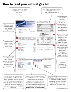

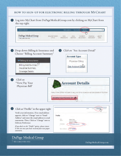

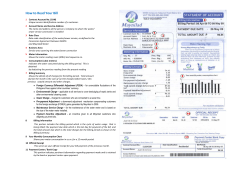
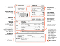


© Copyright 2026