
The Role of Geographical Context in Building Geodemographic
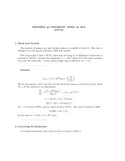
The Role of Geographical Context in Building Geodemographic Classifications Alexandros Alexiou Alex Singleton Dept. of Geography and Planning University of Liverpool 23rd GIS Research UK conference, Leeds, April 2015 Summary Introduction to Geodemographic Classifications Research Outline Methodology and Data Case studies Results and Discussion SCHOOL OF ENVIRONMENTAL SCIENCES 23rd GISRUK, Leeds, April 2015 Introduction A Geodemographic Classification (GC) is a data reduction technique that aims to generate through spatial profiling, clusters of populations that share similarities across multiple socio-economic and build environment attributes. Their composition differs based on the intended stakeholders’ perspective as well as the skills, experience and available data of the creator. Webber, 1977: pragmatic strategy; what is deemed to work and what is required, alongside some degree of empirical evaluation. Among the conventional classification systems : Proprietary classifications primarily designed to describe consumption patterns. Databases are populated not only with census data but compiled from large consumer databases such as credit checking histories, product registrations and private surveys. MOSAIC (Experian), ACORN (CACI), P2 People and Places (BD), Claritas (PRiZM) and EuroDirect (CAMEO). Public/Open Classifications: ONS Output Area Classification (OAC) 2001 and 2011. Similar products have also been created in academia. SCHOOL OF ENVIRONMENTAL SCIENCES 23rd GISRUK, Leeds, April 2015 Introduction Geodemographic classifications create a typology that is usually presented as a hierarchy; clusters produce varying tiers of aggregated areas. Cluster names are described usually through pen portraits. An example from the 2011 OAC: 1 – Rural residents 2 – Cosmopolitans 5a – Urban professionals and families 3 – Ethnicity central 4 – Multicultural metropolitans 5 – Urbanites 6 – Suburbanites 7 – Constrained city dwellers 5b – Ageing urban living 8 – Hard-pressed living 5a1 – White professionals 5a2 – Multi-ethnic professionals with families 5a3 – Families in terraces and flats 5b1 – Delayed retirement 5b2 – Communal retirement 5b3 – Self-sufficient retirement A top-down approach includes the creation of larger groups that are subsequently divided into smaller sub-groups. E.g. for the 2001 OAC, 7 super-groups split into 21 groups and further into 52 sub-groups. A bottom-up approach includes the creation of numerous smaller groups, aggregated based on their similarities into larger groups (typically with hierarchical algorithms such as Ward’s clustering criterion). Common clustering techniques used as classifiers: K-means clustering Self-Organizing Maps (SOM) Fuzzy logic algorithms or “soft” classifiers SCHOOL OF ENVIRONMENTAL SCIENCES 23rd GISRUK, Leeds, April 2015 Research Outline Main research question: Can conventional national classifications be applied locally with satisfactory results? If so, to what extent? what is the degree of differentiation? How can this differentiation be measured effectively? Rationale: Conventional national classifications may not account for local socio-spatial patterns, increasing the risk of mistargeting when applied locally. National aggregations sweep away contextual differences between proximal zones. Researchers without the necessary expertise may find it difficult to produce specificpurpose GCs ad hoc. General-purpose classifications are more convenient to use. Such debate is long withstanding, originating in the earliest of UK classifications (see Openshaw, Cullingford and Gillard, 1980 and Webber, 1980). SCHOOL OF ENVIRONMENTAL SCIENCES 23rd GISRUK, Leeds, April 2015 Methodology and Data This research uses a set of fixed input attributes for Output Area zonal geography to build classifications with different geographic context. For this purpose, a number of geographic contexts are considered (local, regional, national) to demonstrate the impact on final classification outcome when input variables are kept constant. In order to demonstrate how much output classifications differ, we perform an analysis of the sets of classifications for Liverpool, Manchester and Leeds. Creation: Initial 60+ Census 2011 Variables from Demographic, Housing and Economic Activity attributes. Output Area aggregation level for England (>170.000 neighbourhoods). K-Means Clustering (Hartigan & Wong, 1979), single hierarchy (Supergroup Level). Analysis carried out using the R software. SCHOOL OF ENVIRONMENTAL SCIENCES 23rd GISRUK, Leeds, April 2015 Methodology and Data K-Means Input Dataset Variable formatting: Obtaining ratios per areal unit Percentages Standardised by group where xa,i is the attribute value i of area a and Pa is the population of reference (denominator) of area a, i.e. total population, number of households, etc. where xa,i is the attribute value i of area a, rN,g is the observed national ratio N for group g and Pa,i is the population of group g in area a. “Unfit” data: Variable distribution and correlation checks. Normalisation using Box-Cox Transformation: Normalisation Transformation The power λ achieves the best normalization and can be estimated algorithmically. Box – Cox Standardisation (for all three geographic scales seperately): Variable Scaling Z-Score Scaling SCHOOL OF ENVIRONMENTAL SCIENCES where xa,i is the attribute value i of area a, μS is the mean and σS is the standard deviation of the set of observations S. 23rd GISRUK, Leeds, April 2015 Methodology and Data Final Dataset with Variable Definition: 2011 Census (ONS) V1 V2 V3 V4 V5 V6 V7 V8 V9 V10 V11 V12 V13 V14 V15 V16 V17 V18 V19 V20 V21 V22 V23 V24 V25 V26 V27 V28 V29 V30 V31 V32 V33 Demographic Age0_4 Age5_14 Age15_24 Age45_64 Age65_ Eth_Arab Eth_Black Eth_Asian Mar_Single Housing Density Ten_Rent Ten_Social House_Share House_Flat CeH_No Economic Activity EA_Part EA_Unemp EA_Stud Edu_Low Edu_HE NS_Manager NS_Semi Ind_Agr Ind_Man Ind_Sales Ind_Tech Ind_Adm Ind_Art Travel behavior Car_0 Car_1 Car_3 Tr_Public Tr_Foot Percentage of resident population aged 0–4 years Percentage of resident population aged 5–14 years Percentage of resident population aged 15-24 years Percentage of resident population aged 45–64 years Percentage of resident population aged 65 or more years Percentage of people identifying as Arab Percentage of people identifying as black African, black Caribbean or other black Percentage of people identifying as Indian, Pakistani, Bangladeshi, Chinese or Other Asian Percentage of population over 16 years who are single Number of people per hectare Percentage of households that are private sector rented accommodation Percentage of households that are public sector rented accommodation Percentages of households that are shared accommodation Percentage of households which are flats Percentage of occupied household spaces without central heating Percentage of household representatives who are working part-time Percentage of household representatives who are unemployed Percentage of household representatives who are students Percentage of people over 16 years with some qualifications but not a HE qualification Percentage of people over 16 years for which the highest level of qualification is level 4 qualifications and above Percentage of household reference persons in higher managerial, administrative and professional occupations Percentage of household reference persons in intermediate occupations Percentage of population aged 16-74 who work in the A, B and C industry sector Percentage of population aged 16-74 who work in the D, E and F industry sector Percentage of population aged 16-74 who work in the G, H and I industry sector Percentage of population aged 16-74 who work in the K, L and M industry sector Percentage of population aged 16-74 who work in the N, O, P, Q, T, and U industry sector Percentage of population aged 16-74 who work in the R and S industry sector Percentage of households with no car Percentage of households with 1 car Percentage of households with 3 or more cars Percentage of population aged 16-74 who travel to work by public transport Percentage of population aged 16-74 who travel to work on foot or by bicycle SCHOOL OF ENVIRONMENTAL SCIENCES 23rd GISRUK, Leeds, April 2015 Methodology and Data Currently there is no best practice to compare two different sets of classifications in order to find “best fits” between clusters (cluster IDs are assigned randomly): Two sources of cluster assignment variance: Even if they derive from the same observations set S, a classification for a set of local observations L compared with a national classification derived form S will produce dissimilar cluster assignments. Standardisation (for different geographical contexts, the mean μ and standard deviation σ changes) Clustering process We explore and illustrate the variation with a number of methods: 1. Plotting the Cluster Mean Centres (attribute means) so we can assess the nature of the cluster (pen-portraits). 2. Contingency Tables: cross-tabulating the cluster distribution frequencies. 3. Mapping our results. SCHOOL OF ENVIRONMENTAL SCIENCES 23rd GISRUK, Leeds, April 2015 Case Studies We compare 3 sets of classifications, one set for each case study, that were built using the same data set: Geographic area Local Classification Regional Classification National Classification Liverpool Liverpool Local Authority North West England Manchester Greater Manchester Area North West England Leeds Leeds Local Authority Yorkshire and the Humber England We compare outcomes based on k-means algorithm for 7 clusters: 1. Radial plots to assess “attribute fit”. 2. Cross-tabulation to assess “geographic fit”. SCHOOL OF ENVIRONMENTAL SCIENCES 23rd GISRUK, Leeds, April 2015 Case Studies Constructing Pen Portraits SCHOOL OF ENVIRONMENTAL SCIENCES 23rd GISRUK, Leeds, April 2015 Case Studies - Liverpool Cross-Tabulation vs. Radial Plots SCHOOL OF ENVIRONMENTAL SCIENCES Liverpool Cluster Name OA Amount NW Cluster NW OA Amount Urban Professionals Retired Communities Student Living Striving Ethnic Workers Suburban Living Hard-Pressed Families Young Cosmopolitans Sum / Mean 332 185 81 171 306 381 128 1584 3 2 5 7 4 6 1 203 0 81 134 52 352 36 858 Liverpool Cluster Name OA Amount National Cluster Urban Professionals Retired Communities Student Living Striving Ethnic Workers Suburban Living Hard-Pressed Families Young Cosmopolitans Sum / Mean 332 185 81 171 306 381 128 1584 3 2 5 7 4 6 1 Cluster Similarity 61% 0% 100% 78% 17% 92% 28% 54.2% National Cluster OA Similarity Amount 214 64% 9 5% 81 100% 126 74% 103 34% 381 100% 36 28% 950 60.0% 23rd GISRUK, Leeds, April 2015 Case Studies - Liverpool Cross-Tabulation vs. Radial Plots SCHOOL OF ENVIRONMENTAL SCIENCES Liverpool Cluster Name OA Amount NW Cluster NW OA Amount Urban Professionals Retired Communities Student Living Striving Ethnic Workers Suburban Living Hard-Pressed Families Young Cosmopolitans Sum / Mean 332 185 81 171 306 381 128 1584 3 2 5 7 4 6 1 203 0 81 134 52 352 36 858 Liverpool Cluster Name OA Amount National Cluster Urban Professionals Retired Communities Student Living Striving Ethnic Workers Suburban Living Hard-Pressed Families Young Cosmopolitans Sum / Mean 332 185 81 171 306 381 128 1584 3 2 5 7 4 6 1 Cluster Similarity 61% 0% 100% 78% 17% 92% 28% 54.2% National Cluster OA Similarity Amount 214 64% 9 5% 81 100% 126 74% 103 34% 381 100% 36 28% 950 60.0% 23rd GISRUK, Leeds, April 2015 Case Studies - Liverpool Cross-Tabulation vs. Radial Plots Liverpool Cluster Name OA Amount NW Cluster NW OA Amount Urban Professionals Retired Communities Student Living Striving Ethnic Workers Suburban Living Hard-Pressed Families Young Cosmopolitans Sum / Mean 332 185 81 171 306 381 128 1584 7 3 1 5 6 4 2 203 0 81 134 52 352 36 858 Liverpool Cluster Name Urban Professionals Retired Communities Student Living Striving Ethnic Workers Suburban Living Hard-Pressed Families Young Cosmopolitans Sum / Mean SCHOOL OF ENVIRONMENTAL SCIENCES Cluster Similarity 61% 0% 100% 78% 17% 92% 28% 54.2% OA National Nat. OA Cluster Amount Cluster Amount Similarity 332 3 214 64% 185 2 9 5% 81 5 81 100% 171 7 126 74% 306 4 103 34% 381 6 381 100% 128 1 36 28% 1584 950 60.0% 23rd GISRUK, Leeds, April 2015 Case Studies – G. Manchester Cross-Tabulation vs. Radial Plots G. Manchester Cluster Name Asian Communities Age0_4 Ind_Art2.5 Age5_14 Ind_Adm Age15_24 Ind_Tech Age45_64 2 Ind_Sales Age65_ 1.5 1 Ind_Man Car_0 0.5 Ind_Agr Car_1 0 -0.5 Tr_Foot Car_3 -1 Tr_Public CeH_No -1.5 Mar_Married Density Mar_Single EA_Part Ten_Social EA_Unemp Ten_Rent NS_Semi NS_Manager House_Flat Edu_HE EA_Stud Eth_Asian Eth_Black Eth_Arab Edu_Low SCHOOL OF ENVIRONMENTAL SCIENCES OA Amount Urban Professionals Asian Communities 2255 546 Student Living Striving Ethnic Workers Suburban Living Hard-Pressed Families Young Cosmopolitans Sum / Mean 360 864 2202 1638 819 8684 NW Cluster G Retired Communities A E F D B NW OA Amount Cluster Similarity 1 1 0.0% 0.2% 359 724 945 1389 764 4183 99.7% 83.8% 42.9% 84.8% 93.3% 48.2% G. Manchester Cluster Name Urban Professionals Asian Communities OA National Nat. OA Cluster Amount Cluster Amount Similarity 2255 B 1398 62.0% 546 Retired 0 0.0% Communities Student Living 360 G 287 79.7% Striving Ethnic Workers 864 F 547 63.3% Suburban Living 2202 E 1189 54.0% Hard-Pressed Families 1638 A 1614 98.5% Young Cosmopolitans 819 D 293 35.8% Sum / Mean 8684 5328 61.4% 23rd GISRUK, Leeds, April 2015 Case Studies - Leeds Cross-Tabulation vs. Radial Plots Leeds Cluster Name Urban Professionals Young & Single “Techies” Student Living Striving Ethnic Workers Suburban Living Hard-Pressed Families Young Cosmopolitans Sum / Mean Leeds Cluster Name Urban Professionals Young & Single "Techies" Student Living Striving Ethnic Workers Suburban Living Hard-Pressed Families Young Cosmopolitans Sum / Mean SCHOOL OF ENVIRONMENTAL SCIENCES OA Amount 682 112 116 373 340 569 351 2543 YH Cluster C Retired Communities G D E A B YH OA Amount Cluster Similarity 461 0 67.6% 0.0% 116 352 300 301 340 1870 100.0% 94.4% 88.2% 52.9% 96.9% 73.5% OA National Cluster Nat. OA Cluster Amount Amount Similarity 682 G 342 50.1% Retired 112 Communities 0 0.0% 116 D 115 99.1% 373 F 253 67.8% 340 B 298 87.6% 569 E 470 82.6% 351 A 121 34.5% 2543 1599 62.9% 23rd GISRUK, Leeds, April 2015 Results and Discussion Geographic Sensitivity of geodemographic classifications is very difficult to assess, given the complexity of the problem. Some remarks: Cluster Comparison - Hard-Pressed Households The notions of attribute fit and geographic fit are central to comparisons. Attribute means do provide a basis for correlation between cluster pairs, however they do not account for the magnitude of deviation of the OA attribute values from the mean. Between geographic scales, formed clusters can be completely different in nature, making comparisons inconclusive. Policy implications: In-between classification comparisons: Small differentiation in attributes can demonstrate central tendencies of the local populations. However actual socio-spatial patterns can in fact be very different. Age0_4 Ind_Art1.5 Age5_14 Ind_Adm Age15_24 Ind_Tech Age45_64 1 Ind_Sales Age65_ Ind_Man 0.5 Car_0 0 Ind_Agr Car_1 -0.5 Tr_Foot Car_3 -1 Tr_Public CeH_No -1.5 Mar_Married Density Mar_Single EA_Part Ten_Social EA_Unemp Ten_Rent NS_Semi NS_Manager House_Flat Edu_HE Liverpool EA_Stud Eth_Asian Eth_Black Eth_Arab Edu_Low Manchester Leeds When assessing spatial policies, upper hierarchies (i.e. Supergroup Level) from national classifications may not be suitable as they can produce misleading results. SCHOOL OF ENVIRONMENTAL SCIENCES 23rd GISRUK, Leeds, April 2015 Results and Discussion Methodological Implications: Standardising attributes directly affects cluster formation. Clusters at national scales appear more homogenous due to reduced absolutes distances. I.e. for k = 7, the total variation lost (smoothed out) has a magnitude of ~ 9%. A key research should focus on whether there are specific geographical contexts that maximise clustering efficiency to local variation, and how unique clusters can be handled. Administrative boundaries do not necessarily reflect the actual organisation of communities. For instance calculating geographic boundaries in non-Euclidian space. SCHOOL OF ENVIRONMENTAL SCIENCES 23rd GISRUK, Leeds, April 2015 Results and Discussion Future research and preliminary results (benchmark geographic boundaries) We use the angular similarity measure to compare cluster attribute means: Benchmark results: LA (Local Authority) Classification vs. National Classification. Standardised attributes per LA. The aim is to produce geographic boundaries that maximize local efficiency, other than the arbitrary administrative boundaries. Such boundaries can be used in any research regarding population dynamics (e.g. retail analysis) and can be made publicly available easily. SCHOOL OF ENVIRONMENTAL SCIENCES 23rd GISRUK, Leeds, April 2015 Thank you for your time [email protected] https://speakerdeck.com/dblalex Acknowledgements: This work is funded as part of an ESRC PhD studentship and in collaboration with the Office for National Statistics North West Doctoral Training Centre


© Copyright 2026