Brief announcements
Distributed Systems & Control
1
fourth homework will be
posted next week and
will contain material
spanning multiple
lectures
2
projects are posted &
we have received the
group info
Advanced Topics in Control 2015
Lecture 9: Time-varying averaging
⇒ group/project
assignment posted online
⇒ start off working
1 / 34
2 / 34
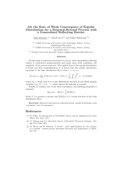
A teaser
Continuous-time example:
−1 102
x˙ =
x
0 −1
what info do you get from the
spectrum of a non-symmetric
matrix anyways (?) . . .
x ’ = − x − 100 y
y’=−y
recap: convergence factors
+2 x2
2
1.5
1
(chapter 8)
0.5
y
0
−0.5
−1
−1.5
2
−2
−40
3 / 34
40
−30
−20
−10
0
x
10
20
30
x1
+40
40
4 / 34
The disagreement vector & its dynamics
Convergence factors & solution bounds
Theorem: Let A be doubly-stochastic and primitive.
setup: A is doubly-stochastic & primitive
1
⇒ convergence of x(` + 1) = Ax(`) to xfinal = average(x0 ) · 1
disagreement vector:
The convergence factors of A satisfy
T
rstep (A) = A − 1n 1n /n ,
2
δ(`) = x(`) − average(x0 ) · 1
rasym (A) = ρess (A) = ρ(A − 1n 1T
n /n) < 1,
⇒ disagreement dynamics: δ(` + 1) = A − 11T /n δ(`)
Moreover, rasym (A) ≤ rstep (A), and rstep (A) = rasym (A) if A = AT .
⇒ orthogonality: δ(`) ⊥ 1 for all ` ∈ Z≥0
2
⇒ stability: ρ A − 11T /n < 1 ⇔ A is primitive
For any initial condition,
kδ(`)k2 ≤ rstep (A)` kδ0 k2 ,
kδ(`)k2 ≤ Cε (rasym (A) + ε)` kδ0 k2 ,
per-step conv. factor: rstep (A) = supδ(`)6=O kδ(` + 1)k2 /kδ(`)k2
asymptotic conv. factor: rasym (A)` = supδ0 6=O lim kδ(` + 1)k2 /kδ0 k2
`→∞
where ε > 0 is an arbitrarily small constant and Cε is a sufficiently
large constant independent of x0 .
5 / 34
6 / 34
the general case of a
strongly connected graph is
almost perfectly identical . . .
the continuous-time case is
perfectly identical . . .
7 / 34
8 / 34
Organization of today’s lecture
Convergence rates
& scalability
Time-varying
averaging
(Chapter 9)
(Chapter 10)
bounds are for worst-case
initial values supδ06=O . . .
what about average
performance ?
9 / 34
10 / 34
Average performance for random initial conditions
setup: A is doubly-stochastic & primitive
⇒ convergence of x(` + 1) = Ax(`) to xfinal = average(x0 ) · 1
random initial conditions x0 with E x0 = 0 and E x0 x0T = I
disagreement dynamics: δ(` + 1) = A − 11T /n δ(`)
with E δ0 = 0 and E δ0 δ0T = I − 11T /n
1
N
X
λ∈spec(A)\{1}
PT
kδ(`)k22
1 − λ2(T −1) T →∞ 1
−−−−→
1 − λ2
N
X
Theorem: If A is symmetric, then
JT (A) =
1
N
`=0 E
linear quadratic (LQ) cost JT (A) =
discussion on board
λ∈spec(A)\{1}
1
.
1 − λ2
11 / 34
12 / 34
A case study for the ring graph

0
1
2N-1
An,k
N-1
N





=





1 − 2k
k
0
..
.
0
k
[R. Carli, F. Garin, & S. Zampieri, ’09]

kProposition
0 1 (LQ
· · · cost asymptotics):
0
k
Given {Pn }n≥δ a
 with p(z , . . . , z ),
..
..
Cayley
or
a
grid
matrix
family
associated
1
d
.
.
1 − 2k
k
0 
on d) such that:
there exist Cd , Cd′ .>. 0 (depending
only

.
..
.. 
.
.
k
1 − 2k
,
• if d = 1,
′
..
..
..
..
C1 N ;
.
.
. J∆ (Pn )0 ≤ 
.C1 N ≤


..
..
• . if d = 2,.
k
1 − 2k
k 
0
···
where k ∈ [0, 1/2[• if d ≥ 3,
with 2N vertices and reflection axis corresponding to the map
− l, used in the construction of a line with N vertices.
⇒ last exercise: λi = 2k cos 2π(i−1)
n
0
k
1 − 2k
C2 log N ≤ J∆ (Pn ) ≤ C2′ log N ;
time-varying
averaging
algorithms
Cd ≤ J∆ (Pn ) ≤ Cd′ .
!
To give a better understanding of the above Theorem,
me coefficients that Pn associates to edges of the we propose an example illustrating
an interestig comparison
2 k 1 +ofOthe1 functional cost J and of the
torus. ⇒ worst-case convergence: ρess (An,k
between
the4π
behavior
)≈1−
∆
2
4
n
n
refer to the above construction of a family of essential spectral ρess as n → ∞ of a particular sequence
of Cayley graphs.
n }n≥δ with the short name ‘grid matrix family
n We owill see how the evaluation of the
with p(z1⇒
, . . .average
, zd )’.
performance
of
performance: JT (A) ≈ const. · max n1the
, √1 average consensus algorithms, in the
Prop. 3.2], we can find the eigenvalues of P n :
asymptotic regime n T→ ∞, is strictly related to the choice
13 / 34
14 / 34
of the functional cost.
i π h1
i π hd
),
h ∈ Vn .
h = p(e n , . . . , e n
Example 1: Consider the sequence of Cayley matrices
3
{P
geometric graphs
% n } built as follows. For each n, let G = Zn and let S =
(0, 0, 0),&(1, 0, 0), (0, 1, 0), (0, 0, 1), (−1, 0, 0), (0, −1, 0),
om geometric graph is a random undirected graph
(0, 0, −1) . Moreover let π(g) = 17 for all g ∈ S. It is well
Averaging
shared communication
channel I
Averaging with shared communication channel II
bounded
region, e.g.,with
the d-dimensional
unitary
known (see [5]) that, in this case,
It is generated by
C
Protocol:
a communication
Gshared-comm
vertices
at random, Given
uniformly
and independently
ρess (Pn ) ≥ 1 − 3
Protocol: Each node has a different
N
Gshared-comm
digraph
he region,
and Gshared-comm , at each
clock
&
there
is
no
common
schedule.
3
4
where
C
is
a
constant
independent
from
the
topology
of
the
ting twocommunication
vertices if and only
if
the
euclidean
disround, only one node
3
4
graphs. From the above inequality it turns out that, Suppose
if we
that messages are safely
etween can
themtransmit
is at most to
a pre-assigned
threshold r. over
all its out-neighbors
consider as functional cost the asymptotic covergence delivered
factor
even if transmitting & receiving
m geometric
graph was
in [13]node
a common
bus first
and introduced
every receiving
defined
in
(4),
then
the
performance
of
the
average
consensus
en deeply studied under a communications and
agents are not synchronized. Each time
1
2
will implement a single averaging step.
drasti1
2
-theoretic point of view in [14]. It has recently algorithms associated to the sequence {Pn } degrades an
agent wakes up, the available
cally
as
n
→
∞.
Instead,
Proposition
1
guarantees
the
exislarge interest in many applications; particularly
′
′
information
from its neighbors varies.
successfully used to model wireless communica- tence of constants C3+and C13 such that C3 ≤ J∆ (Pn ) ≤ C3
Update: j receives the message from i for
& all
implements
x
:=
(x
+x
)
j
n.
!
j
2 i
n Section IV-B, given a random geometric graph
Proposition
2
(Quadratic
estimation
error
asymptotics):
e will associate to it a doubly stochastic matrix P
Update: At an iteration instant for agent i, assuming agent i has new
ing to the Metropolis weights rule [29]; precisely, Given {Pn }n≥δ a Cayley or a grid matrix family associated
′
Round-robin schedule: i talks only atwith
times
i,
n
+
i,
2n
+
i,
.
.
.
,
k
·
n
+
i
p(z1 , . . . , zd ), there exist constants c0 = c0 messages/information
= 1,
from agents i1 , . . . , im , agent i will implement:
es the element of P in the i-th row and in the j-th
′
′
c
,
.
.
.
,
c
,
c
,
.
.
.
,
c
>
0
and
k
∈
(0,
1)
such
that
1
d
1
d
will have
3
4
3
4
3
4
3
4
1
1
⎧
'
1
1 cl
1 c′l
xi+ := m+1
xi + m+1
(xi1 + · · · + xim )
t
if
(i,
j)
∈
E
⎨ 1+max{d
max
≤
J
(P
,
t)
≤
k
+
,d
}
e
n
$ i j
d−l
d−l
l/2
l/2
l=0,...,d n
n
t
t
1 − 1(i,k) ∈ E\{(i,i)}
2 Pik
1 if i = j 2
1
2
1
2
l=0,...,d
⎩
0
otherwise
time = 1, 5, 9, . . . time = 2, 6, 10, . . . time = 3, 7, 11, . . . time = 4, 8, 12, . . .
!
(structure? convergence?)
Corollary 1: Given {Pn }n≥δ a Cayley or a grid Update
matrix sequence: x(` + 1) = A(`)x(`)
|Ni \{(i, i)} | with Ni = {j ∈ V | (i, j) ∈ E}. In
with p(z1 , . . . , zd ), there exists constants
Update
sequence:
1) =
An−1family
· · · A1associated
x(1)
the weight
on each
edge is onex(n
over+one
plusAnthe
16 / 34
15 / 34
ee at its two incident vertices, and the self-weights n0 ∈ N, k1 , k2 > 0 such that, for all n ≥ n0 ,
(
)
(
)
+ (1 − 2k) for i ∈ {1, . . . , n}
(chapter 10)
The scalar time-varying iteration x(` + 1) = a(`)x(`)
3
x(l+1) = exp(−1/(l+1)2)*x(l)
y(l+1) = exp(−1/(l+1))*y(l)
2.5
2
1.5
warm-up
1
0.5
0
0
5
10
15
20
25
A necessary and sufficient condition convergence is
17 / 34
30
.
18 / 34
The matrix case x(` + 1) = A(`)x(`)
solution is x(`) = Π`−1
k=1 A(k)x0 = A(` − 1) · A(`) · · · A(1) · x0
condition(?) if for each ` ∈ Z≥0 we have ρ(A(`)) < 1, then
.
1
1
1
0
2
puzzling example with ρ(Ai ) < 1: A1 =
and A2 =
0 0
1 0
exp(−1/(` + 1)α )
1 − exp(−1/(` + 1)α )
averaging: A(`) =
1 − exp(−1/(` + 1)α )
exp(−1/(` + 1)α )
2
discrete averaging algorithms
2
1.9
1.8
1.7
1.6
1.5
1.4
1.3
1.2
1.1
1
0
1
2
3
4
5
6
7
8
9
10
19 / 34
20 / 34
Consensus for time-varying algorithms
Theorem: Let {A(`)}`∈Z≥0 be a sequence of row-stochastic matrices with
associated digraphs {G (`)}`∈Z≥0 . Assume that
(A1) each digraph G (`) has a self-loop at each node;
(A2) each non-zero edge weight aij (`), including the self-loops weights
aii (`), is larger than a constant ε > 0; and
point-wise convergence on board
(A3) there exists a duration δ ∈ N such that, for all times ` ∈ Z≥0 , the
digraph G (`) ∪ · · · ∪ G (` + δ − 1) contains a globally reachable node.
Then
1
2
the solution to x(` + 1) = A(`)x(`) converges exp. fast to w T x0 1,
where w ∈ Rn≥0 is normalized to w1 + · · · + wn = 1; and
if additionally each matrix in the sequence is doubly-stochastic, then
w = n1 1n so that lim`→∞ x(`) = average(x0 )1.
22 / 34
21 / 34
Consensus for symmetric time-varying algorithms
Theorem: Let {A(`)}`∈Z≥0 be a sequence of symmetric row-stochastic
matrices with associated undirected graphs {G (`)}`∈Z≥0 . Assume that
(A1) each digraph G (`) has a self-loop at each node;
(A2) each non-zero edge weight aij (`), including the self-loops weights
aii (`), is larger than a constant ε > 0; and
proof ideas on board
(A4) for all ` ∈ Z≥0 , the graph ∪τ ≥` G (τ ) is connected.
Then the solution to x(` + 1) = A(`)x(`) converges exponentially fast to
average(x0 )1.
Compare to previous assumption (A3):
there exists a duration δ ∈ N such that, for all times ` ∈ Z≥0 , the digraph
G (`) ∪ · · · ∪ G (` + δ − 1) contains a globally reachable node.
23 / 34
24 / 34
Uniform connectivity is required for asymmetric matrices
Initialize a group of n = 3 agents to
x1 < −1,
x2 < −1,
x3 > +1.
x1 > +1,
x2 < −1,
x3 > +1.
x2 < −1,
x3 < −1.
x2 > +1,
x3 < −1.
Step 1: perform x1+ := (x1 + x3 )/2, x2+ := x2 , x3+ := x3 δ1 times until
Step 2: perform x1+ := x1 , x2+ := x2 , x3+ := (x2 + x3 )/2 δ2 times until
x1 > +1,
observations on board
Step 3: perform x1+ := x1 , x2+ := (x1 + x2 )/2, x3+ := x3 a δ3 times until
x1 > +1,
And repeat this process.
1
2
1
∪
3
step 1
2
3
step 2
1
∪
2
3
step 3
1
=
2
union
3
25 / 34
26 / 34
Motivation I: flocking behavior
or
continuous averaging algorithms


(θj − θi ),
θ˙i = 12 (θj1 − θi ) + 12 (θj2 − θi ),

1
1
m (θj1 − θi ) + · · · + m (θjm − θi ),
if one neighbor at time t
if two neighbors at time t
if m neighbors at time t
θ˙i = average {θj , j ∈ N out(t) (i)} − θi
or
θ˙ = −L(t)θ
27 / 34
28 / 34
Motivation II: coupled oscillators
P
Mi θ¨i + Di θ˙i = Ωi − j Kij sin(θi − θj )
Ω1
Ω2
• inertia constants Mi > 0
• viscous damping Di > 0
• external torques Ωi ∈ R
• spring constants Kij ≥ 0
For Di = 1, Mi Di , and Ωi = 0:
⇔
⇒
⇒
Ω3
warm-up example
P
θ˙i = − j Kij sin(θi −θj )
P
θ˙i (t) = − j aij (t)(θi (t) − θj (t)) with aij (t) = Kij sinc(θi (t) − θj (t))
if |θi (t) − θj (t)| < π for all {i, j} ∈ E and for all t ≥ 0, then aij (t) > 0
coupled oscillator network reduced to Laplacian flow θ˙ = −L(t)θ
29 / 34
30 / 34
Time-varying algorithms — connected point-wise in time
Consensus for time-varying algorithms
Theorem: Let t 7→ L(t) = L(t)T be a time-varying Laplacian matrix with
associated time-varying digraph t 7→ G (t), t ∈ R≥0 . Assume
Theorem: Let t 7→ A(t) be a time-varying adjacency matrix with
associated time-varying digraph t 7→ G (t), t ∈ R≥0 . Assume
[Moreau, 04]
(A1) each non-zero edge weight aij (t) is larger than a constant ε > 0,
(A1) each non-zero edge weight aij (t) is larger than a constant ε > 0,
(A2) for all t ∈ R≥0 , the digraph associated to the symmetric Laplacian
matrix L(t) is undirected and connected.
(A2) there exists a duration T > 0 such that, for all t ∈ R≥0 , the digraph
associated to the adjancency matrix
Z
Then the solution to x(t)
˙
= −L(t)x(t) converges exp. to average(x0 )1.
t+T
A(τ )dτ
t
Limitations of quadratic Lyapunov functions: Let L be a Laplacian
associated with a weighted digraph G . The following are equivalent:
1
L + LT is negative semi-definite;
2
L has zero column sums, that is, G is weight-balanced;
3
4
the sum of squares function V (δ) = kδk2 is strictly decreasing; and
every convex function V (x) invariant under coordinate permutations
is non-increasing along the trajectories of x˙ = −Lx.
31 / 34
contains a globally reachable node.
Then
1
2
the solution
to x(t)
˙
= −L(t)x(t) converges exponentially fast to
T
w x0 1, where w ∈ Rn≥0 is normalized to w1 + · · · + wn = 1; and
if additionally, the 1T L(t) = OT for almost all times t, then w = n1 1
so that limt→∞ x(t) = average(x0 )1.
32 / 34
Symmetric time-varying consensus algorithms
[Hendrickx et al. ’13]
Theorem: Let t 7→ A(t) be a time-varying symmetric adjacency matrix.
Consider an associated undirected graph G = (V , E ), t ∈ R≥0 that has an
edge (i, j) ∈ E if
Z ∞
aij (τ )dτ
0
is divergent. Assume that
Reading assignment (lecture notes):
Extra notes on average performance
Chapter 10: Time-varying averaging
(A1) each non-zero edge weight aij (t) is larger than a constant ε > 0,
(A2) the graph G is connected.
Exercise session (Friday):
Then the solution to x(t)
˙
= −L(t)x(t) converges exponentially fast to
average(x0 )1.
review of take-home messages
examples & additional facts
Compare to previous assumption (A3): there exists a duration T > 0
such that, for all t ∈ R≥0 , the digraph associated to the adjancency matrix
R t+T
A(τ )dτ contains a globally reachable node.
t
33 / 34
exercises & illustrations
34 / 34