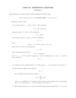
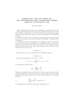
Generalized Tensor Total Variation Minimization for Visual Data Recovery∗
Xiaojie Guo1 and Yi Ma2
1
State Key Laboratory of Information Security, IIE, CAS, Beijing, 100093, China
2
School of Information Science and Technology, ShanghaiTech University, Shanghai, 200031, China
[email protected] | [email protected]
N ∈ RD1 ×D2 ×···×Dn by solving the following problem:
Abstract
min Φ(T ) + λΨ(N ) s. t. PΩ (O) = PΩ (T + N ), (1)
In this paper, we propose a definition of Generalized
Tensor Total Variation norm (GTV) that considers both the
inhomogeneity and the multi-directionality of responses to
derivative-like filters. More specifically, the inhomogeneity
simultaneously preserves high-frequency signals and suppresses noises, while the multi-directionality ensures that,
for an entry in a tensor, more information from its neighbors is taken into account. To effectively and efficiently seek
the solution of the GTV minimization problem, we design a
novel Augmented Lagrange Multiplier based algorithm, the
convergence of which is theoretically guaranteed. Experiments are conducted to demonstrate the superior performance of our method over the state of the art alternatives
on classic visual data recovery applications including completion and denoising.
T ,N
where PΩ (·) is the orthogonal projection operator on the
support Ω ∈ {0, 1}D1 ×D2 ×···×Dn that indicates which elements are observed. Ψ(N ) is a penalty with respect to
noise, which usually adopts `1 norm that is optimal for
Laplacian noise, or Frobenius norm for Gaussian noise. The
non-negative parameter λ provides a trade-off between the
noise sensitivity and closeness to the observed signal. And
Φ(T ) stands for the assumption to make the ill-posed tensor recovery problem well-defined. In literature, there are
mainly two lines about the assumption, i.e. the low rankness and the low total variation.
The low-rank nature of visual data, say Φ(T ) :=
rank(T ), has been focus of considerable research in past
years, the effectiveness of which has been witnessed by numerous applications, such as image colorization [15], rectification [18], denoising [5], depth enhancement [10] and
subspace learning [13]. As for the tensor recovery task,
specifically, Liu et al. [9] first introduce the trace norm
for tensors to achieve the goal. More recently, Wang et
al. [14] simultaneously impose the low rank prior and the
spatial-temporal consistency for completing videos. Zhang
et al. [17] design a hybrid singular value thresholding strategy for enhancing the low rankness of the underlying tensors. Although these methods produce very promising results on the visual data with strong global structure, the
performance of which would degrade on general tensors
of visual data. To mitigate the over-strict constraint, [3]
uses factor priors to simultaneously decompose and complete tensors, which follows the tensor factorization framework proposed in [11]. Actually, [3] instead enforces the
low rank constraint on the low dimensional representation
(sub-manifold) of the data.
Alternatively, the visual tensor to be recovered should
be piece-wise smooth, that is Φ(T ) := kT kT V . In last
decades, the advances in matrix Total Variation (TV) minimization have demonstrated its significance as a theoretic
1. Introduction
In real data analysis applications, we often have to face
handling dirty observations, say incomplete or noisy data.
Recovering the missing or noise-free data from such observations thus becomes crucial to provide us more precise
information to refer to. Besides, compared to 1-D vectors
and 2-D matrices, the data encountered in real world applications is more likely to be high order, for instance a multispectral image is a 3-D tensor and a color video is a 4-D
tensor. This work concentrates on the problem of visual
data recovery, i.e. restoring tensors of visual data from polluted observations. However, without additional priors, the
problem is intractable as it usually has infinitely many solutions and thus, it is apparently impossible to identify which
of these candidate solutions is indeed the “correct” one.
Mathematically, under some assumptions, one would
want to recover a n-order tensor T ∈ RD1 ×D2 ×···×Dn from
an observation O ∈ RD1 ×D2 ×···×Dn in presence of noise
∗ This work was supported in part by the National Natural Science
Foundation of China (No. 61402467) and in part by the Excellent Young
Talent Programme through the Institute of Information Engineering, CAS.
1
foundation for this problem. The TV model was first introduced in [12] as a regularizer to remove noises and handle
proper edges in images. A variety of applications [2, 6] have
proven its great benefit. Although the TV norm has been
extensively studied for matrices, there is not much work
on tensors. Yang et al. [16] simply extend the TV norm
for matrices to higher-order tensors and design an efficient
algorithm to solve the optimization problem. But, it only
takes care of the variations along fibers (see the definition
below), and breaks the original problem into a set of 1-D
vector problems [4] to accelerate the procedure, which limits its flexibility (multi-directionality).
1.1. Notations and Tensor Basics
We first define the notations used in this paper. Lowercase letters (a, b, ...) mean scalars and bold lowercase letters (a, b, ...) vectors. Bold uppercase letters (A, B, ...)
stand for matrices. The vectorization operation of a matrix
vec(A) is to convert a matrix into a vector. For brevity, Aj
stands for the j th column of A. While bold calligraphic uppercase letters (A, B, ...) represent high order tensors. A ∈
RD1 ×D2 ×···×Dn denotes an n-order tensor, whose elements
are represented by ad1 ,d2 ,...,dn ∈ R, where 1 ≤ dk ≤ Dk
and 1 ≤ k ≤ n. ad1 ,...,dk−1 ,:,dk+1 ,...,dn ∈ RDk means the
mode-k fiber of A at {d1 , ..., dk−1 , dk+1 , ..., dn }, which is
the higher order analogue of matrix rows and columns.
The Frobenius, `1 and `0 qnorms of A are respecP
2
tively defined as kAkF :=
d1 ,d2 ,··· ,dn ad1 ,d2 ,...,dn ,
P
:=
kAk
d1 ,d2 ,··· ,dn |ad1 ,d2 ,...,dn | and kAk0
P 1 :=
a
=
6
0.
The
inner
product
of
two
d
,d
,...,d
1 2
n
d1 ,d2 ,··· ,dn
tensors
with identical size is computed as hA, Bi :=
P
d1 ,d2 ,··· ,dn ad1 ,d2 ,...,dn · bd1 ,d2 ,...,dn . A B means the
element-wise product of two tensors with same size. The
mode-k unfolding of A is to convert a tensor QA into
a matrix, i.e. unfold(A, k) = A[k] ∈ RDk × i6=k Di ,
while the mode-k folding reshapes A[k] back to A, say
fold(A[k] , k) = A. It is clear that, for any k, kAkF =
kA[k] kF , kAk1 = kA[k] k1 , kAk0 = kA[k] k0 , and
hA, Bi = hA[k] , B [k] i. Sω [A] represents the uniform
shrinkage operator on tensors, the definition of which
is that, for each element in A, Sω [ad1 ,d2 ,...,dn ] :=
sgn(ad1 ,d2 ,...,dn ) · max(|ad1 ,d2 ,...,dn | − ω, 0). More generally, the non-uniform shrinkage SW [A] extends the uniform one by performing the shrinkage on the elements of A
with thresholds given by corresponding entries of W.
1.2. Motivations of This Work
A natural extension of the TV norm for matrices to
higher-order tensors has the following shape [16]:
kT kT V := kf π2 ∗ [vec(T [1] )| vec(T [2] )|...| vec(T [n] )]kp ,
(2)
where k · kp can be either `1 norm corresponding to the
anisotropic tensor TV norm, or `2,1 the isotropic one. f π2 is
the derivative filter in the vertical (θ = π2 ) direction and ∗ is
the operator of convolution. It is obvious that the TV norms
for vectors and matrices are two examples of this definition.
However, in practical scenarios, this definition (2) is inadequate mainly due to the following limitations:
◦ The homogeneous penalty leads to the oversmoothness on high-frequency signal, such as
corners and edges in visual data, and creates heavy
staircase artifacts, which would significantly disturb
the perception of visual data.
◦ It only considers the variations along fibers, which
might miss important information in other directions.
Although the responses to multi-directional derivativelike filters can be approximately represented by the
gradients, the gap between them remains.
The above two limitations motivate us to propose a more
general tensor TV norm for boosting the performance on
the visual data recovery problem.
1.3. Contributions of This Work
The contributions of this work are summarized as:
• We propose a Generalized Tensor Total Variation norm
(GTV) concerning both the inhomogeneity and the
multi-directionality.
• We design an Augmented Lagrange Multiplier based
algorithm to efficiently and effectively seek the solution of the GTV minimization problem, the convergence of which is theoretically guaranteed.
• To demonstrate the efficacy and the superior performance of the proposed algorithm in comparison with
state-of-the-art alternatives, extensive experiments on
several visual data recovery tasks are conducted.
2. Methodology
2.1. Definition and Formulation
Suppose we have a matrix A ∈ RD1 ×D2 , the response of
A to a directional derivative-like filter fθ∗ can be computed
by fθ∗ ∗ A. The traditional TV norm takes into account
only the responses to derivative filters along fibers. In other
words, it potentially ignores important details from other directions. One may wonder if the multi-directional response
can be represented by the gradients. Indeed, for differentiable functions, the directional derivatives along some directions have an equivalent relationship with the gradients.
However, for tensors of visual data, this relationship no
longer holds as the differentiability is violated. Based on
this fact, we here propose a definition of the responses of a
matrix to m-directional derivative-like filters as follows:
Definition 1. (RMDF: Response to Multi-directional
Derivative-like Filters.) The response of a matrix to m
derivative-like filters in θm directions with weights βm is
defined as R(A, β) ∈ RD1 D2 ×m :=
β1 vec(fθ1 ∗ A)β2 vec(fθ2 ∗ A) · · · βm vec(fθm ∗ A) ,
where
= [β1 , β2 , · · · , βm ] with ∀j ∈ [1, ..., m] βj ≥ 0
Pβ
m
and j=1 βj = 1.
Another drawback of the traditional TV is its homogeneity to all elements in tensors, which favors piecewise constant solutions. This property would result in oversmoothing high-frequency signals and introducing staircase effects.
Intuitively, in visual data, the high-frequency signals should
be preserved to maintain the perceptual details, while the
low-frequency ones could be smoothed to suppress noises.
This intuition inspires us to differently treat the variations.
Considering both the multi-directionality and the inhomogeneity gives the definition of generalized tensor TV as:
Definition 2. (GTV: Generalized Tensor Total Variation
Norm.) The GTV norm of an n-order tensor A ∈
RD1 ×···×Dn is:
kAkGT V :=
n
X
αk kW k R(A[k] , β k )kp ,
k=1
where α = [α1 , ..., αk , ..., αn ] is the non-negative coefficient balancing
Pn the importance of k-mode matrices and
satisfying k=1 αk = 1, and p could be either 1 or 2, 1
corresponding to the anisotropic total variation (`1 ) and
theQ isotropic one (`2,1 ), respectively. In addition, W k ∈
n
R i=1 Di ×m acts as the non-negative weight matrix, the elements of which correspond to those of R(A[k] , β k ).
It is apparent that GTV satisfies the properties that a
norm should do, and the traditional TV norm is a specific
case of GTV. With the definition of GTV, the visual data
recovery problem can be naturally formulated as:
argmin
T ,N
n
X
αk kW k R(T [k] , β k )kp + λΨ(N )
k=1
(3)
(`2 ) or sparse (Laplacian) noise1 (`1 ). To be more general for the `1 case, we further employ kWN N k1 . By
setting all entries in WN to 1, it reduces to kN k1 . Although Ψ(N ) and p have different options, we do not distinguish them until necessarily. In addition, for the weights
W k s, if they are set wisely, the recovery results would be
significantly improved, the goal of which is to encourage
sharp structured signals by small weights while to discourage smooth regions via large weights. But it is impossible
to construct the precise weights without knowing the intrinsic tensors themselves. The situation of WN is analogue.
Thus, we need to iteratively refine the weights. In this part,
we focus on the problem with the weights fixed (inner loop).
The reweighting strategy (outer loop) will be discussed in
the next section.
As can be seen from Eq. (3), it is difficult to directly optimize because the GTV regularizer breaks the linear structure of T . To efficiently and effectively solve the problem,
we introduce auxiliary variables for making the problem
separable, which gives the following optimization problem:
argmin
T ,N
n
X
αk kW k Qk kp + λΨ(N )
k=1
s. t. PΩ (O) = PΩ (T + N ); ∀k Qk = R(T [k] , β k ).
(4)
The Augmented Lagrange Multiplier (ALM) with Alternating Direction Minimizing (ADM) strategy can be employed
for solving the above problem [8, 7]. The augmented Lagrangian function of (4) is:
k
L(T , N , Q ) :=
n
X
αk kW k Qk kp + λΨ(PΩ (N ))+
k=1
Φ(X , O − T − N ) +
n
X
Φ(Y k , Qk − R(T [k] , β k )),
k=1
(5)
with the definition Φ(Z, C) := µ2 kCk2F + hZ, Ci, where µ
is a positive penalty scalar. X and Y k are the Lagrangian
multipliers. Besides the Lagrangian multipliers, there are
T , N and Qk to solve. The solver iteratively updates one
variable at a time by fixing the others. Fortunately, each step
has a simple closed-form solution, and hence can be computed efficiently. Below, the solutions of the subproblems
are given in the following:
T -subproblem: With other terms fixed, we have:
argminΦ(X (t) , O − T − N (t) )+
s. t. PΩ (O) = PΩ (T + N ).
T
n
X
In the next sub-section, we will introduce a novel algorithm
to efficiently and effectively solve this problem.
(t)
Φ(Y k(t) , Qk(t) − R(T [k] , β k )).
(6)
k=1
2.2. Optimization
In Eq. (3), Ψ(N ) can adopt various forms. In this work,
we consider that the noise is either dense Gaussian noise
1 The
sparse noise is usually modeled as kN k0 , which is non-convex
and difficult to approximate (NP-hard), the widely used convex relaxation
is to replace `0 norm with `1 that is the tightest convex proxy of `0 . With
the replacement, the sparse and Laplacian noises have the same form.
For computing T (t+1) , we take derivative of (6) with respect to T and set it to zero. By applying n-D FFT techniques on this problem, we can efficiently obtain:
T (t+1) = F −1
F(G (t) )
,
Pn Pm
1 + k=1 j=1 |F(F kj )|2
(7)
(t)
where, for brevity, we denote G (t) := O − N (t) + Xµ +
k(t)
Pm
Pn
Yj
k(t)
k T
(F
)
(Q
+
fold
j
j
j=1
k=1
µ ), k , and F(·) and
F −1 (·) stand for the n-D FFT and the inverse n-D FFT operators, respectively. The division in (7) is element-wise.
Please notice that F kj is the functional matrix corresponding to the directional derivative-like filter βjk fθkj .
N -subproblem. By dropping unrelated terms, we can update N (t+1) by minimizing the following problem:
argmin λΨ(PΩ (N )) + Φ(X (t) , O − T (t+1) − N ). (8)
N
1) Case Dense Noise Ψ(PΩ (N )) := kPΩ (N )k2F : Taking
derivative of (8) with respect to N provides:
N (t+1) =
X (t) + µ(O − T (t+1) )
,
2λΩ + µ
(9)
where the division operates element-wisely.
2) Case Sparse Noise Ψ(PΩ (N )) := kPΩ (WN N )k1 :
With the help of the non-uniform shrinkage operator, the
closed form solution for this case is:
X (t)
(t+1)
(t+1)
(10)
.
N
= S PΩ (λWN ) O − T
+
µ
µ
Qk -subproblem: For each Qk , the update can be done via
minimizing the following problem:
(t+1)
argmin αk kW k Qk kp + Φ(Y k(t) , Qk − R(T [k]
, β k )).
(11)
1) Case Anisotropic p := 1: The solution of this case can
be efficiently computed via:
Q
Y k(t)
(t+1)
k
= S αk W k R(T [k] , β ) −
.
µ
µ
(12)
2) Case Isotropic p := 2, 1: Alternatively, the update for
this case can be done through:
Y k(t)
(t+1)
k
Q
= S αk W k [1] R(T [k] , β ) −
,
µ
µZ k(t)
(13)
where 1 is the matrix with the same size as W k , as well
all its elements are 1, and the division on the weight performs component-wisely. The m columns of Z k(t) are all
k(t+1)
Input: The observed tensor O ∈ RD1 ×···×Dn and its
n
support Ω ∈ {0, 1}D1 ×···×D
Pn; λ ≥ 0;
∀k ∈ [1, .., n] αk ≤ 0 and k=1 αk = 1;
Pm
β k 0 and j=1 βjk = 1.
n
Initi.: h = 0; WN (h) = 1 ∈ RD1 ×···×D
Qn ;
∀k ∈ [1, .., n] W k(h) = 1 ∈ R i=1 Di ×m ;
while not converged do
t = 0; set T (t) , N (t) and X (t) to
1 ×···×Dn
0 ∈ RD
, ∀k ∈ [1, ..., n] Qk(t) to
Qn
Di ×m
i=1
0∈R
, µ > 0;
while not converged do
Update T (t+1) via Eq. (7);
Update N (t+1) via either Eq. (9) for cases
with dense Gaussian noises or Eq. (10) sparse
noises;
Update Qk(t+1) via either Eq. (12) for the
anisotropic GTV or Eq. (13) the isotropic one;
Update multipliers via Eq. (14);
t = t + 1;
end
Update W k(h+1) s and WN (h+1) through the
way discussed in Proposition 2;
h = h + 1;
end
Output: T ∗ = T (t−1) , N ∗ = N (t−1)
s
Pm (t+1)
, βk ) −
j=1 R(T [k]
Y k(t)
µ
2
, where the opera
j
tions are also component-wise.
Multipliers and µ: Besides, there are the multipliers and µ
need to be updated, which can be simply accomplished by:
X (t+1) = X (t) + µ(O − T (t+1) − N (t+1) );
(t+1)
Qk
k(t+1)
Algorithm 1: GTV Minimization
Y k(t+1) = Y k(t) + µ(Qk(t+1) − R(T [k]
, β k ).
(14)
For clarity, the procedure of solving the problem (3) is
summarized in Algorithm 1. The outer loop terminates
when the change of the recovered results between neighboring iterations is sufficiently small or the maximal number of
outer iterations is reached. The inner loop is stopped when
kO − T (t+1) − N (t+1) kF ≤ δkOkF with δ = 10−6 or the
maximal number of inner iterations is reached. It is worth
nothing that any type of derivative-like filters, such as (directional) first/second derivative, Gaussian and Laplacian,
can be readily applied to the proposed general framework.
3. Theoretical Analysis
In this section, we give two key propositions about the
convergence and the weight updating strategy to show the
theoretical guarantee of the proposed Algorithm 1.
Proposition 1. The inner loop of Algorithm 1 for solving
the problem (4) converges at a linear rate.
Peppers
Mandril
Facade
Monarch
Serrano
Proof. Recall the standard form of minimizing a separable
convex function subject to linear equality constraints:
min
q
X
gi (xi )
q
X
s. t.
i=1
E i xi = b.
(15)
i=1
F nm
Qnm
0
where Ω performs the same with PΩ (·) and 0s are zero matrices with proper sizes. We can see that the problem (4) is
a specific case of (15), and thus this proposition holds.
Proposition 2. With the weights, W k s and WN , updated
via concave functions, the result can be iteratively improved, and the (local) optimality of Algorithm 1 is guaranteed.
Proof. Although our algorithm might involves two kinds of
weight, i.e. WN for the sparse noise term and W k for
the GTV related term, they are separable. That means we
only need to analyze the case kW Akp here, where p
can be either 1 or 2, 1. Similar to [1], our thought of iteratively reweighted scheme falls into the general class of
Majorization-Minimization framework, i.e.:
argmin g(v)
s. t.
v∈C
(17)
v
where C is a convex set. As aforementioned, we expect
to preserve the sharp structure information meanwhile suppress the noise effect. To this end, the function g(·) should
be concave, which yields the local linearization to achieve
the minimizing goal. Consequently, we have:
v (t+1) = argmin g(v (t) ) + h∇g(v (t) ), v − v (t) i
v∈C
= argminh∇g(v
v∈C
(t)
), vi.
Sail
Frymire
Barbara
Tulips
Figure 1: Benchmark images used in the experiments.
It has proven to be with a linear convergence rate using
an ALM-ADM based algorithm, when gi (·)s are convex
functions, E i s are the operation matrices, and b is constant [7]. To establish the convergence of the inner loop
of Algorithm 1, we transform the problem (4) into the standard form (15). It is easy to connect g(N ) := Ψ(N ) and
gk (Qk ) := αk kW k Qk kp . Before transforming the constraints, we here denote that o := vec(O [1] ), t := vec(T [1] )
and n := vec(N [1] ), respectively. Now the following constraint is equivalent to those of (4):








0
Ω
Ω
Ω
1
1
 0 
 Q1 
 0 
 F1 








 ..  o =  ..  t +  ..  n −  ..  , (16)
 . 
 . 
 . 
 . 
0
Lena
(18)
This clearly indicates ∇g(v (t) ) can perform as the updated
weight (several special cases will be introduced in experiments), and thus recognizes our reweighting strategy. We
can see that, as the outer loop iterates, the algorithm will be
converged at least at a local optimum.
4. Experiments
In this section, we evaluate the efficacy of our method
on several classic visual data recovery applications, i.e. image/video completion and denoising. Two well-known metrics, PSNR and SSIM, are employed to quantitatively measure the quality of recovery, while the time to reflect the
computational cost. All the experiments are conducted on
a PC running Windows 7 64bit operating system with Intel Core i7 3.4 GHz CPU and 8.0 GB RAM. And all of
the involved algorithms are implemented in Matlab, which
assures the fairness of the time cost comparison. Please notice that the efficiency of Algorithm 1 can be further improved by gradually increasing µ after each iteration with a
relatively small initialization, e.g. µ(0) = 1.25, µ(t+1) =
ρµ(t) , ρ > 1, instead of using a constant µ. For the experiments, we use this strategy to accelerate the procedure.
The first experiment is carried out to reveal the superior performance of our GTV model over the state-of-theart methods, including STDC [3] and HaLRTC2 [9], on
the task of color image completion. Figure 1 displays the
benchmark images: one image with global structure Facade, one poor textural Peppers, and other eight of more
complex and richer textures. The incomplete images and
their corresponding supports Ω are generated by randomly
throwing away a fraction f ∈ {0.3, 0.5, 0.7} of pixels. As
our model in Eq. (4) has two options for both Ψ(N ) and
p, and various ways to update weights, instead of evaluating every possible combination, we only test a specific
case of it in this experiment. The competitors employ the
`2 noise penalty, to be fair, our method adopts the same.
As for the type of GTV, the isotropic p := 2, 1 is selected
for our method. The updating of W k(h+1) for the (h + 1)th
2 Both the codes of STDC and HaLRTC are downloaded from the authors’ websites, the parameters of which are all set as suggested by the
authors to obtain their best possible results.
Table 1: Performance comparison in terms of PSNR(dB)/SSIM/Time(s).
Method
STDC0.3
HaLRTC0.3
`2 I-GTV0.3
STDC0.5
HaLRTC0.5
`2 I-GTV0.5
STDC0.7
HaLRTC0.7
`2 I-GTV0.7
Monarch(768x512x3)
30.49/.9776/92.02
32.60/.9873/332.9
34.95/.9932/51.77
28.82/.9706/94.77
27.86/.9664/351.3
31.41/.9867/56.48
27.21/.9610/97.41
23.49/.9238/356.3
27.61/.9719/53.71
Mandrill(512x512x3)
25.00/.8996/51.32
26.06/.9194/142.8
26.34/.9169/37.12
22.50/.8259/52.82
22.82/.8293/155.0
23.70/.8465/34.81
19.99/.7238/52.80
20.30/.7012/190.6
21.63/.7463/34.09
Frymire(1118x1105x3)
20.02/.7431/427.6
20.87/.7856/1083.
22.66/.8911/216.2
17.37/.6832/428.1
17.81/.7031/1418.
19.56/.8418/223.7
15.03/.6127/438.1
15.21/.5950/1401.
16.96/.7578/219.7
Lena(512x512x3)
32.49/.9863/52.12
34.22/.9906/177.0
35.17/.9916/38.02
30.92/.9800/54.41
30.08/.9773/169.0
32.55/.9854/33.33
29.51/.9726/52.06
25.94/.9494/193.5
29.68/.9745/33.39
Barbara(256x256x3)
30.54/.9368/10.11
31.51/.9465/29.94
32.09/.9508/8.85
28.49/.8997/9.03
27.55/.8853/31.64
29.38/.9198/7.48
26.46/.8550/9.87
23.55/.7791/37.01
26.54/.8704/7.36
Method
STDC0.3
HaLRTC0.3
`2 I-GTV0.3
STDC0.5
HaLRTC0.5
`2 I-GTV0.5
STDC0.7
HaLRTC0.7
`2 I-GTV0.7
Peppers(512x512x3)
34.41/.9904/55.46
37.31/.9950/180.9
35.10/.9942/35.58
33.07/.9874/53.08
32.35/.9849/198.9
31.36/.9882/33.43
31.88/.9840/53.94
27.31/.9581/220.4
27.99/.9761/36.45
Sail(768x512x3)
28.30/.9310/95.44
29.96/.9513/348.3
31.29/.9620/55.07
26.31/.8932/98.87
25.91/.8846/356.8
28.22/.9269/56.21
24.18/.8382/98.12
22.51/.7772/363.9
25.42/.8675/56.76
Facade(256x256x3)
32.86/.9552/10.40
34.88/.9711/27.83
29.64/.9211/8.58
30.59/.9252/10.10
31.28/.9364/31.36
26.48/.8472/6.97
27.83/.8731/10.47
27.90/.8740/34.97
23.42/.7172/8.05
Serrano(629x794x3)
26.83/.9675/128.1
27.36/.9723/343.1
30.06/.9873/117.0
24.90/.9533/122.2
23.89/.9437/362.6
26.78/.9763/113.9
22.90/.9322/127.6
20.51/.8886/390.1
23.61/.9551/112.8
Tulips(768x512x3)
30.86/.9268/96.38
34.36/.9656/339.6
35.70/.9720/53.70
29.40/.9102/97.52
29.12/.9109/342.5
32.27/.9532/55.25
28.12/.8939/99.77
24.15/.8047/360.6
28.61/.9179/56.44
q
outer iteration is done via W k(h+1) := c exp (−|Qk(h) |),
where c is a positive constant (here we simply use c =
1). This reweighting strategy satisfies the conditions mentioned in Proposition 2. Besides, we fix the parameters as
α = [1; 0; 0] (3-order, only consider the mode-1 unfolding), β k = [0.25; 0.25; 0.25; 0.25]T (4-direction, say 0, π4 ,
π 3π
2 , 4 ), and λ = 20 for all cases. In addition, to save the
computational load, the maximal outer iteration number is
set to 2 (latter we will see that the weights can be updated
sufficiently well through 2 iterations). The model (4) with
this setting is denoted as `2 I-GTV.
Table 1 reports the average results of STDC, HaLRTC
and `2 I-GTV over 10 independent trials. From the time
comparison, it is easy to see that our method is much more
efficient than the others. Specifically, STDC and HaLRTC
cost about 1.7 times and 5 times as much as `2 I-GTV does,
respectively. In terms of PSNR and SSIM, our method significantly outperforms the others except for the images Peppers and Facade, please see the Frymire case shown in Fig.
2. The reason for the exceptions may be that these two
images are of either regular (Facade) or poor texture (Peppers), which fit the low-rank prior well. Even though, the
quality of our recovery is still competitive or even better,
please see the Peppers case shown in Fig. 3 for example.
As our model might involve two kinds of weight, W k s
and WN , to validate the benefit of the reweighting strategy (or sparsity enhancing), we thus employ the one with
Ψ(N ) := kWN N k1 and anisotropic GTV. The task is
Outer Iter. 1
PSNR/SSIM: 26.18/.9521
Outer Iter. 2
PSNR/SSIM: 30.12/.9787
Original Lena
GTV Weight Update 1
Noisy
PSNR/SSIM: 10.41/.2730
Noise Weight Update 1
Outer Iter. 3
PSNR/SSIM: 31.01/.9821
Outer Iter. 4
PSNR/SSIM: 31.27/.9830
GTV Weight Update 2
GTV Weight Update 3
Noise Weight Update 2
Noise Weight Update 3
Figure 4: The benefit of the reweighting strategy. The noisy
image is synthesized by introducing 35% Salt&Pepper
noise into the original. Lighter pixels in weight maps
indicate higher probabilities of being high-frequency signals in the second row or being noises in the third row
(lower weights), while darker ones mean lower probabilities (higher weights).
to restore images from noisy observations (polluted by Salt
& Pepper noise), which is similar to the completion. But
the difference-the unknown support of clean entries-makes
it more difficult. The way to update WN (h+1) utilizes
STDC: 20.20/.7481
HaLRTC: 20.86/.7843
GTV: 22.62/.8906
STDC: 17.37/.6829
HaLRTC: 17.80/.7060
GTV: 19.57/.8412
STDC: 14.96/.6102
HaLRTC: 15.19/.5943
GTV: 16.94/.7574
Figure 2: Visual comparison on Frymire. Top row shows the results with 30% information missed. Middle and Bottom
correspond to those with 50% and 70% elements missed, respectively. From Left to Right: input frames, recoverd results
by STDC, Ha LRTC and GTV, respectively. Details can be better observed in zoomed-in patches.
Figure 5: An example of image denoisng. Left: Original
image. Mid-Left: Polluted image by 40% Salt & Pepper noise (PSNR/SSIM: 8.71dB/0.1488). Rest: Recovered
results by traditional TV (27.86dB/0.9144) and `1 A-GTV
(29.08dB/0.9234), respectively.
1
,
|N (h) |+
where the division is element-wise and is a positive constant to avoid zero-valued denominators and provide
stability. The updating of W k(h+1) and, the settings of α
and β k follow the previous experiment. Due to the importance of λ to the restoration, we design an adaptive updating
scheme for the sake of robustness. That is, at the 1st outer
iteration, a relative small λ (0.2 for the rest experiments) is
first set, then iteratively refine it to be inversely proportional
Figure 6: Two examples of video inpainting. From Left to
Right: Original frames, corrupted frames, detected corruptions and recovered results by `1 A-GTV, respectively.
(h)
k1
Q
. We denote this setting of our model as `1 Ato kN
i Di
GTV. It can be seen from the results shown in Fig. 4 that,
as the outer loop iterates, both the visual quality of recovery
and the accuracy of weights increase. Please note that, the
2nd outer iteration significantly improves the 1st with very
STDC: 34.37/.9903
HaLRTC: 37.36/.9950
STDC: 33.32/.9872
HaLRTC: 32.32/.9848
STDC: 31.87/.9839
HaLRTC: 27.36/.9581
GTV: 35.58/.9945
GTV: 31.53/.9883
GTV: 28.13/.9766
Figure 3: Visual comparison on Peppers. Top row shows the results with 30% information missed. Middle and Bottom
correspond to those with 50% and 70% elements missed, respectively. From Left to Right: input frames, recoverd results
by STDC, Ha LRTC and GTV, respectively. Details can be better observed in zoomed-in patches.
promising result. In other words, the outer loop converges
rapidly. In addition, the inner loop of all the experiments
can be converged within 40-50 iterations.
Figure 5 shows an example on image denoising to
demonstrate the superior performance of GTV over the traditional TV [16, 2]. The middle-right picture in Fig. 5
is the best possible result of the traditional TV by tuning
λ ∈ {0.1, 0.2, ..., 1.0}, while the right is automatically obtained by `1 A-GTV. The recovered details are the clear and
convincing evidences on the advance of GTV.
To further show the ability of `1 A-GTV, we apply it to
video inpainting. Different to the previous setting of `1 AGTV, the parameter α for this task adopts [0; 1; 1] to reveal the power of temporal information. Two examples are
shown in Fig. 6, as can be viewed, our method can successfully detect and repair the corruption in the video sequence. For the upper case in Fig. 6, the original frame
is scratched arbitrarily, the PSNR/SSIM of the corrupted
frame is 18.66dB/.8442. Our inpainting for this case gives
34.91dB/.9168 high-quality recovery. While a larger area
of the frame in the lower row is perturbed (13.99dB/.7076),
the repaired result of which is with 29.36dB/.9026.
5. Conclusion
Visual data recovery is an important, yet highly ill-posed
problem. The piece-wise smooth nature of visual data
makes the problem well-posed. This paper has proposed
a novel generalized tensor total variation norm (GTV) definition to exploit the underlying structure of visual data. We
have formulated a class of GTV minimization problems in a
unified optimization framework, and designed an effective
algorithm to seek the optimal solution with the theoretical
guarantee. The experimental results on visual data completion, denoising and inpainting have demonstrated the clear
advantages of our method over the state-of-the-art alternatives. It is positive that our proposed GTV can be widely
applied to many other visual data restoration tasks, such as
deblurring, colorization and super resolution.
References
[1] E. Cand`es, M. Wakin, and S. Boyd. Enhancing
sparsity by reweighted `1 minimization. Journal of
Fourier Analysis and Applications, 14(5):877–905,
2008. 5
[14]
[2] S. Chan, R. Khoshabeh, K. Gibson, P. Gill, and
T. Nguyen. An augmented lagrangian method for total variation video restoration. IEEE Transactions on
Image Processing, 20(11):3097–3111, 2011. 2, 8
[15]
[3] Y. Chen, C. Hsu, and H. Liao. Simultaneous tensor decomposition and completion using factor priors. IEEE
Transactions on Pattern Analysis and Machine Intelligence, 36(3):577–591, 2014. 1, 5
[4] L. Condat. A direct algorithm for 1-d total variation denoising. IEEE Signal Processing Letters,
20(11):1054–1057, 2013. 2
[5] S. Gu, L. Zhang, W. Zuo, and X. Feng. Weighted
nuclear norm minimization with applications to image denoising. In Proceedings of IEEE Conference
on Computer Vision and Pattern Recognition (CVPR),
pages 2862–2869, 2014. 1
[6] X. Guo, X. Cao, and Y. Ma. Robust sepration of reflection from multiple images. In Proceedings of IEEE
Conference on Computer Vision and Pattern Recognition (CVPR), pages 2187–2194, 2014. 2
[7] M. Hong and Z. Luo. On the linear convergence of
the alternating direction method of multipliers. arXiv
preprint arXiv:1208.3922, 2013. 3, 5
[8] Z. Lin, R. Liu, and Z. Su. Linearized alternating direction method with adaptive penalty for low rank representation. In Proceedings of Advances in Neural Information Processing Systems (NIPS), pages 612–620,
2011. 3
[9] J. Liu, P. Musialski, P. Wonka, and J. Ye. Tensor completion for estimating missing values in visual data.
IEEE Transactions on Pattern Analysis and Machine
Intelligence, 35(1):208–220, 2013. 1, 5
[10] S. Lu, X. Ren, and F. Liu. Depth enhancement via
low-rank matrix completion. In Proceedings of IEEE
Conference on Computer Vision and Pattern Recognition (CVPR), pages 3390–3397, 2014. 1
[11] A. Narita, K. Hayashi, R. Tomioka, and H. Kashima.
Tensor factorization using auxiliary information. In
Proceedings of Machine Learning and Knowlegde
Discovery in Databases, pages 501–516, 2011. 1
[12] L. Rudin, S. Osher, and E. Fatemi. Nonlinear total
variation based noise removal algorithms. Phisica D:
Nonlinear Phenomena, 60(1):259–268, 1992. 2
[13] X. Shu, F. Porikli, and N. Ahuja. Robust orthonormal subspace learning: Efficient recovery of corrupted
[16]
[17]
[18]
low-rank matrices. In Proceedings of IEEE Conference on Computer Vision and Pattern Recognition
(CVPR), pages 3874–3881, 2014. 1
H. Wang, F. Nie, and H. Huang. Low-rank tensor
completion with spatio-temporal consistency. In Proceedings of AAAI Conference on Artificial Intelligence
(AAAI), pages 2846–2852, 2014. 1
S. Wang and Z. Zhang. Colorization by matrix completion. In Proceedings of AAAI Conference on Artificial Intelligence (AAAI), pages 1169–1174, 2012. 1
S. Yang, J. Wang, W. Fan, X. Zhang, P. Wonka, and
J. Ye. An efficient admm algorithm for multimensional anisotropic toal variation regularization problems. In Proceedings of ACM SIGKDD International
Conference on Knowledge Discovery and Data Mining (KDD), pages 641–649, 2013. 2, 8
X. Zhang, Z. Zhou, D. Wang, and Y. Ma. Hybrid singular value thresholding for tensor completion. In Proceedings of AAAI Conference on Artificial Intelligence
(AAAI), pages 1362–1368, 2014. 1
Z. Zhang, A. Ganesh, X. Liang, and Y. Ma. TILT:
Transform invariant low-rank textures. Internation
Journal of Computer Vision, 99(1):1–24, 2012. 1