
Contents - BITS
Contents 1. Design of your qPCR experiment......................................................................................................... 4 1.1. Sample maximization versus gene maximization......................................................................... 4 1.2. Replicates ..................................................................................................................................... 4 1.3. Positive and negative controls ..................................................................................................... 5 2. Data hierarchy used in qbase+ ............................................................................................................ 6 3. Calculations in qbase+.......................................................................................................................... 7 4. The analysis wizard .............................................................................................................................. 8 4.1. The Start page .............................................................................................................................. 8 4.2. The Import run page ..................................................................................................................... 9 4.2.1. Supported data formats ........................................................................................................ 9 4.2.2. Importing runs ....................................................................................................................... 9 4.3. The Sample target list page ........................................................................................................ 11 4.3.1. Data annotation................................................................................................................... 11 4.3.2. Annotating run files ............................................................................................................. 11 4.4. The Run annotation page ........................................................................................................... 13 4.5. The Aim page .............................................................................................................................. 13 4.6. The Technical quality control page............................................................................................. 14 4.6.1. Technical replicates ............................................................................................................. 14 4.6.2. Checking the quality of the data ......................................................................................... 14 4.7. Viewing flagged and excluded wells........................................................................................... 15 4.8. The Amplification efficiencies page............................................................................................ 16 4.8.1. Calculations based on amplification efficiencies................................................................. 16 4.8.2. Setting the amplification efficiency strategy ....................................................................... 16 4.8.3. Estimation of amplification efficiencies .............................................................................. 17 4.8.4. Recommendations regarding amplification efficiencies ..................................................... 17 4.9. The Normalization page ............................................................................................................. 18 4.9.1. Calculating normalized relative quantities (NRQ) ............................................................... 18 4.9.2. Defining the normalization strategy.................................................................................... 19 4.9.3. Appointing reference genes ................................................................................................ 20 4.9.4. Checking the quality of the reference genes....................................................................... 20 4.9.5. Recommendations regarding reference genes ................................................................... 21 4.10. The Scaling page ....................................................................................................................... 21 1 4.11. The Analysis page ..................................................................................................................... 22 4.11.1. Single gene bar charts ....................................................................................................... 22 4.12. Leaving and returning to the analysis wizard ........................................................................... 25 5. The statistics wizard .......................................................................................................................... 26 5.1. The Goal page ............................................................................................................................. 27 5.2. The Define your groups page ..................................................................................................... 27 5.3 The Targets page ......................................................................................................................... 28 5.4 The Settings page ........................................................................................................................ 28 5.5 Statistical tests used in qbase+ for comparison of means .......................................................... 29 5.5.1. General outline of all statistical tests for comparison of the means .................................. 29 5.5.2. Parametric versus non-parametric tests ............................................................................. 31 5.5.3. How do you know if your data set comes from a normal distribution? ............................. 32 5.5.4. Assumptions of parametric tests......................................................................................... 32 5.5.5. T-test for comparing the means of two groups .................................................................. 32 5.5.6. Mann Whitney test is a non-parametric test to compare two groups ............................... 33 5.5.7. ANOVA for comparison of more than two groups ............................................................. 34 5.5.8. Follow up tests to ANOVA ................................................................................................... 35 5.5.9. Unpaired versus paired data ............................................................................................... 35 5.5.10. The paired t-test is a parametric test for comparing two groups of paired data ............. 36 5.5.11. The Wilcoxon matched pairs signed rank test is the non-parametric alternative ............ 36 5.5.12. Paired tests in qbase+ ....................................................................................................... 36 5.5.13. One-sided and two-sided p-values .................................................................................... 37 5.5.14. Multiple testing correction ................................................................................................ 37 5.5.15. Significance level versus false discovery rate .................................................................... 37 5.6. Correlation between two targets ............................................................................................... 38 5.7. Survival analysis .......................................................................................................................... 38 5.8. Analysis results ........................................................................................................................... 39 5.9. Interpretation of the output tables for statistical tests in qbase+ ............................................. 39 6. Selecting reference genes ................................................................................................................. 42 6.1. Selecting candidate reference genes in Genevestigator ............................................................ 42 6.1.1. Accessing Genevestigator and RefGenes ............................................................................ 42 STEP 1: Choose samples from a biological context similar to that of your qPCR expriment ........ 43 STEP 2: Select the gene(s) you want to measure in your qPCR experiment ................................. 44 STEP 3: Find candidate reference genes ....................................................................................... 45 2 6.2. Selecting the best reference genes in your samples using qbase+ ............................................ 47 7. Export results..................................................................................................................................... 49 3 For the training you can use the following account: User: [email protected] Password: qbptraining 1. Design of your qPCR experiment 1.1. Sample maximization versus gene maximization The best setup for your plates is placing all samples for the same gene on the same plate. This is called the sample maximization approach. It is counterintuitive to what most people do: they place the same sample for all genes on the same plate, which is appropriately called the gene maximization apprioach. The consequence of the gene maximization approach is that samples of the same gene are placed on different plates. However, in most experiments you want to compare samples for the same gene: see if a gene is differentially expressed in one group of samples as compared to another group of samples. Therefore, sample maximization will greatly reduce experimental noise because the things that you want to compare are all on the same plate so you exclude variation between different plates. Sample maximization experiments are also easier to set up since you have to make the master mix for each gene only once. This is why there is no need to repeat reference (housekeeping) genes on each plate, this may even negatively influence the analysis results. It is important to realize that sample maximization is ideal for most applications where you want to compare between samples e.g. treated versus untreated. When you want to compare genes e.g. in copy number variation analysis, you have to use the gene maximization approach. 1.2. Replicates There are two types of replicates: biological and technical replicates. Biological replicates consist of samples obtained by performing the same treatments on different subjects (patients, animals, plants, cell cultures…). Technical replicates can be generated in many ways: PCR replicates: the same reaction using the same cDNA is performed in two different wells. These technical replicates should be incorporated in each run since they are used to correct for pipetting errors. RT replicates: uses two different cDNA preparations of the same sample instead of the same cDNA since reverse transcription is considered the most variable step in the protocol. Should be done once for every RT kit (so not in every run). Repeated RNA extraction of the same sample Importantly, technical replicates should be measured on the same plate. Since they give information about biological variability, biological replicates are more useful than technical replicates so it is acceptable to omit technical replicates when the sample size is sufficiently large. When you don’t have enough money to include both types of replicates in your experiment then choose biological replicates over technical replicates. Biogazelle recommends to use 4 biological replicates for each sample. 4 1.3. Positive and negative controls There are three types of negative controls: no template controls: includes all components of PCR reaction except cDNA template. In this way you can detect PCR product contamination. In theory no product should be formed in this reaction, if you do see a product it means that either the primers form primer dimers or one of the components of the PCR reaction is contaminated with cDNA template. These controls are also called blank measurements by some instruments. You should include these controls in every run. no RT controls: includes all components of PCR reaction except cDNA template. Instead of cDNA template, DNase treated RNA is added to the reaction as a template. Since the primers are designed to bind DNA no product should be formed. If you do see a product it means that the RNA still contains genomic DNA contamination. These controls only need to be included once for each RNA extraction that you do. biological controls: a sample in which the gene is not expressed, healthy subject without pathogen infection… As positive control you can use e.g. a sample in which the gene is expressed, subject in which the pathogen is present, sample in which the deletion is present... Sometimes synthetic templates are used as positive controls. These synthetic templates are oligonucleotides consisting of the forward and reverse primer and a random sequence of more than 20 nucleotides in between. Apart from these positive and negative controls you also have normal control samples: i.e. the samples you compare the treatment to e.g. untreated samples, healthy individuals, individuals with normal copy number... 5 2. Data hierarchy used in qbase+ Qbase+ stores your qPCR data according to a specific hierarchy: Projects < Experiments < Runs A project contains data from one or several related qPCR experiments. An experiment holds data from one or multiple runs on your qPCR instrument, annotations and parameter settings used for the analysis. The data should all be related to the same biological experiment, in which you have generated a set of biological samples. In each of the samples you want to measure the amounts of a set of target sequences. Targets are the DNA sequences you want quantify (genes, miRNAs…). A run contains qPCR data coming from a single plate. The data consists of a Cq value for each well on the plate, reflecting an amount of target sequence in a certain sample. Plates contain Cq values of one or multiple targets in multiple samples. The software cannot work with raw fluorescence data nor with amplification curves. 6 3. Calculations in qbase+ Classic method ∆∆𝐶𝑞 = ∆𝐶𝑞𝑡𝑎𝑟𝑔𝑒𝑡 𝑜𝑓 𝑖𝑛𝑡𝑒𝑟𝑒𝑠𝑡 − ∆𝐶𝑞𝑟𝑒𝑓 𝑡𝑎𝑟𝑔𝑒𝑡 Qbase+ Limitations: 1. you assume that the amount of PCR product doubles each PCR cycle 2. one reference gene 3. difficult to combine data from separate runs Solutions: 1. RQ: gene-specific amplification efficiencies 2. NRQ: multiple reference genes 3. CNRQ: inter-run calibration 4. Rescale CNRQs ! Error propagation is handled by the software ! The main differences between the classical ∆∆Cq method and the method used in qbase+ are the following: - Qbase+ allows to use multiple reference genes Qbase+ takes into account gene-specific amplification efficiencies Qbase+ allows for inter-run calibration to correct for differences between plates The qbase+ method is based on the ∆∆Cq method so you can add the steps specific to qbase+ to the classical ∆∆Cq method yourself in Excel but the entire calculation track becomes very complex and mistakes are easily made. Qbase+ analyses your qPCR data in four steps: 1. The software calculates RQs (Relative Quantities) for each gene/sample combination by comparing the Cq of a given sample with the average Cq across all samples for that gene, taking into account differences in PCR amplification efficiencies. Genes have different amplification efficiencies because e.g. some primer pairs anneal better than others, the presence of inhibitors in the reaction mix (salts, detergents…) decrease the amplification efficiency… The presence of inhibitors is not only a result of the RNA extraction procedure but different tissues are known to exhibit different PCR efficiencies, caused by RT inhibitors, PCR inhibitors and by variations in the total RNA fraction pattern extracted. 2. In a next step the RQ is normalized by dividing it by the geometric mean RQ of a set of selected reference genes, which results in the NRQ (Normalized Relative Quantity). The reference genes are chosen because they have the same expression level in all samples of the experiment. 3. If samples from different plates need to be compared to each other, an inter-run calibration step is introduced which results in the CNRQ (Calibrated Normalized Relative Quantity). This means that if you do not perform inter-run calibration, then CNRQ equals NRQ. 4. Finally, the CNRQ results can be rescaled according to various methods. The scaling only changes the scale of the data, but not the fold changes between the samples. Default is scaling to the average expression level across all samples. 7 4. The analysis wizard Most users will use the analysis wizard which guides you through the most important steps in the analysis of your qPCR experiment: 1. 2. 3. 4. 5. 6. 7. Creating or opening an experiment Loading the data Checking (and adding) sample and target names Selecting the type of analysis you want to do Setting quality thresholds Checking the quality of the data Calculating amplification efficiencies 4.1. The Start page When you open the software, the Start page is shown. Here you can choose to Create a new qbase+ experiment Open an existing qbase+ experiment If you want to create a new experiment, type a name for the new Experiment in the appropriate text area. If the name is already in use or contains characters that are not supported by qbase+, it will appear in red. If you want to create a new project, click the Create new project button. Qbase+ will give your new project a default name (e.g. Project 1) but you can change that later on. When you want to open an existing experiment, click the name of the experiment to activate the Next > button at the bottom. When you click the name of a project, the button will not become active, you have to select an experiment. When you click the Next > button, you go to the Import Run page. 8 4.2. The Import run page 4.2.1. Supported data formats Files generated by common qPCR instruments are automatically recognized and imported by qbase+. On the Biogazelle website (https://www.biogazelle.com/import-formats) you find a list of all file types that are supported. You have to log on to your MyBiogazelle account to access this page. Most qPCR instruments are supported and the Excel, .csv or .txt files that they generate can be directly imported. Alternatively, the software also accepts Excel files in qBase format, a general format that you see below: Well A1 A2 A3 B1 Type UNKN STD NTC UNKN Sample Sample1 Standard1 Water Sample1 Gene Target1 Target1 Target1 Target2 Ct Quantity 22,22 25,6 33,33 Exclusion 256 TRUE qBase files must contain one table with a header row. The header row must contain all items shown in the example in the same order. The header of fifth column must be Cq, Ct, Cp or TOP. Well positions should be letter-number combinations like A1, H12, P24, or plain numbers. Recognized sample types: UNKN (for unknowns), STD (for standards), NTC (for negative controls = wells without template), POSITVE_CONTROL, MINUS_RT (wells without reverse transcriptase). If you have more than 10 numbered samples use 'sample01' instead of 'sample1' because this will result in a better alphabetical sorting in tables and figures. Samples from a dilution series should be given different sample names. The Ct and Quantity columns should contain numerical values or be left empty. You can use “.” or “,” as decimal separator, the software will adapt to the settings of your computer. The Exclusion column is left blank or contains TRUE if wells are to be excluded from calculations. 4.2.2. Importing runs The Import run page allows you to specify and import the actual data of the experiment. If you have created a new experiment, you have to select the run file(s) by clicking the Import runs button. This will launch an Import run wizard supporting the import of one or multiple run files in RDML, Excel, .txt or .csv format. This opens the Import Run wizard, where you can select the runs you want to import. Click the Browse button and go to the folder that contains the files. If multiple runs need to be imported and all have the same file type, you can import them all at once (CTRL + click in Windows, command + click in MacOSX). Click Open then Next. 9 Qbase+ will try to recognize the format of the selected import files. Quick import If only one format matches your file(s) (in this case CFX), it will be selected and the Quick import option will be automatically enabled. Click Finish. Manual import If the file format is not recognized (e.g. generic qBase files), qbase+ automatically selects the manual import option. Click Next. Select the correct file format (in this case qBase). Click Finish. If you have opened an existing experiment, you will see the name of the runs that are linked to this experiment in the list. Click the name of the data file you want to import. If necessary you can make multiple selections at the same time by holding the Ctrl key (or command key on Mac) during the selection. 10 4.3. The Sample target list page 4.3.1. Data annotation Run annotation consists of sample and target names, sample types and quantities for standard samples. Both samples and targets must have a unique name. Every well should be annotated with a sample and target name. Samples and targets have more annotation: they also have a set of properties. These can be qbase+ specific properties (e.g. target type: target of interest or reference target) or custom properties (e.g. age, treatment, passage number...). Some annotation is incorporated in the run files like target names; sample names and sample types. Additional properties can be imported by means of sample properties files. 4.3.2. Annotating run files Once runs are imported, the software will automatically look for the sample and target names in the run files. Normally, sample and target names are annotated on the qPCR instrument and as such run files should contain this information. If an annotated run (containing a sample and target name for every well that has a Cq value) is imported, qbase+ will take over this annotation and generate a list of the target and sample names in the Sample target list page. However, in most experiments you need additional annotation. For instance when you have paired samples you need to know which samples form pairs. Grouping of samples is also important annotation: if your samples are divided into two or multiple groups like treated and untreated. This kind of annotation is called custom sample properties in qbase+. Custom properties like grouping of samples will be used later in the analysis for visualization, rescaling and statistics. To add custom properties and their corresponding values in qbase+ you need to select Add samples and targets click Import sample list browse to the folder that contains the samples properties file click Open click Next These sample properties files have a specific format: 11 name type description quantity normalization factor positive control quantity Pairing Treatment Sample01 UNKN 1 Untreated Sample02 UNKN 1 Treated Sample03 UNKN 2 Untreated Sample04 UNKN 2 Treated Sample05 UNKN 3 Untreated Sample06 UNKN 3 Treated Sample07 UNKN 4 Untreated Sample08 UNKN 4 Treated Sample09 UNKN 5 Untreated Sample10 UNKN 5 Treated Standard1 STD 256 Standard2 STD 64 Standard3 STD 16 Standard4 STD 4 Standard5 STD 1 Water NTC Sample properties files can be tab delimited text, csv, xls or xlsx files. They contain one data table starting with a header row. The header row must match the first six column headers of the example file exactly and in the same order. Sample name and type* have to be filled in, the other four columns can be left empty. Custom sample properties like Pairing or Treatment are provided after these six fixed columns. Add one column per custom property, use the property name as column header and provide values where appropriate. Do not create empty lines before the end of your list. * The following types are recognized: UNKN (unknown), STD (standard), POSITIVE_CONTROL, MINUS_RT, NO_AMPLIFICATION, NTC (no template control). Use UNKN for your samples of interest, use STD for samples from a standard series. For STD samples, you have to specify the quantity (= concentration). Now you have to tell qbase+ which sample annotation you want to import from your samples file: 12 In our case we can import Quantities but this is not required since qbase+ has already read this info directly from the run files during data import. But we definitely need to import the Custom properties since they are not part of the run files. The Treatment property tells qbase+ which samples belong to the group of control samples and which samples belong to the group of treated samples. Click Next. 4.4. The Run annotation page All annotations can be edited after import via the Run annotation page. Editing of Cq values is explicitly not supported by qbase+. The run annotation can be reviewed, corrected and completed by manual editing. In cases where runs have the same layout (for either samples or targets) as a previously annotated run, that layout can simply be copied from the annotated run to the unannotated run. Click Next. 4.5. The Aim page On the Aim page you tell the software what type of analysis you want to do. Different types of analyses require different parameters, parameter settings and different calculations. By selecting the proper analysis type, qbase+ will only show the relevant parameters and parameter settings. There are 5 different analysis types to choose from: Gene expression analysis: most common analysis type. It is the quantification of mRNAs that are the result of the transcription (expression) of genes. Quantification is done relatively comparing mRNA levels in two or more groups of samples (typically treated versus control). Copy number analysis: the study of copy number variation (duplication/deletion) of certain regions in the DNA. Based on comparison with genes with known copy number. 13 Assay validation: evaluation of the performance of a qPCR assay. The success of a qPCR depends entirely on the specificity and efficiency of the amplification. Specificity and efficiency are measured based on samples containing known amounts of the target. Selection of reference genes: selection of the best (most stable) references from a set of potential reference targets. The usage of reference targets with invariant expression levels in the studied samples is essential for doing accurate qPCR. These genes are used as internal references for normalization (see chapter 5). Other: any other application (e.g. ChIP-qPCR). By selecting you will exit the wizard and continue the analysis in the fully flexible expert mode. Click Next (or Finish if you have selected Other). 4.6. The Technical quality control page 4.6.1. Technical replicates Technical replicates are automatically recognized by qbase+ since they are located in different PCR wells but they have an identical sample and target name. qbase+ automatically calculates the average Cq of technical replicates and uses this in further calculations. 4.6.2. Checking the quality of the data On this page you can define the minimum requirements for a well to be included in the calculations: maximum allowed difference in Cq values between technical replicates: the default is 0.5 which means that the difference in Cq value between the replicate with the highest Cq value and the replicate with the lowest Cq value must be smaller than 0.5 cycles. A well performed qPCR experiment should have technical replicates with very similar Cq values. Technical replicates with variable Cq values will result in a significant bias and large error bars. minimum allowed difference in Cq value between the sample with the highest Cq value and the negative control with the lowest Cq value: the default is 5 which means that negative controls should be more than 5 cycles away from the sample of interest. Amplification in a NTC sample indicates contamination or formation of primer dimers. Such problems can be ignored as long as the difference in Cq value between the NTC and the samples is sufficiently large. For example, a Cq value difference of 5 corresponds to a fold difference of 32, indicating that approximately 3% of the signal in the samples of interest 14 may be caused by contamination. This is well below the technical error on PCR replicates. Smaller differences between NTC and samples of interest should be avoided. allowed range of Cq values for positive controls Wells that do not meet one of these criteria are flagged but not automatically excluded. Wells that do not have a signal (typically negative controls) are automatically excluded. Excluded means that the data are ignored in the calculations. You can see flagged and excluded data by ticking the Show details… options and clicking Next. 4.7. Viewing flagged and excluded wells If you ticked Show details and manually excluded bad replicates and Show details for positive and negative controls, qbase+ will open the results of the quality check for the replicates and the controls on two different tabs. These tabs show lists of samples that failed quality control. When you open one of these tabs you can get an overview of the flagged or the excluded wells. When the difference in Cq between technical replicates exceeds 0.5, the wells end up in the flagged list. They are included in calculations. If you want to exclude them from calculations you can remove the tick of the well and the well will be moved to the list of excluded wells. Important: replicate wells should only be excluded if there is a good reason for it (e.g. abnormal melt curve, no sample added). When in doubt, keep all replicates! The higher replicate variability will simply result in a larger propagated error on the final result. 15 The only wells that are automatically excluded are wells without a Cq value (no tick and displayed in grey). These data points, like those that have been manually excluded, will not be used for calculations. In contrast to manually excluded data points they cannot be re-included in the calculations because they don’t have a tick box. Manually excluded wells have an unticked box, by ticking it you can re-include them in the calculations. The wells in the list that are ticked and displayed in black are included in the calculations. If you want to exclude them you have to remove the tick. 4.8. The Amplification efficiencies page 4.8.1. Calculations based on amplification efficiencies Classic method Qbase+ ∑𝑛𝑖=1 𝐶𝑞𝑖 ∆𝐶𝑞 = 𝐶𝑞𝑠𝑎𝑚𝑝𝑙𝑒𝐴 − 𝐶𝑞𝑠𝑎𝑚𝑝𝑙𝑒𝐵 ̅̅ − 𝐶𝑞𝑠𝑎𝑚𝑝𝑙𝑒𝐴 ∆𝐶𝑞 = − 𝐶𝑞𝑠𝑎𝑚𝑝𝑙𝑒𝐴 = ̅̅ 𝐶𝑞 𝑛 with n = number of samples 𝑅𝑄𝐴 𝑣𝑠 𝐵 = 2−∆𝐶𝑞 𝑅𝑄𝐴 = 𝐸 ∆𝐶𝑞 In the classic method ∆Cq is the difference in Cq values between two samples, typically control and treated. The Relative Quantity (RQ) is then calculated assuming 100% amplification efficiency (E = 2) for each gene. The formula of the RQ uses -∆Cq instead of ∆Cq because in this way higher expression in sample A compared to sample B will result in a high RQ (RQ > 1) while lower expression in sample A compared to sample B will result in a small RQ (RQ < 1). Qbase+ calculates the amplification efficiency (E) for each gene. These gene-specific amplification efficiencies are used to calculate an RQ for each gene in each sample by comparing the Cq of a given sample with the average Cq across all samples for that gene. So in qbase+ ∆Cq is the difference between the Cq value of a gene in a given sample and the average Cq value of that gene across all samples. The Cq is subtracted from the average because in this way high expression will result in a positive ∆Cq and low expression in a negative ∆Cq. 4.8.2. Setting the amplification efficiency strategy In the amplification efficiencies section you can choose between two strategies: 1. All target genes have the same amplification efficiency By default the amplification efficiency is set to 2 (with a standard error of 0) but the user can change these values. These are the values that are used in the classic ∆∆Cq method, which assumes that all target genes amplify with the same optimal PCR efficiency of 100%. When you change the value, note that you to have to enter the amplification efficiency as an efficiency value + 1, e.g. an E value of 1.95 for 95% or 0.95 efficiency. 2. Target gene specific amplification efficiencies 16 When you choose this option, you can either let qbase+ calculate target specific amplification efficiencies if serial dilutions included for all the targets as is the case in our example. The serial dilution allow to generate a standard curve, and the slope of this curve gives an estimate of the amplification efficiency. The calculated efficiencies and corresponding errors are immediately shown in the table. This is what you normally do the first time that you use a primer pair for detecting a target. In all following experiments, you can then manually enter these efficiencies as custom efficiencies. You can manually enter an efficiency value and a standard error for each target. 4.8.3. Estimation of amplification efficiencies The gold standard method for PCR efficiency estimation is a serial dilution of representative template, preferably a mixture of cDNA from all your samples. The Cq values of the dilution series are plotted against the quantity of template used in the PCR reaction. Linear regression is used to fit a standard curve to the data. The slope of the standard curve for a specific gene is calculated. The PCR efficiency E is calculated from the slope of the standard curve as follows: E = 10 (-1/slope) with an E of 2 being perfect, indicating 100% efficiency. The linear regression also calculates the error on the estimated amplification efficiency and the software will propagate these errors during conversion of Cqs to RQs. 4.8.4. Recommendations regarding amplification efficiencies Including a dilution series is only required the first time that you use a primer pair for a target. You calculate the efficiency based on this dilution series and use the same efficiency in all following runs. 17 Use a representative template to create the dilution series, preferably a mixture of cDNA from all your samples to ensure that you have signals for each gene. If you use a single sample, some of the genes might not be expressed in this sample. If one of the genes has low expression levels in all samples, you can use a synthetic template, which can be abundantly generated. It is recommended to aim for E values in the range of 1.90 – 2.10 with standard errors typically below 0.01. When the efficiencies of all genes fall in this range, it is not necessary to take them into account: you can then use the same efficiency for all genes (E = 2 and SE = 0). If the efficiency is below 1.9 you have to either use that efficiency in the next runs or design a new, more efficient primer pair. Do make sure that in the next runs you use cDNA concentrations that fall within the standard curve otherwise the calculated efficiencies will not be representative. There is a free algorithm, LinRegPCR, that provide a reliable estimate of the amplification efficiency directly based on the amplification curve (without the use of a dilution series). However, most other algorithms fail in this respect. If you want to use LinRegPCR, export the estimated efficiencies to an RDML file. You can import this file in qbase+ and use the amplification efficiencies for RQ calculations. 4.9. The Normalization page 4.9.1. Calculating normalized relative quantities (NRQ) Several factors are responsible for variability that has no biological relevance (noise) between samples in qPCR experiments e.g. differences in: - amount of cDNA - RNA integrity - enzyme efficiencies Qbase+ uses housekeeping genes for normalization. Housekeeping genes are genes with constant expression levels in all cell types, tissues and conditions that are studied in the experiment. In qbase+ these housekeeping genes are called reference targets. Classic method Qbase+ 𝑅𝑄𝐴 𝑣𝑠 𝐵 = 2−∆𝐶𝑞 𝑅𝑄𝐴 = 𝐸 ∆𝐶𝑞 𝑁𝑅𝑄 = 2−∆∆𝐶𝑞 = 2 ∆𝐶𝑞𝑟𝑒𝑓 2∆𝐶𝑞𝑡𝑜𝑖 with toi: target of interest ref: reference target 𝑅𝑄 = 𝑅𝑄 𝑡𝑜𝑖 𝑟𝑒𝑓 ∆𝐶𝑞𝑡𝑜𝑖 𝑁𝑅𝑄 = 𝐸𝑡𝑜𝑖 ∆𝐶𝑞 𝐸𝑟𝑒𝑓 𝑟𝑒𝑓 = 𝑅𝑄𝑡𝑜𝑖 𝑅𝑄𝑟𝑒𝑓 For multiple reference genes: 𝑅𝑄𝑡𝑜𝑖 𝑁𝑅𝑄 = 𝑔𝑒𝑜𝑚𝑒𝑡𝑟𝑖𝑐 𝑚𝑒𝑎𝑛 (𝑅𝑄𝑟𝑒𝑓𝑠 ) 𝑁𝐹 = 1 𝑔𝑒𝑜𝑚𝑒𝑡𝑟𝑖𝑐 𝑚𝑒𝑎𝑛 (𝑅𝑄𝑟𝑒𝑓𝑠 ) The housekeeping genes are measured in all samples along with the genes of interest. In theory (if there was no variability), each housekeeping gene should have identical RQ values in all samples. In 18 reality, the factors listed above are responsible for variation in the expression levels of the housekeeping genes. However, this variation is a direct measure of the noise between the samples and can be used to calculate a normalization factor (NF = factor to be multiplied to the observed RQ values so that the expression levels of the housekeeping genes are equalized across samples) for each sample. These normalization factors are then used to adjust the RQ values of the genes of interest accordingly so that the variability is eliminated. As you can see, qbase+ uses the geometric mean instead of the arithmetic mean, as the geometric mean controls better for expression differences between genes. The geometric mean is based on the product of the individual values (as opposed to the arithmetic mean which uses their sum). 3 Geometric mean of 3 reference genes = √(𝑅𝑄1 𝑥 𝑅𝑄2 𝑥 𝑅𝑄3 ) Arithmetic mean of 3 reference genes = 𝑅𝑄1 + 𝑅𝑄2 + 𝑅𝑄3 3 A geometric mean is better to compare items that have different numeric ranges. For example, the geometric mean can give a meaningful "average" to compare two genes, one with a RQ between 1 and 1.1 in different samples and one with a RQ between 1 and 4. If an arithmetic mean is used, the second gene is given more weight because its numeric range is larger. 4.9.2. Defining the normalization strategy You can specify the normalization strategy you want to use on the Normalization method page: The Reference genes normalization strategy is doing the normalization based on the RQ values of the housekeeping genes (see section 3.9.6. for a description of how to choose the ideal housekeeping genes). The Global mean normalization strategy calculates normalization factors based on the RQ values of all genes instead of only using the reference genes. This strategy is recommended for experiments with more than 50 random genes. Random means that the genes are randomly distributed over all biological pathways: so they do not belong all to the same pathway, nor do they all encode proteins with a similar function. In experiments where more than 50 random genes are measured, global mean normalization outperforms reference gene normalization. The Only samples detected in all samples option performs normalization based of the RQs of all genes that are measured in all 19 samples (i.e. that the samples have in common). It is a variant on the global mean normalization strategy and should be used for the same type of experiments (more than 50 random genes are measured). The Custom value normalization is used for specific study types. This strategy allows users to provide custom normalization factors such as for example the cell count. None means that you choose to do no normalization at all. This option should only be used for single cell qPCR. In all other cases it is strongly recommended to normalize your data. 4.9.3. Appointing reference genes Before you can use them for normalization you have to indicate which targets should be used as reference genes (upon import qbase+ treats all genes as targets of interest unless you explicitly mark them as reference genes) on the Normalization method page: 4.9.4. Checking the quality of the reference genes For each appointed reference gene, qbase+ calculates two indicators of expression stability M (geNorm expression stability value): calculated based on the pairwise variations of the reference genes. For every combination of two reference genes, log2-transformed ratios of RQs are calculated for each sample. The pairwise variation (V) for each combination of two reference genes is the standard deviation of these log2 RQ ratios. The M-value of a reference gene is then calculated as the arithmetic mean of all pairwise variations of all combinations in which this reference gene participates. CV (coefficient of variation): the ratio of the standard deviation of the NRQs of a reference gene over all samples to the mean NRQ of that reference gene. The default limits for M and CV were determined by checking M-values and CVs for established reference genes in 85 samples belonging to 5 different human tissue groups in a pilot experiment that was done by Biogazelle. The results showed that CV and M-values lower than 0.2 and 0.5 respectively are typical for stably expressed reference genes in homogeneous samples. These are the values that were chosen as the limits for CV and M in qbase+. However, for more heterogeneous sets of samples, the mean CV and M-values can increase to 0.5 and 1 respectively. So if you have heterogeneous samples it is acceptable to increase the limits for CV and M to these values. Furthermore, it was shown that the variability in fly and plant samples is 20 higher than in samples from other organisms. So for fly and plants it is recommended to use 1 and 0.5 as the default limits for M and CV. These are the final limits for M and CV though, Biogazelle advises strongly against increasing the limits for M and CV above 1 and 0.5. M and CV values of the appointed reference genes are automatically calculated by qbase+ and shown on the Normalization method page: The red color indicates that the M-values and the CVs are too high (compared to the limits set by Biogazelle) for all reference targets. In such cases it is advised to exclude the worst reference target (the one with the highest M value) from the analysis by unticking the box in front of its name. If the M and CV values of reference genes are lower than the limits they are highlighted in green. Note that CV and M-values will not be calculated if there are samples that have missing data for one of the reference genes: reference genes have to be expressed in all samples! If you have missing data for reference genes either delete the sample(s) or untick the reference gene. 4.9.5. Recommendations regarding reference genes It is recommended to use at least three reference genes. In theory, two reference genes are sufficient but it’s always good to a have a backup in case something goes wrong. If you use only one reference gene then you cannot check its stability. You can place the reference genes on other plates than the genes of interest. The best way of choosing reference genes is to choose a set of 10 candidate reference genes in Genevestigator and perform a geNorm pilot experiment to select the most stable genes among these candidates (see section 5). 4.10. The Scaling page Qbase+ allows you to rescale the NRQ values according to various methods. Rescaling means that you calculate NRQ values relative to a specified reference level. The scaling only changes the scale of the data (so the numbers will be different), but not the fold changes between the samples. However, the choice of reference does have a clear effect on the error bars. The default scaling method uses the average expression level of a gene across all samples and this is also the method that will result in the smallest error. Alternative methods are scaling to: lowest expression level of a gene 21 average expression level of a gene across all samples highest expression level of a gene expression level of a specific sample (e.g. untreated control) average expression level of a certain group (e.g. all control samples): this is often how people want to visualize their results. If this is what you want you have to indicate which group is to be used for the scaling. positive control is a scaling strategy that is only used for copy number analysis, not for gene expression analysis. The positive control is a calibrator: a sample with known copy number. Scaling works as follows: if you scale to a sample you will see that the rescaled expression level of that sample equals 1. Similarly, if you scale to a group, the average rescaled expression level across all samples of that group will equal 1. 4.11. The Analysis page On this page you can choose to: View the relative expression levels (= scaled NRQs) of each gene separately (recommended) in a bar chart per gene View the relative expression levels of all genes of interest on the same bar chart. You have to realize, however, that you can use this view to see if these genes show the same expression pattern but you cannot directly compare the heights of the different genes because each gene is independently rescaled! Export the rescaled NRQs for further analysis outside qbase+ (e.g. in GraphPad Prism) Start the Statistics wizard to statistically analyze the data Make your choice and click the Finish button at the bottom of the page. 4.11.1. Single gene bar charts The Target select box allows you to select the gene you want to view the expression levels of. Relative expression levels are shown for each sample separately. Error bars are shown and represent a combination of the errors generated in each step in the analysis: 22 Difference between technical replicates Errors on amplification efficiencies: these errors represent how much the actual data of the standard dilution series deviates from the standard curve that is calculated by linear regression. These errors are then propagated in the next steps of the analysis. The error bars represent the technical noise in the experiment. Large error bars, e.g. Sample05, mean that you cannot be sure that the expression level that you see here is the real expression level of the Palm gene in this sample. The two replicates of this sample had very different Cq values and there is no way to choose which of the two replicates is correct. These errors are not used for the statistical analysis. If a grouping property was specified, it is possible to group the results in the bar charts. This functionality facilitates visual interpretation of results when multiple groups need to be compared. After grouping the samples you can plot individual samples as shown above but you can also choose to plot the average expression levels of each group as shown below. The error bars that you see in the latter plot represent biological variation. The errors of the individual samples, which you saw in the former bar charts are not used on this chart since they represent technical variation. The error bars of the group averages are calculated based on the expression levels of the biological replicates and represent the range that will contain with 95% certainty the real average expression level in this group of samples. 23 The nice characteristic of 95% confidence intervals is the following: if the 95% confidence intervals of the two groups do not overlap you are sure that the expression levels in the two groups are significantly different, in other words that the gene is differentially expressed. You can, however, not reverse this rule: if the confidence intervals do overlap you cannot say that you are sure that the expression levels are the same. You simply don’t know if the gene is differentially expressed or not. These rules only apply when error bars represent 95% confidence intervals as they do here. Switching the Y-axis to Logarithmic only changes the scale of the Y-axis, not the expression levels so setting the Y-axis in logarithmic scale does not mean that you log transform the NRQs ! Switching the Y-axis to a logarithmic scale can be helpful if you have very large differences in expression between different samples. 24 4.12. Leaving and returning to the analysis wizard Once you have created target bar charts you have quit the wizard and you are in the regular qbase+ version. If you want to return to the wizard e.g. to repeat the analysis on the data of another qPCR experiment, you simply click the Launch wizard button in the top tool bar. If you’re in the wizard and you want to leave it to do some steps in the regular qbase+ interface click the Close wizard button in the top tool bar 25 5. The statistics wizard Once you generate target bar charts you leave the Analysis wizard and you go to the regular qbase+ interface. Suppose that you want to perform a statistical test to prove that the difference in expression that you see in the target chart is significant. In that case you have to open the Statistics wizard. You can open it from the Analysis wizard by selecting Perform statistical analysis But you can also open it in the regular qbase+ interface. In the Project Explorer (window at the left): expand the project you want to work in (in the example: Project1) expand the Experiments folder in the project expand the experiment you want to analyze (in the example: GeneExpression) expand the Analysis section expand the Statistics section double click Stat wizard In most cases the experiment and the project you want to analyze are the ones you are working in, e.g. the experiment for which you generated a target bar chart. Then they will already be expanded and you only have to perform the two last steps (Statistics -> Stat wizard). Double clicking Stat wizard will open the Statistics wizard. The Statistics wizard will choose the appropriate test for analyzing your data (= the CNRQs that you have generated in qbase+). 26 5.1. The Goal page First you have to specify the goal of your analysis: Choose mean comparison to compare groups of samples e.g. to see if gene expression is altered by a certain treatment. Target correlation allows you to identify genes that show similar expression patterns (high expression in the same samples, low expression in the same samples. Survival analysis allows you to assess to effect of gene expression on the occurrence of an event e.g. death, injury, sickness, recovery from sickness. In gene expression analysis, we almost always want to compare groups of samples. So in most cases the mean comparison goal is chosen. The selected goal guides you to the statistical test that will be applied by the wizard. At the right you see list of possible statistical tests that can be used for the goal that you have selected. A further description of your data will help the wizard decide which of these tests is the most appropriate. 5.2. The Define your groups page You have to tell qbase+ which groups you want to compare by selecting the appropriate grouping property. The direction of the comparison (A/B or B/A) can be altered by changing the Target scaling options. The group that is chosen as a reference for scaling (the group whose average expression is set to 1 by the scaling) will be used as denominator in the comparison. At this point qbase+ knows how many groups you want to compare. The number of groups determines the statistical tests you can use to compare the means of the groups: 2 groups: t-test, Mann-Whitney, Wilcoxon signed rank test 27 more than 2 groups: ANOVA 5.3 The Targets page You have to indicate which genes you want to include in the analysis, i.e. for which genes you want to know if they are differentially expressed or not. Typically you only want to test the targets of interest. 5.4 The Settings page On this page you have to describe the characteristics of your data sets, allowing qbase+ to choose the appropriate test for your data. 28 5.5 Statistical tests used in qbase+ for comparison of means Mean comparison allows you to compare the mean expression levels of one or more target genes in different groups of samples, e.g. you have a group of treated samples and a group of untreated samples and you want to assess which of your target genes are differentially expressed (DE). A gene is called DE if the mean expression level of the gene in the treated samples is significantly different from its mean expression level in the untreated samples. The Mean comparison goal leads you to the following tests: • Unpaired t-test • Paired t-test • Mann-Whitney test • Wilcoxon signed rank test • One-way ANOVA 5.5.1. General outline of all statistical tests for comparison of the means As you can see in the list above, you can do various statistical tests to identify DE genes. The test you choose depends on the characteristics of your data. For each gene you perform a separate statistical test. All statistical tests that are described in this section follow the same pattern: 1. Generate 2 hypotheses: Null hypothesis H0 which always states that there is no effect / no difference Alternative hypothesis Ha which always states that there is an effect / difference 2. To check if H0 is true, you calculate a statistic using your data. Depending on the statistical test that you are doing, the formula for the statistic will differ but in any case the formula will use your data as input and generate a value as output. In most tests: the higher the difference -> the more the value of the statistic deviates from 0 3. Choose the significance level (typically α = 0.05) to determine how confident you want to be about the outcome of the test. The significance level represents the probability that you reject H0, saying that there is a difference while in reality there is not (= false positive). So if you choose α = 0.05, it means that you allow a 5% chance of incorrectly rejecting H0. 4. Taking into account the significance level and the degrees of freedom (=n-1 in most cases), you can convert the value of the statistic into a p-value. Each statistic follows a certain distribution. Software 29 is able to calculate the distribution of a statistic with certain degrees of freedom. Below you see the distribution of the t-statistic (calculated in a t-test) given H0 is true, for different degrees of freedom: You see that the degrees of freedom have a substantial impact on the shape of the distribution. The t-statistic is plotted on the X-axis, the probability that the t-statistic comes from this distribution is plotted on the Y-axis. When H0 is true the t-statistic equals 0, so this is the center of the distribution, the value with the highest probability. The more the t-statistic deviates from 0 (the further it is located on the X-axis), the less likely it is that it comes from this distribution (the lower the value on the Y-axis), this distribution being the distribution that assumes that H0 is true. So the lower the probability, the less likely it is that H0 is true. The significance level is the sum of the probabilities of t-statistics that are located in the tails of this distribution, giving a total probability of 0.05 if you choose α = 0.05. These t-statistics are far away from the center: if your t-statistic falls in this range it is probably coming from a different distribution (where H0 is not true) but there still is a small chance that it is coming from this distribution and that you’re making a mistake. Software can compute the corresponding thresholds for the t-statistic. For instance, for 15 degrees of freedom and α = 0.05, the threshold values (the boundaries between H0 and Ha) for the t-statistic are 2.132 and -2.132. In 95% of the cases where H0 is true the t-statistic will fall in this range. 30 If the t-statistic that you have calculated falls between the thresholds, you have no evidence to reject H0. If the t-statistics falls out of this range, you can reject H0 and accept Ha but there is a 5% chance that you are wrong. Similarly, software can link a t-statistic to a p-value by calculating the area under the curve. P-values reflect to what extent the statistic is higher than you would expect if H0 were true. 5. Interpret the p-value. p < α: the value of the statistic that you calculated is very different from the value you would expect if H0 were true i.e. there is no effect. This means that you have a good argument for rejecting H0 and saying that there is an effect. ! The effect may be statistically significant but this doesn’t necessarily mean that it’s biologically relevant. p > α: you have no good arguments to reject H0, to say that there is an effect. ! This doesn’t necessarily mean that there is no effect you just don’t have sufficient data to prove that there is. 5.5.2. Parametric versus non-parametric tests The distribution (log-normal or not) is a very important characteristic to select the proper statistical test. Log normal means that the data is normally distributed when log-transformed. Data can be normally distributed or non-normally distributed. Plotting normally distributed data as a histogram with ranges of data values on the X- axis and the number of data values that fall in each range on the Y-axis, creates a bell-shaped curve when the data comes from a normal distribution. http://www.mathsisfun.com The fact that this bell-shape is nicely symmetrical has important implications for the data, e.g. the mean is a good representative of the center of the data set and the standard deviation is a good representative for the spread of the data. In non-normal distributions this is not the case. The t-statistic of a t-test is calculated based on the mean and the standard deviation of the data. As a result, t-test are only appropriate to test data that comes from a normal distribution. If the data comes from a non-normal distribution you have to use a non-parametric test. Non-parametric tests make a ranking of the data, ordering the data values from smallest to largest or vice versa and calculate a statistic based on this ranking. This means that they make no assumptions regarding the distribution of the data and can be used on any kind of data set. The non-parametric alternative of a t-test is the Mann-Whitney test. 31 Data that comes from a non-normal distribution may be transformed in such a way that the transformed data do follow a normal distribution. One of the most used transformations for this is the log transformation. Therefore, qbase+ will automatically log10 transform the NRQs prior to doing statistics. For easy interpretation of the results, values are re-transformed to linear scale by taking the anti-logarithm. 5.5.3. How do you know if your data set comes from a normal distribution? In most cases you don’t know but there is one simple rule you can follow. When you have measured many biological replicates (minimal 24 for each group), you may automatically assume that the data comes from a normal distribution and perform a t-test. For sample sizes in the range of 7-23 biological replicates per group, you may not assume that the data comes from a normal distribution. There are statistical tests to check whether data is normally distributed, e.g. the Shapiro Wilk test or the D’Agostino Pearson omnibus test, but they assume a minimum of 7 biological replicates per group and they are not implemented in qbase+. However, you can export the log NRQs and do these tests in GraphPad Prism to check normality of the data. There are several exercises on the wiki that perform this kind of analysis. Check out the statistical analysis section in http://wiki.bits.vib.be/index.php/Analyzing_gene_expression_data_in_qbase%2B and the analyzing the data section in http://wiki.bits.vib.be/index.php/Copying_data_annotation. For sample sizes in the range of 4-6 biological replicates per group, you cannot check the normality of the data. If you use assume that they are normally distributed and you use a parametric test while in fact the data are drawn from a non log-normal distribution, the p-value will be too low. In other words you will generate false positives, saying the genes are DE while in reality they are not. On the other hand, if you assume that the data are not coming from a normal distribution and use a nonparametric test while in the fact the data does come from a normal distribution, the p values will be too high. Your test will be too stringent saying that some genes are not DE while in fact they are (false negatives). In most cases, scientists prefer false negatives over false positives. Therefore, if you’re not sure if the data is log-normal distributed or not, it is safer to choose a non-parametric test. It can be too stringent if the data is normally distributed but it’s generally considered better to be too stringent than to generate false positives. For sample sizes smaller than 4 biological replicates per group, there is only one valid option: a ttest. Non-parametric tests for sample sizes smaller than 4 will always result in a p-value > 0.05. 5.5.4. Assumptions of parametric tests Data are drawn from a normal distribution. If data are not normally distributed and you can’t find a transformation to make them normally distributed, you use the non-parametric Mann Whitney test. The means of both distributions can be different (this is what you test) but the variance is assumed the same between the two groups. However, in the qbase+ implementation of the t-test no equal variances are assumed (for more information: http://wolfweb.unr.edu/~ldyer/classes/396/PSE.pdf). 5.5.5. T-test for comparing the means of two groups If you want to compare the means of two different groups of samples, e.g. a group of wild type samples and a group of mutant samples, you need a two-sample t-test. 32 Hypotheses H0 : µwt = µmut (no difference) versus Ha : µwt ≠ µmut (difference) t-statistic 𝑡= ̅̅̅̅̅̅̅̅̅̅̅̅ (𝑁𝑅𝑄 𝑁𝑅𝑄𝑤𝑡 ) 𝑚𝑢𝑡 − ̅̅̅̅̅̅̅̅̅̅ 𝑠𝑡𝑒 with 𝑠𝑡𝑒 = √ 𝑠 2 ( 𝑛 1 𝑚𝑢𝑡 + 1 𝑛𝑤𝑡 ) and 𝑑 = 𝑛𝑚𝑢𝑡 + 𝑛𝑤𝑡 − 2 degrees of freedom 𝑠 2 : variance of mutant or wt group (remember that the variances of both groups are assumed equal) nmut and nwt are the number of subjects in each group ̅̅̅̅̅̅̅̅̅̅ ̅̅̅̅̅̅̅̅̅̅̅ If H0 is true (𝑁𝑅𝑄 𝑚𝑢𝑡 = 𝑁𝑅𝑄𝑤𝑡 ) then t = 0. So the more t deviates from 0, the less likely H0 is. 5.5.6. Mann Whitney test is a non-parametric test to compare two groups Hypotheses H0: the probability distributions of both groups are equal Ha: the probability distributions of both groups are not equal U statistic The Mann Whitney test uses the following procedure: 1. the data values of the two groups are combined in one big data set 2. the data values are ordered from smallest to highest (value column) 3. each value gets a rank that reflects the order e.g. the smallest value gets rank 1, the smallest but one gets rank 2… (rank column) 4. you do keep track of the group a value comes from (group column) Let’s start from a simple example of gene expression levels: wt 2 1.6 1.2 mutant 4 3.6 3.2 For each gene separately, all data values are ranked: rank 1 2 3 4 5 6 value 1.2 1.6 2 3.2 3.6 4 group wt wt wt mut mut mut Next, scores are added. Every wt is given one point for every mut that is above it. Every mut is given one point for every wt group that is above it. 33 rank 1 2 3 4 5 6 value 1.2 1.6 2 3.2 3.6 4 group wt wt wt mut mut mut score 0 0 0 3 3 3 Scores for mut and wt are added and the smallest of those two values is taken. This value is called U. Uwt = 0 + 0 + 0 = 0 Umut = 3 + 3 + 3 = 9 U=0 H0 is not true (the distributions are not equal as in the example above) => U is 0 So the more U deviates from 0, the more likely H0 is. Note: when you do a Mann Whitney test on multiple data sets that are based on a low number of samples, you will often see exactly the same p-values popping up. That’s normal because when there are a low number of samples, there are not that many possible ranking scenarios and different data sets can easily lead to the same ranking. 5.5.7. ANOVA for comparison of more than two groups To compare three or more groups you use ANOVA. If you have more than two groups, it is not ok to do multiple pairwise comparisons with a t-test. You have to analyze all the groups at once with oneway ANOVA and after that you can do pairwise comparisons using special follow-up tests. Hypotheses H0 : no difference between the means versus Ha : at least two means are different F-statistic The ANOVA compares the difference between the groups to the variability within the groups. To this end, the F-statistic is calculated: the ratio of the variance between the means of the groups to the variance within the groups: 𝐹= 𝑏𝑒𝑡𝑤𝑒𝑒𝑛 𝑔𝑟𝑜𝑢𝑝𝑠 𝑣𝑎𝑟𝑖𝑎𝑡𝑖𝑜𝑛 𝑤𝑖𝑡ℎ𝑖𝑛 𝑔𝑟𝑜𝑢𝑝𝑠 𝑣𝑎𝑟𝑖𝑎𝑡𝑖𝑜𝑛 = ̅̅̅̅̅̅̅̅̅ ̅̅̅̅̅̅̅ 2 ∑𝑘 𝑖=1 𝑛𝑖 (𝑁𝑅𝑄𝑖 − 𝑁𝑅𝑄 ) (𝑘−1) 2 𝑘,𝑛𝑖 ̅̅̅̅̅̅̅̅̅𝑖 ) ∑ (𝑁𝑅𝑄𝑖𝑗 − 𝑁𝑅𝑄 𝑖=1,𝑗=1 (𝑁−𝑘) where ̅̅̅̅̅̅̅ 𝑁𝑅𝑄𝑖 is the sample mean in the ith group ni is the number of observations in the ith group ̅̅̅̅̅̅ 𝑁𝑅𝑄 is the overall mean of the data (over all groups) k is the number of groups N is the total number of data points (over all groups) If the groups are drawn from populations with the same mean, the variance between the groups should be lower than or equal to the variance within the groups so F would be close to 1. A high Fstatistic therefore implies that the groups are drawn from populations with different means. 34 5.5.8. Follow up tests to ANOVA Note that the ANOVA will only indicate if there is a difference between the groups but not which group differs from which, you need to do an additional test, called a post test e.g. the Tukey-Kramer post-test. This test will find means that are significantly different from each other by comparing all possible pairs of means. The differences between post tests and a regular t-test are the following: the post tests take into account the scatter in all groups. A t-test only uses the variation of the two groups it compares. The former gives you a more precise value for the variation, which is reflected in more degrees of freedom and thus more power to detect differences. the post tests perform a multiple testing correction, making the significance level apply for the whole set of comparisons. The t-test uses a significance level that only applies for each comparison individually, which will lead to a much higher number of false positives (= the test concludes that two groups are different while in fact they are not) The Tukey-Kramer test will compare all possible pairs of means. Assumptions: data are drawn from a normal distribution groups have equal variances Statistic: Tukey's test calculates a q statistic 𝑞= ̅̅̅̅̅̅̅̅̅̅̅̅̅̅̅̅ 𝑁𝑅𝑄𝑔𝑟𝑜𝑢𝑝𝑏 ) (𝑁𝑅𝑄 𝑔𝑟𝑜𝑢𝑝𝑎 − ̅̅̅̅̅̅̅̅̅̅̅̅̅̅̅̅ 𝑠𝑡𝑒 where ̅̅̅̅̅̅̅̅̅̅̅̅̅̅ 𝑁𝑅𝑄𝑔𝑟𝑜𝑢𝑝𝑎 the larger of the two means being compared ̅̅̅̅̅̅̅̅̅̅̅̅̅̅ 𝑁𝑅𝑄𝑔𝑟𝑜𝑢𝑝𝑏 the smaller of the two means being compared 1 1 2 𝑛𝑎 𝑠𝑡𝑒 = √(𝑤𝑖𝑡ℎ𝑖𝑛 𝑔𝑟𝑜𝑢𝑝𝑠 𝑣𝑎𝑟𝑖𝑎𝑡𝑖𝑜𝑛 ( ( + 1 𝑛𝑏 ))) = √ 𝑘,𝑛 2 1 2 𝑖 ̅̅̅̅̅̅̅𝑖 ) ( ( ∑𝑖=1,𝑗=1 (𝑁𝑅𝑄𝑖𝑗 − 𝑁𝑅𝑄 1 1 + )) 𝑛𝑎 𝑛𝑏 𝑁−𝑘 na and nb are the number of samples in each group N is the total number of samples and k is the number of groups 5.5.9. Unpaired versus paired data In an unpaired experiment, you have two separate sets of samples from different individuals e.g. samples from 20 patients. At the start of the experiment you randomly pick 10 patients to receive treatment and 10 patients to receive placebo. You sample all patients two weeks after treatment. For such experiments you need an unpaired t-test. In a paired experiment, you use the same individuals for all experimental conditions e.g. samples from 20 patients. This time you sample all patients before treatment and after two weeks treatment. Other examples of paired data: you measure multiple tissues of the same individual (e.g. right eye and left eye…), you measure individuals that belong to the same group (e.g. persons belonging to the same family, patients going to the same doctor…). The benefit of this approach is that the variability among subjects has less influence on the outcome of the test. The downside is that such data have to be analyzed by specific statistical tests that take the pairing into account, like the paired t-test or a Wilcoxon signed rank test. 35 These tests will not calculate a statistic based on the data but on pairwise differences of data values coming from the same or related individuals. 5.5.10. The paired t-test is a parametric test for comparing two groups of paired data Assumptions of the paired t-test The test assumes that the differences between pairs follow a normal distribution. The paired t-test does not assume that the two groups of data are sampled from populations with equal variances! Hypotheses H0: the mean difference between the pairs is equal to 0 Ha: the mean difference between the pairs is not equal to 0 t-statistic Statistics are calculated in the same way as in a one-sample t-test but instead of a mean, the mean difference between the pairs is used. 5.5.11. The Wilcoxon matched pairs signed rank test is the non-parametric alternative The Wilcoxon matched pairs signed rank test ranks the differences between the pairs. Hypotheses H0: the median difference between the pairs is equal to 0 Ha: the median difference between the pairs is not equal to 0 W-statistic Suppose our example comes from a paired experiment: before 1.2 1.6 2 after 4 3.6 3.2 difference 2.8 2 1.2 The absolute values of the differences between observations are ranked from smallest to largest: rank sign absolute value of the difference 1 + 1.2 2 + 2 3 + 2.8 The ranks of all differences in one direction are summed, and the ranks of all differences in the other direction are summed. The smaller of these two sums is the test statistic, W. Wup = 6 Wdown = 0 W=0 If H0 is not true (mean differences between pairs are not equal to 0) then W is 0 So the more W deviates from 0, the more likely H0 is. 5.5.12. Paired tests in qbase+ For a paired analysis (Paired t-test or Wilcoxon signed rank test), two sample properties are required: a grouping property (to define the groups to compare like in the unpaired statistical analyses) and a 36 pairing property. A pairing value can be a number or a letter combination, and must be identical and unique for the pair. 5.5.13. One-sided and two-sided p-values Only if you know the direction of the observed effect (lower or higher in one group compared to the other) prior to generating the data and performing the statistical test, you can use a one-sided pvalue. In this case you will test H0 : µwt = µmut (not DE) versus Ha : µwt < µmut (upregulated in mutant) If you use a significance level (α) of 0.05, a two-sided test allots half of α to test the statistical significance in one direction and half of α to test statistical significance in the other direction. This means that .025 is in each tail of the distribution of the t-statistic. If you are using a significance level of .05 in a one-sided test, all of α is allotted to test the statistical significance in the direction of interest. This means that .05 is in one tail of the distribution of the tstatistic. two-sided test one-sided test The threshold for rejecting H0 will be lower in the one-sided test than in the two-sided test making the one-sided test less stringent. That’s why many people prefer the one-sided test (it’s easier to reach significance) but if you don’t know the observed effect before you generate the data (that is in almost all cases), a two-sided test is recommended. 5.5.14. Multiple testing correction You always have to do a correction when you perform multiple tests on the same data set: You compare more than two groups You have data for multiple genes coming from the same experiment and you want to analyze each gene individually e.g. checking for differential expression In these cases you have to correct the calculated p-values to control the false positive rate. 5.5.15. Significance level versus false discovery rate The significance level α reflects the probability of rejecting H0 while in fact H0 is true. It corresponds to the number of tests incorrectly rejecting H0 divided by the total number of tests. By choosing α = 0.05 you allow a 5% chance of saying that there is a difference while in reality there is not. The more tests you do the more likely it will be that you actually will make that mistake. When you do 3 tests (each with α = 0.05) the chance of incorrectly rejecting H0 increases from 5% to 14%. This is why you have to correct for doing multiple tests. 37 The false discovery rate or FDR is the number of tests incorrectly rejecting H0 divided by the total number of tests rejecting H0. This metric is important when you do many tests on the same data set. There are two main ways to correct for multiple comparisons: Bonferroni correction or FDR-based methods. Bonferroni correction simply multiplies the p-values by the number of tests, enlarging the p-values and making it less likely that they will be smaller than 0.05. However, when you do a large number of tests this correction becomes too conservative and you have to use one of the FDR-based methods. Since FDR is the number of tests incorrectly rejecting H0 divided by the total number of tests rejecting H0 it is a better metric for multiple comparisons. Suppose you set the FDR to 0.05 and you do 100 tests. The number of tests that are wrong now depends on the number of tests that reject H0, which will always be a small fraction of the 100 tests. Even if 20 of the 100 tests reject H 0, still only 1 of them will actually be wrong. In qbase+, the false discovery rate (FDR) based correction method of Benjamini and Hochberg that is described in the previous section is implemented. 5.6. Correlation between two targets Choose the Target correlation goal if you want to assess whether two target genes have similar expression patterns. You want to test if the two genes have correlated expression patterns, meaning that their expression changes simultaneously. For instance, if the expression of gene 2 increases when the expression of gene 1 increases, both genes are positively correlated. If, on the other hand, expression of gene 2 decreases with an increase in expression of gene 1, both genes are negatively correlated. The Target correlation goal leads to the calculation of one of the following measures of correlation: Pearson correlation Spearman correlation The Spearman correlation is the non-parametric version of the Pearson correlation. The correlation always lies between -1 and 1. 1: perfect positive linear correlation between the genes They go up in the same samples, they go down in the same samples -1: perfect negative linear correlation between the genes When one gene goes up, the other goes down When there is no relation between the genes: the correlation = 0 5.7. Survival analysis Survival analysis studies the occurrence of events in time. Events are in most cases binary (yes or no) like death, failure, injury, sickness, recovery from sickness, exceeding a threshold… Survival analysis answers questions like: How many out of 100 people will survive until 86 years? What’s a person’s chance of surviving past 20 years? Are there environmental factor that increase or decrease the death rate... Therefore, qPCR data can be analyzed by survival analysis e.g. the effect of 38 the expression of a gene on the incidence of coronary heart diseases, the effect of gene copy number on the mortality after myocardial infarctions… The Survival analysis choice leads to the calculation of Cox proportional hazard, which represents the relationship between the expression of a gene and a patient’s survival. 5.8. Analysis results Each analysis is saved in the Statistics section of the Project Explorer with a unique name containing the type of statistical analysis followed by a serial number. These results can be deleted, renamed and exported (CSV, XLS or XLSX format). Upon opening a stat result, results are recalculated instantaneously. Hence, if data have changed, results will reflect that change (e.g. more samples were added to the experiment, or calculation settings were modified). Dramatic changes (e.g. removal of a target for which results were previously calculated) can result in a conflict, whereby an alert will be shown that results cannot be recalculated. In this situation, you need to restart the wizard and complete a new analysis. A stat result window contains 3 tabs at the bottom. Table contains the calculated p-values and associated values, Chart provides a graphical representation of the results, and Settings summarizes the input provided and options selected using the stat wizard. Double clicking on a target or target pair in the Table tab may bring you to the corresponding graph, depending on the statistical test. Chart also has a dropdown list, for quick browsing through all results. 5.9. Interpretation of the output tables for statistical tests in qbase+ Unpaired t-test, Mann-Whitney Column header Interpretation Target name of the target p p-value, multiple testing corrected (if this option was selected) Property sample property used to define the subgroups: e.g. Treatment 39 Comparison the 2 values for this sample property: e.g. yes - no Ratio Fold change between the two subgroup 95% CI low lower value of the 95% confidence interval of the ratio 95% CI high upper value of the 95% confidence interval of the ratio Value sample property value used to define one of the subgroups Mean mean value of the sample subgroup 95% CI low lower value of the 95% confidence interval of the mean value 95% CI high upper value of the 95% confidence interval of the mean value Datapoints number of datapoints per subgroup Non-symmetrical CIs are obtained because statistical analysis is performed on log transformed data. Paired t-test, Wilcoxon signed rank Column header Interpretation Target name of the target p p-value, multiple testing corrected (if this option was selected) Property sample property used to define the subgroups Comparison 2 values from this sample property used to define the 2 subgroups Ratio Fold change between the two subgroups 95% CI low lower value of the 95% confidence interval of the ratio 95% CI high upper value of the 95% confidence interval of the ratio Pairs number of data pairs ANOVA Column header Interpretation Target name of the target p Two-sided p-value, multiple testing corrected (if this option was selected) r2 Fraction of the overall variance (of all the data, pooling all the groups) attributable to differences among the subgroup means Property sample property used to define the subgroups Comparison all combinations of 2 values from the grouping property Ratio Fold change between each combination of two subgroups 95% CI low lower value of the 95% confidence interval of the ratio 95% CI high upper value of the 95% confidence interval of the ratio Significant indication if 2 subgroups are statistically significantly different (p<0.05) Value sample property value used to define one of the subgroups Mean mean value of the sample subgroup 95% CI low lower value of the uncorrected 95% confidence interval of the mean value 95% CI high upper value of the uncorrected 95% confidence interval of the mean value Datapoints number of datapoints per subgroup Spearman correlation, Pearson correlation Column header Interpretation Target X name of the target in the X-axis Target Y name of the target in the Y-axis r correlation coefficient p p-value Switching target between X and Y axis has no effect on p and r value. Cox proportionzal hazards Column header Interpretation 40 Target p HR 95% CI low 95% CI high Datapoints name of the target p-value hazard ratio, increase (or decrease if HR < 1) in risk per log10 unit (equals 10-fold difference) increase in CNRQ value lower value of the 95% confidence interval of the HR upper value of the 95% confidence interval of the HR number of datapoints used in the Cox model 41 6. Selecting reference genes Since normalization of qPCR data is based on the assumption that the reference genes have the same expression level in all samples, it is crucial that the expression of the chosen reference genes really is stable in your samples. In many labs, classical reference genes such as GAPDH, HPRT, tubulin or actin are routinely used to normalize qPCR data. Unfortunately, in many cases these commonly used reference genes are inappropriate for normalization because their expression is not always stable. For instance, it has been reported in several independent studies that GAPDH is a poor normalizer in certain conditions. Ideally, reference genes have to fulfill another condition apart from stability of expression: their overall expression level should preferably be similar to that of the genes of interest. The best way of choosing reference genes is to choose a set of 10 candidate reference genes in Genevestigator that have very stable expression levels in microarray experiments on the same tissue and organism as you will be using in your qPCR experiment. Once you have the candidates, you can perform a qPCR pilot experiment on a representative set of your samples to select those candidates that are the most stable in your samples using qbase+. 6.1. Selecting candidate reference genes in Genevestigator Genevestigator contains manually curated public microarray data from thousands of experiments. Each microarray experiment consists of a set of samples, grown in a certain condition and in which gene expression levels were measured. Genevestigator offers multiple tools to analyze the data. One of these tools is RefGenes that can fulfill both conditions for finding reference genes. RefGenes allows you to identify the genes with the most stable expression in samples collected in biological conditions that are identical/very similar to the conditions you study in your experiments. It works in a three step process: STEP 1: choose from thousands of experimental conditions those that are close to the conditions that you applied in your experiment STEP 2: obtain the optimal range of transcript levels by searching the transcript levels of your genes of interest STEP 3: Refgenes creates a data set of expression values for all genes with expression levels in the same range as your target genes. RefGenes computes the variance of expression for each gene across the chosen conditions and selects the 25 genes with the lowest variance. All VIB scientists have free access to the commercial version of Genevestigator. 6.1.1. Accessing Genevestigator and RefGenes To access the commercial version of Genevestigator, you need a VIB email address. Check your VIB email address on the Who's Who page of VIB (http://www.vib.be/en/whoiswho/Pages/default.aspx). 42 Follow the instructions on the BITS website (https://www.bits.vib.be/index.php/softwareoverview/genevestigator) to access the software. Note that you have to log on to the page on the BITS page using your VIB account to be able to see the content. Open the RefGenes tool by clicking its icon in the Further tools section: STEP 1: Choose samples from a biological context similar to that of your qPCR expriment Don't make a too general selection, e.g. all human samples: you might end up with genes that are stable in many conditions but not in yours. Don't make a very specific selection either, e.g. human heart samples from patients taking the same medication as yours. If you want to broaden your study later with samples from other patients, your reference genes might not be valid anymore. Do the selection on the level of organism and tissue. So select all samples from the same organism and the same/similar tissue type as the one that you use in your experiments e.g. mouse liver, human fibroblasts... provided that this selection consists of at least 50 microarrays from at least 3 independent experiments. You need to search in a sufficiently large set of microarrays: if that is not possible, just broaden the context and incorporate other but related/similar tissues. To select the samples that you want to use for the RefGenes analysis click the New button in the Sample Selection panel. The selection of samples defines which data are used for the analysis. This opens the Sample Selection window where you: Select the organism you're interested in Select the array type you want to analyze. Genevestigator contains data from multiple types of microarrays e.g. different generations of Affymetrix chips. On each array type, genes are represented by different sets of probes. To keep the analysis results easily interpretable, data from different array types are not mixed. 43 Click the Select particular conditions button to select all samples with a certain annotation Select the type of conditions you want to base your selection on (in this example: Anatomy). For each type of conditions you can browse the corresponding ontologies and select the desired conditions (in this example: cardiac muscle). Note that you can select multiple tissues. STEP 2: Select the gene(s) you want to measure in your qPCR experiment This step is not essential, you can look for reference genes without specifying your genes-of-interest. By specifying target genes (those you want to amplify by qPCR) you can focus the RefGenes search on candidate reference genes that have a similar expression levels. If you want to select genes-of-interest, click the New button in the Gene Selection panel. Enter the names of your target genes in the text area and click OK. You can enter as many names as you want. Now you get a list of probe set IDs for each gene you have entered. Some genes have multiple probe set IDs because they are represented by multiple probe sets on the array. 44 It is important to realize that Affymetrix probe set IDs have a certain meaning: what comes after the underscore is an indication of the quality of the probes: _at means that all the probes of the probe set hit one transcript. This is what you want: probes specifically targeting one transcript of one gene. _a_at means that all the probes in the probe set hit alternate transcripts from the same gene. This is still ok: the probes bind to multiple transcripts but at least the transcripts come from the same gene (splice variants). _s_at means that all the probes in the probe set hit transcripts from different genes. This is not what you want: the expression levels represent a mixture of genes _x_at means that some of the probes hit transcripts from different genes. This is still not what you want: the expression level is based on a combination of the signals of all the probes in a probe set so also of the probes that bind to multiple genes. Ignore probe sets with _s or _x. If you have two specific probe sets for a gene, they should more or less give similar signals. If this is not the case, base your choice upon the expression level that you expect for that gene based on previous qPCR results. The expression behavior of the genes of interest is now displayed in the Target genes section: STEP 3: Find candidate reference genes To find reference genes click the Run button at the top of the RefGenes tool. You can specify the Range yourself if you have not selected any target genes. Since most genes have low or medium expression levels, use this range (6 to 11) also for the reference genes. 45 If you have specified target genes, the tool will automatically fill in their range. RefGenes will show the top 20 most stable genes, i.e. the genes with the lowest Standard Deviation (SD) with expression levels that fall in the selected range: In the selected example all candidate reference genes have low expression levels since these were the most stable ones. If you want to change the range you can either do it manually by typing a range or you can exclude BRCA2 from the target genes using the tick boxes in the Gene selection panel: This changes the range to search in and thus the suggested candidate reference genes: 46 6.2. Selecting the best reference genes in your samples using qbase+ In a qPCR pilot experiment you analyze a set of candidate reference genes (preferentially more than 8, identified by Genevestigator) in a representative set of samples that you want to test in your final qPCR experiment (typically 10 independent samples). It is important that the samples are representative for the final experiment: if you work with treated and untreated samples, an equal number of samples from both subgroups should be studied. Like in all qPCR analyses, place all samples that measure the same gene in the same plate. The only two differences between this analysis and the analysis for finding differentially expressed genes that was outlined in Section 4 are the following: Choose Selection of reference genes (geNorm) as the aim of your experiment Appoint all genes as reference genes on the Normalization page The software uses the geNorm method to determine the most stable reference genes. The window consists containing the results of the geNorm analysis consists of three tabs : geNorm M, geNorm V and Interpretation. The geNorm M tab shows a ranking of the candidate reference genes according to their stability, expressed in M values, from the most unstable genes at the left (with the highest M values) to the best reference genes at the right (with the lowest M values). In this way, you can choose the genes at the right = the genes that vary the least over your samples: in the example shown below these are EDN3, MUSK and Gm16845. Now you know the most stable candidates in your samples but you don’t know how many of these reference genes you need in your study. This is what the second tab, geNorm V, tells you. This tab shows a bar chart that helps determining the optimal number of reference genes to be used in subsequent analyses. A Vn/n+1 value is shown for every comparison between two consecutive numbers (n and n+1) of candidate reference gene, e.g. V3/4 represents the added value of adding a fourth reference gene to the set that consists of the three best reference genes. As a general guideline it is stated that the benefit of using an extra reference gene is limited as soon as the Vn/n+1 value drops below 0.15 threshold. In the example shown below, using two reference genes (EDN3 and MUSK) is in theory sufficient since V2/3 is below 0.15. However, Biogazelle recommends to always use a minimum of three reference genes. 47 If in a later stage you want to analyze additional samples, you have to repeat the qPCR pilot experiment on a representative set of samples including the new samples and run the geNorm analysis again. 48 7. Export results You can export all sorts of data: experiments, samples, targets, normalization factors, results (CNRQ)… using different formats by clicking the upward pointing arrow in the qbase+ toolbar. For instance to save the results: Click upward pointing arrow -> Export Result Table (CNRQ) You will be given the choice to export results only (CNRQs) or to include the errors (standard error of the mean) as well. The scale of the Result table can be linear or logarithmic (base 10). To export the data to your ELN, export in Excel format. For publication export the experiment in RDML format. Images can be saved by right clicking and choosing Save as. If you want to process the images in a later stage, save them in svg format. 49
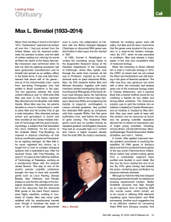


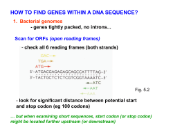

© Copyright 2026