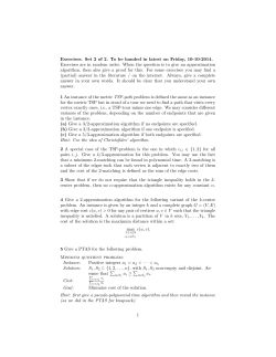
2015
http://excel.fit.vutbr.cz
Evaluation of Schedule Characteristics in RCPSP
ˇ
Petr Sebek*,
Martin Hrub´y**
Abstract
In this paper, I study the resource-constrained project scheduling problem and describe the novel
genetic algorithm GARTH created by Martin Hrub´y. GARTH is designed to find and eliminate
unfavorable characteristics from an individual. This approach is opposing the standard way of
thinking about genetic algorithms – to synthesize desirable characteristic in a new individual. To
be able to recognize unfavorable characteristics, the algorithm creates a hypothesis about mutual
time properties of particular jobs from the given problem instance. This hypothesis is called Run
Time Hypothesis because it is created as the algorithm get to know specific problem instance. The
topic of my paper is to develop this algorithm and to discover new techniques that could be used in
computation of RCPSP.
Keywords: Genetic Algorithm — Resource Constrainded Project Scheduling Problem — GARTH
Supplementary Material: N/A
* [email protected], Faculty of Information Technology, Brno University of Technology
** [email protected], Faculty of Information Technology, Brno University of Technology
1. Introduction
Decisions how to plan a project are done every day
and mistakes or just misjudgments can costs incredible amounts of money. If companies optimize their
projects plans they can achieve a competition advantage and seize control over market. Operational research and its part project scheduling tries to address
these kinds of problems. It tries to come up with better,
more informed decisions.
The problem that this paper is dealing with is to
schedule a project consisting of a number of activities
of known durations and resource demands to resources
of limited capacity. Activities are in precedence relation so we can model what exactly has to be done
before the particular activity can start.
This problem was formulated as the resource-constrained project scheduling problem (RCPSP). RCPSP
of N activities and K resources is a tuple (J, P, R, c, d, r)
where:
• J = { j0 , j1 , . . . , jN , jN+1 } is a set of jobs.
• P ⊆ J × J is an activity precedence relation. Pi
denotes a set of all jobs that must be completed
before job i may start.
• R = {r1 , . . . , rK } is a set of renewable resources.
• c : R → N denotes the capacity of resource.
• d : J → N assigns a non-negative duration to
each job.
• r : J × R → N are resource requirements of job
on resource.
Activity j0 is called start activity, jN+1 is called end
activity. They meet these conditions:
• j0 is the predecessor of all other activities.
• jN+1 is the successor of all other activities.
• d( j0 ) = d( jN+1 ) = 0.
Schedule S is a vector of start times of activities s(S) = (s j ) j∈J . Let vector f denote finish times,
∀ j ∈ J : f j (S) = s j (S) + d( j). We denote schedule
makespan as M(S) = f jN+1 (S) − s j0 (S).
Schedule S is feasible if it meets precedence (1)
and resource (2) constraints:
∀ j ∈ J, ∀i ∈ Pj : s j ≥ si + d(i) (1)
∀k ∈ R,t = 0, . . . , fN+1 :
∑
r( j, k) ≤ c(k) (2)
j∈J,s j ≤t< f j
To optimize RCPSP means to find a feasible schedule with the minimal makespan.
We can optimize the problem with two approaches.
One is trying to find a schedule with the minimal
makespan. This means that we need to explore the
whole state space or use some techniques to reduce it
and prove that no better solution than the found one exists. This is the way of exact algorithms, in my article
I will describe its counterpart – heuristic algorithms.
Heuristic algorithms are designed to come up with
a near-optimal solution in the reasonable amount of
time. I will present some existing heuristics solving
RCPSP related to the algorithm of Martin Hrub´y. For
the overview of the state of the art in the heuristic
RCPSP optimization see [1] or [2].
The simulated annealing (SA) is a probabilistic
metaheuristic [3] for the global optimization. The
origin of this algorithm comes from annealing in metallurgy, which is a technique of controlled heating
and cooling metal to create bigger and better crystals
in material. It is local search algorithm that changes
its current solution if one of its neighbors is better
or worse, but in this case only with some predefined
probability.
The tabu search (TS) is another improving heuristic with local search [4]. The list of few last states (tabu
list) is remembered and avoided when deciding where
to move next. This idea of tabu list should prevent
from cycling in already examined states.
Population-based metaheuristics [5] are algorithms
that have a set of solutions called population and in
each step we create new individuals either from the
population or we generate them out of thin air. Very
promising subarea are genetic algorithms (GA). GA
mimic process of natural selection. Individuals in the
population are considered according to their fitness
function (the makespan in our case). If the individual
is found beneficial to the population, its genes (some
or all values of his representation) will appear also
in upcoming population. There are operations known
from real world used to create a new individual: the
crossover and the mutation.
Genetic Algorithm driven with Run Time Hypothesis [6] (GARTH) belongs to the class of population
based genetic algorithms. It is designed to learn what
characteristics spoil the resulting schedule and then
to eliminate them. GARTH is similar to other genetic
algorithms except for notion of schedule characteristics and Run Time Hypothesis. Run Time Hypothesis
allows us to make informed decisions during mutation
instead of a random choice. In my work I am trying to
develop GARTH and discover its properties.
GARTH is very promising in the field of RCPSP
solvers because it offers a new point of view to the
problem and its results are comparable only with the
best RCPSP solvers.
2. Characteristics Excluding a Solution
The concept of schedule characteristics and especially
their property to exclude a solution is the main contribution of GARTH to the field. It offers an opportunity
to better understand given problem instance.
2.1 Schedule Characteristics
GARTH uses the set of time relations between activities called schedule characteristics to depict a particular schedule. Let ξi j denote a schedule characteristic
of type ξ ∈ {PSE, FLE, SLT, SLF, INT }1 between activities i, j ∈ J \ { j0 , jN+1 }. Abbreviations stands for:
PSE – parallel start, FLE – finish later or equal, SLT
– start later than, SLF – start later than finish, INT –
overlaps.
The schedule characteristics PSEi j and INTi j are
valid in the context of problem instance G, if parallel
run of i and j does not violate their precedence and
resource constraint. The characteristics FLEi j , SLTi j
and SLFi j are valid if j ∈
/ Pi . Let CHG denote a set of
all valid schedule characteristics in G.
Definition 1. Assume schedule S ∈ SG . CHS ⊆ CHG
is a set of S’s characteristics, if for all distinct i, j ∈
J \ { j0 , jN+1 }:
•
•
•
•
•
si (S) = s j (S) ⇔ PSEi j ∈ CHS ,
fi (S) ≤ f j (S) ⇔ FLEi j ∈ CHS ,
si (S) < s j (S) ⇔ SLTi j ∈ CHS .
fi (S) ≤ s j (S) ⇔ SLFi j ∈ CHS
(si (S) ≤ s j (S) ∧ fi (S) > s j (S)) ∨
(s j (S) ≤ si (S) ∧ f j (S) > si (S) ⇔ INTi j ∈ CHS
Regarding a particular problem instance G we need
to distinguish between set of all feasible schedules SG
and set of active schedules SAG so there holds SAG ⊆
SG [7]. Proofs of following theorems can be found
in [6].
For following theorems I need to split schedules
and characteristics according to a makespan.
Definition 2. Decomposition of a set of schedules
according to a makespan:
• [S]m = {S ∈ SG |M(S) = m}
• [SA ]m = {S ∈ SAG |M(S) = m}
1 Characteristics SLF and INT are not included in the original
paper [6]. I defined them because they are used further in the
method Problem Instance Bonding.
we do not find it at a certain makespan level while at
greater makespan we do. This is a complication for
us because schedules we generate belong to SAG . But
whenever a characteristic is excluding a solution with
a makespan m in SG it is certainly excluding a solution
with a makespan m in SAG also.
start ( )
start ( )
start ( )
Resource Utilization
start ( )
Theorem 2. Assume ξi j excluding some makespan m.
Then there is no active schedule S ∈ [SA ]m0 such that
ξi j ∈ CHS for all m0 ≤ m.
0
1
2
3
0
1
Time
2
3
Time
Figure 1. In the left schedule characteristic ” starts
before ” excludes a solution with makespan 2
provided precedence ordering in the top of the image
and displayed resource constraints and activity
durations. On the right you can see that once we
remove this characteristic we get schedule with lower
makespan.
Definition 3. Decomposition of valid characteristics
according to a makespan:
[CHG ]m =
[
CHS
S∈[S]m
Definition 4. Assume a problem instance G and a
particular schedule characteristic ξi j ∈ CHG . Then ξi j
is said to be excluding a solution at a makespan m, if
there is no schedule S ∈ [S]m so that ξi j ∈ CHS .
Reader can find an example of excluding characteristic in Figure 1.
Theorem 1 (Exclusion theorem). Assume a problem
instance G and a particular ξi j so that ξi j ∈ [CHG ]m
and ξi j ∈
/ [CHG ]m−1 for some m. Then:
• ∀m0 ≥ m : ξi j ∈ [CHG ]m0 ,
• ∀m0 < m : ξi j ∈
/ [CHG ]m0 .
This is the most important theorem of the original
paper [6]. It claims that once we find characteristic
that is present in a schedule with makespan m and not
in any schedule with m − 1 we can be sure that this
characteristic will not appear in any schedule with a
makespan < m.
Theorem 1 holds in SG . Unfortunately we cannot
claim this in domain of active schedules SAG . We
cannot ensure that characteristic is excluding when
This knowledge about inner rules of problem instance can help us to optimize more focused to the
optimal solution mopt . If we eliminated all characteristics which are excluding solutions with a makespan
> mopt , we could reach optimal solution quite easily.
But there is a problem: we do not know characteristics
that are excluding solution at certain makespans. We
can only guess which they are according to our previous search. This guess is in terms of GARTH named
Run Time Hypothesis.
2.2 Run Time Hypothesis
To know whether a characteristic excludes a solution at
some makespan we would need to evaluate all possible
schedules and then we could claim that this characteristic is indeed excluding a better solution. Of course this
is not feasible, we would evaluate all possible schedules for knowledge that is meaningless at the moment
we have all schedules (because we already have our
optimal solution).
On the other hand, we can perform many experiments, check their characteristics and if some of them
are not appearing in schedules with better makespan
than some m we can claim that these characteristics
are possibly excluding solutions at makespans < m.
This hypothesis then helps algorithm to make more
informed decisions about what characteristics of the
current schedule to eliminate.
Technically we are holding information about past
characteristics’ makespans in the package of matrices
RTξ of size |J| × |J| called RT system. RTξ (i, j) then
corresponds to the best seen makespan of characteristic
ξi j .
The simplest heuristic based on RT system picks
activities that form characteristic (present in current
schedule S) with the worst value in the RT system
formally:
CHwS = arg max [RTξ (i, j)]
(3)
w
Jch
(S) = {i, j ∈ J|ξi j ∈ CHwS }
(4)
ξi j ∈CHS
w (S) (w as the worst characteristics) are
Activities in Jch
candidates for mutation introduced further.
3. Genetic Algorithm driven with Run
Time Hypothesis (GARTH)
GARTH is an algorithm designed by Martin Hrub´y [6]
who also introduced the concept of schedule characteristics. It is standard genetic algorithm that takes the
best building blocks from other methods invented so
far and together with run time hypothesis draw up an
approach that not only overcomes other algorithms but
also better understands presented problem.
3.1 Solution Encoding
In every genetic algorithm we have to represent our
individual in some way. This representation should
offer an evaluation of fitness function, mutation and
crossover. Prevailing [1] representation is the activity
list. An activity list gives us an order in which we
take activities to create a schedule. In GARTH there
is used standardization of activity lists to assure that
each schedule corresponds with exactly one standardized activity list, in original definition we could have
different activity lists that represent the same schedule.
We cannot represent our individual as a schedule
because work with this structure would be very computationally demanding. But we need a schedule to
evaluate a makespan and to discover time characteristics of a given solution. To convert an activity list to a
schedule we use so-called Schedule Generator Scheme
(SGS), specifically Serial SGS (SSGS) that produces
active schedules (schedules from SAG ). In GARTH we
use Reverse SGS (RSGS) that first uses activity list to
create schedule with SSGS then we take reversed order
of activity ends and creates schedule that is aligned
to the right. This idea that came up from improving
technique known as Justification [8] or Forward Backward Improvement has a noticeable positive impact on
schedule makespan.
During evolution it can happen that some individuals appear in population twice or more. We want to
avoid this situation because equal individuals occupy
places for diverse individual with possibly better attributes. To address this problem we use Population
Normalization, that after every step of genetic algorithm eliminates equal individuals and replaces them
with freshly generated ones. Population Normalization also provides positive source of randomness to the
evolutionary process.
points purely randomly but choose first point c1 from
range 1, . . . , 2N
5 . Second point c2 is set to c2 = c1 + ∆
3N
where ∆ is a random number from range 2N
5 ,..., 5 .
The small mutation comes optionally after the
crossover. Three randomly selected jobs from the
child’s activity list are shifted in a random order up to
where precedence constraints allow.
In the mutation we use knowledge from our RT
system to make informed decision what activities to
w (equation 4) up to
shift. We choose activities from Jch
some predefined number. We shift with each activity in
random direction. These activities represent excluding
characteristics of the schedule. From this operation we
expect to break excluding characteristics and reach a
schedule with a better makespan.
3.3 GARTH Algorithm
In the previous sections I presented all building blocks
of GARTH algorithm. For the complete algorithm
please see [6]. GARTH is mostly a standard genetic
algorithm. It has population of individuals that is each
step evaluated and that generates new population. It
uses elitism concept, i.e. the number of best individuals are chosen to be unchanged in the new population.
Some of randomly chosen individuals are mutated using Run Time Hypothesis. The rest of individuals is
generated by the crossover optionally followed by the
small mutation. First parent for the crossover comes
from the new population and second comes from the
old population. This selection of parents helps best and
mutated individuals to influence new population right
in the evolutionary cycle. After the new population is
full it is evaluated, normalized and the cycle begins
again.
3.4 Evaluation on the Fly
I designed and tested one simple improvement of GARTH
called Evaluation on the fly (EOTF). In standard GARTH
we perform mutation and crossover operation and then
evaluate this new population as a whole. You can notice that the activity list of the first parent that enters to
crossover is not normalized at the time. Either it was
mutated or recombined. Evaluation on the fly fixes
this flaw. It evaluates each individual at the moment
it is generated so the crossover can operate always on
normalized activity lists.
Another improving effect is that EOTF allows not
to evaluate best individuals which were already evalu3.2 Genetic Operations
ated in the last iteration and thus save some schedules
In GARTH we use three genetic operations: the crossover, from schedule generation limit. But applying this printhe small mutation and the mutation. The crossover is ciple too aggressively would forbid best schedules to
the standard two-point crossover [9] with the modifi- perform justification. Therefore, we control if schedcation introduced in [10]. We do not choose crossing ule’s makespan was improved due to previous gener-
ation and if not we do not evaluate it again to get the
same result. You can see experimental results of EOTF
in the Section 4.
3.5 Problem Instance Bonding
Another potential improvement that is my contribution
to the GARTH is the Problem Instance Bonding (PIB).
In the regular GARTH algorithm we try to eliminate
characteristics excluding better solution by mutation.
This mutation does not guarantee that said characteristic in a schedule will be eliminated.
The way how to forbid a characteristic for sure is
to add a precedence constraint between its activities.
This is the way how the PIB works. It lets the RT system with SLF and INT characteristics to gain needed
knowledge about a problem instance, then it picks several suitable characteristics with high makespan and to
an original problem adds edges opposite to characteristics. More formally PIB chooses characteristic SLFi j
if:
RTSLF (i, j) > threshold ∧
RTSLF ( j, i) ≤ threshold ∧
RTINT (i, j) ≥ RTSLF (i, j)
where threshold is experimentally set to the makespan
of the best schedule plus 10. In other words PIB
searches for activities that have poor results in one
ordering and also while running in parallel, and not in
reverse ordering. This gives us a place for a new edge
( j, i). Edge is added in a way that it does not create a
cycle in a precedence graph.
The hypothesis behind the PIB is that by restricting
a state space of a problem instance we should be able
to reach the optimal solution faster. This method can
be potentially dangerous because by adding constraints
we can eliminate optimal schedules from a state space.
4. Experimental Results
To move GARTH further I need to state hypotheses and
then evaluate them. Thus the most important part of my
work are experiments. Fortunately RCPSP has standardized set of problem instances called PSPLIB [11]
that is accepted as main evaluation criteria of all algorithms in the field. I conducted my experiments on
sets of 60 and 120 activities (denoted as J60 and J120).
The set of 30 activities is completely computed for a
long time and has small informative value. All experiments are intended to perform with limit of generated
schedules as comparative criterion. Usually it is 5,000
and 50,000 schedules per test. Again I will perform
only experiments with higher number of generated
schedules because in 5,000 schedules limit algorithm
does not have time to employ its strength – RT System. Results are evaluated as average of deviation
from critical path lower bound [2] for each instance,
while each instance was run 10 times to reduce effect
of chance. The best results on PSPLIB are 10.63 for
J60 and 30.66 for J120 [10]. In my experiments I am
not trying to compete with the best results but to show
benefit of used techniques relatively.
My first task is to confirm that GARTH actually
works and results stated in [6] are correct. As my
implementation of GARTH is still a prototype and
needs to be tuned more I did not reach result from
the original paper, but I can confirm positive impact
of RT Characteristics on given problems. As you can
see in the Table 1 RT system really takes its place in
computation. BRTSA is a simple iterative algorithm
that mutates all individuals according to characteristic
in RTS (if RTS = 0/ it mutates random activities) and
keeps record of the best individuals. GARTH-3 is an
GARTH variant where no individual is mutated and all
are recombined and GARTH-7 is full GARTH with delayed RT startup. Even the simplest algorithm BRTSA
can claim that RT system helps its results, there is an
evident improvement in results when RT characteristic
is employed. GARTH-3 serves as indicator how far we
can get with simple algorithm without RT characteristic. Results of GARTH-7 definitely show contribution
of RT characteristic as they are comparable to other
algorithms published in [1].
Table 1. Overview of results
Algorithm RTS
BRTSA
BRTSA
GARTH-3
GARTH-7
0/
SLT
0/
PSE, FLE, SLT
J60 J120
11.16
11.00
10.82
10.76
33.44
33.00
32.20
31.59
My first attempt to improve results of GARTH
was based on hypothesis that if some problem instance
response better to a particular characteristic or a combination of them then we could create a procedure that
decides what characteristic to use to achieve better
results. However, majority of results over characteristics from power set 2{PSE,FLE,SLT } was the same or
very similar so no meaningful division of problem instance and therefore no suitable decision tree could be
created.
Next experiment takes as a goal to assess benefit
of using Evaluation on the fly (EOTF), which was
described in Section 3.3. You can see the results of
GARTH-7 with and without EOTF in the Table 2. The
improvement is small but consistent as the change does
not influence algorithm much. The Evaluation on the
fly certainly can improve the original algorithm.
Table 2. Evaluation on the fly
Set
Characteristic GARTH-7 EOTF
J60
PSE
FLE
SLT
10.766 10.758
10.775 10.738
10.769 10.759
PSE
J120 FLE
SLT
31.695 31.583
31.667 31.507
31.665 31.587
Third evaluated experiment deals with Problem
Instance Bonding. I ran experiment with various parameter settings (how often to add how many new
edges) but unfortunately this approach to reduce the
state space of a problem instance did not go well. The
best result I have achieved with GARTH-7 on J60 set
was 10.78 (which is worse than without PIB) with
adding 10 new edges every 10 iterations of the algorithm. I noticed that after adding new edges the best
solutions was lost because some of the activity lists
was not feasible in the new problem settings and other
had to be recalculated.
5. Conclusions
In this paper I described and formalized the resourceconstrained project scheduling problem. I presented
novel algorithm called Genetic Algorithm driven with
Run Time Hypothesis that introduces concept of schedule characteristics and their use to better optimization
in RCPSP. I designed few improvements and evaluated them on standardized set of problem instances
PSPLIB.
I partly confirmed experimental results of original
paper about GARTH, mainly the benefit of using RT
system. I also designed the new improvement Evaluation on the fly that stably improves all results by about
0.1 and more. My another contribution was the idea
of Problem Instance Bonding method using notion of
characteristics excluding a better solution in restricting state space of the given problem. This approach
require more research.
GARTH is indeed really promising algorithm to
solve RCPSP. There are still places to improve this
method, whether it is other kinds of schedule characteristics or their better utilization. I would like to
research adapting parameters and higher order Run
Time Hypothesis.
References
[1] Rainer Kolisch and S¨onke Hartmann. Experimental investigation of heuristics for resourceconstrained project scheduling: An update.
European Journal of Operational Research,
174(1):23–37, 2006.
[2] Christian Artigues, Sophie Demassey, and Emmanuel Neron. Resource-constrained project
scheduling: models, algorithms, extensions and
applications, volume 37. John Wiley & Sons,
2010.
[3] Scott Kirkpatrick, MP Vecchi, et al. Optimization by simmulated annealing. science,
220(4598):671–680, 1983.
[4] Fred Glover. Tabu search-part i. ORSA Journal
on computing, 1(3):190–206, 1989.
[5] Christian Blum and Andrea Roli. Metaheuristics in combinatorial optimization: Overview and
conceptual comparison. ACM Computing Surveys (CSUR), 35(3):268–308, 2003.
[6] Martin Hrub´y. A dynamic analysis of resourceconstrained project scheduling problems for an
informed search via genetic algorithm optimization. European Journal of Operational Research,
2015. In review.
[7] Arno Sprecher, Rainer Kolisch, and Andreas
Drexl. Semi-active, active, and non-delay schedules for the resource-constrained project scheduling problem. European Journal of Operational
Research, 80(1):94–102, 1995.
[8] Vicente Valls, Francisco Ballest´ın, and Sacramento Quintanilla. Justification and rcpsp: A
technique that pays. European Journal of Operational Research, 165(2):375–386, 2005.
[9] S¨onke Hartmann. A competitive genetic algorithm for resource-constrained project scheduling. Naval Research Logistics (NRL), 45(7):733–
750, 1998.
[10] Andrew Lim, Hong Ma, Brian Rodrigues,
Sun Teck Tan, and Fei Xiao. New meta-heuristics
for the resource-constrained project scheduling
problem. Flexible Services and Manufacturing
Journal, 25(1-2):48–73, 2013.
[11] Rainer Kolisch and Arno Sprecher. Psplib-a
project scheduling problem library: Or softwareorsep operations research software exchange program. European Journal of Operational Research, 96(1):205–216, 1997.