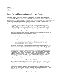
Architectures and precision analysis for modelling
atmospheric variables with chaotic behaviour
FCCM 2015
Peter D. D¨
uben‡
Francis P. Russell†
Xinyu Niu† Wayne Luk†
Tim N. Palmer‡
Imperial College London† & Oxford University‡
05/05/2015
Francis P. Russell
Chaotic Systems in Hardware
05/05/2015
1 / 16
Weather Modelling
Atmospheric modelling requires simulation of a chaotic system.
Chaotic systems are highly sensitive to initial conditions - the
butterfly effect.
There are many sources of uncertainly in atmospheric simulations.
Sets of multiple simulations, called emsembles are run to build a
distribution of outcomes.
Lorenz’96 is a simple model designed by Lorenz to study predictability
in chaotic systems.
We study the two-scale Lorenz’96 system which models small and
large-scale dynamics.
Francis P. Russell
Chaotic Systems in Hardware
05/05/2015
2 / 16
The Lorenz’96 system (K=6, J=8)
local-scale values
Y4,6
Y5,6
Y6,6
Y7,6
Y8,6
Y1,1
Y3,6
Y2,1
Y2,6
Y3,1
Y1,6
Y4,1
Y8,5
Y5,1
Y7,5
Y6,1
X6
Y6,5
Y7,1
X1
Y5,5
Y8,1
Y4,5
Y1,2
X5
Y3,5
Y2,2
global-scale values
Y2,5
Y3,2
X2
Y1,5
Y4,2
Y8,4
Y5,2
X4
Y7,4
Y6,2
X3
Y6,4
Y7,2
Y5,4
dXk
= − Xk−1 (Xk−2 − Xk+1 )
dt
J
hc X
− Xk + F −
Yj,k
b
j=1
dYj,k
= − cbYj+1,k (Yj+2,k
dt
− Yj−1,k )
hc
− cYj,k +
Xk
b
Y8,2
Y4,4
Y1,3
Y3,4
Y2,3
Y2,4
Y3,3
Y1,4
Y8,3
Francis P. Russell
Y7,3
Y6,3
Y5,3
Y4,3
Typically, the largest J of interest
≈ 128. We increase the value of K
when increasing system size (up to
≈ 800,000).
Chaotic Systems in Hardware
05/05/2015
3 / 16
Contributions
A hardware design of the two-scale Lorenz’96 system, useful for
studying the effects of multi-scale interactions in weather modelling.
Demonstration of how trade-offs can be made between precision and
throughput for the hardware implementation of a system with chaotic
behaviour.
Present an analysis of the precision reduction impact on a hardware
implementation of Lorenz’96 using metrics appropriate for chaotic
systems.
Show the effects on power and performance, and compare to an
optimised CPU implementation.
Francis P. Russell
Chaotic Systems in Hardware
05/05/2015
4 / 16
Hardware Design
Off-chip
Memory
Pipelined Runge-Kutta
timestepping.
Different precisions for global
and local-scale quantities.
Strip
Padding
Deinterleave
R-K
Step 1
R-K
Step 2
Local-scale values processed
with customisable vector width.
Periodic boundary conditions
are problematic for a streaming
design.
Periodic properties of the
system are used to enable
in-place updates, “rotating”
the system each update.
Francis P. Russell
R-K
Step 4
R-K
Step 3
Off-chip
Memory
Chaotic Systems in Hardware
Pad
Interleave
05/05/2015
5 / 16
How much precision is enough?
Computational scientists typically only have to choose between single
and double precision.
Choosing double precision is the simplest way to avoid thinking about
the way individual degrees of freedom have been discretised.
We can usually compare a reduction precision implementation against
an analytical solution for simple test cases and a high-precision
implementation for more complex ones.
Neither of these approaches is directly applicable to chaotic systems due to
the Butterfly effect.
Francis P. Russell
Chaotic Systems in Hardware
05/05/2015
6 / 16
Error metrics
We cannot compare long runs of Lorenz’96 at different precisions
using standard error metrics.
Even when starting from the same initial conditions, we expect the
chaotic nature to magnify effects of different number representations,
order of operations and other implementation artefacts.
We use the Hellinger distance to compare the probability density
functions of the global and local-scale values of the simulation.
For two probability density functions p and q, the Hellinger distance is
defined as:
s Z
2
p
1 p
H(p, q) =
p(x) − q(x) dx
2
Francis P. Russell
Chaotic Systems in Hardware
05/05/2015
7 / 16
Estimating the error
Using an arbitrary precision CPU-implementation we vary the precision of
local and global-scale associated values. Distances are compared against
those of a double-precision implementation.
20
15
10
5
5
10
15
20
global-scale mantissa (bits)
0.945
0.840
0.735
0.630
0.525
0.420
0.315
0.210
0.105
0.000
Local-scale (Y) distances
local-scale mantissa (bits)
local-scale mantissa (bits)
Global-scale (X) distances
0.54
0.48
0.42
0.36
0.30
0.24
0.18
0.12
0.06
0.00
20
15
10
5
5
10
15
20
global-scale mantissa (bits)
Precision changes in variables at one scale do not typically affect those at
the other, so we could optimise them independently.
Francis P. Russell
Chaotic Systems in Hardware
05/05/2015
8 / 16
Estimating appropriate mantissa sizes
Using the CPU-based reduced-precision analysis, we can calculate
minimum mantissa widths for local and global-scale values, depending on
the amount of error we are willing to accept.
Run
Changed initial conditions
c × 0.99, F × 0.99
c × 1.01, F × 1.01
c × 0.9, F × 0.9
c × 1.1, F × 1.1
H
(global)
H
(local)
2.788e-3
4.605e-3
5.042e-3
4.047e-2
3.620e-2
1.939e-4
1.505e-3
1.719e-3
1.625e-2
1.415e-2
Est.
min.
mantissa
(global)
15
13
13
11
11
Est.
min.
mantissa
(local)
12
10
10
9
9
Scaling c and F represents variation in the input parameters by 1 and 10%
due to measurement uncertainty.
Francis P. Russell
Chaotic Systems in Hardware
05/05/2015
9 / 16
Profiling exponent ranges
We also use the CPU-based implementation to profile exponent ranges for
the global and local-scale values.
local-scale
frequency (normalised)
frequency (normalised)
global-scale
0.25
0.2
0.15
0.1
0.05
0
-15
-10
-5
0
5
base-2 exponent
10
0.2
0.18
0.16
0.14
0.12
0.1
0.08
0.06
0.04
0.02
0
-15
-10
-5
0
5
base-2 exponent
10
Most exponents are ≤ 9 so we need at least 5 bits for both global and
local-scale (signed) exponent values.
Francis P. Russell
Chaotic Systems in Hardware
05/05/2015
10 / 16
The resulting designs
We build designs1 at different precisions, allowing us to process different
number of input elements per cycle (the vector width).
DFE1 Uses single precision.
DFE2 Estimated precision for minimal effect on result.
DFE32 /4 Estimated as similar error to 1% variation in input
parameters.
Build
DFE1
DFE2
DFE3
DFE4
1
2
Global-scale
type
float(8, 24)
float(6, 15)
float(5, 13)
float(5, 13)
Local-scale
type
float(8, 24)
float(5, 12)
float(5, 10)
float(5, 10)
Vector
width
8
16
16
24
Utilisation
Logic DSP
55.00 48.16
69.85 32.84
64.28 32.84
79.15 47.92
(%)
BRAM
24.25
28.67
27.63
33.74
Maxeler MAX3A Vectis Dataflow Engine (Xilinx Virtex6 SXT475).
Used to facilitate accuracy comparisons with the CPU-based implementation.
Francis P. Russell
Chaotic Systems in Hardware
05/05/2015
11 / 16
Precision Results
For J = 64 (which the CPU-simulations were run with) we have similar
errors to those predicted by the CPU-simulations. For J = 144, we have
slightly larger errors, but still acceptable for use.
Build
Changed initial cond.
c × 0.99, F × 0.99
c × 1.01, F × 1.01
c × 0.9, F × 0.9
c × 1.1, F × 1.1
DFE1 (g=f(8,24), l=f(8,24), w=8)
DFE2 (g=f(6,15), l=f(5,12), w=16)
DFE3 (g=f(5,13), l=f(5,10), w=16)
DFE4 (g=f(5,13), l=f(5,10), w=24)
Francis P. Russell
J = 64
H
H
(global)
(local)
2.788e-3
1.939e-4
4.605e-3
1.505e-3
5.042e-3
1.719e-3
4.047e-2
1.625e-2
3.620e-2
1.415e-2
2.934e-3
2.881e-4
2.776e-3
2.707e-4
3.267e-3
6.742e-4
N/A
N/A
Chaotic Systems in Hardware
J = 144
H
H
(global)
(local)
7.029e-3
6.291e-4
1.399e-2
1.726e-3
1.067e-2
1.861e-3
1.167e-1
1.487e-2
8.826e-2
1.236e-2
7.472e-3
1.180e-3
4.320e-2
2.443e-3
7.289e-2
1.012e-2
7.404e-2
1.005e-2
05/05/2015
12 / 16
Precision Results
For J = 64 (which the CPU-simulations were run with) we have similar
errors to those predicted by the CPU-simulations. For J = 144, we have
slightly larger errors, but still acceptable for use.
Build
Changed initial cond.
c × 0.99, F × 0.99
c × 1.01, F × 1.01
c × 0.9, F × 0.9
c × 1.1, F × 1.1
DFE1 (g=f(8,24), l=f(8,24), w=8)
DFE2 (g=f(6,15), l=f(5,12), w=16)
DFE3 (g=f(5,13), l=f(5,10), w=16)
DFE4 (g=f(5,13), l=f(5,10), w=24)
Francis P. Russell
J = 64
H
H
(global)
(local)
2.788e-3
1.939e-4
4.605e-3
1.505e-3
5.042e-3
1.719e-3
4.047e-2
1.625e-2
3.620e-2
1.415e-2
2.934e-3
2.881e-4
2.776e-3
2.707e-4
3.267e-3
6.742e-4
N/A
N/A
Chaotic Systems in Hardware
J = 144
H
H
(global)
(local)
7.029e-3
6.291e-4
1.399e-2
1.726e-3
1.067e-2
1.861e-3
1.167e-1
1.487e-2
8.826e-2
1.236e-2
7.472e-3
1.180e-3
4.320e-2
2.443e-3
7.289e-2
1.012e-2
7.404e-2
1.005e-2
05/05/2015
12 / 16
Precision Results
For J = 64 (which the CPU-simulations were run with) we have similar
errors to those predicted by the CPU-simulations. For J = 144, we have
slightly larger errors, but still acceptable for use.
Build
Changed initial cond.
c × 0.99, F × 0.99
c × 1.01, F × 1.01
c × 0.9, F × 0.9
c × 1.1, F × 1.1
DFE1 (g=f(8,24), l=f(8,24), w=8)
DFE2 (g=f(6,15), l=f(5,12), w=16)
DFE3 (g=f(5,13), l=f(5,10), w=16)
DFE4 (g=f(5,13), l=f(5,10), w=24)
Francis P. Russell
J = 64
H
H
(global)
(local)
2.788e-3
1.939e-4
4.605e-3
1.505e-3
5.042e-3
1.719e-3
4.047e-2
1.625e-2
3.620e-2
1.415e-2
2.934e-3
2.881e-4
2.776e-3
2.707e-4
3.267e-3
6.742e-4
N/A
N/A
Chaotic Systems in Hardware
J = 144
H
H
(global)
(local)
7.029e-3
6.291e-4
1.399e-2
1.726e-3
1.067e-2
1.861e-3
1.167e-1
1.487e-2
8.826e-2
1.236e-2
7.472e-3
1.180e-3
4.320e-2
2.443e-3
7.289e-2
1.012e-2
7.404e-2
1.005e-2
05/05/2015
12 / 16
Precision Results
For J = 64 (which the CPU-simulations were run with) we have similar
errors to those predicted by the CPU-simulations. For J = 144, we have
slightly larger errors, but still acceptable for use.
Build
Changed initial cond.
c × 0.99, F × 0.99
c × 1.01, F × 1.01
c × 0.9, F × 0.9
c × 1.1, F × 1.1
DFE1 (g=f(8,24), l=f(8,24), w=8)
DFE2 (g=f(6,15), l=f(5,12), w=16)
DFE3 (g=f(5,13), l=f(5,10), w=16)
DFE4 (g=f(5,13), l=f(5,10), w=24)
Francis P. Russell
J = 64
H
H
(global)
(local)
2.788e-3
1.939e-4
4.605e-3
1.505e-3
5.042e-3
1.719e-3
4.047e-2
1.625e-2
3.620e-2
1.415e-2
2.934e-3
2.881e-4
2.776e-3
2.707e-4
3.267e-3
6.742e-4
N/A
N/A
Chaotic Systems in Hardware
J = 144
H
H
(global)
(local)
7.029e-3
6.291e-4
1.399e-2
1.726e-3
1.067e-2
1.861e-3
1.167e-1
1.487e-2
8.826e-2
1.236e-2
7.472e-3
1.180e-3
4.320e-2
2.443e-3
7.289e-2
1.012e-2
7.404e-2
1.005e-2
05/05/2015
12 / 16
Performance (J=144, float system size: 227KiB - 453MiB)
4.5e+09
FPGA1 (g=f(5,13), l=f(5,10), w=24) (DFE4)
FPGA1 (g=f(6,15), l=f(5,12), w=16) (DFE2)
FPGA1 (g=f(8,24), l=f(8,24), w=8) (DFE1)
CPU2 (single-precision, 12 cores)
CPU2 (double-precision, 12 cores)
4e+09
elements/second
3.5e+09
3e+09
6.93×
2.5e+09
2e+09
5.37×
1.5e+09
1e+09
2.83×
5e+08
0
100
1
2
0.514×
1000
10000
K (log-scale)
100000
1e+06
Maxeler MAX3A Vectis DFE (Xilinx Virtex6 SXT475 @ 150MHz).
Dual-socket hyperthreaded Intel Xeon X5660s @ 2.67GHz.
Francis P. Russell
Chaotic Systems in Hardware
05/05/2015
13 / 16
Power Efficiency
We measure the power requirements of a software implementation on two
different systems and compare against the most power efficient.
Build Throughput
(elements/s)
System 12 (4-cores) 1.63e8
System 23 (6-cores) 2.05e8
System 2 (12-cores) 4.05e8
DFE1 (System 1) 1.14e9
DFE2 (System 1) 2.17e9
DFE4 (System 1) 2.81e9
Power (W)
2081
3991
5031
137
143
146
Efficiency
Relative
(elements/J) Efficiency
7.83e5
0.972
5.14e5
0.638
8.05e5
1.00
8.35e6
10.4
1.52e7
18.9
1.92e7
23.9
1
Power consumption of unused Maxeler cards subtracted.
Hyperthreaded Intel Core i7 870 @ 2.93GHz
3
Dual-socket hyperthreaded Intel Xeon X5660s @ 2.67GHz.
2
Francis P. Russell
Chaotic Systems in Hardware
05/05/2015
14 / 16
Future work
More complex models like shallow water.
More sophisticated means for incorporating input-value uncertainty
into a simulation.
Generate designs from a domain-specific languages, allowing domain
specialists to supply uncertainty information directly.
Francis P. Russell
Chaotic Systems in Hardware
05/05/2015
15 / 16
Conclusions
Obtaining near-identical numerical behaviour to a reference solution is
not always the best goal.
Chaotic systems force us to re-evaluate how we measure the
correctness of a simulation.
Chaos-aware precision reduction enables us to exploit input-parameter
uncertainty and nature of the chaotic behaviour itself.
We demonstrated how to achieve this for simple chaotic system and
the performance and power benefits over a conventional CPU
implementation.
Weather modelling is a problem that drives the purchase of
supercomputers. Only reconfigurable computing enables us to exploit
the properties of chaotic systems to reduce power and improve
performance.
Francis P. Russell
Chaotic Systems in Hardware
05/05/2015
16 / 16