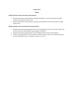
AGC 4
1.0 Problem 11.2
For the isolated generating station with local
load shown in Fig. 1 below, it is observed that
ΔPL=0.1pu brings about Δω=-0.2rad/sec in the
steady-state.
1
R
ΔPL
-
ΔPC +

-

1
s 1
+
10
1  10s
Δω
Fig. 1
(a) Find 1/R.
Solution:
We need the transfer function between Δω and
ΔPL. To get this, write down Δω as a function of
what is coming into it:
ˆ 

10  1  ˆ
1

ˆ
ˆ

P






P

 C

L
1  10s  s  1 
R


1
Now solve for Δω. Expanding:
ˆ 
10  1  ˆ 1

ˆ
ˆ

P





P




C
L
1  10s  s  1 
R


 PˆC
10  1 
10  1  1
10PˆL




 ˆ  
1  10s  s  1  1  10s  s  1  R
 1  10s
Bringing terms in Δω to the left-hand-side:
10  1  1
10  1  10PˆL
ˆ
ˆ 

 ˆ  PC


1  10s  s  1  R
1  10s  s  1  1  10s
Factoring Δω:

10  1  1 
10  1  10PˆL
ˆ
ˆ 1 

   PC


1

10
s
s

1
R
1

10
s
s

1

 

 1  10s

Dividing:
ˆ
10
1
10

P


L
PˆC


1  10s  s  1  1  10s
ˆ 
10  1  1
1


1  10s  s  1  R
Multiply through by (1+10s)(s+1):
10PˆC  10PˆL ( s  1)
ˆ 
10
(1  10s)( s  1) 
R
Rearrange the top and expand the bottom:
2
10PˆC  10( s  1)PˆL
ˆ 
10s 2  11s  (1  10 / R)
(*)
Now we consider ΔPC=0pu, ΔPL=0.1pu, and
assume it is a step change. Therefore:
PˆL 
PL
s
Substituting into (*), we get:
ˆ 
 10( s  1)
PL
10s 2  11s  (1  10 / R) s
The above expression is a LaPlace function (i.e.,
in s). The problem gives data for the steadystate (in time). We may apply the final-value
theorem to the above expression to obtain:
  lim  (t )
t 
 10( s  1)
PL
s 0
s  0 10 s 2  11s  (1  10 / R ) s
 10( s  1)PL
 10PL
 lim

s  0 10 s 2  11s  (1  10 / R )
1  10 / R
 lim sˆ  lim s
that is,
 
 10PL
1  10 / R
3
Solving for R, we obtain:
 10PL
 10PL  
1 


 10
R
10PL  
10 / R 
Substituting ΔPL=0.1pu and Δω=-0.2rad/sec, we
obtain:
R
 10
 10(0.2)

 2.5
10PL   10(0.1)  (0.2)
The problem was specified with power in perunit and Δω in rad/sec. Reference to the block
diagram indicates that the left-hand-side
summing junction outputs ΔPC-Δω/R. To make
this sum have commensurate units, it must be
the case that R has units of (rad/sec)/pu power.
So R=2.5 (rad/sec)/pu power.
The problem asks for 1/R, which would be
1/2.5=0.4 pu power/(rad/sec).
4
One might also express R and 1/R in units of pu
frequency/pu power. This would be:
Rpu=2.5/60=0.0417
1/Rpu=24
Recalling the NERC specification that all units
should have R=0.05, then this R should be
adjusted upwards.
Question: What does an R=0.0417 mean relative
to an R=0.05?
Answer: Recalling that Rpu=-Δωpu/ΔPm,pu, we
can say that Rpu expresses the steady-state
frequency deviation, as a percentage of 60 Hz,
for which the machine will move by an amount
equal to its full rating. So:
 if Rpu=0.05, then the steady-state frequency
deviation for which the machine will move by
an amount equal to its full rating is
0.05*60=3hz.
 if Rpu=0.0417, then the steady-state frequency
deviation for which the machine will move by
an amount equal to its full rating is
0.0417*60=2.502hz.
5
(b) Specify ΔPC to bring Δω back to zero (i.e.,
back to the steady-state frequency ω=ω0).
Solution:
Recalling eq. (*):
10PˆC  10( s  1)PˆL
ˆ 
10s 2  11s  (1  10 / R)
(*)
Now we have that
PˆC 
PC
s
and ΔPL=0. In this case, eq. (*) becomes:
ˆ 
10PC / s
10s 2  11s  (1  10 / R)
Applying the final value theorem again:
  lim  (t )
t 
 lim sˆ  lim s
s 0
s 0
  lim  (t )
t 
10PC / s
s 0
s  0 10 s 2  11s  (1  10 / R )
10PC
10PC
 lim

s  0 10 s 2  11s  (1  10 / R )
1  10 / R
 lim sˆ  lim s
6
that is,
10PC
 
1  10 / R
Solving for ΔPC, we get:
 (1  10 / R)
PC 
10
Having already computed 1/R=0.4 in part (a),
and with Δω=-0.2, we have
PC 
 0.2(1  10 / 2.5)
 0.1
10
which indicates that for this load increase of 0.1
which results (from primary speed control) in a
frequency deviation of -0.2 rad/sec, we need to
adjust the speed-changer motor to increase plant
output by 0.1 pu in order to correct the steadystate frequency deviation back to 0.
The change to the speed-changer motor would
be accomplished by the supplementary control.
7
2.0 Last comments on AGC
Someone asked me about applying the root
locus method as in Example 11.3 of text. Root
locus is a procedure for analysis of stability, that
you would not have learned unless you took EE
475, and so I choose not to cover this.
Hint on Problem 11.3: At the bottom of page
390, the text says: “The reader is invited to
~
~
T
K


M
1
/
/
D
D
check that with Pi
Pi
i
i and
i , Figure
11.10 represents (11.22) in block diagram form.
In Figure 11.10 we have Δωi as an output and
ΔPMi as an input and can close the power control
loop by introducing the turbine-governor block
diagram shown in Figure 11.4.”
This will result in the following block diagram.
1
R
Δω
ΔPL
ΔPC
+
-

1
(1  sTG )(1  sTT )
Δδ
-
ΔPM

+
8
KP
1  sTP
1
s