1
Predicting True Patterns of Cognitive Performance
from Noisy Data
W. Todd Maddox
W. K. Estes
University of Texas, Austin
Indiana University
In press at Psychonomic Bulletin and Review
Abstract
Starting from the premise that the purpose of cognitive modeling is to gain
information about cognitive processes of individuals, we develop a general theoretical
framework for assessment of models on the basis of tests of the models' ability to yield
information about true performance patterns of individual subjects and the processes
underlying them. To address the central problem that observed performance is a
composite of true performance and error, we present formal derivations concerning
inference from noisy data to true performance. Analyses of model fits to simulated data
illustrate the usefulness of our approach for coping with difficult issues of model
identifiability and testablity.
Introduction
In nearly all cognitive research, analyses of data are conducted by
application of statistical methods deriving from the family of linear statistical
models (analysis of variance and covariance, multivariate analysis). The methods
all depend on the assumption that any performance score constitutes a mixture
of two components: One represents true effects of experimental variables
(henceforth, the "true score") and one represents experimental error. Our
premise in this article is that the same assumption holds when scientific models
are applied to the same data. The importance of the assumption stems from our
view that the purpose of cognitive modeling is not simply to describe data but to
gain information about the cognitive processes of individuals that underlie
performance.
In the following sections, we first formalize the problem of inferring true
performance patterns from fits of models to composite data, and derive some
general relationships among observed performance scores, true scores, and
predicted scores generated by model fits. Second, using simulated data for which
the true scores and error components are known, we address the problem of
2
assessing a model's capability for recovering true parameter values from model
fits and generating useful inferences about patterns of true performance.
A Framework for Model-Based Inference of True Performance
Basic Terms and Functions
The presentation and illustration of the methods we propose refer to any
experiment to which we might apply a cognitive model in order to aid inferences about
the output of the experimental subjects' cognitive processes.
The theoretical framework for our methodology follows Estes (2002). Four
aspects of cognitive performance are distinguished: observed performance,
performance predicted by a model, true performance, and error. We denote these by P,
Pr, T, and e, respectively. Each term refers to the performance of an individual subject
on a single experimental trial.
The term T represents the output of the individual's cognitive processes before
the output enters into generation of an observed response, P. The true response, T, is
assumed to have the form of some function of a set (or vector) of parameters, θ, that is,
T = f(θ).
(1)
The function may be explicitly defined, or it may be implicit in a computer program that
generates predictions of performance in the situation. Observed performance is
represented by
P = T + e.
(2)
The error term e is assumed to be normally distributed with a mean of zero and a
standard deviation σ that is unknown a priori but can be estimated from data. Our
specific assumption about the form of the error term is not the only possibility, but it has
the advantage of conforming to long-term usage in statistics and psychometrics.
An alternative expression for observed performance is
P = f(θ). + e,
(3)
obtained by substitution from Equation 1.
For models considered in this article, values of the parameters are not known a
priori, but upon application of the model to an experiment, the parameter values are
estimated from performance data. The estimated parameter vector is denoted θe, and
Pr, performance predicted by the model, is given by
Pr = f(θe),
(4)
where f(θe) is the right hand side of Equation 1 with θ replaced by its estimate.
With this conceptual machinery in hand, we are prepared to approach the
question of how outputs of model fits can yield information about properties of true
3
performance both at a quite general level and also as it arises in analyses of specific
models and experiments.
Derivation of General Relationships between Predicted and True Performance
To illustrate our approach at the more general level, we pose the question of
whether and how constant error, or bias, may arise if the disparities between observed
and predicted performance in the output of a model fit are used to infer corresponding
disparities between predicted and true performance.
We consider first the performance of a subject in a single episode under some
condition of an experiment, using the notation defined above but adding a subscript j (j =
1, 2, ... J) to P and the other terms in order to identify the condition referred to among a
set of J possibilities. Assuming that a model has been fitted to the subject's data, we
seek a relation between Pj - Prj and Tj - Prj. By appropriate application of Equations
1-4, we obtain the identity
Pj - Prj = Tj - Prj + ej.
(5)
For any single episode, the observed difference, Pj - Prj, predicts too high or too low a
value for the true difference, Tj - Prj, depending on the sign of ej. If the episode could
be replicated a large number of times with no change in values of the model's
parameters, mean error would tend to zero and Pj - Prj would be a perfect predictor of
Tj - Prj.
In cognitive research, unlimited replication with constant parameters may not be
possible, but cumulation of Pj - Prj over the conditions of an experiment can inform us
about the corresponding cumulation for Tj - Prj. Assuming that ej is sampled from the
same normal distribution on all trials and averaging the two sides of Equation 5 over
conditions, we obtain
(1/J)Σ( Pj - Prj) = (1/J)Σ(Tj - Prj + ej),
or
M(P - Pr) = M(T - Pr) + M(e).
(6)
If the means are computed for successively larger numbers of conditions (J = 1, 2, ...),
the sign of M(e) may fluctuate, but beyond some J, Jc, it becomes highly unlikely that
further fluctuations will be observed and nearly always the observed difference for J >
Jc, will consistently imply too large or too small a value for the true difference1. The
magnitude of this disparity will progressively decrease, of course, becoming vanishingly
small for sufficently large J.
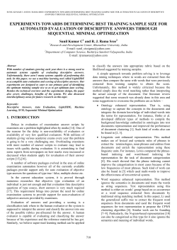
{Figure 1 about here}
For a concrete illustration, Figure 1 presents plots of Equation 6 for
simulated data (curves of forgetting) of two hypothetical subjects whose true
performance is described by the power function Tn = n-.3, with n, corresponding
to j in the preceding derivation, denoting number of unit time intervals.
4
Performance scores were obtained by adding to Tn values of e sampled from
error distributions with σ equal to .02 or .04. Although an n of 100 is not enough
for the functions to reach asymptote, stable relationships between Pj - Prj and Tj
- Prj appear to have emerged by a sequence length of about 60 for the lower
noise and 80 for the higher noise subject.
To treat mean squared disparities, a derivation analogous to that of Equation 6
yields
(1/J)Σ(Pj - Prj)2 = M(T - Pr)2 + 2M(T - Pr)M(e) + M(e2).
(7)
For any value of Pj - Prj, the cross product on the right side of Equation 7 can be either
positive or negative, depending on the sign of M(e), but as the number of conditions, J,
increases, M(e) tends toward zero and and Equation 7 is increasingly well approximated
by
M[(P - Pr)2] = M[(T - Pr)2] + M(e2).
(8)
On the average, M(e2) is constant over J, so except for small values of J, we have
approximately a linear relation between M[(P - Pr)2] and M[(T - Pr)2].
Demonstrations of how these general results can translate into informative
analyses in a specific research situation are given in the next section.
Analyses of a Specific Model in a Research Context
Owing to the ready availability of relevant data, a convenient choice of a
cognitive model for analysis is the array model of recognition memory (Estes, 2002;
Estes & Maddox, 1995; Estes & Maddox, 2002), described in the Appendix. Our
procedure constitutes the following steps: (1) simulate an experiment in a computer
program; (2) generate artificial data representing the model's predictions of performance
in the experiment by a group of hypothetical subjects; (3) recode the artificial
performance scores in accord with our assumptions about their constituents as
expressed in Equation 2; (4) by application of a standard model-fitting program,
estimate the values of the model's parameters needed to predict the recoded data ; (5)
analyze the observed and predicted performance scores generated in the simulation
exactly as we would do for the corresponding real experiment.
Constructing a simulated data set. Our simulation data are based on a fit of the
array model to performance data of 48 subjects in an experiment on study-test
recognition that we had conducted previously. The experimental conditions are factorial
combinations of shorter or longer study lists (4 vs. 8 items), weak or strong items (1 vs.
2 occurrences in the study list), and shorter or longer study time. The experiment,
henceforth termed the List-Strength experiment is representative of a class that has had
intensive use in tests of models of recognition memory (Ratcliff, Clark, & Shiffrin, 1990;
Shiffrin, Ratcliff, & Clark, 1990).
Using the parameter values estimated in the model fit2, a computer program
embodying the model generated sets of performance scores (subjects' estimates of the
5
probability that a test item is old) for 48 hypothetical subjects in two replications of the
experiment, henceforth denoted R1 and R2, with the same subjects but different
random samples of stimuli from the same item category (nonword letter strings).
However, these scores could not be used as they stand to constitute the
"observed" data for the simulations because they were error-free "true" scores as
defined in Equation 1. Thus, we added to the score for each individual on each trial an
error variable, the quantity ei in Equation 2, assumed to come from a population with a
mean of 0 and variance σ2. To obtain data at two levels of error, we drew values of ei
from this population with σ2 set equal to .01 for one simulation and to .02 for a second
simulation in each replication.
Analyzing Individual subject data. To bring out relevant properties of the
model fits, the first step is to examine for each subject and condition the difference
between the true value of the performance measure Pij and the value predicted by the
model, as illustrated for Subject #1 of the simulation in Table 1. The Conditions in Table
1 are the 8 combinations of list length, (LL4 or LL8), study duration (D1 and D2, for
short and long respectively), and study frequency (w and s for 1 and 2, respectively) for
old test items together with the associated new test items. The first column in Table 1,
headed True, gives the true Old ratings (Tj) of test items
{Table 1 about here}
for this subject in each condition; the second column gives the corresponding values
(Prj) predicted by the model at error variance level .01. The most conspicuous feature of
this tabulation is the accuracy with which the predicted scores for the standard model
track the true scores.
With similar tabulations accomplished for all 48 simulated subjects at both error
variance levels, the next step is to collate the results in a way that does not lose track of
the individuals. It is not feasible to do this for individual conditions, so we use T and Pr
means over the 12 conditions. These could be compared in frequency histograms, but
the necessary use of class intervals would obscure the results for individual subjects.
Thus, we use scatter plots of these means (for replication R1) as shown in Figure 2.
The upper panel of this figure, where the predicted scores have error
{ Figure 2 about here}
variance .01, shows no suggestion of any constant error (because all plotted points fall
on or near the main diagonal). For the lower panel, where the predicted scores have
error variance .02, the picture is similar except that there is evidence of some constant
error, the predicted values tending to fall slightly below the true values.
These results are compatible with expectation based on Equation 5 (with both
sides averaged over subjects). The sign of any constant error could not be predicted in
advance, but the magnitude should be greater in the variance .02 plot, as observed.
In the means for true-predicted performance, large positive errors of prediction
can be balanced by large negative errors, but the same is not true for a measure of
dispersion. Thus, we computed for each subject the sample standard deviation (SD) of
T - Pr over the 12 conditions, essentially the equivalent of MSE but defined on a more
familiar scale. Because the SDs are unbounded, scatterplots are not as informative as
6
for means, and we use instead plots of individual-subject SDs versus their rank order.
These are shown in Figure 3. For all but two of the 48 subjects, the plotted points fall
below about .04 SD, indicating goodness of agreement of Pr with T as good or nearly as
good as that shown for subject # 1 in Table 1.
{Figure 3 about here}
Because of its common usage, we include an auxiliary analysus of the correlation
between T and Pr. Values of Pearson r are shown as rank-order plots in Figure 4. The r
values are nearly all quite large and all are significant at the .001 level.
{Figure 4 about here}
Recovering True Values of a Model's Parameters
The next question to be addressed in this analysis is how well values of the true
parameters of a model are recovered when the model is fitted to simulated data that
contain error.
{ Table 2 about here}
For the fit of the array model to the simulation data, results in terms of mean
parameter values are summarized in Table 2. Rows of Table 2 correspond to the four
parameters of the array model, defined as in the Appendix. Columns give the true mean
values of the parameters and the estimates of them from the fits of the model to the
variance .01 and variance .02 simulation data. The estimates are not close to the true
means in absolute value, but in nearly every row the estimates move toward the true
value as error variance decreases. For both replications, the patterns of relative
magnitudes of the estimates at both variance levels mirror the patterns of true values.
To assess recovery of parameter values for individual subjects, we computed for
each parameter the average absolute differences between true values and estimates.
Illustrative results are given in Table 3 for the R1 simulation with variance .01. The large
ranges for the similarity parameters are due to a few outliers, and the median
differences signify close agreement between true values and estimates for individual
subjects. In contrast, the same is not true for the storage-probability parameters.
Generalizability
{ Table 3 about here}
For a final illustration of our approach, we consider an important, though
limited form of generalizability of a model termed "validation" by Busemeyer &
Wang, 2000: The parameters of a model are estimated from data under one set
of experimental conditions and used to predict quantitative aspects of data
obtained under a different set of conditions. Within each of the two replications of
the List-Strength Experiment, each subject yielded data under 12 conditions,
which were divided into two sets of 6 for this analysis3. The parameters of the
array model were estimated from fits to the simulation data (replications R1 and
R2, both with error variance .01) for sets A and B separately, and the estimates
7
from the fit of Set B were used to predict performance in Set A. The new feature
in our use of the validation procedure is that, whereas Busemeyer & Wang
(2000) were concerned with the correspondence of the predicted scores for Set
A with Set A performance, we focus on the goodness with which the Set A
predictions correspond to Set A true scores.
Table 4 shows mean true and predicted scores for Set A. Predictions of true
scores for Set A based on Set A parameters are extremely close, as anticipated,
providing a base line for the validation test. Of more interest, the pattern of Set A true
values is well predicted by generalization from the model fits to Set B.
{Table 4 about here}
Discussion
In this Discussion, we first consider in detail some issues that arose during
inspection of the results of applying our methods to simulated data, and, second,
address the issue of applicability of our findings to real research situations.
Accomplishments and Unfinished Business
Cognitive models have traditionally been selected and evaluated mainly
for capability to describe observed performance data. The main purpose of this
article is to point up the importance of taking explicit account also of models'
capabilities for extracting from data information about true performance and the
processes underlying it.
The first step in this effort was to present a provisional theoretical
framework for model-based inference from data to true performance. We say
"provisional," because, although the approach outlined seems promising, much
work remains to be done.
For reasons of tractability, we have assumed that the error component of
performance is localized in the translation of the output of cognitive processes
into observable performance. At present, we are not in a position to identify and
estimate other sources of error, for example, in the encoding stage of cognitive
processing, but the problem deserves attention in future work.
At a more technical level, our assumptions about the form of the error
distribution, adapted from statistical and psychometric models, may need
modification for some lines of application. In our theoretical expressions for
performance measures, starting with Equation 2, we assumed that error
components are sampled from the same normal distribution under all conditions
of an experiment, the distribution having a mean of zero and an unknown but
Because the confidence rating score used in our
constant variance σ2.
illustrative applications is bounded between 0 and 1, we may in future work need
to consider truncating the error distribution in order to keep scores for simulated
subjects within bounds. Also, for some applications it might be desirable to allow
the variance of the error distribution to vary over subjects or conditions. And if in
the research situation being simulated, subjects made discrete rather than
quantitatively graded responses, as by reporting judgments of "old" or "new" for
8
old or new test items in a recognition experiment, the assumption of normally
distributed error would be inappropriate, and it might be preferable to assume a
binomial distribution. All of the kinds of analyses we have reported could be
carried out with any of these alternative assumptions.
Analyses of the array model as applied to the list-strength experiment yielded
instructive insights that perhaps could not have been achieved in any other way. Some
of these involve recovery of true parameter values. Parameter recovery is an essential
aspect of the assessment of a model because of its bearing on issues of identifiability,
that is, the degree to which its parameters are individually and separately estimable
from data (Bamber & van Santen, 2000). In cognitive research, complete identifiability
has been achieved only for simple Markov-chain models (Wickens, 1982). In our work
with the array model, we have found that a 5-parameter version originally applied to the
list-length experiment is equivalent to the 4-parameter version described in the
Appendix of this article (Estes, 2002). Whether we can go on to produce a fully
identifiable array model by a reparameterization, we do not know. However, even partial
identifiability is basic to generalizability of a model and to inferences about underlying
processes (Bamber & van Santen, 2000; Li, Lewandowsky, & DeBrunner, 1996; Pitt,
Kim, & Myung, 2003).
For the array model, our relevant findings, summarized in Table 3, present a
mixed picture. Parameter recovery for individual subjects was reasonably good for
similarity parameters but much less so for storage-probability parameters. However,
patterns of relative values of estimated parameters mirrored the true patterns
reasonably well for a majority of subjects.
To interpret these results, we note that it is the estimate of the parameter vector,
e
θ , obtained from a model fit that mediates predictions of performance. Evidently, in the
running of the computer search program that seeks optimal parameter estimates,
values of different parameters trade off so that too high an estimate of one may be
compensated by too low an estimate of another, leaving almost unaltered the estimate
of θe, and therefore the model's predictions. Thus, properties of the configuration of
parameter values may be a stable characteristic of a subject even when individual
parameter values are not.
We suspect that alternative cognitive models we might have chosen for
illustrations, for example, GCM (Nosofsky, 1986) REM (Shiffrin & Steyvers, 1997); SAM
(Raaijmakers & Shiffrin, 1981); Todam (Murdock, 1982), contain nonlinearities of the
same kind that make the array model less than fully identifiable in its present form. A
practical import of our analyses is that caution is advisable in using extant cognitive
models as bases for testing hypotheses about specific underlying processes even
though even a less than fully identifiable model may be found capable of correctly
predicting true response patterns of individuals when evaluated by simulation results.
In this article, we have used the array model solely as a vehicle for illustrating a
proposed methodology. We assume, however, that further applications of the same
methodology can take us toward a full assessment. Success of the version of the model
described here (the "standard model") at predicting true performance should be
compared with that of alternative versions in which various assumptions are modified,
contributing evidence regarding necessity as well as sufficiency of the assumptions
(Estes, 2002). Among other items needing attention in this effort are possible
reparameterizations of the model that might yield full identifiability.
9
The Case for Applicability
The philosophy behind extrapolation of conclusions from our simulation results to
real research situations is the same as that pertaining to any kind of simulation testing,
from aeronautics to pharmacology. A method that cannot be tested directly in the real
situation is given a chance to fail in a simulation (in aeronautics, a wind tunnel; in
pharmacology, test of a medication on animal models of human physiology), and if the
method does fail, it is discarded or sent back to the bench for modification. A method
that passes the simulation test is judged tenable and passed on to more stringent
testing or to practical application.
No guarantees go with this approach, and its long-term viability in many domains
owes to continuing efforts to improve the quality of simulations and to deepen
understanding of relationships between simulation and situation simulated.
References
Bamber, D., & van Santen, J. P. H. (2000). How to assess a model's testability and
identifiability. Journal of Mathematical Psychology, 44, 20-40.
Busemeyer, J. R., & Wang, Y-M. (2000). Model comparisons and model selections
based on generalization criterion methodology. Journal of Mathematical Psychology, 44,
171-189.
Estes, W. K. Classification and Cognition. (1994). New York: Oxford Univ. Press.
Estes, W. K. (2002). Traps in the route to models of memory and decision.
Psychonomic Bulletin & Review, 9, 3-25.
Estes, W. K., & Maddox, W. T. (1995). Interactions of similarity, base rate, and feedback
in recognition. Journal of Experimental Psychology: Learning, Memory and Cognition,
21, 1075-1095.
Estes, W. K. & Maddox, W. T. (2002). On the processes underlying stimulus-familiarity
effects in recognition of words and non-words. Journal of Experimental Psychology:
Learning, Memory, and Cognition, 28, 1003-1018.
Feller, W. (1957). An Introduction to Probability Theory and its Applications. New York:
Wiley.
Li, S.-C., Lewandowsky, S., & DeBrunner, V. E, (1996). Using parameter sensitivity and
interdependence to predict model scope and falsifiability. Journal of Experimental
Psychology, 125, 360-369.
Murdock, B. B. Jr. (1982). A theory for the storage and retrieval of item and
associative information. Psychological Review, 89, 609-626.
10
Nosofsky, R. M. (1986). Attention, Similarity, and the identification-categorization
relationship. Journal of Experimental Psychology: General, 115, 39-57.
Pitt, M. A., Kim, W., & Myung, I. J. (2003). Flexibility versus generalizability in model
selection. Psychonomic Bulletin & Review, 10,
29-44.
Raaijmakers, J. G. W., & Shiffrin, R. M. (1981). Search of associative memory.
Psychological Review, 88, 93-134.
Ratcliff, R., Clark, S. E., & Shiffrin, R. M. (1990). List-strength effect: I. Data and
discussion. Journal of Experimental Psychology: Learning, Memory, and
Cognition, 16, 163-178.
Shiffrin, R. M., Ratcliff, R., & Clark, S. E. (1990). List-strength effect: II.
Theoretical mechanisms. Journal of Experimental Psychology: Learning,
Memory, and Cognition, 16, 179-195 .
Shiffrin, R. M., & Steyvers, M. (1997). A model for recognition memory: REMretrieving effectively from memory. Psychonomic Bulletin & Review, 4, 145-166.
Wickens, T. D. (1982). Models for Behavior. San Francisco, Freeman.
Appendix
Summary of the Array Model
The array model assumes instance-based memory storage as in
categorization models from which it is derived (Estes, 1994). In application to the
present experiments, it is assumed that on each study trial, a representation of the item
presented is stored in a memory array with probability α(k-1), where α is a constant with
a value in the range 0 to 1 and k(=1,2,...) indexes the number of occurrences of the
item. The storage parameter is denoted in the text as a1 or a2, according as study
duration is short or long, a1 and a2 being equal to α and α2, respectively.
On each test trial of a recognition experiment, the similarity of the test item to
each element of the memory array is computed and the similarities are summed to
obtain a total similarity that we denote SimT(Old), where T indexes the type of test trial
(and is replaced by o if the test item is old, that is, came from the study list, and by n if
the test item is new. The probability that the learner judges an old test item to be "old"
is given by the expression
11
Po(Old) = Simo(Old)/[Simo(Old) + B]
and the corresponding probability for a new item by
Pn(Old) = Simn(Old)/[Simn(Old) + B],
where B is a constant whose value reflects the learner's criterion, or bias, for making a
"new" judgment about an item regardless of its status in memory4.
Letting k denote the number of repetitions of an item and N the number of items
in the study list, and setting α equal to 1 for simplicity,these expressions become
Po(Old) = [k+(N-k)s]/[k+(N-k)s+B],
and
Pn(Old) = Ns/(Ns+B).
For its use in this article, the model was modified by definition of two similarity
parameters: One of these, denoted sm, applies when the study frequency of a test item
matches that of the memory element it is being compared to, and a second parameter,
snm, applies when there is no match. The equations given above can readily be revised
to accommodate this modification.
Acknowledgements
The research reported was supported by NSF Grants SBR-996206 and BCS0130512 and NIH Grant MH 59196. Reprint requests or correspondence about this
article should be addressed to W. T. Maddox, Department of Psychology, Institute for
Neuroscience, University of Texas, 1 University Station A8000, Austin, TX, 78712-0187,
or to W. K. Estes, Department of Psychology, Indiana University, Bloomington, IN,
47405-7007. E-mail communications may be sent to [email protected] or to
[email protected].
Footnotes
1. This implication is based on the general theory of recurrent random variables (Feller,
1957).
2. This procedure was used in order to ensure that both the values of individual
parameters and the combinations of values would be representative of those
characterizing real subjects in the domain of application. The issue of
12
representativeness and our way of achieving it are discussed in a companion article,
Estes and Maddox, Coping with individual differences and error in applications of
cognitive models (submitted).
3. In the notation used in Table 2, Set A is 4wD1,4sD2, 4wnew, 8wD2, 8sD1, 8snew;
and set B is 4wD2, 4sD1, 4snew, 8wD1, 8sD2, 8wnew. This balancing was done in
order to minimize any variation in the error component of performance between sets A
and B.
34 It can be shown that B is a function of the other four parameters (Estes, 2002).
13
Table 1
Comparison of True and Predicted Performance Scores
for an Individual Subject
Score Type
Condition
True
Predicted
LL4 w D1
LL4 w D2
0.74
0.85
0.72
0.85
LL4 w new
LL8 w D1
LL8 w D2
LL8 w new
0.10
0.74
0.85
0.18
0.09
0.72
0.85
0.17
LL4 s D1
LL4 s D2
LL4 s new
0.89
0.96
0.12
0.88
0.96
0.11
LL8 s D1
LL8 s D2
LL8 s new
0.90
0.96
0.22
0.89
0.96
0.20
0.63
0.62
M
14
Table 2
Mean Parameter Estimates for Simulation Data
by Replications and Variance Levels
Replication Parameter
True Value
Estimated Value
Var. .01 Var. .02
R1
a1
a2
0.02
0.01
0.39
0.53
0.06
0.03
0.18
0.32
0.06
0.04
0.15
0.22
sm
snm
a1
a2
0.02
0.01
0.38
0.54
0.05
0.02
0.21
0.31
0.04
0.03
0.14
0.21
sm
snm
R2
Note: Var. = Variance
15
Table 3
Absolute Differences between True and Estimated
Parameter Values for 48 Subjects in R1, Variance .01 Simulation
Parameter
Statistics of Differences
Range
Median
sm
0 to .999
.019
snm
0 to .501
.003
.001 to 1.00
.278
a1
a2
.001 to .990
.442
16
Table 4
True Performance and Performance Predicted by Model
with Set A or Set B Parameter Estimates
Score Type
Condition
A True
A Predicted
by A Pars.
A Predicted
by B Pars.
R1
LL4 w D1
0.70
0.69
0.70
LL4 s D2
LL4 w new
0.91
0.17
0.91
0.18
0.90
0.17
LL8 w D2
LL8 s D1
LL8 s new
0.83
0.85
0.23
0.82
0.85
0.24
0.81
0.85
0.26
LL4 w D1
LL4 s D2
LL4 w new
0.72
0.88
0.19
0.71
0.88
0.19
0.69
0.87
0.20
LL8 w D2
LL8 s D1
LL8 s new
0.80
0.84
0.27
0.80
0.84
0.26
0.79
0.82
0.30
R2
Note. Pars. = Parameter estimates.
Conditions are coded as in Table 1.
17
Figure Captions
Figure 1. Cumulative mean disparities between observed and predicted performance
and between true and predicted performance over sequences of unit time intervals.
Figure 2. Means of predicted versus true performance by individuals in simulations of
the array model. Error variances equal to .01 and .02 are represented in the upper and
lower panels respectively. Each point represents the mean over 12 conditions of the
predicted and true scores for an individual subject.
Figure 3. Standard deviations (SDs) of individual subjects' observed-predicted
performance scores obtained from fit of the array model.
Figure 4. Correlations (Pearson rs) between true performance scores of individual
subjects and those predicted by the array model, plotted in rank order of magnitude.
18
Figures
Higher Noise
0.02
Cumulative Mean
tr - pr
0.01
ob - pr
0.00
-0.01
0
20
40
60
80
Sequence Length
100
19
Lower Noise
Cumulative Mean
0.02
tr - pr
0.01
ob - pr
0.00
-0.01
0
20
40
60
Sequence Length
80
100
20
Error Variance .01
1.0
M Predicted
0.8
0.6
0.4
0.2
0.0
0.0
0.2
0.4
0.6
M True
0.8
1.0
21
Error Variance .02
1.0
M Predicted
0.8
0.6
0.4
0.2
0.0
0.0
0.2
0.4
0.6
M True
0.8
1.0
22
Standard Deviation
0.12
0.08
0.04
0.00
0
8
16
24
32
Rank Order
40
48
23
1.00
Correlation
0.99
0.98
0.97
0.96
0.95
0
8
16
24
32
Rank Order
40
48